Reconstruction of $f(G)$ Gravity with New Agegraphic Dark Energy Model

Abstract

In this work, we consider the reconstruction scenario of new agegraphic dark energy (NADE) model and $f(G)$ theory of gravity with $G$ representing the Gauss-Bonnet invariant in the flat FRW spacetime. In this context, we assume a solution of the scale factor in power-law form and study the correspondence scenario. A new agegraphic $f(G)$ model is constructed and discussed graphically for the evolution of the universe. Using this model, we investigate the different eras of the expanding universe and stability with the help of the equation of state (EoS) parameter $\omega_{eff}$ and squared speed of sound $v_{s}^{2}$, respectively. It is mentioned here that the reconstructed model represents the quintessence era of the accelerated expansion of the universe with instability. Moreover, the statefinder trajectories are studied and we find out that the model is not capable of reaching the $\Lambda$CDM phase of the universe.

I Introduction

The agegraphic DE model is initiated from quantum mechanics through the uncertainty relation along with the gravitational consequences in general relativity. This model takes the spacetime and fluctuations of matter content for the observed DE in the universe. The original agegraphic DE model was proposed by Cai cai to discuss the expansion of the universe with acceleration. It contains the age $(T)$ of the universe in the expression of energy density as $\rho_{\Lambda}=3c^{2}M_{p}^{2}T^{-2}$. The numerical factor $3c^{2}$ is used to overcome some uncertaninties and $M_{p}^{2}$ represents the reduced Plank mass. However, this model bears some drawbacks, for example it does not explain matter dominated era of the universe. Wei $\&$ Cai wei proposed a new model by replacing age of the universe with the conformal time $(\eta)$ and called it new agegraphic DE model. This model may naturally solve the coincidence problem wei1 . Myung $\&$ Seo myung argued that NADE and holographic DE (HDE) models have same energy densities, the only difference is that the former has conformal time while latter has future event horizon. However, there exists some essential differences between them wei .

Another approach to explore the accelerated expansion of the universe is modified theories of gravities. Between the most studied models of modfied gravity, we mention $f(R)$ gravity nojiri ; nojiri1 where $R$ is the Ricci scalar curvature, $f(T)$ gravity linder inherits torsion scalar $T$, $f(G)$ gravity takes $G$ as Gauss-Bonnet invariant rastkar , $f(R,G)$ gravity and many more. These theories of modified gravity play a vital role, not in explaining the expanding universe but also many other issues nojiri2 in this respect. The $f(G)$ gravity have a de-Sitter point which is used for the cosmic expansion of the accelerated universe nojiri3 . Davis davis has found that the model $f(G)=G^{n}$ with $n>0$, by keeping $G$ as responsible for DE, is consistent with solar system tests.

The reconstruction scenario or making correspondences between different DE models became very appealing in cosmology recently. Setare $\&$ Saridakis setare made correspondence between $f(G)$ gravity models with HDE model to discuss the cosmic acceleration of the universe. The NADE model is also discussed in the framework of Brans-Dicke theory by Liu $\&$ Zhang liu . Setare setare1 studied the NADE model in $f(R)$ gravity and resulted that there may exists a phantom-like universe. Jamil $\&$ Saridakis jamil investigated the NADE model in Horava-Lifshitz gravity, which resulted to be consistent with the observations for the accelerated expanding universe. The correspondence between $f(G)$ gravity and entropy-corrected HDE setare2 leads to the accelerating universe.

Jawad et al. jawad investigated the HDE model in the framework of $f(G)$ gravity and discussed different phenomenon for the acceleration of the universe. In this paper, we reconstruct the NADE model in $f(G)$ gravity by assuming a power-law solution of the scale factor. We discuss the evolution of the universe with the help of equation of state (EoS) parameter $\omega_{D}$ and use squared speed of sound $v_{s}^{2}$ to check the stability of the reconstructed model. The paper is arranged as follows. In section 2, we review the main features of the $f(G)$ gravity and NADE model. We also construct the correspondence scenario. In Section 3, we provide the analysis and comparison of reconstructed model. Section 4 is devoted to study the statefinder trajectories for the reconstructed model. The last Section summarizes the obtained results.

II Discussion on $f(G)$ gravity

The action $S$ for $f(G)$ gravity is given by:

$$S=\int d^{4}x\sqrt{-g}\left[\frac{1}{2\kappa^{2}}R+f(G)+\mathcal{L}_{m}\right].$$ (1)

Here $R$ is the Ricci scalar curvature, $\kappa^{2}=8\pi G_{N}$ is the coupling constant with $G_{N}$ representing the gravitational constant, $g$ is the determinant of metric tensor $g_{\mu\nu}$, $L_{m}$ is the matter Lagrangian and $f(G)$ is an arbitrary differentiable function of $G$ which is generally defined as: $G=R^{2}-4R_{\mu\nu}R^{\mu\nu}+R_{\mu\nu\lambda\sigma}R^{\mu\nu\lambda\sigma}$, where $R_{\mu\nu}$ and $R_{\mu\nu\lambda\sigma}$ are Ricci curvature tensor and Riemann curvature tensor respectively. By varying the action $S$ given in Eq. (1) with respect to the metric tensor $g_{\mu\nu}$, the corresponding field equations are obtained as follow:

$$0 = \frac{1}{2\kappa^{2}}(-R^{\mu\nu}+\frac{1}{2}g^{\mu\nu}R)+T^{\mu\nu}+\frac{1}{2}g^{\mu\nu}f(G)-2f_{G}RR^{\mu\nu}+4f_{G}R^{\mu}_{\rho}R^{\nu\rho}-2f_{G}R^{\mu\rho\sigma\tau}R^{\nu}_{\rho\sigma\tau}$$ (2)

$$- 4f_{G}R^{\mu\rho\sigma\nu}R_{\rho\sigma}+2(\nabla^{\mu}\nabla^{\nu}f_{G})R-2g^{\mu\nu}(\nabla^{2}f_{G})R-4(\nabla_{\rho}\nabla^{\mu}f_{G})R^{\nu\rho}-4(\nabla_{\rho}\nabla^{\nu}f_{G})R^{\mu\rho}$$

$$+ 4(\nabla^{2}f_{G})R^{\mu}{\nu}+4g^{\mu\nu}(\nabla_{\rho}\nabla_{\sigma}f_{G})R^{\rho\sigma}-4(\nabla_{\rho}\nabla_{\sigma}f_{G})R^{\mu\rho\nu\sigma},$$

where $f_{G}=f^{\prime}(G)=\frac{df}{dG}$ is the first derivative with respect to $G$ of the function $f$ and $T^{\mu\nu}$ represents the energy-momentum tensor of the perfect fluid.

We here consider a spatially flat (i.e. with curvature parameter $k$ equal to zero) and homogenous FRW spacetime which line element is given by:

$$ds^{2}=-dt^{2}+a^{2}(t)(dx^{2}+dy^{2}+dz^{2}),$$ (3)

with $a(t)$ representing the scale factor which represents the expansion of the universe and $\left(x,y,z\right)$ the three spatial coordinates. Taking $\kappa^{2}=1$ and using Eq. (3) in Eq. (2), the field equations become:

$$0 = Gf_{G}-f-24H^{3}\dot{f}_{G}-6H^{2}+2\rho_{m},$$ (4)

$$0 = 8H^{2}\ddot{f}_{G}+16H(H^{2}+\dot{H})\dot{f}_{G}+f-Gf_{G}+2(2\dot{H}+3H^{2})+2p_{m}.$$ (5)

The subscripts $m$ indicates the matter contribution of energy density and pressure and $H=\frac{\dot{a}}{a}$ is the Hubble parameter with overdot represening time derivative. The Gauss-Bonnet invariant $G$ for FRW metric becomes $G=24H^{2}(\dot{H}+H^{2})$. Here we will incorporate with the pressureless matter, i.e., $p_{m}=0$ while the energy density of matter$\rho_{m}$ satisfies the following energy conservation equation:

$$\dot{\rho}_{m}+3H\rho_{m}=0.$$ (6)

This equation has a solution which is given by the following expression:

$$\rho_{m}=\rho_{m0}a^{-3},$$ (7)

where $\rho_{m0}$ is an arbitrary constant. The field equations given in Eqs. (4) and (5) can be rewritten in effective manner as:

$$\rho_{eff}=\rho_{m}+\rho_{G}=3H^{2},\quad p_{eff}=p_{G}=-(2\dot{H}+3H^{2}),$$

where:

$$\rho_{eff} = \rho_{m}+\frac{1}{2}\left[-f+24H^{2}\left(H^{2}+\dot{H}\right)f_{G}-(24)^{2}H^{4}(2\dot{H}^{2}+H\ddot{H}+4H^{2}\dot{H})f_{GG}\right],$$ (8)

$$p_{eff} = \frac{1}{2}\left\{f-24H^{2}\left(H^{2}+\dot{H}\right)f_{G}+(24)8H^{2}\left[6\dot{H}^{3}+6H\dot{H}\ddot{H}+24H^{2}\dot{H}^{2}\right.\right.$$

$$+ \left.\left.6H^{3}\ddot{H}+8H^{4}\dot{H}+H^{2}\dddot{H}\right]f_{GG}+(24)^{2}8H^{4}\left(2H^{2}+H\ddot{H}+4H^{2}\dot{H}\right)^{2}f_{GGG}\right\}.$$

II.1 NADE model

By replacing the age of the universe $T$ in the energy density of agegraphic DE model with the conformal time $\eta$ yields the energy density of NADE model which is given by:

$$\rho_{\Lambda}=\frac{3n^{2}M_{p}^{2}}{\eta^{2}},\quad\eta=\int\frac{dt}{a(t)},$$ (10)

We take $M_{p}^{2}=1$ just for simplification of the following calculations.

II.2 Reconstructed dark energy model

Here we make correspondence between NADE and $f(G)$ model by equating their energy densities, i.e. $\rho_{G}=\rho_{\Lambda}$. It yields:

$$-f+24H^{2}\left(H^{2}+\dot{H}\right)f_{G}-(24)^{2}H^{4}(2\dot{H}^{2}+H\ddot{H}+4H^{2}\dot{H})f_{GG}=\frac{6n^{2}}{\eta^{2}}.$$ (11)

To find out an analytic solution of Eq. (11), we assume a power-law form of the scale factor as follow:

$$a(t)=a_{0}(t_{s}-t)^{n},$$ (12)

where the constant $a_{0}$ represents the present day value of the scale factor, $t_{s}$ is a constant called the finite future singularity time and $n$ is a real constant. The Hubble parameter $H$, its first and second derivatives, Gauss-Bonnet invariant and conformal time take the following forms

$$H=\frac{\dot{a}}{a}=-\frac{n}{t_{s}-t},\quad\dot{H}=\frac{n}{(t_{s}-t)^{2}},\quad\ddot{H}=\frac{2n}{(t_{s}-t)^{3}},\\ G=\frac{24n^{3}(1+n)}{(t_{s}-t)^{4}},\quad\eta=\frac{(t_{s}-t)^{1-n}}{a_{0}(n-1)}.$$

Using Eq.(II.2) in the reconstructed equation, we obtain

$$G^{2}\frac{d^{2}f}{dG^{2}}+\frac{(n-1)^{2}G}{4}\frac{df}{dG}-\frac{(n-1)^{2}}{4}f=\frac{3c^{2}(1-n)}{a_{0}}\left[\left(\frac{G}{24n^{3}(n-1)}\right)^{\frac{n-1}{4}}-\frac{1}{t_{s}^{n-1}}\right].$$ (13)

Eq. (13) is a second order linear differential equation whose solution is given by

$$f(G) = c_{1}G+c_{2}G^{-\frac{(n-1)^{2}}{4}}-\frac{1}{a_{0}(n^{2}-6n+5)G}\left[6n(n-10)c^{2}t_{s}^{1-n}G\right.$$ (14)

$$+ \left.4.2^{\frac{11-3n}{4}}3^{\frac{5-n}{4}}n^{2}(n^{2}-2n+1)c^{2}\left(\frac{G}{n^{3}(n-1)}\right)^{\frac{n+3}{4}}\right],$$

where $c_{1}$ and $c_{2}$ are integration constants. This is the reconstructed NA $f(G)$ DE model which contains a constant term, a linear term of its argument and two terms depending upon $n$ as well. We restrict here $n>1$ to find out well defined results.

In the following Section, we discuss the behavior of model given in Eq. (14) along its argument, EoS parameter analysis and stability of the model with respect to time.

III Analysis of reconstructed model

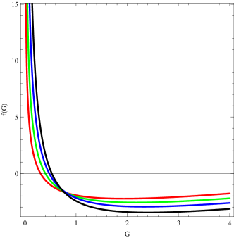
The first thing we want to do in this Section is to plot the NA $f(G)$ model (14) with respect to $G$ to check its behavior. For this purpose we assume four different values of $n$, i.e. $n=2.4,2.6,2.8,3$ and fix the other constants involved by taking the values as $c_{1}=0.5,c_{2}=3,c=0.5,~{}a_{0}=1$. Figure 1 shows the behavior of the model versus $G$. It represents the continuously decreasing manner of the function for $G<0.6$. The function approaches to the negative region and becomes approximately constant for $G>1$ incorporating all chosen values of $n$.

Figure 1: Plot of $f(G)$ versus $G$. The curves are characterize as red is for $n=2.4$, green is for $n=2.6$, blue is for $n=2.8$, black is for $n=3$.

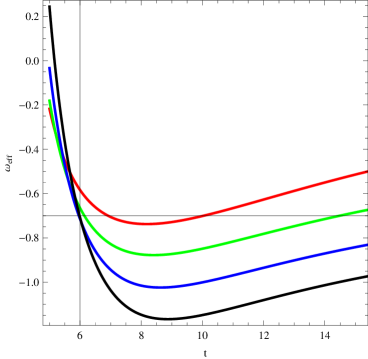
The EoS parameter $\omega_{eff}=\frac{p_{eff}}{\rho_{eff}}$ (using Eqs. (8) and (II) with corresponding quantities) is plotted against the cosmic time $t$ for same values of $n$ and constants as for Figure 1. Initially, the behavior of $\omega_{eff}$ indicates a decelerating phase of the universe as shown in Figure 2 as $\omega_{eff}<-\frac{1}{3}$ guarantees for the accelerated universe. Approximately for $5<t<6$, the graph enters into accelerated region referred as quintessence era, $-1<\omega_{eff}<-\frac{1}{3}$, for all values of $n$ considered. The universe remains in this region for $n=2.4$ and $2.6$ as shown by the EoS parameter. The higher values of $n$, i.e. $n=2.8$ and $3$, indicate the crossing of phantom divide line $\omega_{eff}=-1$ at $t=6.8$ and $7.6$ respectively and after this range, the universe faces the phantom era $\omega_{eff}<-1$. As time elapses, at $t=10$ and $14.5$, the universe again crosses the phantom divide line and becomes convergent in quintessence region. Thus, incorporating the first two values of $n$, the universe behaves as accelerated expanding in quintessence region and for last two values, the model depicts as quintom model (crossing of phantom divide line occurs).

Figure 2: Plot of $\omega_{eff}$ versus $t$. The curves are characterize as red is for $n=2.4$, green is for $n=2.6$, blue is for $n=2.8$, black is for $n=3$.

Figure 3: Plot of $v^{2}_{s}$ versus $t$. The curves are characterize as red is for $n=2.4$, green is for $n=2.6$, blue is for $n=2.8$, black is for $n=3$.

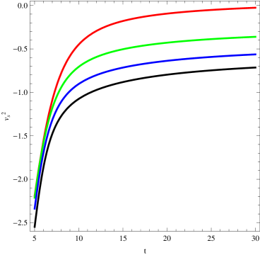
Figure 3 is a test to analyze the stability of the model by squared speed sound which defined as the ratio of the time derivative of total pressure to the time derivative of total energy density, i.e.:

$$v_{s}^{2}=\frac{\dot{p}_{eff}}{\dot{\rho}_{eff}}.$$ (15)

The stability or instability of the model depends upon the sign of this quantity. Its positive sign corresponds to a stable model while instability fits for negative values. The stability of many DE models is discussed using squared speed of sound. Setare setare3 studied the interacting HDE model with the generalized Chaplygin gas model and discussed that both models are instable. The agegraphic DE model is always negative which shows the instability of the model explored by Kim et al. kim . Jawad et al. jawad checked that the reconstructed HDE $f(G)$ model always remain instable.

Chattopadhyay and Pasqua Chattopadhyay reconstructed the HDE model in $f(T)$ gravity. They investigated that the squared speed of sound for reconstructed models bear negative values led to the classical instable models. Using Eqs.(8) and (II) for the NA $f(G)$ model, the $v^{2}_{s}$ versus time is plotted taking same values of $n$ and constants. The graph indicates the instability of the model for all values of $n$ as squared speed of sound remain negative during the its evolution. However, we may argue that for decreasing $n$ it gradually shifts towards zero $v^{2}_{s}$ and may cross it.

IV Statefinder parameters

Various candidates for the DE model have been proposed till date and we often face with the problem of discrimination between them. To get rid of this problem, Sahni et al. varun1 introduced the statefinder $\{r,s\}$ diagnostic pair. This pair has the following form varun1 ; varun2

$$r=\frac{\dddot{a}}{aH^{3}},\quad s=\frac{r-1}{3\left(q-\frac{1}{2}\right)}.$$ (16)

Here $q=-\frac{\ddot{a}}{aH^{2}}$ is the deceleration parameter and $H=\frac{\dot{a}}{a}$. Thus the diagnostic pair consists of the first, second and third derivatives of the scale factor and indicates geometrically the properties of DE. It has been discussed for a number of models. Sharif and Jawad sharif discussed the modified HDE in Kaluza-Klein universe and justified the limit of $\Lambda$CDM model by the statefinder pair. Panotopoulos Panotopoulos discussed this pair for two DE models. Chakraborty et al. Chakraborty discriminated different DE models in Kaluza-Klein universe. As demonstrated, the statefinder can successfully differentiate between a wide variety of DE models including the Chaplygin gas, the cosmological constant, braneworld models, quintessence and interacting DE models varun1 ; varun2 ; Zimdahl .

Figure 4: The $\{r-s\}$ trajectories. The red, green, blue and black lines correspond to $n=2.9,~{}2.8,~{}2.6$ and $2.4$ respectively. Other parameters are same as the previous figures.

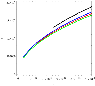
In the present work, based on the reconstructed energy density described in the previous Sections, we have created the $\{r-s\}$ trajectories. It is apparent from the $\{r-s\}$ trajectories created for different choices of parameters stated inside the caption of Figure 4 that the trajectories are confined inside the first quadrant of the $\{r-s\}$ plane. Moreover, it is observed that although the trajectories are tending towards the fixed point $\{r=1,s=0\}|_{\Lambda CDM}$, they can not reach it. Thus, it is inferred that the NA $f(G)$ model is not capable of reaching the $\Lambda$CDM phase of the universe.

V Conclusion

The search for best fit DE model is very challenging issue in cosmology recently. In this respect, the reconstruction phenomenon of different DE models gain a very eminent attention to discuss accelerated expansion of the universe. The correspondence of HDE, NADE, their entropy-corrected versions, ghost, scalar field models within modified gravities give consistent results. In this paper, we have taken the $f(G)$ gravity framework assuming exact power-law solution with dust matter. We have considered NADE model in this framework to explore the cosmic expansion of the universe. The NADE $f(G)$ model is reconstructed and we have used it for further prospective. The results are as summarized:

• The model contains highly nonlinear terms dependent upon $n$, thus we have drawn it for different $n$. The graphical behavior of NADE $f(G)$ model has shown the decreasing behavior against $G$.

• To characterize the different eras of the universe, we have plot EoS parameter versus time $t$ for different values of $n$. For smaller values, this parameter shows that the universe stays in the quintessence region. The higher values of $n$ represents the crossing of phantom divide line twice and the universe lying in quintessence state finally. Thus it is interesting to mention here that for $n=2.8$ and $3$, the reconstructed NA $f(G)$ model behaves like quintom model.

• The stability of the model is investigated by squared speed of sound. The NADE $f(G)$ model has preserved the instability during the evolution of the universe.

• The statefinder trajectories are plotted for the reconstructed model. It is observed that the NA $f(G)$ model is not subject to reach the $\Lambda$CDM model in the underlying scenario.

Jawad et al. jawad investigated the HDE model in the framework of $f(G)$ gravity to discuss the acceleration of the universe and checked the stability of the model with squared speed of sound. Also, they worked out on energy condition for HDE $f(G)$ model. In the present paper, we found the NADE $f(G)$ model by making correspondence between NADE model in the underlying gravity. The reconstructed HDE $f(G)$ model contains a linear term of $G$ and two nonlinear terms and shows the increasing behavior with respect to $G$. It shows the increasing behavior graphically. The reconstructed NADE $f(G)$ model inherits the same type of solution but highly nonlinear terms dependent upon $n$ with a constant term. Its graphical behavior represents the decreasing behavior. Both of the models remain instable during the evolution of the universe. However the violation of strong energy condition indicates the accelerated expansion for HDE $f(G)$ model whereas the quintessence region is observed for acceleration in NADE $f(G)$ gravity with the help of EoS parameter.

Acknowledgment

The first author (AJ) wishes to thank the Higher Education Commission, Islamabad, Pakistan for its financial support through the Indigenous Ph.D. 5000 Fellowship Program Batch-VII. The second author (SC) wishes to acknowledge the financial support from Department of Science and Technology, Govt. of India under Project Grant no. SR/FTP/PS-167/2011.

References

- (1) Cai, R.G.: Phys. Lett. B 657 (2007) 228.
- (2) Wei, H. and Cai, R.G.: Phys. Lett. B 660 (2008) 113.
- (3) Wei, H. and Cai, R.G.: Phys. Lett. B 663 (2008) 1.
- (4) Myung, Y.S. and Seo, M.G.: Phys. Lett. B 671 (2009) 435.
- (5) Nojiri, S. and Odintsov, S.D.: Phys. Lett. B 646 (2007) 105; ibid. B 659 (2008) 821.
- (6) Abdalla, M.C.B., Nojiri, S. and Odintsov, S.D.: Class. Quantum Grav. 22 (2005) L35.
- (7) Linder, E.V.: Phys. Rev. D 81 (2010) 127301.
- (8) Rastkar, A.R., Setare, M.R. and Darabi, F.: Astrophys. Space Sci. 337 (2012) 487.
- (9) Nojiri, S. and Odintsov, S.D.: Int. J. Geom. Meth. Mod. Phys. 4 (2007) 115.
- (10) Nojiri, S. and Odintsov, S.D.: Phys. Lett. B 631 (2005) 1.
- (11) Davis, S.C.: arXiv:0709.4453.
- (12) Setare, M.R. and Saridakis, E.N.: Phys. Lett. B 670 (2008) 1.
- (13) Liu, X.L. and Zhang, X.: Commun. Theor. Phys. 52 (2009) 761.
- (14) Setare, M.R.: Astrophys. Space Sci. 326 (2010) 27.
- (15) Jamil, M. and Saridakis, E.N.: JCAP 1007 (2010) 028.
- (16) Setare, M.R. and Jamil, M.: Europhys. Lett. 92 (2010) 49003.
- (17) Jawad, A., Pasqua, A. and Chattopadhyay, S.: Astrophys. Space Sci. (2013, to appear).
- (18) Setare, M.R.: Phys. Lett. B 654 (2007) 1.
- (19) Kim, K.Y., Lee, H.W. and Myung, Y.S.: Phys. Lett. B 660 (2008) 118.
- (20) Chattopadhyay, S. and Pasqua, A.: Astrophys. Space Sci. (2013, to appear).
- (21) Sahni, V., Saini, T.D., Starobinsky, A.A. and Alam, U.: JETP Lett. 77 (2003) 201.
- (22) Sahni, V., Shafieloo, A. and Starobinsky, A.A.: Phys. Rev. D 78 (2008) 103502.
- (23) Sharif, M. and Jawad, A.: Europ. Phys. J. C 72 (2012) 1901.
- (24) Panotopoulos, G.: Nuc. Phys. B 796 (2008) 66.
- (25) Chakraborty, S., Debnath, U., Jamil, M. and Myrzakulov, R.: Int. J. Theor. Phys. 51 (2012) 2246.
- (26) Zimdahl, W. and Pavon, D.: Gen. Rel. Grav. 36 (2004) 1483.