Galaxy and Mass Assembly (GAMA): The halo mass of galaxy groups from maximum-likelihood weak lensing

Abstract

We present a maximum-likelihood weak lensing analysis of the mass distribution in optically selected spectroscopic Galaxy Groups (G³Cv5) in the Galaxy And Mass Assembly (GAMA) survey, using background Sloan Digital Sky Survey (SDSS) photometric galaxies. The scaling of halo mass, $M_{h}$, with various group observables is investigated. Our main results are: 1) the measured relations of halo mass with group luminosity, virial volume and central galaxy stellar mass, $M_{\star}$, agree very well with predictions from mock group catalogues constructed from a GALFORM semi-analytical galaxy formation model implemented in the Millennium $\Lambda$CDM N-body simulation; 2) the measured relations of halo mass with velocity dispersion and projected half-abundance radius show weak tension with mock predictions, hinting at problems in the mock galaxy dynamics and their small scale distribution; 3) the median $M_{h}|M_{\star}$ measured from weak lensing depends more sensitively on the lognormal dispersion in $M_{\star}$ at fixed $M_{h}$ than it does on the median $M_{\star}|M_{h}$. Our measurements suggest an intrinsic dispersion of $\sigma_{\log(M_{\star})}\sim 0.15$; 4) Comparing our mass estimates with those in the catalogue, we find that the G³Cv5 mass can give biased results when used to select subsets of the group sample. Of the various new halo mass estimators that we calibrate using our weak lensing measurements, group luminosity is the best single-proxy estimator of group mass.

1 Introduction

Even though the nature of dark matter will ultimately be determined by observations of its particle properties, its gravitational effect has so far been the cleanest way to map its distribution in the universe. Weak gravitational lensing is one of the main techniques for mapping dark matter on large and intermediate scales (e.g. Bartelmann & Schneider, 2001). As its name suggests, weak lensing is the production of weak distortions (shear) in the shapes of background, or source, galaxies by foreground masses. Usually one has no prior knowledge of the intrinsic shape of a source galaxy, resulting in uncertainties much larger than the gravitational shear signal, so the extraction of shape distortions has to be done in a statistical way, for example by measuring the shear-shear correlation function on large scales (e.g., Kilbinger et al., 2013), or by stacking a large number of source galaxies around many lenses on smaller scales. Early applications of stacked lensing to low mass groups have been carried out by Hoekstra et al. (2001) and Parker et al. (2005) who measured the average mass-to-light ratio of groups in the Canadian Network for Observational Cosmology Field Galaxy Redshift Survey (CNOC2). Stacked lensing measurements have also been made using galaxies and groups in many current large surveys, including the SDSS (Mandelbaum et al., 2006a, b; Johnston et al., 2007; Sheldon et al., 2009), CFHT Lensing Survey (Velander et al., 2013; Hudson et al., 2013), COSMOS (Leauthaud et al., 2012) and Deep Lens Survey (Choi et al., 2012). These studies estimate the average density profile of the dark matter haloes of the lenses, and derive scaling relations between halo mass and other observational properties.

Even though stacked lensing analyses can give a non-parametric estimate of the matter density profile around lenses with similar properties, the interpretation of the stacked signal can be difficult. This is because the stacked profile is an average over all the contributing haloes of unknown mass distribution, and this average typically has a complicated weighting determined by the error of each shape measurement, the number of pairs within each radial bin, and the redshifts of lenses and sources. To account somewhat for these averaging effects, one usually parametrizes the distribution of halo masses and the clustering of haloes using the framework of halo occupation distribution (HOD) models (e.g. Cooray & Sheth, 2002; Mandelbaum et al., 2005b; Leauthaud et al., 2012), and fits for the HOD parameters given the stacked profiles.

In this work we carry out a weak lensing analysis of galaxy groups from the Galaxy And Mass Assembly (GAMA, Driver et al., 2011) survey. GAMA is an ongoing spectroscopic survey of moderate sky coverage. As large scale surveys go, it has deep spectroscopy as well as uniform, yet high, completeness ($>98$%) down to $r_{\rm AB}=19.8$. This makes possible the construction of a large and accurate galaxy group catalogue (G³Cv5, Robotham et al., 2011), able to reach lower halo masses than other existing catalogues of the local universe. In addition, the survey region of GAMA was selected to overlap several companion surveys at different wavelengths, ranging from radio to x-ray. These complementary data provide a detailed picture of the properties of GAMA galaxies. The variation of galaxy properties with environment, defined by the mass distribution probed by weak lensing, can be investigated using gravitational shear measurements of background galaxies taken from the photometric SDSS data in the same region. Fortunately, the redshift distribution of GAMA groups peaks at $z\sim 0.2$, where the lensing efficiency of the SDSS galaxy sample also peaks. These lens and source samples are described in more detail in Section 2. Since our default lens sample is subject to a survey flux limit and a group multiplicity selection, most of the measured mass-observable relations in this work are subject to some selection effects and should not be taken as general relations for a volume-limited sample. In order to draw some general conclusions on galaxy formation, however, we only compare our measurements with mock galaxy catalogues that incorporate the same selection function. These mock catalogues are also described in Section 2.

As the galaxy number density of our source sample ($\sim 1~{}\mathrm{arcmin}^{-2}$) is much lower than some dedicated lensing surveys (e.g., $\sim 20~{}\mathrm{arcmin}^{-2}$ in CFHTLS and $\sim 70~{}\mathrm{arcmin}^{-2}$ in COSMOS), and because the lens sample is restricted by the small GAMA sky coverage ($\sim 150\mathrm{deg}^{2}$ in this work) compared with SDSS for instance, we do not have any obvious advantage in signal-to-noise over existing measurements. Hence efficient utilization of the lensing signal is crucial to our analysis. To this end, we go beyond the popular stacked analyses, and perform a maximum-likelihood analysis on the shapes of individual background galaxies, broadly following the method in Hudson et al. (1998) (see also Schneider & Rix, 1997; Hoekstra et al., 2003, 2004). The key difference between our approach and stacked lensing is that we fit the shapes of each source galaxy explicitly, while stacked lensing only estimates or fits the average tangential shear for sub-samples of sources binned in radius, and around lenses binned according to mass proxies. Our method requires no binning in the source sample, and can be applied with or without binning in the lens sample. Not binning the data avoids information losses, leading to good measurements with our small sample. Another advantage of our method is that it is free from the averaging ambiguity associated with stacking, since the mass of each lens is explicitly modelled. With this method, the large number of available observational properties associated with GAMA groups can now all be linked with the underlying halo masses, to provide valuable constraints on galaxy formation models. We will also show that our maximum-likelihood weak lensing method is an ideal tool for model selection, to pick up the tightest mass-observable relation observationally. We describe our method in Section 3, and its practical application in Section 4.

As a first application of our maximum-likelihood weak lensing (MLWL) method, we extract the scaling relations of halo mass to various group observables, including velocity dispersion, luminosity, radius, virial volume and stellar mass of the group’s central galaxy. With MLWL we give both non-parametric measurements of these relations by binning only the lens sample according to observable, and parametric fits by modelling the mass-observable relation as a power-law with no binning at all. The G³Cv5 comes with estimated halo masses calibrated using mock catalogues. These mass estimates are also examined with MLWL, to see if they differ from our measurements. Starting from MLWL we also construct several new mass estimators, which we compare with predictions from a semi-analytical galaxy formation model and previous measurements. These results are described and discussed in Sections 5 and 6, with all the fits summarized in Table 1.

Weak lensing measurements can be compared with predictions from galaxy formation models to gain insight into the various physical processes in the model. In this comparison, it is crucial that one properly accounts for the observational selection effects. Hilbert & White (2010) first compared the weak lensing measured mass-richness relation with the prediction from semi-analytic galaxy formation models. They construct mock clusters by picking cluster haloes from simulation snapshots, and applying observational selection functions to the member galaxies of the mock clusters. In this work, we improve the treatment of selection effects in two aspects. First, a light-cone galaxy catalogue (Merson et al., 2013) is constructed from a semi-analytic galaxy formation model, to account fully for the selection function of the galaxy survey. Second, identical group finding algorithms (Robotham et al., 2011) are applied to both the real and mock galaxy catalogues, to account fully for the selection effect introduced by group finding. We also have compared many more mass-observable relations. All the relations in Table 1 are subject to sample selection, and we only compare them with mock catalogues constructed with the same selection function as the real data. The only exception is in the comparison of our stellar mass-halo mass relation with those from other works, where we make an additional measurement for a volume-limited central galaxy sample.

To summarize the structure of the paper, we describe our lens and source samples in Section 2 along with the mock catalogues to which we compare our measurements; the general MLWL method is described in Section 3, with its application to our samples described in Section 4; the results are presented and discussed in Sections 5 and 6; finally, we conclude in Section 7.

The units throughout this paper, wherever not explicitly specified, are ${\rm km\,s}^{-1}$ for velocity, $h^{-1}\rm{Mpc}$ for length, $h^{-1}\mathrm{M}_{\odot}$ for halo mass, $h^{-2}\mathrm{M}_{\odot}$ for galaxy stellar mass, and $h^{-2}\mathrm{L}_{\odot}$ for luminosity, where $H_{0}=100h$ km s^-1 Mpc^-1. The $\log()$ function throughout is the common (base 10) logarithm, while the natural logarithm is $\ln()$. Unless explicitly stated, the lens sample covers groups with three or more members. The relevant cosmological parameters, which only appear in the distance calculations of our measurements, are $\Omega_{M}=0.3$ and $\Omega_{\Lambda}=0.7$.

2 Data Samples

The lens and source samples used in this work are described in detail in Sections 2.1 and 2.2 respectively. Section 2.3 contains a description of the mock GAMA group catalogues, to which we compare our measurements.

2.1 Lens Catalogue: GAMA Galaxy Group Catalogue (G³Cv5)

We use the fifth version of the GAMA Galaxy Group Catalogue (Robotham et al., 2011, hereafter G³Cv5) in the three equatorial GAMA regions ($12\times 4~{}\rm{deg}^{2}$ each) as our lens sample. The galaxy groups were identified in the 3-year GAMA I data using a modified Friends-of-Friends (FoF) algorithm (Eke et al., 2004a) and calibrated against a set of mock catalogues constructed from the GALFORM (Bower et al., 2006) semi-analytical model, following the method described in Merson et al. (2013). The GAMA I data used here are uniformly limited to $r_{\rm AB}=19.4$ across the three regions. Group properties are found to be robust to the effects of interlopers and are median unbiased. The G³Cv5 catalogue contains $\sim 12200$ groups with two or more members and includes $\sim 50\%$ of all the GAMA galaxies down to a magnitude limit of $r_{\rm AB}\leq 19.4$.

Applying the G³Cv5 group finding algorithm to mock GAMA surveys shows that approximately half of the two-member groups contain galaxies from different dark matter haloes. These groups would have particularly unreliable properties, so we exclude all binary groups from this study, reducing the sample to $\sim 4500$ groups. In addition, we exclude groups for which the measured velocity dispersion is smaller than the assumed velocity measurement errors or for which the stellar mass of the central galaxy has not been estimated (mainly due to missing photometry in the GAMA I reprocessed multi-wavelength imaging; Hill et al., 2011; Kelvin et al., 2012; Taylor et al., 2011). This removes a further 164 groups. The central galaxy of the group is defined in the iterative way recommended by Robotham et al. (2011), where the galaxy furthest from the galaxy luminosity-weighted projected centre is rejected and this process repeated until the brighter of the final two galaxies is chosen. This is the preferred choice of centre according to Robotham et al. (2011) who find the iterative centre to be less affected by interlopers than the Brightest Cluster Galaxy (BCG) or the luminosity-weighted centre. We use these iterative central galaxies to define the centres of our groups. This central galaxy is identical to the BCG for $\sim 90$% of the groups, and it makes little difference in our measurement if we choose the BCG as group centre instead. Stellar masses for group central galaxies were inferred using a stellar population synthesis model, adopting a Chabrier IMF (Taylor et al., 2011).

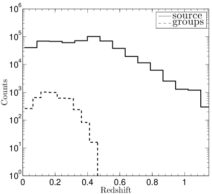
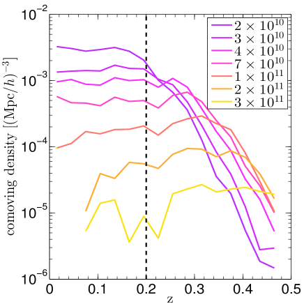
The redshift distribution of our group sample, i.e. lens catalogue, is shown in the lower panel of Fig. 1, peaking at $z\sim 0.2$ and extending to $z\sim 0.5$.

2.1.1 $\mathrm{G}^{3}\mathrm{Cv5}$ Mass Estimators

For each GAMA group, after measuring the group velocity dispersion with the gapper estimator (Beers et al., 1990) and correcting for a velocity measurement error, the dynamical mass of the group is estimated via

$$M_{\rm dyn}\,=\,A_{\rm dyn}\,\sigma_{v}^{2}\,R_{50}.$$ (1)

$R_{50}$ is the projected half-abundance radius containing 50 percent of the group members (Robotham et al., 2011). We adopt this definition of group radius throughout this paper. The prefactor $A_{\rm dyn}\sim 10$ was calibrated as a function of redshift and multiplicity in the mock catalogues by Robotham et al. (2011). The mass definition used in the calibration process is not exactly the commonly used $M_{200b}$, but closely related to it as mentioned in Robotham et al. (2011)(see Jiang et al., 2013, for more details of the exact mass definition used and how it compares to $M_{200b}$). The other G³Cv5 mass estimator, the luminosity mass, comes from rescaling the total group luminosity

$$M_{\rm lum}\,=\,A_{\rm lum}\,L_{\rm grp}.$$ (2)

$L_{\rm grp}$ is the total $r$-band luminosity of the group, corrected for the fraction of light in galaxies below the survey flux limit using the GAMA luminosity function (Robotham et al., 2011). Throughout this paper we refer to the $r$-band $L_{\rm grp}$ as the group luminosity. Most of the GAMA groups contain members fainter than $M^{*}=-20.44+5\log h$ (Blanton et al., 2003; Loveday et al., 2012), and the group luminosity is dominated by galaxies around $M^{*}$, so the correction factor is below $3$ for about $90$ per cent of the groups and $\sim 2$ at $z=0.2$, the median group redshift. The prefactor $A_{\rm lum}$ is calibrated using $M_{\rm dyn}$ for the observed groups as a function of redshift and multiplicity. Consequently, $M_{\rm lum}$ is median unbiased with respect to $M_{\rm dyn}$.

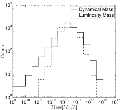
As shown in the top panel of Fig. 1, the GAMA groups mainly reside in haloes of $10^{13}-10^{14}h^{-1}\mathrm{M}_{\odot}$. The dynamical mass has a broader distribution than the luminosity mass, reflecting the larger dispersion in the former estimate, particularly for the groups with low membership. We find that the same luminosity mass calibration method applied to the mock groups suggests that halo mass should be more tightly correlated with luminosity mass than with dynamical mass.

Figure 1: The mass and redshift distributions of our lens and source samples. Upper panel: distribution of the G³Cv5 dynamical and luminosity mass estimates for our group sample. Lower panel: redshift distribution of our GAMA group sample and the SDSS source galaxies. Note that only groups with at least three members are considered in this work.

2.2 Source Catalogue: SDSS shape measurements

We use as source galaxies those from the SDSS DR7 within and around the three GAMA regions. The approach we follow is to measure a per-galaxy shape distortion, and then relate those to the shear applied to the ensemble of galaxies. The shapes of these galaxies are measured by Mandelbaum et al. (2005a) and Reyes et al. (2012) using the re-Gaussianisation technique, which we briefly describe in Appendix A for completeness. As recommended by Mandelbaum et al. (2005a) and Reyes et al. (2012), we keep only those galaxies with extinction-corrected $r$-band model magnitudes brighter than 21.8, $r$-band extinction below 0.2, and galaxy resolution above $1/3$ in both the $r$ and $i$ bands. The photometric redshifts of these galaxies are estimated using the template fitting algorithm ZEBRA (Feldmann et al., 2006), the application of which in weak lensing is thoroughly discussed by Nakajima et al. (2012). We further require that the ZEBRA photo-$z$ determinations are successful using a non-starburst template, considering the typically large photo-$z$ errors for starburst galaxies. The final sample consists of $\sim 5.6\times 10^{5}$ galaxies, corresponding to a number density of $\sim 1~{}\rm{arcmin}^{-2}$. The lower panel of Fig. 1 shows the distribution of galaxy photo-$z$ values, which peaks around $z=0.5$ and extends to $z>1.0$. The use of photo-$z$s for source galaxies could introduce a bias and boost the error in our lensing mass measurement. We address these issues with the help of Monte-Carlo simulations as detailed in Section 3.5, 4.2 and 5.1.

2.2.1 Galaxy ellipticity

For a purely elliptical galaxy image following a 2D Gaussian brightness profile, its shape can be simply quantified by the axis ratio and the direction of the major axis. Equivalently, we can measure an ellipticity, $\boldsymbol{\chi}=(\chi_{1},\chi_{2})$, defined as

$$\chi_{1}+i\chi_{2}=\frac{1-q^{2}}{1+q^{2}}e^{i2\phi},$$ (3)

where $q$ is the minor to major axis ratio. $\phi$ is the position angle of the major axis, defined in a reference frame where the positive $x$ and $y$ axes point to the east and the north on the sky respectively. Note that the ellipticity is not a vector, since a rotation of the reference frame by $\psi$ transforms $\boldsymbol{\chi}$ as

$$\left(\begin{array}[]{c}\chi_{1}^{\prime}\\ \chi_{2}^{\prime}\end{array}\right)=R(-2\psi)\left(\begin{array}[]{c}\chi_{1}\\ \chi_{2}\end{array}\right)$$ (4)

, where

$$R(\theta)=\begin{pmatrix}\cos\theta&\sin\theta\\ -\sin\theta&\cos\theta\end{pmatrix}$$ (5)

is the rotation matrix. However, we still write it in a vector form to simplify equations involving dot products of ellipticities and shears later, where $\boldsymbol{\chi}\cdot\boldsymbol{\chi}^{\prime}=\chi_{1}\chi_{1}^{\prime}+\chi_{2}\chi_{2}^{\prime}$.

A real galaxy image is typically the convolution of a non-Gaussian intrinsic image with a non-Gaussian point spread function (PSF). In Appendix A, we describe how we measure the ellipticities for real galaxies. How the ellipticity relates to the lens distribution will be described in Section 3.1.

2.3 Mock Group Catalogues: Millennium light-cones

The GAMA group finder has been run on a set of nine light-cone mock galaxy catalogues by Robotham et al. (2011) to produce mock group catalogues that allow us to compare the model predictions with observations and investigate sample variance. The mock galaxy catalogues were created following the approach developed by Merson et al. (2013), briefly summarised here.

Firstly a GALFORM semi-analytical galaxy formation model (Bower et al., 2006, in this case) is run on merger trees extracted from the Millennium simulation (Springel et al., 2005) to create the galaxy distribution within each simulation snapshot. Using the individual snapshots (with replications if necessary), a galaxy lightcone is generated by sampling the galaxies according to their redshift and distance away from the observer. An interpolation on galaxy position, velocity and k-correction is applied between snapshots to avoid any abrupt transitions or features at snaphot boundaries. All other galaxy properties are fixed to the earlier snapshot. Finally the GAMA survey selection function is applied to the galaxies in the lightcone to produce a mock GAMA survey. When applying the survey selection function we force the mock luminosity function to reproduce perfectly the observed luminosity function, by abundance matching. This changes the $r$-band magnitudes of the original GALFORM predicted magnitudes by less than 0.15 mags typically.

This process is repeated for each of the nine different GAMA lightcone mocks, all extracted from the same Millennium simulation, with some limited attempt at reducing any overlap between each of them. Futher details of their construction and limitations are given in Robotham et al. (2011) and Merson et al. (2013).

The G³Cv5 grouping algorithm was run on these GAMA mock surveys, yielding the so-called mock group catalogues. Each mock group has the same set of observational properties (and measured in exactly the same way) as the real GAMA groups. For the purpose of this study, we also associate a true halo mass, $M_{h}$, with each group by selecting the mass of the dark matter halo hosting the iteratively-determined central galaxy of the mock group.

3 Method: Maximum Likelihood Weak Lensing

One might wonder whether the Maximum Likelihood Weak Lensing (MLWL) technique is simply stacked weak lensing extended to the unbinned limit, that is, the case in which one has at most a single lens-source pair inside each bin. While stacked weak lensing usually works pair by pair for all the lens-source pairs, the MLWL method used here operates source by source. With $N_{s}$ source galaxies one has $2N_{s}$ independent observables since each source galaxy has two ellipticity components (see Equation (3)). Coupled with $N_{\ell}$ lens galaxies, this gives $N_{\ell}N_{s}$ tangential shear measurements. However, these $N_{\ell}N_{s}$ pairs are generally not independent, and the covariance matrix of these measurements has at most $2N_{s}$ non-zero eigenvalues. Hence the matrix is not invertible when $N_{\ell}N_{s}>2N_{s}$ and, in this case, it is not possible to write down the joint probability distribution function (PDF) of these variables. In other words, attempts to extend stacked lensing to the unbinned limit will fail when the total number of radial bins from all the mass bins exceeds the intrinsic number of degrees of freedom in the source sample ($2N_{s}$). However, there is still a PDF associated with the dataset in the unbinned case when one works in the eigenspace, i.e. directly with the shear of each source galaxy rather than the tangential shear of each lens-source pair, as we do here.

We start by describing the ellipticity of each source galaxy with a 2 dimensional Gaussian distribution, which enables us to write down a likelihood function combining all the source galaxies. The model dependence enters through the expected ellipticity of each source. This is achieved by modelling the predicted ellipticity field as a superposition of the shear field from all the foreground lenses. Each lens is modelled as a circularly symmetric mass distribution with a single parameter. In principle, the mass parameter of all the lens haloes can be estimated simultaneously by optimizing the joint likelihood of all the source ellipticities. However, this means a parameter space with a dimensionality of the number of lenses, $\sim 4500$ for our sample, which is not easily manageable. Besides, the huge number of parameters also means extremely low signal to noise for the estimate of each individual parameter. Instead of fitting the mass of each halo explicitly, we reduce the dimensionality by predicting their masses from group observables (e.g., group luminosity), and only fit the parameters of a mass-observable relation. We also take a second approach by dividing the sample into a small number of bins according to observables, and fit a single mass to all the haloes within each bin. In the following subsections we give a detailed description of our implementation.

3.1 Predicting the ellipticity of source galaxies

The shear field, generated by foreground lenses, transforms the intrinsic ellipticities of source galaxies into observed ellipticities. To linear order, with our definition the ellipticity transforms under a small applied shear $|\boldsymbol{\gamma}|\ll 1$ as (e.g., Bernstein & Jarvis, 2002)

$$\boldsymbol{\chi}=\boldsymbol{\chi}_{0}+2\boldsymbol{\gamma}-(2\boldsymbol{\gamma}\cdot\boldsymbol{\chi}_{0})\boldsymbol{\chi}_{0}.$$ (6)

If the intrinsic ellipticity, $\boldsymbol{\chi}_{0}$, of each galaxy is randomly oriented with no correlation between its two components, then the expectation value of the observed ellipticity can be found from Equation (6) as

$$\mathrm{E}[\boldsymbol{\chi}]=2\mathscr{R}\boldsymbol{\gamma},$$ (7)

with

$$\mathscr{R}=1-\sigma_{SN}^{2}$$ (8)

being the shear responsivity (Bernstein & Jarvis, 2002). Here $\sigma_{SN}^{2}=\mathrm{E}[\chi_{0,1}^{2}]=\mathrm{E}[\chi_{0,2}^{2}]$ is the intrinsic shape noise. In the presence of measurement errors, the responsivity (Equation 8) is still valid, and can be equivalently derived from the more general Equation (5.33) in Bernstein & Jarvis (2002) with a constant weight function.

It also follows from Equation (6) that when $|\boldsymbol{\gamma}|\ll 1$, the predicted ellipticity $\hat{\boldsymbol{\chi}}={\rm E}[\boldsymbol{\chi}]$ due to the shear contribution from different lenses adds up linearly for the same source:

$$\left(\begin{array}[]{c}\hat{\chi}_{1}\\ \hat{\chi_{2}}\end{array}\right)=2\mathscr{R}\sum_{\ell}R(2\phi_{\ell}+\pi)\left(\begin{array}[]{c}\gamma_{t,\ell}\\ \gamma_{\times,\ell}\end{array}\right)$$ (13)

where $R(\theta)$ is the rotation matrix defined in Equation (5), $\gamma_{t,\ell}$ and $\gamma_{\times,\ell}$ are the tangential and cross shear produced by lens $\ell$ at the position of the source, and $\phi_{\ell}$ is the position angle of the lens in the reference frame of the source. Note the tangential reference frame is rotated by $\phi_{\ell}+\pi/2$ from the local source frame. The summation runs over all contributing lenses (i.e., foreground haloes).

3.2 Lens models

We model the mass distribution of each group as a spherical NFW (Navarro et al., 1996, 1997) halo, with a single parameter, $M$, defined as the virial mass such that the average matter density inside the virial radius equals 200 times the mean density of the universe. The concentration parameter is fixed as in Duffy et al. (2008),

$$c=10.14\left(\frac{M}{2\times 10^{12}h^{-1}\mathrm{M}_{\odot}}\right)^{-0.081}(1+z)^{-1.01}.$$ (14)

The data used in this study are consistent with these assumptions, but do not provide sufficient leverage to fit the internal halo profile while also determining the dependence of total mass on other group observables; hence the restricted lens model adopted here. We denote the virial radius following this definition as $R_{200b}$. We also considered a central point source component representing the stellar mass of the central galaxy, but found it had almost no impact on the results and can be safely ignored for this analysis. In this work we have also neglected the contribution to the lensing signal from line-of-sight structures, the impact of lens group asymmetries, and contamination from radial alignments of group member galaxies. Previous studies (Marian et al., 2010; Schneider et al., 2012, 2013) suggest that these effects are likely to be present at a level of no more than a few per cent. The contributions from these uncertainties, as well as the contributions from any lenses absent from our sample to the observed source shapes, are effectively considered as part of the intrinsic shape noise.

These circularly symmetric lenses induce only tangential shear in the source images,

$$\gamma_{\times,\ell} =0\mbox{~{}~{}and}$$ (15)

$$\gamma_{t,\ell} =\frac{\Delta\Sigma}{\Sigma_{\rm crit}}$$ (16)

(see e.g. Schneider, 2005). Here $\Delta\Sigma=\Sigma(<r)-\Sigma(r)$ is the difference between the mean physical surface overdensity, $\Sigma$, within a radius $r$ and that at $r$. Analytical expressions for $\Delta\Sigma(r)$ for NFW haloes can be found in Wright & Brainerd (2000). The critical physical surface density is defined as

$$\Sigma_{\rm crit}=\frac{c^{2}}{4\pi G}\frac{D_{s}}{D_{\ell s}D_{\ell}},$$ (17)

where $D_{\ell}$, $D_{s}$ and $D_{\ell s}$ are the angular diameter distances to the lens, the source and that between the two respectively. In calculating these distances we adopt the fitting formula of Adachi & Kasai (2012), which is accurate to within 1 percent, for relevant cosmologies.

3.3 Likelihood function

Following Hudson et al. (1998), we assume the noise in the observed $\boldsymbol{\chi}$ follows a bi-variate Gaussian distribution. The probability of observing each source galaxy with shape $\boldsymbol{\chi}=(\chi_{1},\chi_{2})$ is given as:

$$p(\boldsymbol{\chi}|\hat{\boldsymbol{\chi}})=\frac{1}{2\pi\sigma^{2}}e^{-\left[\frac{(\chi_{1}-\hat{\chi}_{1})^{2}}{2\sigma^{2}}+\frac{(\chi_{2}-\hat{\chi}_{2})^{2}}{2\sigma^{2}}\right]},$$ (18)

where the single-component variance, $\sigma^{2}=\sigma_{\chi}^{2}+\sigma_{SN}^{2}$, is the sum of the measurement noise, $\sigma_{\chi}$, and intrinsic shape noise, $\sigma_{SN}$. For our source sample, $\sigma_{SN}\simeq 0.4$ (Mandelbaum et al., 2005a) provides the dominant contribution to the total noise.  The predicted ellipticity, $\hat{\boldsymbol{\chi}}$, is given by Equations (13), (15) and (16).

The likelihood function of our full lens-source sample is written as,

$$L=\prod_{i}p_{i},$$ (19)

where $i$ runs over all the source galaxies. In principle, an imperfect PSF correction could break the statistical independence of the likelihoods for individual source galaxies so the combined likelihood is no longer a simple product as above. Even in this case, however, the large shape noise will make Equation (19) true to good approximation.

3.4 Likelihood ratio

The log-likelihood function can be written as

$$\ln(L/L_{0})=\sum_{i}\left[\frac{(2\boldsymbol{\chi}-\hat{\boldsymbol{\chi}})\cdot\hat{\boldsymbol{\chi}}}{2\sigma^{2}}\right]_{i},$$ (20)

where $\ln L_{0}$ is a constant quantifying the log-likelihood of the observed shapes given a model that predicts no gravitational shear. This $L_{0}$ is independent of the model parameters, varying only with the data.

The observed ellipticity is the sum of a true ellipticity, produced by the gravitational shear from the entire mass distribution, and a noise component, i.e. $\boldsymbol{\chi}=\boldsymbol{\chi}_{T}+\boldsymbol{\epsilon}$, while the predicted ellipticity can be written in terms of a difference from the true shear-induced ellipticity, through $\hat{\boldsymbol{\chi}}=\boldsymbol{\chi}_{T}-\boldsymbol{\chi}_{\Delta}$. Note $\boldsymbol{\chi}_{\Delta}=0$ would correspond to a perfect model. With this decomposition, the likelihood ratio reduces to

$$2\ln(L/L_{0}) =\sum_{i}\left(\frac{\boldsymbol{\chi}_{T}^{2}-\boldsymbol{\chi}_{\Delta}^{2}+2\boldsymbol{\epsilon}\cdot\hat{\boldsymbol{\chi}}}{\sigma^{2}}\right)_{i}$$ (21)

$$=\sum_{i}\left(\frac{S}{N}\right)_{i}^{2}-\left(\frac{\Delta S}{N}\right)_{i}^{2}+\left(\frac{2C_{MN}}{N^{2}}\right)_{i},$$ (22)

with the first term representing the signal-to-noise ratio of the data, the second term deriving from discrepancies between the model and actual gravitational shears, and the last term being the model-noise cross-correlation.

Intrinsic alignments of background galaxies and systematic biases in the measured ellipticities can both produce regions of the survey in which $\langle\boldsymbol{\epsilon}\rangle\neq 0$. In addition, the predicted ellipticities near to survey boundaries will typically have a preferential alignment, because no contribution is taken into account in the model from lenses just outside the survey region. Consequently, the model-noise cross-correlation term in equation (22) may well be non-zero near to the edges of the survey region, meaning that the most likely model will be biased by this cross-correlation. In stacked weak lensing, this cross-correlation term shows up as systematic shear (see e.g. Hirata et al., 2004; Mandelbaum et al., 2005a). It can equivalently be understood as the non-zero residual of tangential shear averaged inside boundary-crossing annuli around sources. This systematic shear can be avoided by excluding the contribution to the source galaxy predicted ellipticity from any lens more distant than the nearest survey boundary, as we will do in Section 4.1.

In the absence of the cross-correlation term, the interpretation of the likelihood ratio is now clear: it is simply the difference between the signal-to-noise ratio in the data and that from the model deficiency. Since $L_{0}$ is model independent, maximizing the likelihood function is equivalent to minimizing the model deficiency. This makes MLWL an ideal tool to search for the tightest mass-observable relations, or the least-scatter halo mass estimators, as we will do in Section 6.2.

According to Equation (22), one needs to avoid regions in the dataset where $|\Delta S|\gtrsim S$ is expected, to avoid degrading the overall signal-to-noise or producing biased fits. It also becomes clear from Equation (22) that stacking or binning reduces the signal-to-noise by averaging the model within each bin, thus contributing to the model deficiency term.

More generally, one can define a test statistic

$$TS=2\ln(L/L_{0}),$$ (23)

where $L$ is the maximum likelihood value of a full model while $L_{0}$ is that of the same model with some parameters fixed (the null model). According to Wilks’s theorem (Wilks, 1938), if the data follow from the null model, then $TS$ follows a $\chi^{2}$ distribution with $n$ degrees of freedom, where $n$ is the difference between the number of free parameters in the full and null models. For a measured $TS$, the probability that such a large $TS$ is compatible with noise, or the $p$-value, is simply $p=P(\chi^{2}_{n}>TS)$. This can be converted to a Gaussian significance of $\Phi^{-1}(1-p/2)~{}\sigma$, where the function $\Phi^{-1}$ is the quantile function of the Gaussian distribution. The covariance among parameters can also be estimated from the Hessian matrix of the likelihood ratio with respect to the parameters. Expanding the likelihood ratio locally around the maximum-likelihood value to leading order, we have

$$\delta TS=\delta{\bf c}^{T}H\delta{\bf c},$$ (24)

where $\mathbf{c}$ is a column vector of model parameters, and $H=\nabla_{c}\ln(L)$ is the Hessian matrix. $\delta TS$ is now the likelihood ratio with respect to a null model at $\mathbf{c}+\delta\mathbf{c}$. Setting $\delta TS=1$, the $p=0.317$ critical value of the $\chi^{2}$ distribution, one obtains the covariance matrix of parameters as ${\Sigma}_{\rm cov}={H}^{-1}$. Alternatively, the errors on the parameters can be estimated using random catalogues, which are particularly useful when accounting for additional systematics. This will be described in Sections 3.5 and 4.2.

3.5 Prior distribution of nuisance parameters

So far we have assumed that the only uncertainties come from the measured shapes of the source galaxies. However, the likelihood function depends implicitly on the redshift of each source galaxy and the inferred centre and predicted mass for each lens. The uncertainties in these implicit parameters can be accounted for by marginalizing over their prior distributions. With any observed source redshift, $z_{o}$, observed lens centre, $\mathbf{X}_{o}$, and predicted lens mass, $M_{o}$, the probability distributions of the actual values can be written as $P(z|z_{o})$, $P(\mathbf{X}|\mathbf{X}_{o})$ and $P(M|M_{o})$. Given knowledge about these additional stochastic processes, the likelihood function can be more generally written as

$$L=\int \prod_{s=1}^{m}p(\boldsymbol{\chi}_{s}|z_{s},\mathbf{X}_{1},\mathbf{X}_{2},...\mathbf{X}_{n},M_{1},M_{2},...M_{n})$$ (25)

$$dP(z_{s}|z_{o,s})\prod_{\ell=1}^{n}dP(\mathbf{X}_{\ell}|\mathbf{X}_{o,\ell})dP(M_{\ell}|M_{o,\ell}),$$

where the subscripts $s$ and $\ell$ represent different sources and lenses in the sample. The above equation arises from assuming independent prior distributions, $P(z_{s}|z_{o,s})$, $P(\mathbf{X}_{\ell}|\mathbf{X}_{o,\ell})$ and $P(M_{\ell}|M_{o,\ell})$, for the different sources and lenses, although it is straightforward to generalise to correlated distributions.

Equation (25) is too computationally intensive to solve directly. Instead, we take an indirect approach in our likelihood optimization and continue to use Equation (19) as our likelihood function. Ignoring the stochastic processes mentioned above should lead to both a biased parameter estimation and underestimated parameter uncertainties. In addition, Wilks’s theorem would no longer hold to interpret $TS$. To determine these biases and errors, we will apply the same fitting process to a set of random catalogues in which these additional stochastic processes have been introduced and the actual parameter values are known. Comparing the distribution of the fitted parameters with the input values, we can measure the bias and errors introduced by this method. These can then be used to correct the results inferred from the real observations, and calibrate where significance levels lie within the $TS$ distribution.

To construct the random catalogues, the prior distributions are chosen as follows:

$$P(z|z_{o}) = \mathcal{N}(z_{o},\sigma_{z}),$$ (26)

$$\mathrm{d}P(\mathbf{X}=\{r,\theta\}|\mathbf{X}_{o}) = \frac{r}{\sigma_{\mathbf{X}}^{2}}\exp\left(-\frac{r^{2}}{2\sigma_{\mathbf{X}}^{2}}\right)\mathrm{d}r\frac{\mathrm{d}\theta}{2\pi},$$ (27)

$$P(\log M|M_{o}) = \mathcal{N}(\log M_{o},\sigma_{\log M}),$$ (28)

where $\mathcal{N}(\mu,\sigma)$ is a Gaussian distribution with mean $\mu$ and standard deviation $\sigma$, $r$ and $\theta$ are the $2-$dimensional separation and position angle of $\mathbf{X}$ with respect to $\mathbf{X}_{o}$, and $\sigma_{\log M}$ represents the width of the true halo mass distribution for the appropriate mass estimator. For each source galaxy, the photo-$z$ standard deviation is obtained by symmetrizing the ZEBRA one-sigma confidence limits, $z_{\ell},z_{u}$, through $\sigma_{z}=\sqrt{[(z_{u}-z_{o})^{2}+(z_{\ell}-z_{o})^{2}]/2}$. These estimated photo-$z$ uncertainties are similar to those obtained by Nakajima et al. (2012), who compared their estimated galaxy photo-$z$ values to spectroscopic redshifts.

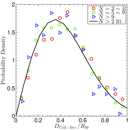
We choose to centre haloes on the iteratively-determined centres of light, which in most cases coincide with the locations of the BCGs. Although the existence of an offset between BCG and the real halo centre is well recognised (see,e.g., Skibba et al., 2011; Zitrin et al., 2012; George et al., 2012, and references therein), a reliable and general quantification of the offsets is not yet available. In order to estimate the prior distribution of offsets between projected mass and iteratively-determined centres of haloes, we start from investigating the displacements between different observational proxies of the halo centre. As shown in Figure 2, the displacement between the iteratively-determined and overall light centres in the real G³Cv5, when expressed in units of the group radius, $R_{50}\sim 0.2R_{200b}$, is almost independent of group observed mass or multiplicity. Its distribution can be well fitted with a 2D-Gaussian with mean 0 and $\sigma_{\tilde{\bf X}}=0.35$ in each dimension, where $\tilde{\mathbf{X}}=\mathbf{X}/R_{50}$. In Figure 2 only the distribution of $|\tilde{\bf X}|=D_{CoL-Iter}/R_{50}$ is plotted, which is a Rayleigh distribution (see Equation 27). Assuming the offset distributions of these two centres from the projected mass centre are independent and identical, this implies that $\sigma_{\tilde{\bf X}}=0.35/\sqrt{2}\simeq 0.2$. Hence we model the offset between observed and true halo centres with a Gaussian distribution having $\sigma_{\mathbf{X}}=0.2R_{50}$. The median, $\sigma_{\mathbf{X}}$, in our sample is $\sim 0.03\,h^{-1}\rm{Mpc}$, comparable with the estimation of $\sim 0.01\,h^{-1}\rm{Mpc}$ by Zitrin et al. (2012) for their SDSS cluster sample, and with the BCG offset of $\sim 0.02\rm{Mpc}$ estimated in George et al. (2012).

Figure 2: Distribution of the offset between the centre of light and the iterative centre for G³Cv5 groups. The separation between the two centres, $D_{CoL-Iter}$, is normalised by the comoving size, $R_{50}$, of each group. Different symbols represent different multiplicity ranges and the black solid line is a Rayleigh distribution fitted to the whole sample.

To estimate the distribution of the true halo mass at a given observationally-inferred mass, we make use of the mock G³C catalogues. In these, the true halo mass is well described by a log-normal distribution for any given dynamical (luminosity) mass measurement, with a dispersion $\sigma_{\log M}=0.6-0.8$ ($\sigma_{\log M}=0.5-0.7$), increasing (decreasing) with mass. For a measured luminosity mass in the range of $10^{13}-10^{15}h^{-1}\mathrm{M}_{\odot}$, which comprises the majority of our lenses, the dispersion stays roughly constant at $\sigma_{\log M}=0.5$, as is evident in the upper-right panel of Fig. 3. In what follows, we adopt $\sigma_{\log M}=0.5$ by default, but use $\sigma_{\log M}=0.7$ for the dynamical mass estimator.

Note that if the full likelihood function (Equation 25) is used, then in principle any parameters that are part of the distribution function can be fitted. For example, one would be able to measure the mean logarithmic halo mass, or the median mass parameter for the lognormal prior distribution in halo mass (Equation 28). As stated above, in this work we choose an alternative approach by fitting a simple likelihood function to the data ignoring the priors, and then calibrate the fitted parameters using random catalogues accounting for the priors. This is equivalent to the full likelihood fitting and, in the remainder of the paper, we will quote our calibrated best-fit mass-observable relations as the median mass-observable relation assuming a lognormal mass dispersion as in Equation (28).

4 Data analysis

4.1 Data cuts

In order to minimize systematic uncertainties, a series of cuts are applied to select the lens-source pairs for the likelihood analysis, as described below.

Closed-circle cut.

The model-noise correlation discussed in Section 3.4 is most significant on intermediate ($\sim 10$ Mpc) to large scales for our sample, but in this paper we are considering the small-scale matter distribution in and around haloes. Thus, instead of making any correction, we completely avoid this boundary effect by imposing a closed-circle cut. Specifically, when predicting the gravitational shear at the location of galaxy $s$, $\hat{\boldsymbol{\chi}}_{s}$, our model only includes contributions from lenses that are closer to the source than is the nearest survey boundary.

Virial cut.

We model each lensing group with a single NFW halo. However, on large scales the two-halo term, i.e., the matter distribution contributed by nearby haloes, dominates over the single halo term. Since our sample does not cover arbitrarily low mass haloes, our modelled matter distribution will be missing the contribution from low mass haloes that are not modelled. Hayashi & White (2008) showed that a sharp transition in the halo-mass cross-correlation, $\xi_{hm}$, happens at a scale where $\xi_{hm}\sim 6$, corresponding to $\sim 3R_{200b}$ for the halo mass and redshift ranges relevant here. Within this distance, the mass distribution is well described by a single halo profile. To avoid the correlation-dominated regime, we limit the analysis to within $2R_{200b}$ of each lens, where the virial radius $R_{200b}$ of the group is estimated from its luminosity mass. This cut essentially decouples the lens modelling of haloes from each other, except for close by ones. As we further discuss in Appendix B.2, the haloes that are not modelled should introduce a bias of less than $3\%$ in our mass estimates when our data cuts are applied.

Centre-offset cut.

If the iteratively-determined lens centre is offset from the projected centre of mass, then this will lead to an underestimate of the halo mass with the largest errors being made in the central density profile. To reduce any bias associated with this effect, lens-source pairs are not used where the source is within a projected distance $r_{p}=0.3R_{50}$ of a lens. This corresponds to a median physical radius of $\sim 0.04\,h^{-1}\rm{Mpc}$.

Obscuration cut.

It can be difficult to measure the shapes of background galaxies that lie close, in projection, to the bright central galaxies of foreground groups (e.g. Hirata et al., 2004; Mandelbaum et al., 2005a). Budzynski et al. (2012) found that the obscuration radius of SDSS DR7 galaxies is about 5 arcsec, so we exclude any source galaxy that lies within 10 arcsec of a foreground halo centre in our sample. Adopting an even larger cut of 20 arcsec makes no significant difference to our results.

Redshift cut

As a result of the large uncertainty in photometric redshift measurements, some foreground galaxies containing no real shear signal could be mistakenly identified as background source galaxies. To prevent excessive contamination from foreground galaxies, we only use source galaxies that have a photometric redshift at least $\Delta z=0.3$ higher than the spectroscopic redshift of the lens. This choice of redshift buffer is more conservative than the $\Delta z=0.1$ in Mandelbaum et al. (2006a), where they chose to correct for the remaining contamination with a boost factor. As there is a low lensing efficiency for small lens-source redshift separations, we estimate that our choice of the redshift buffer only reduces the signal-to-noise of the resulting measurements by $\sim 25\%$ compared to no buffering, while effectively removing all foreground galaxy contamination (see Appendix B.1). This large redshift cut also reduces systematics from the photo-z prior distributions, since $\Sigma_{\rm crit}$ is less sensitive to source redshift for larger redshift separations between lens and source.

Multiplicity cut.

As stated in Section 2, we only keep groups with three or more members as lenses by default. Note that this creates a multiplicity-limited sample whose mass-observable relations could generally differ from those in a volume-limited sample. To compare our results with thoeretical models properly, we will use mock catalogues with the same selection criteria as the observational sample. We discuss this selection effect further when we compare our measured mass-light relation and stellar mass-halo mass relation with other measurements in Sections 5.3, 5.4, and Appendix B.3.

4.2 Assessing systematics: Bias, Error and Significance

Random catalogues are used to calibrate the MLWL method for systematic errors introduced by the cuts applied to the data, described above, and the ignorance of prior distributions highlighted in Section 3.5. These catalogues are Monte Carlo realizations that also provide estimates of the statistical significance of our results. We will call them random catalogues, to differentiate from the galaxy mock catalogues described in Section 2.3, which are produced using a physically motivated galaxy formation model.

The random catalogues are based on the subsets of G³Cv5 groups and SDSS source galaxies that we are considering. For any lens, an observed mass is assigned from the parametrized mass-observable relation that we try to calibrate. True lens centres and masses are chosen for each group from the distributions given in Equations (27) and (28), while the source galaxies are assigned true redshifts via Equation (26) and “intrinsic” ellipticities according to a bivariate Gaussian with $\sigma=\sqrt{\sigma_{\chi}^{2}+\sigma_{SN}^{2}}$. This realisation of the source galaxy population is lensed by the set of inferred true lenses, ignoring the two-halo term, which is estimated to produce under 3% bias in our results (see Appendix B.2). Thousands of random catalogues were created, with all observational properties except source shapes being identical with those in the real data.

The same analysis procedure is applied to each random catalogue, adopting the same data cuts as were used with the real data, yielding distributions of the fitted parameters from the random catalogues. In all cases studied, the distributions can be reasonably well described by a normal distribution. For each parameter $x$ with mean, $\mu_{x}$, and standard deviation, $\sigma_{x}$, in the random catalogues, we derive its bias $\Delta_{x}=x_{0}-\mu_{x}$, where $x_{0}$ is the model input value. These derived biases and uncertainties are then applied to the parameters inferred from the real data, and we will quote our final measurements as

$$x=\hat{x}+\Delta_{x}\pm\sigma_{x},$$ (29)

where $\hat{x}$ is the best fit parameter value from the likelihood analysis on the real dataset. We leave the bias term explicitly in the result, because it depends on our assumptions of the prior distributions.

As explained in Section 3.4, in order to translate $TS$ to a significance value, one needs to know the distribution of $TS$ under the condition that the data are described by the null model. In the standard likelihood analysis, this is given by Wilks’s theorem, to be a $\chi^{2}_{n}(TS)$ distribution. However, our $TS$ is estimated from a simple likelihood model which is only a crude description of the data distribution, because the prior distributions are ignored in the simple model. This invalidates Wilks’s theorem. The distribution of our estimated $TS$ is therefore expected to differ from $\chi^{2}_{n}(TS)$, and we calibrate this distribution using our random catalogues. As in Han et al. (2012), we find that the $TS$ distribution in the presence of systematics no longer follows a $\chi^{2}_{n}(TS)$ distribution. However, when scaled as $TS^{\prime}=TS/b$, where $b$ is a consant to be determined, $TS^{\prime}$ can be very well described by a $\chi^{2}_{n}(TS^{\prime})$ distribution with the same number of degrees of freedom. In what follows, instead of interpreting $TS$ by reference to a $\chi^{2}_{n}(TS/b)$ distribution, we will make use of $TS^{\prime}=TS/b$ which behaves as a standard $\chi^{2}_{n}$ variable. This $TS^{\prime}$ serves as a “corrected” $TS$ and can be used to obtain significance levels using conventional $\chi^{2}_{n}$ distributions. By fitting the $TS$ distribution in the random catalogues with a $\chi^{2}_{n}(TS/b)$ distribution, we can derive the scale factor $b$ and use it to correct the observed $TS$ in the real measurements.

5 Results and Discussion

In this section we describe in detail our measured mass-observable relations, and compare these results with those in previous studies. As mentioned in the beginning of Section 3, we will be taking two complementary approaches in our fitting: 1) splitting the whole sample into several bins according to some observable and fitting a single mass to all the haloes within each bin; 2) predicting the mass of each halo from a mass-observable relation and fitting for the parameters of this relation globally. While the former approach is able to give a non-parametric description of the mass-observable relations, the latter uses all the lenses more efficiently and yields analytical descriptions of the relations. We summarize these parametrized fits in Table 1, along with an estimated bias and uncertainty inferred from random catalogues, in the form of Equation (29). We also list the correlation coefficients, estimated from the likelihood surface between parameters from the fitting, as well as the $TS$ with respect to a null model with no gravitational shear. A visualization of the halo density profiles through stacked lensing is provided in Appendix D. Since we will be showing the best fits together with systematic corrections throughout the following sections, we first provide an overview of those systematic corrections.

5.1 Overview of the systematic corrections

Systematic corrections to the fits are derived following the procedure detailed in Section 4.2 by applying our likelihood fitting to random catalogues that account for the prior distributions described in Section 3.5. After incorporating these additional stochastic processes in the random catalogues, the derived errors are generally larger than those estimated from direct likelihood fitting of the real data. The systematic biases barely affect the power-law slopes in our models, and are generally smaller than the parameter uncertainties.

We use the random catalogues to check for effects of both the data cuts and the prior distributions. To check the effect of the data cuts alone, we first create two sets of random catalogues with no prior distributions. In generating these catalogues, one set has the same data cuts as in Section 4.1 when predicting the shear field, while the other set has no data cuts at all. In both cases, the true parameters and their errors are accurately recovered from direct likelihood fitting on the random catalogues. This confirms that our adopted data cuts do not bias the results, and that our MLWL method is working well when no systematics from prior distributions are present. To calibrate the effect of the priors, we generate one set of random catalogues for each mass-observable relation that we wish to calibrate. Direct likelihood fitting is performed on these catalogues with no priors in the model, and the bias and error of the fitted parameters are extracted from their distributions after the fitting.

To see the separate effects of photo-$z$, centre-offset and mass-dispersion on the fitting, we generate one additional set of mocks including each effect individually for the last model in Table 1, $M=AM_{\rm lum}$, and assess their biases. This yields $\Delta_{\log(A)}=0.02,0.08,-0.17$ for photo-$z$, centre-offset and mass-dispersion biases respectively, revealing that one tends to underestimate the mass when ignoring photo-$z$ bias and centre-offset effects, while overestimating the mass by assuming there is no dispersion in the mass-observable relation. Our estimated photo-$z$ bias translates into $-5$ per cent in mass, in good agreement with that obtained by Nakajima et al. (2012) at our median group redshift $z=0.2$ ( assuming $M\propto\Delta\Sigma^{1.5}$; see Mandelbaum et al., 2010). Mandelbaum et al. (2005b) found that the stacked lensing-estimated mass lies in between the mean and median value of the actual mass of the sample in the presence of a mass scatter. This is consistent with our result that for a log-normal mass scatter, the estimated mass is higher than the median (or the mean in $\log M_{h}$). Note that the overall bias $\Delta_{\log(A)}=-0.09$ is roughly the summation of the three, but is dominated by the mass dispersion bias. Assuming a mass dispersion of 0.7 dex would lead to $\Delta_{\log(A)}=-0.32$. In Table 1 we adopt a mass dispersion of 0.5 dex by default, and use 0.7 dex for the dynamical mass estimators (marked by ${\dagger}$ in the table), leading to larger biases in their parameters.

Figure 3: Halo mass scaling with observed group properties. The upper-left panel contains the dependence of group mass on redshift, showing the selection in our sample. The other three panels show the scaling of halo mass with $r$-band group luminosity, $L_{\rm grp}$, multiplicity volume, $V_{N}$, and stellar mass of the central galaxy, $M_{\star}$. In each panel, the data points with errorbars show the halo mass measured using MLWL within each observable bin. The vertical errorbars are estimated from the weak lensing likelihood, while the horizontal errorbars simply mark the span of each bin. Black solid lines are the globally fitted power-law scalings from the MLWL method. The black dashed lines show the global fits after systematic correction (except in the redshift dependence panel). Note we have not applied systematic corrections to the binned measurements. Green solid lines depict the median relation extracted from 9 mock GAMA catalogues, while the green dashed lines mark the typical 16th and 84th (i.e., $\pm 1\sigma$) percentiles of the halo mass distribution in one mock catalogue.

5.2 Mass-Observable Scaling Relations

Figure 4: Halo mass scaling with group velocity dispersion, $\sigma_{v}$, and observed radius, $R_{50}$. $R_{50}$ is defined to be the projected radius containing $50\%$ of the observed galaxies in the group. Line styles are the same as in Fig. 3. The vertical black dashed line in the $M_{h}(R_{50})$ panel marks the spatial resolution of the Millennium simulation underpinning the mocks.

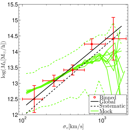
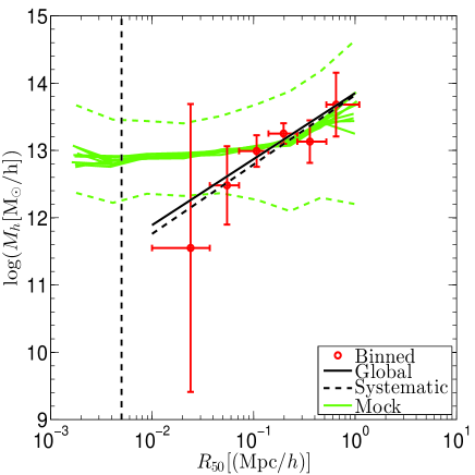
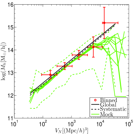
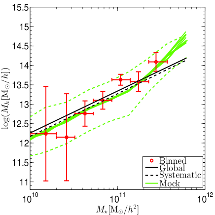
Before parametrizing the mass-observable relations with particular functional forms, we can measure them in a non-parametric way by splitting the lens sample according to a single mass proxy. We fit a single mass parameter to each subsample of lenses. These measurements will provide a consistency check with the parametrizations adopted in our global fits. Unlike stacked lensing, we still do maximum likelihood fitting over every source galaxy after splitting the lens sample. As a result of our virial cut, the different lenses are mostly decoupled from each other, and it makes little difference whether we fit the bins jointly or independently. For the same reason, we expect the systematic correction to each binned measurement to be the same as that obtained for the global fit. In addition, because we present the binned measurements mostly to reassure that our parametrizations of the mass-observable relations are reasonable, and because it is computationally expensive to estimate the systematic corrections, we make no attempt to derive the corrections for the binned measurements.

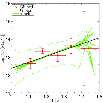
In Figs 3 and 4 we explore the scaling relations for various mass observables: group velocity dispersion, $\sigma_{v}$; group total luminosity, $L_{\rm grp}$; stellar mass of the iterative central galaxy, $M_{*}$; the multiplicity volume, $V_{N}$; and the observed radius, $R_{50}$. Note that the total luminosity has been corrected for unobserved galaxies in the group by integrating the GAMA galaxy luminosity function.

A similar correction can be done for the observed multiplicity of groups, $N$, to derive an absolute multiplicity $N_{\rm abs}$. Equivalently, we choose to introduce a multiplicity volume as

$$V_{N}=\frac{N}{n(z)},$$ (30)

where $n(z)$ is the average number density of observed galaxies at redshift $z$. This volume translates into $N_{\rm abs}$ when multiplied by the expected number density of galaxies down to the desired absolute magnitude limit. Even though group redshift is not a physical mass proxy, we still include it in Fig. 3 to show the group sample selection varies with redshift.

Figure 5: The scaling of group luminosity with velocity dispersion, $\sigma_{v}$, and size, $R_{50}$. In both panels, the solid lines show the median group luminosity at fixed $\sigma_{v}$ or $R_{50}$, while the dashed lines plot the 16th and 84th (i.e., $\pm 1\sigma$) percentiles. The red thick lines represent the results from the GAMA group catalogue, while the green thin lines are those from the mocks. Note that for the mocks we have plotted one median line for each mock catalogue, but only one set of $\pm 1\sigma$ percentiles. In the $L_{\rm grp}(R_{50})$ panel, the vertical black dashed line marks the spatial resolution of the Millennium simulation underpinning the mocks.

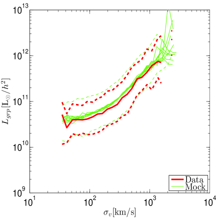
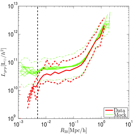
All of these scaling relations can be well described by power-law functions. Hence we provide global fits of these relations by modelling the mass of each group as a power-law function of a single observable of the group, and maximizing the likelihood of the entire sample. This produces the parametrized relations in Table 1, which are shown with black lines in Figs 3 and 4. As expected they all agree with the binned measurements. For each fit (except that for the redshift selection), we also plot a dashed line showing the relation after applying the systematic correction listed in Table 1.

In Figs 3 and 4 we also compare our measurements with predictions from mocks. From each of 9 mocks, we extract the 16th, 50th and 84th percentiles of the halo mass distribution as functions of the group properties. The measured redshift evolution of the halo mass agrees well with that determined from the mocks, reflecting the identical redshift selection in the real and mock catalogues. Both the measured $M_{h}(L_{\rm grp})$ and $M_{h}(V_{N})$ relations agree remarkably well with those in the mocks. The former may not be too surprising since the semi-analytical model underlying the mocks is tuned to reproduce the galaxy luminosity function. In addition, a further adjustment has been made to the galaxy luminosities in the mocks, attributing any residual difference in the redshift-dependent luminosity distribution to survey photometry. However, these adjustments are guided by the global luminosity function, while our measurement probes the halo occupation distribution (HOD) of the galaxies, revealing that the mocks have correctly populated haloes with (total) light. According to our definition, $V_{N}$ is a measurement of the average clustering of galaxies out to group boundaries. If one assumes that galaxies trace the distribution of dark matter with a constant bias, then $V_{N}\sim(4\pi/3)\Delta R_{200b}^{3}$ where $\Delta=200$ according to our virial convention. Thus, one expects $M\propto V_{N}$, which is what we see in Fig. 3, where the global fit gives $M_{h}\propto V_{N}^{1.03+0.01\pm 0.23}$. This agreement with the mocks indicates that we have correctly modelled the average spatial distribution of galaxies inside and outside groups. The measured $M_{h}(M_{\star})$ relation also agrees quite well with the mock predictions.

The globally fitted $M_{h}(\sigma_{v})$ relation is slightly steeper than that seen in the mocks. This difference is too large to be accounted for by the anticipated systematic error in the slope, and persists when we use only $N>5$ groups. Examination of the binned measurement shows that the difference originates from the lower measured mass at low $\sigma_{v}$ and higher measured mass at high $\sigma_{v}$. In both of these regimes, the uncertainties are much larger than those at intermediate velocity dispersion due to either intrinsically small halo mass or the small number of stacked groups at high mass. Overall, the measurement is marginally consistent with the mock predictions according to the error bars. The small tension may originate from a velocity bias of satellite subhaloes in the dark matter-only Millennium simulation. For example, Munari et al. (2013) find that while galaxies trace dark matter closely in SPH simulations, the velocity dispersions of subhaloes in simulations with cooling are generally lower than those in dark matter-only or adiabatic simulations, due to the longer survival times for low velocity subhaloes in the former. The situation is further complicated by the existence of “orphan” galaxies in semi-analytical models, i.e. galaxies whose associated dark matter substructure has become unresolved in the simulation. In this case, the galaxy position is chosen to be that of the most bound particle from the previously associated subhalo. This results in a velocity distribution that follows that of the dark matter particles. However, as found in Munari et al. (2013), there is a halo mass dependent velocity dispersion bias between the subhaloes and dark matter particles. This could have given rise to the different $M-\sigma_{v}$ slope we see in the mock. A similar discrepancy is observed for the $M_{h}(R_{50})$ relation as well, but only at small $R_{50}$, where the predicted halo mass is almost constant while the measured mass keeps decreasing with $R_{50}$. Despite this difference, the prediction is still marginally consistent with the measurements within the error ranges.

If the $M_{h}(\sigma_{v})$ and $M_{h}(R_{50})$ scaling relations are indeed different in the data and in the mocks, then one might expect different scaling of $L_{\rm grp}$ with $\sigma_{v}$ or $R_{50}$ as well, since we have seen that $L_{\rm grp}$ is a good halo mass proxy in both real and mock data. We compare these light-observable relations in Fig. 5. While there is little to distinguish between the real and mock $L_{\rm grp}(\sigma_{v})$ relations, there is an obvious difference in the $L_{\rm grp}(R_{50})$ scaling between the two, similar to the difference observed in the $M_{h}(R_{50})$ relation. Note that this difference is most pronounced near the spatial resolution $\epsilon=5h^{-1}\rm{kpc}$ of the Millennium simulation underpinning the mock catalogues, but is still observable out to $R_{50}\sim 40\epsilon$. Similar results have been found when measuring the galaxy correlation function, where the autocorrelation function of red galaxies on small scales in the GAMA mocks significantly exceeds that in the real data (Farrow, 2013). This discrepancy ties in with studies of the radial distribution of satellite galaxies, which find an overprediction of model red satellites (Budzynski et al., 2012; Guo et al., 2013; Wang et al., 2014). Our result is also in line with Robotham et al. (2011) who find an overprediction of the number of compact groups in the mocks.

The discrepancy between mock and data compact group luminosities could also be due to a selection effect caused by imperfections in the SDSS photometry. As the GAMA input catalogue was constructed from the SDSS photometric galaxies, selection effects in the latter could propagate to the GAMA catalogue. It is known that near bright galaxies, the flux level of the background sky could be overestimated in the SDSS(Adelman-McCarthy et al., 2008), leading to an underestimate of the flux of neighbouring galaxies. As a result, faint galaxies in the vicinity of bright ones could be missing from the flux-limited GAMA galaxy catalogue, which in turn could remove bright and compact groups from the group catalogue. Note this type of selection is not implemented in the current GAMA mock catalogues, which could result in an excess of bright groups at small $R_{50}$ compared to observations.

The model’s treatment of orphan galaxies, which dominate the galaxy population in the inner halo, may also be responsible for the differences between model and data $M_{h}(\sigma_{v})$ and $M_{h}(R_{50})$ relations. Changes in how the positions of these galaxies are modelled, and in the dynamical friction time estimation can both affect the satellite abundance and hence the size distribution of sample groups. For example, Jiang et al. (2008) found that the dynamical friction time scale inferred by Bower et al. (2006) is overestimated for major mergers, resulting in an excess of orphan galaxies in the model. Lastly, when constructing the light-cone mocks, it is necessary to interpolate the position and velocity of galaxies between simulation snapshots in order to place galaxies in an observer’s past light cone. Even though Merson et al. (2013) have tried several different interpolation methods, we do not exclude the possibility that those interpolations could distort the spatial and velocity distributions of galaxies, contributing to our observed discrepancies.

5.3 Comparison of group mass to light ratio with 2PIGG measurement

Figure 6: The mass-to-light ratio of groups. In the left-hand panel, the points with error bars are the MLWL fitted $M_{h}/L$ within each luminosity bin. A green solid line shows the median $M_{h}/L$ at fixed luminosity in the mocks, while the green dashed lines are the 16th and 84th (i.e., $\pm 1\sigma$) percentiles. The blue thick line is the 2PIGG-inferred $M_{h}/L$ (Eke et al., 2004b). The right-hand panel is like the left, just with the groups in both real and mock samples further selected to mimic the 2PIGG selection function. The red dashed line is an unbinned broken power-law fit of the form $M_{h}/L=A\min(L_{\rm grp}/L_{p},1)^{b}$.

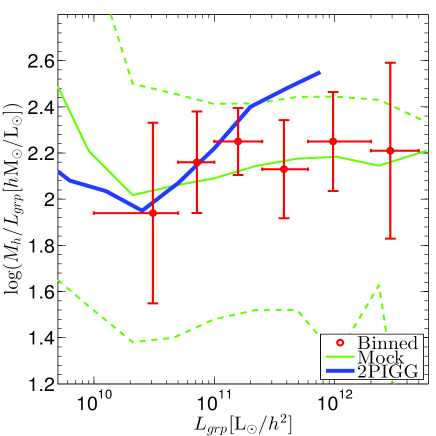
In the left-hand panel of Fig. 6, we compare the measured group mass-to-light ratios with those from the 2 degree Field Galaxy Redshift Survey (2dFGRS, Colless et al., 2001) Percolation-Inferred Galaxy Group catalogue (Eke et al., 2004b, 2PIGG hereafter). The mass-to-light ratios in 2PIGG are derived from group dynamical masses and $r_{F}$ band total luminosities. We have calibrated their $r_{F}$ band luminosity to $r$ band in the comparison. This time our measurement from the G³Cv5 is done by fitting a constant $M_{h}/L$ value to all groups within each luminosity bin. For the mocks, we measure the median and 16th and 84th (i.e., $\pm 1\sigma$) percentiles of $M_{h}/L$ within each luminosity bin. Again our measured $M_{h}/L$ agrees very well with the mock prediction. Below $L_{\rm grp}=2\times 10^{11}h^{-2}\mathrm{L}_{\odot}$, it appears that our measurement is also in good agreement with that from the 2PIGG catalogue. However, for brighter groups, our measured $M_{h}/L$ stays almost constant, while the 2PIGG $M_{h}/L$ continues to increase with $L_{\rm grp}$. This difference can be largely explained by the different depths of the two surveys. Since groups are selected to have a minimum number of $N_{\rm min}$ galaxies in both catalogues, the group selection function can be described as

$$V_{N}^{\rm lim}(z)=N_{\rm min}/n_{<M_{\rm lim}(z)},$$ (31)

where $n_{<M_{\rm lim}(z)}$ is the number density of galaxies above the survey flux limit. As the GAMA survey is $\sim 2$ magnitudes deeper than the 2dFGRS, we expect 2PIGGs to behave like poorly sampled GAMA groups. Note that the completeness of the 2dFGRS is not as uniform as in GAMA, so the estimated $n_{<M_{\rm lim}(z)}$ varies across the sky. We model this $n_{<M_{\rm lim}(z)}$ with a Gaussian distribution at given $z$, and generate a random $n_{<M_{\rm lim}(z)}$ for each GAMA group at $z$ to account for the variation of completeness in the 2dFGRS. Repeating the $M_{h}/L$ calculation on a sub-sample of our groups selected with the 2dFGRS depth, $V_{N}>V_{N}^{\rm lim,2dF}$, which constitutes $\sim 1/3$ of our standard sample, gives the results in the right-hand panel of Fig. 6. Due to the reduced signal-to-noise, we also show an unbinned broken power-law fit of the form $M/L=A\min(L_{\rm grp}/L_{p},1)^{b}$, where $L_{p}$ and $b$ are the parameters to be fitted. Using the 2dFGRS selection function decreases the measured $M_{h}/L$ at low $L_{\rm grp}$ due to the inclusion of $N=2$ groups, while that at high $L_{\rm grp}$ is increased due to the exclusion of low $V_{N}$ groups at given redshift. This time our measurement largely agrees with the 2PIGG result for groups around $L_{\rm grp}=3\times 10^{11}h^{-2}\mathrm{M}_{\odot}$, showing the importance of sample selection when comparing observed group properties with other results.

5.4 Comparison of the halo mass-stellar mass relation with other works

Figure 7: The measured halo mass-stellar mass relation compared with several HOD prescriptions and mock predictions. In both panels, the red circles with error bars are the MLWL measured $M_{h}(M_{\star})$ relation for multiplicity $N>2$ groups, and the red solid line is the median relation for $N>2$ groups in the mocks. In the left-hand panel, the dashed lines are the converted $M_{h}(M_{\star})$ relations from the various HOD distributions. From top to bottom on the top-right corner, they are Guo et al. (2010)(blue), Moster et al. (2013)(green), Wang et al. (2013a)(cyan) and Wang et al. (2013b)(grey). In the right-hand panel, the black squares with errorbars are the measured relation for a volume-limited central galaxy sample that is complete up to $z=0.2$ and covers central galaxies down to $N=1$. The black dashed line is the median relation for the central galaxies in the mock, similarly selected to be volume limited. A yellow band shows the range of converted $M_{h}(M_{\star})$ relations from the four HOD models when a common dispersion of $\sigma_{\log(M_{\star})}=0.2$ is adopted.

Figure 8: The redshift distribution of central galaxies inside different stellar mass bins. The sample covers all the central galaxies in groups down to $N=2$, and all the ungrouped galaxies down to $r_{AB}<19.4$. Different coloured lines represent different stellar mass bins, with increasing stellar mass from top to bottom at $z<0.2$. The binning in stellar mass is the same as used in Fig. 7. Up to $z=0.2$, all the stellar mass bins are complete, except for a slight incompleteless in the smallest mass bin.

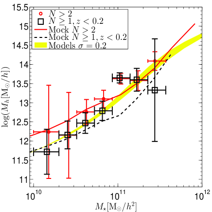
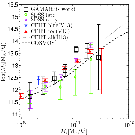
The measured $M_{h}(M_{\star})$ is compared with several recent halo occupation distribution (HOD) descriptions for group central galaxies in Fig. 7. We calibrate the units and mass definitions in these relations to those used here, and list them in Table 2 along with the dispersion in stellar mass at fixed halo mass used for each of these studies. Note that all the average $M_{\star}(M_{h})$ relations in these HOD descriptions are measuring the median stellar mass of the central galaxy for haloes of a given mass. What we measure is the median halo mass for groups of a given central stellar mass, assuming a log-normal distribution in halo mass at fixed central stellar mass. To make the HOD-based relations comparable with our measurements, we make use of

$$dP(M_{h}|M_{\star})=\frac{dP(M_{\star}|M_{h})\phi(M_{h})dM_{h}}{\int dP(M_{\star}|M_{h})\phi(M_{h})dM_{h}},$$ (32)

where $\phi(M_{h})=dN(M_{h})/dM_{h}$ is the halo mass function. When $dP(M_{\star}|M_{h})$ follows a log-normal distribution, as is assumed when the HOD-based relations are inferred, we find that the converted distribution, $dP(M_{h}|M_{\star})$, is also very well described by a log-normal distribution, consistent with what had been assumed in Equation (28). The median halo mass, or mean logarithmic mass, can then be found through

$$\log M_{h}(M_{\star})=\int\log(M_{h})dP(M_{h}|M_{\star}).$$ (33)

We adopt the Sheth et al. (2001) mass function in our conversion, and have checked that adopting the Tinker et al. (2008) mass function or a different cosmology (Millennium/WMAP9/Planck) produces no more than a $10\%$ difference in the converted relations at the high mass end, much smaller than model to model variations.

At low masses ($M_{\star}<10^{11}h^{-2}\mathrm{M}_{\odot}$), it appears that the Guo et al. (2010) and Moster et al. (2013) results agree best with our measurement for groups with more than two members, while at the high mass end the average halo mass in our sample is lower than their predictions. However, we emphasize that our standard sample is limited to groups with three or more members. This introduces a redshift dependent selection in $V_{N}$, given by $V_{N}^{\rm lim}(z)=N_{\rm min}/n_{<M_{\rm lim}(z)}$. Since $V_{N}$ is strongly correlated with halo mass, in principle all our measured relations could be biased with respect to the relation in a volume limited halo sample. We have tested a different multiplicity cut of $N>5$, and it does give a systematically higher $M_{h}(M_{\star})$ relation. In Appendix B.3 we explicitly show how the halo mass depends on $N_{\rm abs}$ at fixed $M_{\star}$ or $L_{\rm grp}$ in a volume limited mock catalogue. With the knowledge that our observed halo mass-stellar mass relation is strongly multiplicity dependent, including central galaxies from $N<3$ groups will only lower our measurement. To derive a selection-free stellar mass (SM)-halo mass (HM) relation, we extend our sample to include $N=2$ groups as well as ungrouped galaxies representing $N=1$ groups. This gives us a flux-limited central galaxy sample. As we show in Fig. 8, by further restricting to $z<0.2$, we get a volume limited sample of central galaxies with $M_{\star}>10^{10}h^{-2}\mathrm{M}_{\odot}$. The measured halo masses are shown with black squares in the right-hand panel of Fig. 7. We also show the median halo mass for mock galaxies with the same selection. The match between data and mocks improves slightly if we shift the measured halo masses down by $0.07$ dex, the typical size of systematic correction estimated in Table 1.

The quoted HOD models, though differing substantially in their predicted stellar mass for a given halo mass, all give a satisfactory fit to the stellar mass function with their adopted dispersions. Hence, deriving the SM-HM relation from pure abundance matching inevitably faces a degeneracy between the average SM-HM relation and the SM dispersion at fixed HM (see, e.g., Wang et al., 2006).

We find the converted relation is more sensitive to the model dispersion than to the mean relation. We show in the right panel of Fig. 7 that when a common dispersion value is adopted, all of the converted relations are very similar. With $\sigma_{\log(M_{\star})}=0.2$, the volume-limited measurement can be well reproduced by any of the HOD models. This is consistent with the values of $0.16-0.2$ dex found by many previous works (e.g., Yang et al., 2009; Li et al., 2012; Leauthaud et al., 2012; Reddick et al., 2013; Behroozi et al., 2013; Kravtsov et al., 2014). Note this dispersion includes both the intrinsic stellar mass variation at a given halo mass and the stellar mass measurement error. Subtracting the typical stellar mass measurement error of $0.13$ dex for our sample, the intrinsic dispersion is found to be $\sigma_{\log(M_{\star}),{\rm intrinsic}}\sim 0.15$.

In Figure 9, we compare our SM-HM relation derived from the volume limited sample to that measured in several other galaxy-galaxy lensing studies, including the measurements in SDSS (Mandelbaum et al., 2006b), CFHTLenS (Velander et al., 2013; Hudson et al., 2013) and COSMOS (Leauthaud et al., 2012). As in Figure 7, we plot the average logarithmic halo mass at fixed stellar mass. The halo mass definitions are either in or converted to our $M_{200b}$ convention according to the scaling relation in Giocoli et al. (2010), except for the SDSS measurements which adopt $M_{180b}$. The difference between $M_{200b}$ and $M_{180b}$ is only around $3$ percent, so we do not correct for it here. The COSMOS result is provided in the form of a HOD model, which we have converted to our convention according to Equations (32) and (33). CFHTLens results are given by Velander et al. (2013) and Hudson et al. (2013) independently. To avoid overcomplicating the figure, in the case of Hudson et al. (2013) we only plot their best-fit relation for the full sample evaluated at $z=0.3$, the redshift of their lowest redshift bin.

It is worth noting that our measurements are based on a sample of central galaxies, while others use samples mixing both central and satellite galaxies. They all rely on HOD modelling to extract a stellar mass-halo mass relation, typically mixing both populations. They can still differ in how satellite galaxies are modelled. In the COSMOS model, a satellite galaxy has no subhaloes, and contributes to the lensing signal only through the displaced density profile of its host halo. In the other three studies shown in Fig. 9, satellites are associated with subhaloes with truncated density profiles, parametrized by a halo mass parameter that follows the same stellar mass-halo mass relation as that of the central galaxies. One should also note that while both the SDSS and our lens samples have spectroscopic redshifts, the CFHTLens and COSMOS lens samples rely on photometric redshifts. Lastly, we point out that both our stellar mass sample and the COSMOS sample are volume-limited, unlike the other samples being considered here, which are flux-limited and hence subject to stellar mass incompleteness. However, we find little difference in our results between flux-limited and volume-limited samples. Overall, despite the different methods and datasets, good agreement is found among the various results considered here.

Note that our measured masses may be systematically ($0.1-0.2$ dex) above the median halo mass of the underlying distribution at a fixed stellar mass, primarily as a consequence of the scatter in the $M_{h}(M_{*})$ relation. A correction for this would bring our measurements closer to the COSMOS line. Similar corrections are already included in the quoted relations from the other studies, except for Hudson et al. (2013). It is worth emphasizing that this correction refers to the difference between the best-fitting mass and the median mass of the stacked haloes in each stellar mass bin, but not the Bayesian conversion between $<M_{*}|M_{h}>$ and $<M_{h}|M_{*}>$ (i.e, Equation (32)). In Hudson et al. (2013), even though the Bayesian conversion is performed when fitting a parametric SM-HM relation, the correction from the best-fit lensing mass to the median mass is not given. In some other works, for example when the COSMOS measurement is compared with that from the CFHTLens in Velander et al. (2013) and with SDSS measurements in Leauthaud et al. (2012), the Bayesian conversion is not carried out, resulting in an apparent discrepancy between the COSMOS result and other measurements at the high mass end.

There could also be systematic uncertainties in the stellar mass estimates across different studies. Mandelbaum et al. (2006a) adopt a Kroupa IMF in the stellar mass estimate, while all the others assume a Chabrier IMF. The difference in stellar mass caused by these two IMFs is typically $0.05$ dex. However, one should keep in mind that the systematic uncertainties in stellar mass estimates can be as large as $0.25$ dex, depending on the detailed implementation of the stellar population synthesis models (Behroozi et al., 2010).

Finally, we note that the general trend observed between halo and stellar mass in this work is similar to those obtained in, e.g., Lin & Mohr (2004); Lin et al. (2004); Zheng et al. (2007); Brown et al. (2008); Guo et al. (2014); Oliva-Altamirano et al. (2014), using a variety of methods and galaxy samples.

Figure 9: The central halo mass-stellar mass relation measured from weak lensing. We compare our measurements derived from the volume limited stellar mass sample to several other galaxy-galaxy lensing measurements, including from SDSS (split according to early and late types; Mandelbaum et al., 2006b), CFHTLenS (split according to colour by Velander et al., 2013, V13, or a fit to the full sample Hudson et al., 2013, H13), and COSMOS (Leauthaud et al., 2012, $z\sim 0.37$). As in Figure 7, we plot the average logarithmic halo mass at fixed stellar mass. The COSMOS measurement and is provided as a fitted $<\log(M_{\star})|M_{h}>$ relation, which we have converted to our convention according to Equations (32) and (33). The same conversion is done for the results from Hudson et al. (2013).

Table 1: MLWL Calibrated Mass-Observable Relations. The parameter values are listed as $x=\hat{x}+\Delta_{x}\pm\sigma_{x}$, where $\hat{x}$, $\Delta_{x}$ and $\sigma_{x}$ are the best-fitting value, bias and error for parameter $x$. $TS$ is the test statistic defined in Equation (23), where the null model is the one with no gravitational shear. In general a larger $TS$ means a better fit. Additional systematic uncertainties can lead to reduced $TS$ values, and a dilution factor $b$ is estimated to account for these uncertainties. We list the test statistic together with its estimated dilution factor $b$ as $TS/b$. The significance value is derived from the $TS$ value, taking into account the degrees of freedom in the fitting, and describes how significantly the best-fit differs from statistical fluctuations of the null model. We derive the significances for both the raw $TS$ and the diluted $TS/b$, and list the diluted significance in parenthesis beside the raw significance. In estimating the parameter bias, we adopt a mass dispersion of 0.5 dex by default, but use 0.7 dex for the dynamical mass estimators (marked with †), leading to larger estimated biases in their parameters. The power-law pivot scales are: $M_{0}\equiv 10^{14}h^{-1}\mathrm{M}_{\odot}$, $M_{*0}\equiv 10^{11}h^{-2}\mathrm{M}_{\odot}$, $L_{0}\equiv 2\times 10^{11}h^{-2}\mathrm{L}_{\odot}$, $v_{0}\equiv 500\,{\rm km\,s}^{-1}$, $V_{0}\equiv 1000(h^{-1}\mathrm{Mpc})^{3}$, $R_{0}\equiv 0.3h^{-1}\mathrm{Mpc}$. $M_{p}$ is in units of $h^{-1}\mathrm{M}_{\odot}$, while $A$ is dimensionless. $M_{\rm dyn}$ and $M_{\rm lum}$ refer to the G³Cv5 mass estimator defined in Equation (1) and (2). The $\log()$ function is base 10 throughout this paper. $C$ represents the correlation coefficient, inferred from the Hessian matrix of the log-likelihood, for the two parameters listed as subscripts. Note these results are derived from a flux-limited group catalogue (G³Cv5) and are subject to the group selection function.

Halo Mass Estimator	Fitted Parameters	Parameter correlation	$TS/b$	Significance	Reference
$M_{p}\left(\frac{V_{N}}{V_{0}}\right)^{\alpha}$	$\log(M_{p})=13.58-0.07\pm 0.13$ $\alpha=1.03+0.01\pm 0.23$	$C_{\log(M_{p})\alpha}=0.18$	46.1/1.5	6.5(5.1)	Fig. 3
$M_{p}\left(\frac{L_{\rm grp}}{L_{0}}\right)^{\alpha}$	$\log(M_{p})=13.48-0.08\pm 0.12$ $\alpha=1.08+0.01\pm 0.22$	$C_{\log(M_{p})\alpha}=-0.16$	53.9/2.2	7.0(4.6)	Fig. 3
$M_{p}\left(\frac{M_{*}}{M_{*0}}\right)^{\alpha}$	$\log(M_{p})=13.34-0.07\pm 0.12$ $\alpha=1.08+0.02\pm 0.28$	$C_{\log(M_{p})\alpha}=0.07$	42.7/1.4	6.2(5.2)	Fig. 3
†    $M_{p}\left(\frac{\sigma_{v}}{v_{0}}\right)^{\alpha}$	$\log(M_{p})=13.67-0.21\pm 0.08$ $\alpha=2.09+0.08\pm 0.34$	$C_{\log(M_{p})\alpha}=0.32$	46.9/5	6.5(2.6)	Fig. 4
$M_{p}\left(\frac{R_{50}}{R_{0}}\right)^{\alpha}$	$\log(M_{p})=13.34-0.06\pm 0.13$ $\alpha=0.98+0.05\pm 0.38$	$C_{\log(M_{p})\alpha}=0.49$	32.6/1.4	5.4(4.4)	Fig. 4
$M_{p}\left(\frac{\sigma_{v}}{v_{0}}\right)^{\alpha_{\sigma}}\left(\frac{V_{N}}{V_{0}}\right)^{\alpha_{V}}$	$\log(M_{p})=13.78-0.07\pm 0.17$ $\alpha_{\sigma}=1.28+0.00\pm 0.45$ $\alpha_{V}=0.61+0.02\pm 0.24$	$C_{\log(M_{p})\alpha_{\sigma}}=0.24$ $C_{\log(M_{p})\alpha_{V}}=-0.05$ $C_{\alpha_{\sigma}\alpha_{V}}=-0.65$	54.6/1.7	6.8(5.0)	Fig. 11
$M_{p}\left(\frac{L_{\rm grp}}{L_{0}}\right)^{\alpha_{L}}\left(\frac{V_{N}}{V_{0}}\right)^{\alpha_{V}}$	$\log(M_{p})=13.31-0.03\pm 0.28$ $\alpha_{L}=1.99-0.10\pm 0.98$ $\alpha_{V}=-0.92+0.10\pm 0.90$	$C_{\log(M_{p})\alpha_{L}}=-0.73$ $C_{\log(M_{p})\alpha_{V}}=0.74$ $C_{\alpha_{L}\alpha_{V}}=-0.95$	56.2/1.6	6.9(5.3)	Fig. 11
$M_{p}\left(\frac{L_{\rm grp}}{L_{0}}\right)^{\alpha_{L}}\left(\frac{\sigma_{v}}{v_{0}}\right)^{\alpha_{\sigma}}(1+z)^{\alpha_{z}}$	$\log(M_{p})=14.15-0.07\pm 0.30$ $\alpha_{L}=0.78+0.02\pm 0.29$ $\alpha_{\sigma}=1.31+0.03\pm 0.52$ $\alpha_{z}=-5.79+0.18\pm 3.64$	$C_{\log(M_{p})\alpha_{L}}=-0.20$ $C_{\log(M_{p})\alpha_{\sigma}}=0.53$ $C_{\log(M_{p})\alpha_{z}}=-0.91$ $C_{\alpha_{L}\alpha_{\sigma}}=-0.67$ $C_{\alpha_{L}\alpha_{z}}=0.01$ $C_{\alpha_{\sigma}\alpha_{z}}=-0.37$	63.7/2.4	7.2(4.2)	Fig. 11
†    $A\left(\frac{M_{\rm dyn}}{M_{0}}\right)^{\alpha}M_{\rm dyn}$	$\log(A)=-0.54-0.22\pm 0.10$ $\alpha=-0.31+0.04\pm 0.15$	$C_{\log(A)\alpha}=0.12$	43.9/5.3	6.3(2.4)	Fig. 10
$A\left(\frac{M_{\rm lum}}{M_{0}}\right)^{\alpha}M_{\rm lum}$	$\log(A)=-0.28-0.07\pm 0.12$ $\alpha=-0.01+0.01\pm 0.19$	$C_{\log(A)\alpha}=0.28$	52.2/1.9	6.9(4.9)	Sec. 6.1
$AM_{\rm lum}$	$\log(A)=-0.28-0.09\pm 0.09$	-	52.2/2.2	7.2(4.9)	Sec. 5.1; Fig. 10

6 Calibration and Construction of Mass Estimators

In this section we apply our MLWL method to calibrate the existing halo mass estimators from the G³Cv5 catalogue. We also try to construct some new estimators combining the various mass observables we have studied above, and select the best combinations according to their performance in the MLWL fitting. These results are also summarized in Table 1.

6.1 Diagnosing G³Cv5 Mass Estimators

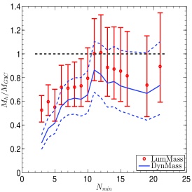
The G³Cv5 catalogue comes with two mass estimates. A typical usage of these estimates involves investigating other group properties at fixed group mass (e.g., Guo et al., 2014; Oliva-Altamirano et al., 2014). In this section we compare the weak lensing measured masses within these bins with the G³Cv5 estimates. To this end, we measure the ratio of halo mass to G³Cv5 mass within each bin, and also try a power-law fit to the relation between the ratio and the G³Cv5 mass, i.e. $M_{h}/M_{G3C}=A(M_{G3C}/10^{14}h^{-1}\mathrm{M}_{\odot})^{\alpha}$. The results are shown in the left and middle panels of Fig. 10. In general, the WL-measured masses are smaller than the G³Cv5 masses. At their closest, for haloes around $10^{13}-10^{14}h^{-1}\mathrm{M}_{\odot}$, the G³Cv5 mass estimates are still larger than the WL ones by $0.1-0.2$ dex. The global power-law fit to the dynamical mass bias yields $\log(A)=-0.54-0.22\pm 0.10$ and $\alpha=-0.31+0.04\pm 0.15$. The fit to the luminosity mass bias gives a slope that is consistent with zero, so we fix it to be zero and find $\log(A)=-0.28-0.09\pm 0.09$. This means that the weak lensing mass measurement is $3.5$ times smaller than the dynamical mass estimates near $10^{14}h^{-1}\mathrm{M}_{\odot}$, or $\sim 2$ times smaller than the luminosity mass globally. Similar biases are observed in the mock catalogues when comparing the input halo masses with those from the G³Cv5 mass estimators. The slope for the dynamical mass bias in the mocks is somewhat steeper than that shown by the groups in the G³Cv5 itself, reflecting the different mass-velocity dispersion relation that we observed in Section 5.2. The agreement between luminosity mass and lensing mass is slightly better, although the discrepancy is amplified when systematic corrections are taken into account.

Figure 10: Left and middle panels: the biases of halo mass with respect to the G³Cv5 mass estimates, where G³Cv5 mass refers to dynamical (left) and luminosity (middle) mass in the two panels. In both cases, the red data points are the MLWL measured mass ratio within each G³Cv5 mass bin; the black solid line is a power-law MLWL fit to the mass ratio-G³Cv5 mass relation in the whole sample; the black dashed line is the fit with systematic corrections; the green solid lines are the median relations in the nine mock catalogues, while the green dashed lines mark the typical 16th and 84th (i.e., $\pm 1\sigma$) percentiles in one mock. Note that for luminosity mass the power-law fit gives a slope so close to zero that we have fixed it to be zero. Right panel: The measured bias of the G³Cv5 mass estimates adopting different multiplicity cuts $N_{\rm min}$. The red points with error bars show the bias of the G³Cv5 luminosity mass. The blue solid line is the measured bias of the G³Cv5 dynamical mass, and the blue dashed lines are the error bounds.

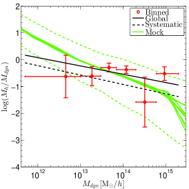
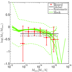
The presence of bias at fixed estimated mass does not conflict with the G³Cv5 claim of a global median unbiased mass calibration. The G³Cv5 calibration is done ensuring that the estimated masses are unbiased with respect to the real group masses in their global median value. Also, only the dynamical mass is calibrated with halo masses in the mock. The luminosity mass is subsequently calibrated against the dynamical mass. While Robotham et al. (2011) split the G³Cv5 groups into multiplicity and redshift bins, they did not find unbiased mass estimates for each dynamical or luminosity mass bin. This calibration thus leaves room for a mass-dependent bias both below and above the median mass value. The problem can become more severe if the mass-velocity dispersion-radius relation, which is used as a primary mass estimator, differs between the data and the mock. Unfortunately, such a difference is just what we have observed using our lensing measurement–a conclusion that can only be reached using an independent mass measurement such as lensing. Finally, the G³Cv5 calibration is only done using FoF groups that are bijectively matched with particular haloes. As a result, an overall bias could also show up when one examines the masses of the entire group sample. These three effects combined result in both an overall and a mass-dependent bias of our mass measurement with respect to the G³Cv5 estimates. This bias also propagates to the G³Cv5 luminosity mass, which is a secondary estimator.

The G³Cv5 masses become less biased with higher multiplicity cuts. In the right panel of Figure 10, we show the measured bias of the G³Cv5 dynamical and luminosity masses when adopting different multiplicity cuts $N\geq N_{\rm min}$. With higher multiplicity cuts, the biases become weaker, and are consistent with unity for $N>10$ groups.

6.2 Constructing Mass Estimators

Figure 11: The performance of different mass estimators applied to the mock catalogue for groups with $N\geq 3$. In each panel, the contour lines mark the 30th, 60th and 90th percentiles of the 2D density distribution. The red solid line is the median distribution of actual halo mass, conditioned on observed mass, with red dashed lines showing the 16th and 84th (i.e., $\pm 1\sigma$) percentiles. The top panels are for the G³Cv5 estimators as calibrated in Robotham et al. (2011), while the others show our new estimators from Table 1. Note that systematic corrections have been applied to the parameters.

Figure 12: Same as Fig. 11 but for $N\geq 2$ groups.

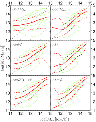
To allow a more general parametrization of the dynamical mass, we consider power-law combinations of six physical observables: $V_{N}$, $(1+z)$, $\sigma_{v}$, $R_{50}$, $L_{\rm grp}$ of the groups and $M_{\star}$ of group central galaxies. While we have considered simultaneous independent variations of all of the six power-law exponents, appropriate subsets of these variables, with all other exponents fixed to zero, are able to provide a good mass estimator.

According to Equation (22), the model with the highest $TS$ would also be the one with the least scatter, $\sum_{i}(\frac{\Delta S_{i}}{N_{i}})^{2}$. In other words, for a given sample, $TS$ is a measurement of the intrinsic tightness of each mass-observable relation. To account for both the improvement in fit and the number of degrees of freedom in the model, the lowest $p$-value (or highest significance) combination of these parameters is found. With a significance of $7.23\sigma$ derived from $TS$ relative to a null model with no lensing mass present, the best choice is of the form

$$M\propto L_{\rm grp}^{\alpha_{L}}\sigma_{v}^{\alpha_{\sigma}}(1+z)^{\alpha_{z}}.$$ (34)

The best-fit parameters are listed in Table 1.

Since the $TS$ value can be diluted in the presence of systematics, we also tried the above selection process with $TS^{\prime}=TS/b$. As listed in Table 1, the estimated $b$ is $\sim 2-5$, and is primarily set by the systematic uncertainty in the mass dispersion, $\sigma_{\log M}$. Given the uncertainty in how well the modelled mass dispersion mimics that in the real data, it is unclear which of $TS$ or $TS^{\prime}$ provides a better measure of significance. Hence we consider both in an effort to provide insight into the robustness of the results. If we assume a common value of $b$ for all estimators, then for $b$ in the range $2-20$, the best construction is simply

$$M\propto L_{\rm grp}^{\alpha_{L}}.$$ (35)

The significance according to the raw $TS$ is $7.0\sigma$.

Simple combinations of $V_{N}$ with $\sigma_{v}$ or $L_{\rm grp}$ can achieve comparable significance to the best combinations given above, in the forms

$$M\propto\sigma_{v}^{\alpha_{\sigma}}V_{N}^{\alpha_{V}}$$ (36)

and

$$M\propto L_{\rm grp}^{\alpha_{L}}V_{N}^{\alpha_{V}}.$$ (37)

Note that $V_{N}\propto L_{\rm grp}$ if we assume a universal luminosity function for both group and field galaxies. Consequently, the estimator $M(V_{N},\sigma,z)$ has a comparable significance to $M(L_{\rm grp},\sigma,z)$. In addition, estimators that explicitly depend on $L_{\rm grp}$ and $z$ are expected to be robust to changes in the survey selection function described by $V_{N}^{\rm lim}(z)$. Again the best-fit parameters for all the above estimators can be found in Table 1.

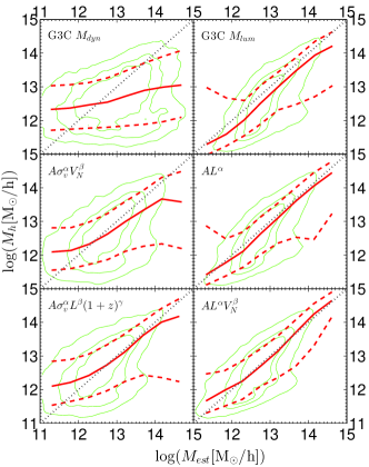
In Fig. 11 we show the joint distributions of true mass in the mocks, for $N\geq 3$ groups, and estimated mass derived from our mass estimators, calibrated with real lensing measurements, as well as the G³Cv5 mass estimators with their official calibration. The G³Cv5 dynamical mass estimator has both the largest bias and scatter. As shown in Section 6.1, the G³Cv5 luminosity mass estimator is also biased, despite having been carefully tuned at different multiplicities and redshifts. Combining velocity dispersion with $V_{N}$ instead of $R_{50}$ results in a much improved dynamical estimator. The performance can be further improved when $\sigma_{v}$ is combined with $L_{\rm grp}$ and $z$, but the estimation of $L_{\rm grp}$ from observed group properties does involve many more steps than is the case for $V_{N}$. Bravely applying our $N\geq 3$ calibrated estimators to $N\geq 2$ groups in the mock still produces good results for all the new estimators except $M(\sigma,V_{N})$, as seen in Fig. 12.

We caution that the performance of different estimators in the mocks should not be taken as conclusive, since the mocks may not be an appropriate realization of the real universe. In particular, haloes below $10^{12}h^{-1}\mathrm{M}_{\odot}$ are resolved by at most $\sim 1000$ particles in the Millennium simulation. In this mass range, fewer than $100$ particles will typically lie within subhaloes in any given halo, and any galaxies associated with these subhaloes will be less numerically reliable than one might wish. Hence one expects that the mock catalogue will provide a deficient representation for haloes below $10^{12}h^{-1}\mathrm{M}_{\odot}$.

7 Conclusions

We have carried out a maximum-likelihood weak lensing analysis on a set of SDSS source galaxies located in the GAMA survey regions, in order to derive halo masses for the GAMA galaxy groups. The group mass distribution is modelled with an NFW profile, with a mass-concentration relation fixed by previous simulation results. This enables us to predict the gravitational shear produced by each halo with a single parameter, namely halo mass. Comparing the predicted shear with the observed shapes of background galaxies allows us to fit the halo mass of our foreground lenses. By splitting the G³Cv5 group sample according to various observed properties, we have explored the scaling relations between halo mass and these observables. With power-law parametrization of these relations, global fits over the entire sample are also performed. The resulting likelihood ratios quantify the intrinsic tightness of each mass-observable relation. All the fitted results are summarized in Table 1. The dominant systematic uncertainty in our measured mass-observable relations comes from the assumed halo mass dispersion around the median, modelled as a lognormal distribution in mass.

We emphasize that the majority of our measurements are based on the multiplicity-limited G³Cv5 group sample, and are subject to the group selection function described by $V_{N}\leq V_{N}^{\rm lim}(z)$. The only exception is the measured halo mass-stellar mass relation where a volume-limited stellar mass sample is specially constructed. Proper comparison of our results with theory or other measurements have to take the selection effect into account. To help interpret our results and to compare with theoretical predictions we have constructed mock catalogues based on the application of the GALFORM semianalytic model of galaxy formation (Bower et al., 2006) to halo merger trees in the $\Lambda$CDM Millennium N-body simulation Springel et al. (2005). The mock catalogues are generated using the selection function of the real GAMA survey. For the first time, identifical group finding algorithms and selection functions have been applied to both observational data and lightcone galaxy mocks to enable side-by-side comparisons between lensing measurements and a semi-analytic model. Overall there is very good agreement between our measured mass-observable relations and those predicted by the galaxy formation model. In particular, we find that:

• The halo mass scales roughly in proportion to group luminosity, multiplicity volume and central galaxy stellar mass in the multiplicity limited G³Cv5 sample. These relations are in excellent agreement with predictions from the mocks.

• For given stellar mass of the central galaxy, the halo mass strongly depends on the number of galaxies in the group. To compare our measurement with existing HOD models, we have constructed a volume limited central galaxy catalogue, and measured the stellar mass-halo mass relation free from selection effects. We find the measurement of the $M_{h}(M_{\star})$ relation provides a very powerful constraint on the HOD scatter of the $M_{\star}(M_{h})$ relations. A dispersion $\sigma_{\log(M_{\star})}=0.2$, or $0.15$ after subtracting the stellar mass measurement noise, is able to yield a good agreement between our measurement and all the HOD predictions that we considered.

• The measured $M_{h}(\sigma_{v})$ relation shows a slightly different slope from that in the mocks, which could originate from the velocity bias of galaxies with respect to dark matter. The measured $M_{h}(R_{50})$ relation is also in slight tension with those in the mock catalogues at small $R_{50}$. Such a small scale discrepancy is also obvious in the $L_{\rm grp}(R_{50})$ scaling of groups. It can be partly explained by the limited spatial resolution of the Millennium simulation, and may also reflect the treatment of orphan galaxies in the model.

• The G³Cv5 mass estimators are biased when used for stacking. Luminosity mass has a small but constant bias, while dynamical mass can have a large and mass-dependent bias. A globally calibrated mass-to-light relation can serve as a very good mass estimator for groups, and is the tightest halo mass to single observable relation in our sample. The estimation can be slightly improved when combined with $V_{N}$. The mass estimates from dynamical measurements can be much improved when combining $\sigma_{v}$ with $V_{N}$ instead of $R_{50}$, or when combined with group luminosity and redshift.

• The dominant source of systematic uncertainty in our mass estimators comes from the assumed dispersion in halo mass about the median value, modelled with a lognormal distribution in mass. For a mass dispersion of $0.5-0.7$ dex, the resulting overestimation in median lens mass is typically $0.2-0.3$ dex. This is slightly counteracted by smaller underestimations caused by uncertainties in the redshifts of background photometric galaxies and the positions of gravitational centres of foreground lenses. Selection cuts in the data do not cause significant biases in the results. The systematic uncertainties considered here change the slopes of the mass-observable relations by only $0.01$, but do have a greater impact on the significance of the results, reducing $TS$ for the fits by a factor of $2-5$.

In this work we have taken a galaxy-by-galaxy maximum-likelihood approach to extract the lensing signal of galaxy groups. Compared with stacked weak lensing, our approach makes much more efficient use of the information contained in individual galaxy shapes. In addition, our utilization of the information carried by individual lenses is also more efficient, since our fitting can be done free from binning. In contrast, stacked weak lensing usually measures a weighted average density profile of the underlying, to be modelled, matter distribution. This involves averaging over the distribution of halo masses and redshift. A direct fitting without knowing the underlying sample distribution and the stacking weights leaves the result difficult to interpret, or gives biased results if bravely interpreted as the average mass of the sample. A further complication in stacked lensing comes from the redshift evolution of halo profiles. Haloes evolve with redshift, as do the definitions of the halo mass and edge, so the same halo mass does not correspond to the same profile in either physical or comoving coordinates. It is not clear what is the best coordinate system for stacking. In contrast, our likelihood fitting deals with each halo separately, and can properly incorporate any distribution and evolution in halo density profiles. We note that stacked lensing could complement MLWL by providing a non-parametric measurement of the average density profile. In this work we only do stacked weak lensing for visualization of the measured and fitted profiles.

We plan to explore the mass-concentration relation and the halo mass function probed by GAMA in subsequent papers. This methodology would also be well suited for higher redshift, using the combination of the VIPERS survey (Guzzo et al., 2013), which has 100,000 spectroscopic galaxies with $0.5<z<1.2$, and the CFHTLens source catalogue, which has a median redshift $\sim 0.75$ and a source density of $17~{}\rm{arcmin}^{-2}$. The KiDS survey (de Jong et al., 2013) has just come to its first data release of $50$ square degree data overlapping with GAMA. Adopting the KiDS shear catalogue, we expect to have more than a factor of 3 improvement in signal to noise ratio.

Appendix A Ellipticity measurements

The shapes of the source galaxies in this work are measured using the re-Gaussianisation technique by Mandelbaum et al. (2005a); Reyes et al. (2012), which we briefly describe here. The convolution of a galaxy image with a point spread function (PSF) has two major effects that we seek to remove. Firstly, since the PSF is generally close to round, it circularises the apparent galaxy shape; this is known as PSF dilution, and the correction for it can be a factor of $\sim 2$ for typical-sized galaxies. Secondly, since the PSF has some small ellipticity (the PSF anisotropy), that ellipticity is imprinted coherently into the shapes of all galaxies. If uncorrected then this gives rise to a coherent additive systematic error in galaxy shapes and inferred lensing shears. The goal of a PSF correction method is to allow one to infer galaxy shapes by correcting for both of these effects, and thereby infer the lensing shear.

Historically, the earliest methods of PSF correction were based on correcting the second moments of the observed galaxy image using the second moments of the PSF to derive the correction factor (e.g., Kaiser et al. 1995). The method that we use here, re-Gaussianization, is a moments-based technique that corrects for non-Gaussianity of the PSF (provided that it is small, as for ground-based PSFs) and for kurtosis of the galaxy profile. In brief, the correction proceeds in two steps. In the first step, the PSF is split into a Gaussian image, $G(x)$, plus a residual, $\epsilon(x)$, so that the observed image can be written as

$$I=(G+\epsilon)\otimes f=G\otimes f+\epsilon\otimes f,$$ (38)

where $f$ is the pre-seeing galaxy profile, and all quantities are implicitly functions of position (but we have suppressed the argument). We make a simple elliptical Gaussian approximation, $f^{\prime}$ to $f$, and use that to derive a new image $I^{\prime}$ defined as

$$I^{\prime}=I-\epsilon\otimes f^{\prime}\simeq G\otimes f.$$ (39)

While our approximation to $f$ is a simple one, we rely on the fact that the residual from a Gaussian PSF ($\epsilon$) is quite small. Our new image, $I^{\prime}$, can be interpreted as an image of what the galaxy would have looked like if it had been convolved with a simple Gaussian PSF. We can therefore carry out the second step of our PSF correction process using a moments-based method that corrects for the lowest order of non-Gaussianity in the galaxy profiles, but assumes a Gaussian PSF (Bernstein & Jarvis, 2002) in order to estimate a per-object galaxy ellipticity. For more details on this entire process, see Hirata & Seljak (2003). The re-Gaussianization method has been tested extensively on real and simulated data (Mandelbaum et al., 2005a; Reyes et al., 2012; Mandelbaum et al., 2012, 2013) with calibration that is well-controlled at the percent level.

Appendix B Further discussion of systematics

We expand in this section several discussions on systematics related to various datacuts introduced in Section 4.1. These include our choice of the redshift cut, the influence of unmodelled lenses mentioned in the virial cut and in Section 4.2, and the effect of the multiplicity cut, which was discussed in Sections 5.3 and 5.4.

B.1 Suppressing foreground contamination

To quantify the amount of contamination in the source sample from foreground group member galaxies, we extract the correlation function of background galaxies with foreground lenses. Specifically, we count the average number density, $n$, of background galaxies around foreground lenses, and compare them with the average number density of random galaxies around lenses, $n_{\rm rand}$. The random galaxies are generated by randomizing the position of background galaxies inside the survey region, so that the random sample will have the same size and follow the same redshift distribution as the real sample. The contamination level, or the lens-source correlation function, can then be estimated from $\xi=n/n_{\rm rand}-1$. In Fig. 13 we show the estimated correlation for our adopted minimum redshift separation of $\Delta z=0.3$, around different mass haloes. For comparison, the correlation for the most massive bin with $\Delta z=0.01$ is also shown. While it is obvious that the contamination is large with a small $\Delta z$, it can be mostly eliminated with our redshift cut.

Figure 13: Contamination in the background source sample from foreground galaxies, for lenses in three luminosity mass bins. The L1, L2 and L3 bins have mean mass $5\times 10^{12}$, $1.5\times 10^{13}$ and $8\times 10^{13}h^{-1}\mathrm{M}_{\odot}$, and mean redshifts of $0.12$, $0.18$ and $0.25$, and a minimum redshift separation of $\Delta z=0.3$. For comparison we also show the L3 bin with $\Delta z=0.01$ (L3Tight). Error-bars mark the $2\sigma$ uncertainty estimated from 1000 mock samples.

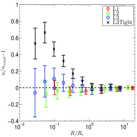
B.2 Influence of the two halo term

We have ignored the contribution of the two halo term (see, e.g. Mandelbaum et al., 2005b; Johnston et al., 2007; Hayashi & White, 2008) on large scales throughout this paper. Since this term arises from the correlated distribution of haloes, the missing contribution comes from unmodelled haloes. By adding a two halo term to the mass model in our Monte Carlo shear map simulation, and fitting the simulated map with our standard procedure, we have estimated that the bias introduced by completely missing the two halo term is a $\sim 3$ per cent overestimate in mass.Since this procedure double-counts the two-halo term if we include it for every halo at every separation, the influence from the two-halo term is already overestimated. Hence we ignore it throughout this paper.

B.3 Absolute multiplicity dependence of the mass-observable relations

The group selection function of our current catalogue is described by the multiplicity volume $V_{N}$ (see Equation 30 and 31), or equivalently the absolute multiplicity. To understand better how this selection function affects our measurements of mass-observable relations, in this section we explore explicitly the dependence of these relations on the absolute multiplicity. We have selected, from the Bower et al. (2006) model in the Millennium database, two samples of haloes within a narrow range of either luminosity or central galaxy stellar mass. In Fig. 14, We plot the halo mass of these objects as a function of their luminosity or central stellar mass, and color-code them with absolute multiplicity. Here the absolute multiplicity $N_{\rm abs}$ is defined to be the number of galaxies in the halo with an absolute $r$-band magnitude $r<-13$. The scatter of these mass observable relations at fixed observable value is clearly not stochastic, but correlates strongly with $N_{\rm abs}$. As a result, the measured mass-observable relations in a multiplicity-limited group sample will generally be higher than those in a volume-limited sample, since groups with lower absolute multiplicities are more likely to be missing in the sample, consistent with what we see in Fig. 7 of Section 5.4.

Figure 14: The role of group absolute multiplicity in the mass-observable relations. In the left panel, we plot the halo mass-luminosity relation for all haloes with $10^{11}h^{-2}\mathrm{L}_{\odot}<L_{\rm grp}<2\times 10^{11}h^{-2}\mathrm{L}_{\odot}$, colour-coded by $N_{\rm abs}$. The right panel is similar but for the halo mass-central galaxy stellar mass relation of systems with central galaxy stellar masses in the range $9\times 10^{10}h^{-2}\mathrm{M}_{\odot}<M_{\star}<10^{11}h^{-2}\mathrm{M}_{\odot}$.

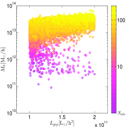
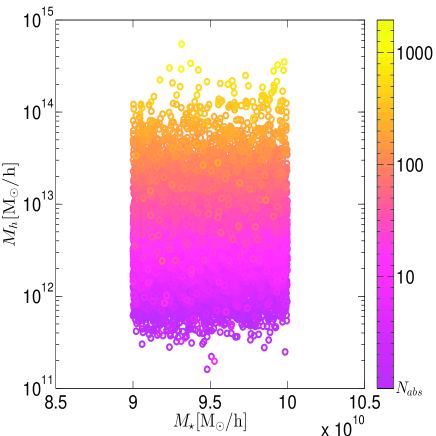
Appendix C Stellar mass-halo mass relations

We convert the fitted average central galaxy stellar mass-halo mass relations in the literature to the following form where possible, and list the parameters in Table 2, along with their adopted HOD dispersion:

$$M_{\star}=\frac{AM_{h}}{\left[\left(\frac{M_{h}}{M_{0}}\right)^{\alpha}+\left(\frac{M_{h}}{M_{0}}\right)^{\beta}\right]^{\gamma}}.$$ (40)

The halo mass $M_{h}$ is defined to have an average density of 200 times the background matter density. This functional form, especially with $\gamma=1$ as in Yang et al. (2003), or similar functions to represent two power-laws with a smooth transition, has been frequently used to fit the observed galaxy stellar mass distribution to a modelled halo mass distribution (e.g. Wang et al., 2006; Yang et al., 2008; Wang & Jing, 2010; Moster et al., 2010, 2013; Guo et al., 2010; Behroozi et al., 2010, 2013; Wang et al., 2013b). The different relations largely agree at the low mass end, where there are good constraints, and differ significantly at the high mass end. All the listed relations adopt a Chabrier IMF. These relations are compared with our measurements in Section 5.4.

Table 2: HOD model parameters for the central galaxy stellar mass-halo mass distribution, with the average relation of the form given by Equation (40), and halo mass defined to have an average density of $200$ times the background matter density. The final column lists the assumed dispersion in the stellar mass at fixed halo mass.

Model	$A$	$\log(M_{0}/h^{-1}\mathrm{M}_{\odot})$	$\alpha$	$\beta$	$\gamma$	$\sigma_{\log(M_{\star})}$
WangL13 (Wang et al., 2013a)	0.0387	11.67	-1.56	0.66	1	0.17
WangLY13 (Wang et al., 2013b)	0.0372	11.70	-1.16	0.71	1	0.22
Moster13 (Moster et al., 2013)	0.0370	11.58	-1.38	0.61	1	0.1
Guo10 (Guo et al., 2010)	0.0690	11.40	-0.926	0.261	2.44	0

Appendix D Stacked group density profiles

As a sanity check, in this section we show the stacked density profiles of our group sample, and compare them with the predictions from our MLWL fits.

Following Mandelbaum et al. (2006a), we adopt the following estimator for the average comoving surface overdensity profile around haloes of similar mass stacked in comoving cooordinates:

$$\langle\Delta\Sigma(r)_{\rm cmv}\rangle=\frac{\sum_{i}{w_{i}\chi_{t,i}\Sigma_{\rm crit,i}a^{2}_{\ell,i}}}{2\mathscr{R}\sum_{i}{w_{i}}}.$$ (41)

Here, $\Sigma_{\rm cmv}(r)=\bar{\rho}\int_{l.o.s}\delta_{m,{\rm cmv}}(r)dl$ is the comoving overdensity of matter integrated along the line of sight, and $\langle\Delta\Sigma_{\rm cmv}(r)\rangle=\langle\Sigma_{\rm cmv}(<r)\rangle-\langle\Sigma_{\rm cmv}(r)\rangle$ is the difference between the average surface overdensity within a radius $r$ and that at $r$. The subscript $i$ runs over all the lens-source pairs in the sample. $a_{\ell}$ is the scale factor at the lens redshift, $\chi_{t}$ is the tangential ellipticity of the source galaxy with respect to the lens, and the weighting function is chosen to be

$$w_{i}=\frac{1}{(\Sigma_{\rm crit,i}a^{2})^{2}(\sigma_{\chi_{i}}^{2}+\sigma_{SN}^{2})}.$$ (42)

With this weighting scheme, the responsivity is calculated using (Bernstein & Jarvis, 2002)

$$\mathscr{R}=\frac{\sum_{i}{w_{i}[1-(1-f_{i})\sigma_{SN}^{2}-{f_{i}^{2}\chi_{i}^{2}}/{2}}]}{\sum_{i}{w_{i}}},$$ (43)

where $f_{i}={\sigma_{SN}^{2}}/({\sigma_{SN}^{2}+\sigma_{\chi_{i}}^{2}})$. The responsivity is almost independent of radius.

Ignoring the error on shear responsivity, the covariance of the estimated surface density at radii $r_{I}$ and $r_{J}$ can be written as

$$C(\Delta\Sigma_{I},\Delta\Sigma_{J})=\\ \frac{\sum_{i\in I,j\in J}{w_{i}\Sigma_{\rm crit,i}a^{2}_{\ell,i}}{w_{j}\Sigma_{\rm crit,j}a^{2}_{\ell,j}}C(\chi_{t,i},\chi_{t,j})}{4\mathscr{R}^{2}\sum_{i\in I}{w_{i}}\sum_{j\in J}{w_{j}}}.$$ (44)

Suppose the ellipticities of different galaxies are independent, then correlations of tangential ellipticity only exist if the two lens-source pairs are constructed from the same source galaxy, i.e.

$$\mathrm{C}(\chi_{t,i},\chi_{t,j})=\\ \left\{\begin{array}[]{rl}\cos(2\phi_{ij})(\sigma_{SN}^{2}+\sigma_{\chi_{i}}^{2})&\mbox{common source galaxy}\\ 0&\mbox{ otherwise,}\end{array}\right.$$ (45)

where $\phi_{ij}$ is the angle subtended by lens-source pair $ij$. The equations above fully account for the correlated error introduced by multiple use of the same source galaxy in the stacking. These estimated errors give consistent results with chunked bootstrap measurements. Jeong & Komatsu (2009) have also derived a continuous version of the covariance matrix for stacked lensing that accounts for cosmic variance.

Figure 15: Stacked surface density profile for all the groups used in this work. Points with errorbars are the stacked profiles. Different lines are the predicted surface density profiles from various mass estimates, stacked exactly the same way as for the data. As labelled in the figure, the dynamical and luminosity masses are the standard G³Cv5 calibrated mass estimators, while other lines are power-law combinations of the listed observables.

Figure 16: Stacked surface density profile for groups with different luminosities. From left to right, groups are selected by luminosities in the range of $(0.1-1)\times 10^{11}h^{-2}\mathrm{L}_{\odot}$, $(1-5)\times 10^{11}h^{-2}\mathrm{L}_{\odot}$ and $(5-50)\times 10^{11}h^{-2}\mathrm{L}_{\odot}$. Line styles are the same as in Fig. 15. Note that no radial cut has been applied in producing this plot.

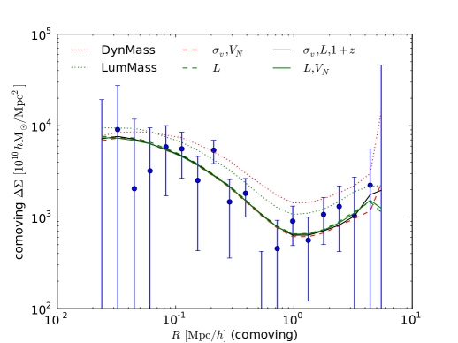
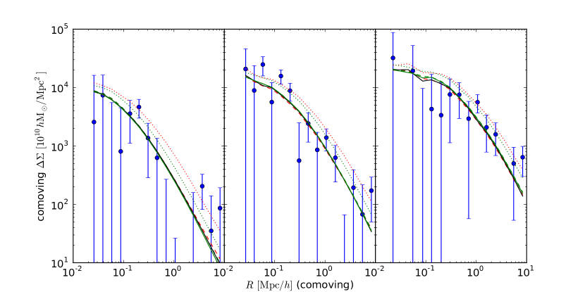
Fig. 15 shows the stacked surface density profile of groups, with the same data cuts as applied in the likelihood analysis. Since we have halo mass estimates for each individual group from Section 6.2, we can stack the inferred projected NFW profiles in exactly the same way as we stack the data. This gives predicted stacked profiles that are directly comparable with the measured profiles, free from any averaging ambiguities, under the assumption that the predicted mass is taken as the real mass of each group. No systematic corrections are applied in the mass estimates during stacking, to make a fair comparison with the measured profiles for which no correction is made either. It can be seen that our newly calibrated mass estimators lead to model stacked profiles that agree very well with each other, as well as with the measurement, while the G³Cv5 estimates overpredict the measured profile. The rise in the profile at large radius is caused by our virial cut, $R<2R_{200b}$, for each group, which implies that the smaller haloes cannot contribute at large radii and are hence unable to dilute the average stacked surface density profile here.

In Fig. 16, we show the stacked surface density profiles split into three luminosity bins. This time no radial cut is applied. The measured and modelled profiles are in good agreement in all cases. Good agreement is also observed between the data and our estimators.

References

- Adachi & Kasai (2012) Adachi M., Kasai M., 2012, Progress of Theoretical Physics, 127, 145, arXiv:1111.6396
- Adelman-McCarthy et al. (2008) Adelman-McCarthy J. K. et al., 2008, ApJS, 175, 297, arXiv:0707.3413
- Bartelmann & Schneider (2001) Bartelmann M., Schneider P., 2001, Phys. Rep., 340, 291, astro-ph/9912508
- Beers et al. (1990) Beers T. C., Flynn K., Gebhardt K., 1990, AJ, 100, 32
- Behroozi et al. (2010) Behroozi P. S., Conroy C., Wechsler R. H., 2010, ApJ, 717, 379, arXiv:1001.0015
- Behroozi et al. (2013) Behroozi P. S., Wechsler R. H., Conroy C., 2013, ApJ, 770, 57, arXiv:1207.6105
- Bernstein & Jarvis (2002) Bernstein G. M., Jarvis M., 2002, AJ, 123, 583, astro-ph/0107431
- Blanton et al. (2003) Blanton M. R. et al., 2003, ApJ, 592, 819, astro-ph/0210215
- Bower et al. (2006) Bower R. G., Benson A. J., Malbon R., Helly J. C., Frenk C. S., Baugh C. M., Cole S., Lacey C. G., 2006, MNRAS, 370, 645, astro-ph/0511338
- Brown et al. (2008) Brown M. J. I. et al., 2008, ApJ, 682, 937, arXiv:0804.2293
- Budzynski et al. (2012) Budzynski J. M., Koposov S. E., McCarthy I. G., McGee S. L., Belokurov V., 2012, MNRAS, 423, 104, arXiv:1201.5491
- Choi et al. (2012) Choi A., Tyson J. A., Morrison C. B., Jee M. J., Schmidt S. J., Margoniner V. E., Wittman D. M., 2012, ApJ, 759, 101, arXiv:1208.3904
- Colless et al. (2001) Colless M. et al., 2001, MNRAS, 328, 1039, astro-ph/0106498
- Cooray & Sheth (2002) Cooray A., Sheth R., 2002, Phys. Rep., 372, 1, astro-ph/0206508
- de Jong et al. (2013) de Jong J. T. A., Verdoes Kleijn G. A., Kuijken K. H., Valentijn E. A., 2013, Experimental Astronomy, 35, 25, arXiv:1206.1254
- Driver et al. (2011) Driver S. P. et al., 2011, MNRAS, 413, 971, arXiv:1009.0614
- Duffy et al. (2008) Duffy A. R., Schaye J., Kay S. T., Dalla Vecchia C., 2008, MNRAS, 390, L64, arXiv:0804.2486
- Eke et al. (2004a) Eke V. R. et al., 2004a, MNRAS, 348, 866, astro-ph/0402567
- Eke et al. (2004b) Eke V. R. et al., 2004b, MNRAS, 355, 769, astro-ph/0402566
- Farrow (2013) Farrow D., 2013, PhD thesis, Durham University
- Feldmann et al. (2006) Feldmann R. et al., 2006, MNRAS, 372, 565, astro-ph/0609044
- George et al. (2012) George M. R. et al., 2012, ApJ, 757, 2, arXiv:1205.4262
- Giocoli et al. (2010) Giocoli C., Tormen G., Sheth R. K., van den Bosch F. C., 2010, MNRAS, 404, 502, arXiv:0911.0436
- Guo et al. (2013) Guo Q., Cole S., Eke V., Frenk C., Helly J., 2013, MNRAS, 434, 1838, arXiv:1301.3134
- Guo et al. (2014) Guo Q. et al., 2014, arXiv:1401.0986, arXiv:1401.0986
- Guo et al. (2010) Guo Q., White S., Li C., Boylan-Kolchin M., 2010, MNRAS, 404, 1111, arXiv:0909.4305
- Guzzo et al. (2013) Guzzo L. et al., 2013, arXiv:1303.2623, arXiv:1303.2623
- Han et al. (2012) Han J., Frenk C. S., Eke V. R., Gao L., White S. D. M., Boyarsky A., Malyshev D., Ruchayskiy O., 2012, MNRAS, 427, 1651, arXiv:1207.6749
- Hayashi & White (2008) Hayashi E., White S. D. M., 2008, MNRAS, 388, 2, arXiv:0709.3933
- Hilbert & White (2010) Hilbert S., White S. D. M., 2010, MNRAS, 404, 486, arXiv:0907.4371
- Hill et al. (2011) Hill D. T. et al., 2011, MNRAS, 412, 765, arXiv:1009.0615
- Hirata & Seljak (2003) Hirata C., Seljak U., 2003, MNRAS, 343, 459, astro-ph/0301054
- Hirata et al. (2004) Hirata C. M. et al., 2004, MNRAS, 353, 529, astro-ph/0403255
- Hoekstra et al. (2003) Hoekstra H., Franx M., Kuijken K., Carlberg R. G., Yee H. K. C., 2003, MNRAS, 340, 609, astro-ph/0211633
- Hoekstra et al. (2001) Hoekstra H. et al., 2001, ApJ, 548, L5, astro-ph/0012169
- Hoekstra et al. (2004) Hoekstra H., Yee H. K. C., Gladders M. D., 2004, ApJ, 606, 67, astro-ph/0306515
- Hudson et al. (2013) Hudson M. J. et al., 2013, arXiv:1310.6784, arXiv:1310.6784
- Hudson et al. (1998) Hudson M. J., Gwyn S. D. J., Dahle H., Kaiser N., 1998, ApJ, 503, 531, astro-ph/9711341
- James & Roos (1975) James F., Roos M., 1975, Comput.Phys.Commun., 10, 343
- Jeong & Komatsu (2009) Jeong D., Komatsu E., 2009, ApJ, 703, 1230, arXiv:0904.0497
- Jiang et al. (2008) Jiang C. Y., Jing Y. P., Faltenbacher A., Lin W. P., Li C., 2008, ApJ, 675, 1095, arXiv:0707.2628
- Jiang et al. (2013) Jiang L., Helly J. C., Cole S., Frenk C. S., 2013, arXiv:1311.6649, arXiv:1311.6649
- Johnston et al. (2007) Johnston D. E. et al., 2007, arXiv:0709.1159, arXiv:0709.1159
- Kaiser et al. (1995) Kaiser N., Squires G., Broadhurst T., 1995, ApJ, 449, 460, astro-ph/9411005
- Kelvin et al. (2012) Kelvin L. S. et al., 2012, MNRAS, 421, 1007, arXiv:1112.1956
- Kilbinger et al. (2013) Kilbinger M. et al., 2013, MNRAS, 430, 2200, arXiv:1212.3338
- Kravtsov et al. (2014) Kravtsov A., Vikhlinin A., Meshscheryakov A., 2014, arXiv:1401.7329, arXiv:1401.7329
- Leauthaud et al. (2012) Leauthaud A. et al., 2012, ApJ, 744, 159, arXiv:1104.0928
- Li et al. (2012) Li C., Jing Y. P., Mao S., Han J., Peng Q., Yang X., Mo H. J., van den Bosch F., 2012, ApJ, 758, 50, arXiv:1206.3566
- Lin & Mohr (2004) Lin Y.-T., Mohr J. J., 2004, ApJ, 617, 879, astro-ph/0408557
- Lin et al. (2004) Lin Y.-T., Mohr J. J., Stanford S. A., 2004, ApJ, 610, 745, astro-ph/0402308
- Loveday et al. (2012) Loveday J. et al., 2012, MNRAS, 420, 1239, arXiv:1111.0166
- Mandelbaum et al. (2012) Mandelbaum R., Hirata C. M., Leauthaud A., Massey R. J., Rhodes J., 2012, MNRAS, 420, 1518, arXiv:1107.4629
- Mandelbaum et al. (2005a) Mandelbaum R. et al., 2005a, MNRAS, 361, 1287, astro-ph/0501201
- Mandelbaum et al. (2010) Mandelbaum R., Seljak U., Baldauf T., Smith R. E., 2010, MNRAS, 405, 2078, arXiv:0911.4972
- Mandelbaum et al. (2006a) Mandelbaum R., Seljak U., Cool R. J., Blanton M., Hirata C. M., Brinkmann J., 2006a, MNRAS, 372, 758, astro-ph/0605476
- Mandelbaum et al. (2006b) Mandelbaum R., Seljak U., Kauffmann G., Hirata C. M., Brinkmann J., 2006b, MNRAS, 368, 715, astro-ph/0511164
- Mandelbaum et al. (2013) Mandelbaum R., Slosar A., Baldauf T., Seljak U., Hirata C. M., Nakajima R., Reyes R., Smith R. E., 2013, MNRAS, 432, 1544, arXiv:1207.1120
- Mandelbaum et al. (2005b) Mandelbaum R., Tasitsiomi A., Seljak U., Kravtsov A. V., Wechsler R. H., 2005b, MNRAS, 362, 1451, astro-ph/0410711
- Marian et al. (2010) Marian L., Smith R. E., Bernstein G. M., 2010, ApJ, 709, 286, arXiv:0912.0261
- Merson et al. (2013) Merson A. I. et al., 2013, MNRAS, 429, 556, arXiv:1206.4049
- Moster et al. (2013) Moster B. P., Naab T., White S. D. M., 2013, MNRAS, 428, 3121, arXiv:1205.5807
- Moster et al. (2010) Moster B. P., Somerville R. S., Maulbetsch C., van den Bosch F. C., Macciò A. V., Naab T., Oser L., 2010, ApJ, 710, 903, arXiv:0903.4682
- Munari et al. (2013) Munari E., Biviano A., Borgani S., Murante G., Fabjan D., 2013, MNRAS, 430, 2638, arXiv:1301.1682
- Murray et al. (2013) Murray S. G., Power C., Robotham A. S. G., 2013, Astronomy and Computing, 3, 23, arXiv:1306.6721
- Nakajima et al. (2012) Nakajima R., Mandelbaum R., Seljak U., Cohn J. D., Reyes R., Cool R., 2012, MNRAS, 420, 3240, arXiv:1107.1395
- Navarro et al. (1996) Navarro J. F., Frenk C. S., White S. D. M., 1996, ApJ, 462, 563, arXiv:astro-ph/9508025
- Navarro et al. (1997) Navarro J. F., Frenk C. S., White S. D. M., 1997, ApJ, 490, 493, arXiv:astro-ph/9611107
- Oliva-Altamirano et al. (2014) Oliva-Altamirano P. et al., 2014, MNRAS, 440, 762, arXiv:1402.4139
- Parker et al. (2005) Parker L. C., Hudson M. J., Carlberg R. G., Hoekstra H., 2005, ApJ, 634, 806, astro-ph/0508328
- Reddick et al. (2013) Reddick R. M., Wechsler R. H., Tinker J. L., Behroozi P. S., 2013, ApJ, 771, 30, arXiv:1207.2160
- Reyes et al. (2012) Reyes R., Mandelbaum R., Gunn J. E., Nakajima R., Seljak U., Hirata C. M., 2012, MNRAS, 425, 2610
- Robotham et al. (2011) Robotham A. S. G. et al., 2011, MNRAS, 416, 2640, arXiv:1106.1994
- Schneider et al. (2013) Schneider M. D. et al., 2013, MNRAS, 433, 2727, arXiv:1306.4963
- Schneider et al. (2012) Schneider M. D., Frenk C. S., Cole S., 2012, J. Cosmology Astropart. Phys, 5, 30, arXiv:1111.5616
- Schneider (2005) Schneider P., 2005, arXiv:astro-ph/0509252, astro-ph/0509252
- Schneider & Rix (1997) Schneider P., Rix H.-W., 1997, ApJ, 474, 25, astro-ph/9601190
- Sheldon et al. (2009) Sheldon E. S. et al., 2009, ApJ, 703, 2217, arXiv:0709.1153
- Sheth et al. (2001) Sheth R. K., Mo H. J., Tormen G., 2001, MNRAS, 323, 1, astro-ph/9907024
- Skibba et al. (2011) Skibba R. A., van den Bosch F. C., Yang X., More S., Mo H., Fontanot F., 2011, MNRAS, 410, 417, arXiv:1001.4533
- Springel et al. (2005) Springel V. et al., 2005, Nature, 435, 629, astro-ph/0504097
- Taylor et al. (2011) Taylor E. N. et al., 2011, MNRAS, 418, 1587, arXiv:1108.0635
- Tinker et al. (2008) Tinker J., Kravtsov A. V., Klypin A., Abazajian K., Warren M., Yepes G., Gottlöber S., Holz D. E., 2008, ApJ, 688, 709, arXiv:0803.2706
- Velander et al. (2013) Velander M. et al., 2013, arXiv:1304.4265, arXiv:1304.4265
- Wang et al. (2013a) Wang L., De Lucia G., Weinmann S. M., 2013a, MNRAS, 431, 600, arXiv:1211.4308
- Wang et al. (2013b) Wang L. et al., 2013b, MNRAS, 431, 648, arXiv:1203.5828
- Wang & Jing (2010) Wang L., Jing Y. P., 2010, MNRAS, 402, 1796, arXiv:0911.1864
- Wang et al. (2006) Wang L., Li C., Kauffmann G., De Lucia G., 2006, MNRAS, 371, 537, astro-ph/0603546
- Wang et al. (2014) Wang W., Sales L. V., Henriques B. M. B., White S. D. M., 2014, MNRAS, 442, 1363, arXiv:1403.2409
- Wilks (1938) Wilks S., 1938, Annals Math.Statist., 9, 60
- Wright & Brainerd (2000) Wright C. O., Brainerd T. G., 2000, ApJ, 534, 34
- Yang et al. (2003) Yang X., Mo H. J., van den Bosch F. C., 2003, MNRAS, 339, 1057, astro-ph/0207019
- Yang et al. (2008) Yang X., Mo H. J., van den Bosch F. C., 2008, ApJ, 676, 248, arXiv:0710.5096
- Yang et al. (2009) Yang X., Mo H. J., van den Bosch F. C., 2009, ApJ, 695, 900, arXiv:0808.0539
- Zheng et al. (2007) Zheng Z., Coil A. L., Zehavi I., 2007, ApJ, 667, 760, astro-ph/0703457
- Zitrin et al. (2012) Zitrin A., Bartelmann M., Umetsu K., Oguri M., Broadhurst T., 2012, MNRAS, 426, 2944, arXiv:1208.1766