Model-free quantification of time-series predictability
Abstract
This paper provides insight into when, why, and how forecast strategies fail when they are applied to complicated time series. We conjecture that the inherent complexity of real-world time-series data—which results from the dimension, nonlinearity, and non-stationarity of the generating process, as well as from measurement issues like noise, aggregation, and finite data length—is both empirically quantifiable and directly correlated with predictability. In particular, we argue that redundancy is an effective way to measure complexity and predictive structure in an experimental time series and that weighted permutation entropy is an effective way to estimate that redundancy. To validate these conjectures, we study 120 different time-series data sets. For each time series, we construct predictions using a wide variety of forecast models, then compare the accuracy of the predictions with the permutation entropy of that time series. We use the results to develop a model-free heuristic that can help practitioners recognize when a particular prediction method is not well matched to the task at hand: that is, when the time series has more predictive structure than that method can capture and exploit.
Keywords: entropy, permutation entropy, weighted permutation entropy, time-series analysis, predictability
pacs:
05.45.Tp 89.70.-a 89.75.Kd 95.75.PqI Introduction
Complicated time-series data are ubiquitous in modern scientific research. The complexity of these data spans a wide range. On the low end of this spectrum are time series that exhibit perfect predictive structure, i.e, signals whose future values can be successfully predicted from past values. Signals like this can be viewed as the product of an underlying process that generates information and/or transmits it from the past to the future in a perfectly predictable fashion. Constant or periodic signals, for example, fall in this class. On the opposite end of this spectrum are signals that are what one could call fully complex, where the underlying generating process transmits no information at all from the past to the future. White noise processes fall in this class. In fully complex signals, knowledge of the past gives no insight into the future, regardless of what model one chooses to use. Signals in the midrange of this spectrum, e.g., deterministic chaos, pose interesting challenges from a modeling perspective. In these signals, enough information is being transmitted from the past to the future that an ideal model—one that captures the generating process—can forecast the future behavior of the observed system with high accuracy.
This leads naturally to an important and challenging question: given a noisy real-valued time series from an unknown system, does there exist a forecast model that can leverage the information (if any) that is being transmitted forward in time by the underlying generating process? A first step in answering this question is to reliably quantify where on the complexity spectrum a given time series falls; a second step is to determine how complexity and predictability are related in these kinds of data sets. With these answers in hand, one can develop a practical strategy for assessing appropriateness of forecast methods for a given time series. If the forecast produced by a particular method is poor, for instance, but the time series contains a significant amount of predictive structure, one can reasonably conclude that that method is inadequate to the task and that one should seek another method. The goal of this paper is to develop effective heuristics to put that strategy into practice.
The information in an observation can be partitioned into two pieces: redundancy and entropy generation Crutchfield and Feldman (2003). Our approach exploits this decomposition in order to assess how much predictive structure is present in a signal—i.e., where it falls on the complexity spectrum mentioned above. We define complexity as a particular approximation of Kolmogorov-Sinai entropy Lind and Marcus (1995). That is, we view a random-walk time series (which exhibits high entropy) as purely complex, whereas a low-entropy periodic signal is on the low end of the complexity spectrum. This differs from the notion of complexity used by e.g. Shalizi and Crutchfield (2001), which would consider a time series without any statistical regularities to be non-complex. We argue that an extension of permutation entropy Bandt and Pompe (2002)—a method for approximating the entropy through ordinal analysis—is an effective way to assess the complexity of a given time series. Permutation entropy is ideal for our purposes because it works with real-valued data and is known to converge to the true entropy value. Other existing techniques either require specific knowledge of the generating process or produce biased values of the entropy Bollt et al. (2001).
We focus on real-valued, scalar, time-series data from physical experiments. We do not assume any knowledge of the generating process or its properties: whether it is linear, nonlinear, deterministic, stochastic, etc. To explore the relationship between complexity, predictive structure, and actual predictability, we generate forecasts for a variety of experimental time-series datasets using four different prediction methods, then compare the accuracy of those predictions to the permutation entropy of the associated signals. This results in two primary findings:
-
1.
The permutation entropy of a noisy real-valued time series from an unknown system is correlated with the accuracy of an appropriate predictor.
-
2.
The relationship between permutation entropy and prediction accuracy is a useful empirical heuristic for identifying mismatches between prediction models and time-series data.
There has, of course, been a great deal of good work on different ways to measure the complexity of data, and previous explorations have confirmed repeatedly that complexity is a challenge to prediction. It is well known that the way information is generated and processed internally by a system plays a critical role in the success of different forecasting methods—and in the choice of which method is appropriate for a given time series. This constellation of issues has not been properly explored, however, in the context of noisy, poorly sampled, real-world data from unknown systems. That exploration, and the development of strategies for putting its results into effective practice, is the primary contribution of this work. The empirical results in the later sections of this paper not only elucidate the relationship between complexity and predictability. The strategy that we derive from these results can also aid practitioners in choosing an appropriate prediction model for a given real-world noisy time series from an unknown system—a challenging task for which little guidance is currently available.
The rest of the paper is organized as follows. Section II discusses previous results on generating partitions, local modeling, and error distribution analysis, and situates this work in that context. Section III covers the experimental setup and methods used to collect the time-series data. Section IV describes the prediction models used in this study. Section V reviews permutation entropy, the technique that we use to measure complexity. In Section VI, we estimate the complexity of each empirical time series and compare that complexity to the accuracy of predictions produced by the methods of Section IV, operating on that time series. In Section VII, we discuss these results and their implications, and consider future areas of research.
II Related Work
Modeling time-series data for the purposes of prediction dates back at least to Yule’s 1927 invention of autoregression Yule (1927). Since then, hundreds, if not thousands, of strategies have been developed for a wide variety of prediction tasks. The purpose of this paper is not to add a new weapon to this arsenal, nor to do any sort of theoretical assessment or comparison of existing methods. Our goals are focused more on the practice of prediction: (i) to empirically quantify the predictive structure that is present in a real-valued scalar time series and (ii) to explore how the performance of prediction methods is related to that inherent complexity. It would, of course, be neither practical nor interesting to report results for every existing forecast method; instead, we choose a representative set, as described in Section IV.
Quantifying predictability, which is sometimes called “predicting predictability,” is not a new problem. Most of the corresponding solutions fall into two categories that we call model-based error analysis and model-free information analysis. The first class focuses on errors produced by a fixed forecasting schema. This analysis can proceed locally or globally. The local version approximates error distributions for different regions of a time-series model using local ensemble in-sample forecasting111The terms “in sample” and “out of sample” are used in different ways in the forecasting community. Here, we distinguish those terms by the part of the time series that is the focus of the prediction: the observed data for the former and the unknown future for the latter. In-sample forecasts—comparisons of predictions generated from part of the observed time series—are useful for assessing model error and prediction horizons, among other things.. These distributions are then used as estimates of out-of-sample forecast errors in those regions. For example, Smith et al. make in-sample forecasts using ensembles around selected points in order to predict the local predictability of that time series Smith (1992). This approach can be used to show that different portions of a time series exhibit varying levels of local predictive uncertainty. We expand on this idea later in this paper with a time series that exhibits interesting regime shifts.
Local model-based error analysis works quite well, but it only approximates the local predictive uncertainty in relation to a fixed model. It cannot quantify the inherent predictability of a time series and thus cannot be used to draw conclusions about predictive structure that may be usable by other forecast methods. Global model-based error analysis moves in this direction. It uses out-of-sample error distributions, computed post facto from a class of models, to determine which of those models was best. After building an autoregressive model, for example, it is common to calculate forecast errors and verify that they are normally distributed. If they are not, that suggests that there is structure in the time series that the model-building process was unable to recognize, capture, and exploit. The problem with this approach is lack of generality. Normally distributed errors indicate that a model has captured the structure in the data insofar as is possible, given the formulation of that particular model (viz., the best possible linear fit to a nonlinear dataset). This gives no indication as to whether another modeling strategy might do better.
A practice known as deterministic vs. stochastic modeling Gershenfeld and Weigend (1993); Casdagli (1992) bridges the gap between local and global approaches to model-based error analysis. The basic idea is to construct a series of local linear fits, beginning with a few points and working up to a global linear fit that includes all known points, and then analyze how the average out-of-sample forecast error changes as a function of number of points in the fit. The shape of such a “DVS” graph indicates the amounts of determinism and stochasticity present in a time series.
The model-based error analysis methods described in the previous three paragraphs are based on specific assumptions about the underlying generating process and knowledge about what will happen to the error if those assumptions hold or fail. Model-free information analysis moves away from those restrictions. Our approach falls into this class: we wish to measure the inherent complexity of an empirical time series, then study the correlation of that complexity with the predictive accuracy of forecasts made using a number of different methods.
We build on the notion of redundancy that was introduced on page I, which formally quantifies how information propagates forward through a time series: i.e., the mutual information between the past observations and the current one. The redundancy of i.i.d. random processes, for instance, is zero, since all observations in such a process are independent of one another. On the other hand, deterministic systems—including chaotic ones—have high redundancy that is maximal in the infinite limit, and thus they can be perfectly predicted if observed for long enough Gershenfeld and Weigend (1993). In practice, it is quite difficult to estimate the redundancy of an arbitrary, real-valued time series. Doing so requires knowing either the Kolmogorov-Sinai entropy or the values of all positive Lyapunov exponents of the system. Both of these calculations are difficult, the latter particularly so if the data are very noisy or the generating system is stochastic.
Using entropy and redundancy to quantify the inherent predictability of a time series is not a new idea. Past methods for this, however, (e.g., Shannon (1951); Mantegna et al. (1994)) have hinged on knowledge of the generating partition of the underlying process, which lets one transform real-valued observations into symbols in a way that preserves the underlying dynamics Lind and Marcus (1995). Using a projection that is not a generating partition—e.g., simply binning the data—can introduce spurious complexity into the resulting symbolic sequence and thus misrepresent the entropy of the underlying system Bollt et al. (2001). Generating partitions are luxuries that are rarely, if ever, afforded to an analyst, since one needs to know the underlying dynamics in order to construct one. And even if the dynamics are known, these partitions are difficult to compute and often have fractal boundaries Eisele (1999).
We sidestep these issues by using a variant of the permutation entropy of Bandt and Pompe Bandt and Pompe (2002) to estimate the value of the Kolmogorov-Sinai entropy of a real-valued time series—and thus the redundancy in that data, which our results confirm to be an effective proxy for predictability. This differs from existing approaches in a number of ways. It does not rely on generating partitions—and thus does not introduce bias into the results if one does not know the dynamics or cannot compute the partition. Permutation entropy makes no assumptions about, and requires no knowledge of, the underlying generating process: linear, nonlinear, the Lyapunov spectrum, etc. These features make our approach applicable to noisy real-valued time series from all classes of systems, deterministic and stochastic.
There has been prior work under a very similar title to ours Haven et al. (2005), but there are only superficial similarities between the two research projects. Haven et al. utilize the relative entropy to quantify the difference in predictability between two distributions: one evolved from a small ensemble of past states using the known dynamical system, and the other the observed distribution. Our work quantifies the predictability of a single observed time series using weighted permutation entropy and makes no assumptions about the generating process.
More closely related is the work of Boffetta et al. Boffetta et al. (2002), who investigate the scaling behavior of finite-size Lyapunov exponents (FSLE) and -entropy for a wide variety of deterministic systems with known dynamics and additive noise. While the scaling of these measures acts as a general proxy for predictability bounds, this approach differs from our work in a number of fundamental ways. First, Boffetta et al. (2002) is a theoretical study that does not involve any actual predictions. We focus on real-world time-series data, where one does not necessarily have the ability to perturb or otherwise interact with the system of interest, nor can one obtain or manufacture the (possibly large) number of points that might be needed to estimate the -entropy for small . Second, we do not require a priori knowledge about the noise and its interaction with the system. Third, we tie information—in the form of the weighted permutation entropy—directly to prediction error via calculated values of a specific error metric. Though FSLE and -entropy allow for the comparison of predictability between systems, they do not directly provide an estimate of prediction error. Finally, our approach also holds for stochastic systems, where neither the FLSEs nor their relationship to predictability is well defined.
III Experimental Methods
For the purposes of this study, we required a broad array of time-series datasets from across the complexity spectrum. We chose to study sensor data from a computer-performance experiment. While this is not a common laboratory experiment, it is a highly appropriate choice here. Computers are extremely complicated systems and their dynamics is surprisingly rich. The processor and memory loads during the execution of even a very simple program can exhibit dynamical chaos, for instance Myktowicz et al. (2009). Figure 1 shows an example: a short segment of a performance trace of a four-line C program that repeatedly initializes the upper triangle of a matrix in column-major order.
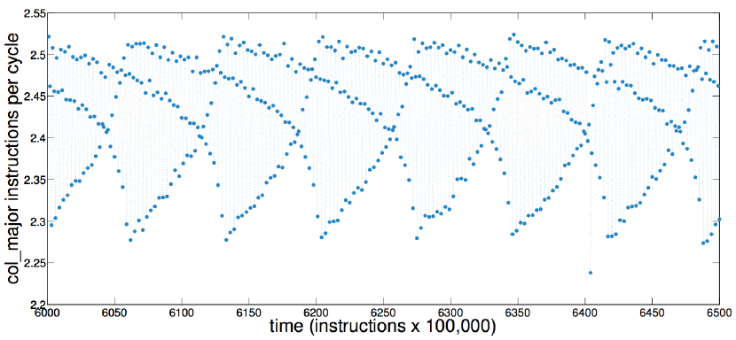
A small change in the code can cause the dynamics to bifurcate to a periodic regime. By running different programs on the same computer, then, we can produce traces that span the whole range of the complexity spectrum, from completely predictable to completely unstructured—which makes this an ideal testbed for this study222Predicting the state of a computer, of course, would amount to solving the halting problem. What we are doing here is predicting computer performance, which does not violate the Rice-Shapiro theorem Hopcroft et al. (2007)..
The time-series data sets for these experiments were collected on an Intel Core® i7-2600-based machine. We gathered performance traces during the execution of three different programs—the simple col_major loop whose performance is depicted in Figure 1 and two more-complex programs: one from the SPEC 2006CPU benchmark suite (403.gcc), and one from the LAPACK linear algebra package (dgesdd). In all of these experiments, the scalar observation was a measurement of the processor performance at time during the execution of each program. For statistical validation, we collected 15 performance traces from each of the three programs. For an in-depth description of the experimental setup used to gather these data, please see Garland and Bradley (2011, 2013); Alexander et al. (2010); Myktowicz et al. (2009); Mytkowicz (2010).
The SPEC CPU2006 benchmark suite Henning (2006) is a collection of complicated programs that are used in the computer-science community to assess and compare the performance of different computers. 403.gcc is a member of that suite. It is a compiler: a program that translates code written in a high-level language into a lower-level format that can be executed by the processor chip. Its behavior is far more complicated than that of col_major, as is clear from Figure 2.
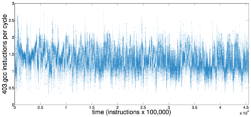
Unlike col_major, where the processor utilization is quite structured, 403.gcc’s performance appears almost random.
dgesdd is a Fortran program from the LAPACK linear algebra package Anderson et al. (1999). It calculates the singular value decomposition of a rectangular by matrix with real-valued entries. For our experiments, we chose and and generated the matrix entries randomly. The behavior of this program as it computes the singular values of this matrix is very interesting, as is clearly visible in Figure 3.
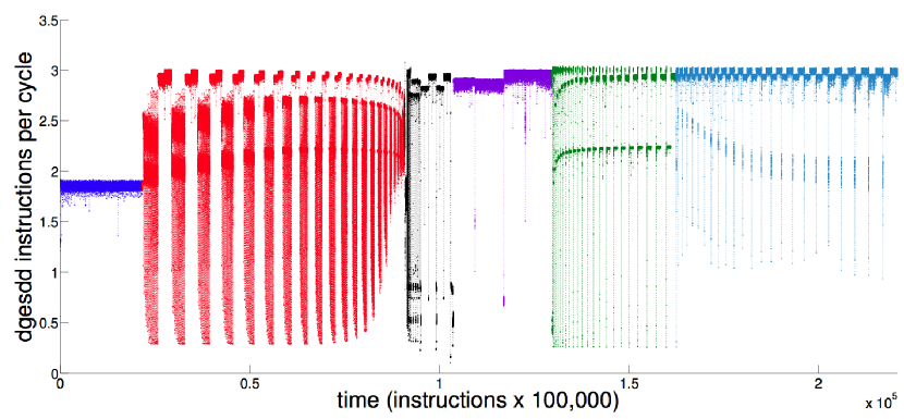
As the code moves though its different phases—diagonalizing the matrix, computing its transpose, multiplying, etc.—the processor utilization patterns change quite radically. For the first 21,000 measurements (21,000 100,000 instructions), roughly 1.8 instructions are executed per cycle, on the average, by the eight processing units on this chip. After that, the IPC moves through a number of different oscillatory regimes, which we have color-coded in the figure in order to make textual cross-references easy to track.
The wide range of behaviors in Figure 3 provides a distinct advantage, for the purposes of this paper, in that a number of different generating processes—with a wide range of complexities—are at work in different phases of a single time series. The col_major and 403.gcc traces in Figures 1 and 2 appear to be far more consistent over time—probably the result of a single generating process with consistent complexity. dgesdd, in contrast, has multiple regimes, each the result of different generating processes. To take advantage of this, we split the signal into six different segments, thereby obtaining an array of examples for the analyses in the following sections. For notational convenience, we refer to these 90 time-series data sets33315 runs, each with six regimes as dgesddi, with where corresponds to one of the six segments of the signal, ordered from left to right. These segments, which were determined visually, are shown in different colors in Figure 3. Visual decomposition is subjective, of course, particularly since the regimes exhibit some fractal structure. Thus, it may be the case that more than one generating process is at work in each of our segments. This is a factor in the discussion of Section VI.
IV Modeling
In this section, we describe the four different forecasting methods used in this study, as well as the error metric used to evaluate their predictive accuracy. These methods include:
-
•
The random-walk method, which uses the previous value in the observed signal as the forecast,
-
•
The naïve method, which uses the mean of the observed signal as the forecast,
-
•
The ARIMA (auto-regressive integrated moving average) method, a common linear forecast strategy, instatiated via the auto.arima procedure Hyndman and Khandakar (2008), and
-
•
The LMA (Lorenz method of analogues) method, which uses a near-neighbor forecast strategy on a dynamical reconstruction of the signal.
ARIMA models are based on standard linear techniques. LMA is designed to capture and exploit the deterministic structure of a signal from a nonlinear dynamical system. The naïve and random-walk methods, somewhat surprisingly, often outperform these more-sophisticated prediction strategies in the case of highly complex signals, as discussed below.
IV.1 Two Simple Prediction Strategies
A random-walk predictor simply uses the last observed measurement as the forecast: that is, the predicted value at time is calculated using the following relation:
The prediction strategy that we refer to using the term “naïve” averages the prior observations to generate the forecast:
While both of these methods are simplistic, they are not without merit. For a time series near the high end of the complexity spectrum—i.e., one that possesses very little predictive structure—these two methods can actually be the best choice. In forecasting currency exchange rates, for instance, sophisticated econometrics-based prediction models fail to consistently outperform the random-walk method Meese and Rogoff (1983); Mućk and Skrzypczyński (2012). These signals are constantly changing, noisy, and possess very little predictive structure, but their variations are not—on the average—very large, so the random-walk method’s strategy of simply guessing the last known value is not a bad choice. If a signal has a unimodal distribution with low variance, the naïve prediction strategy will perform quite well—even if the signal is highly complex—simply because the mean is a good approximation of the future behavior. Moreover, the naïve prediction strategy’s temporal average effects a low-pass filtering operation, which can mitigate the complexity in signals with very little predictive structure.
Both of these methods have significant weaknesses, however. Because they do not model the temporal patterns in the data, or even the distribution of its values, they cannot track changes in that structure. This causes them to fail in a number of important situations. Random-walk strategies are a particularly bad choice for time series that change significantly at every time step. In the worst case—a large-amplitude square wave whose period is equivalent to twice the sample time—a random-walk prediction would be exactly 180 degrees out of phase with the true continuation. The naïve method would be a better choice in this situation, since it would always split the difference. It would, however, perform poorly when a signal has a number of long-lived regimes that have significantly different means. In this situation, the inertia of the naïve method’s accumulating mean is a liability and the agility of the random-walk method is an advantage, since it can respond quickly to regime shifts.
Of course, methods that could capture and exploit the geometry of the data and/or its temporal patterns would be far more effective in the situations described in the previous paragraph. The auto.arima and LMA methods introduced in Sections IV.2 and IV.3 are designed to do exactly that. However, if a signal contains little predictive structure, forecast strategies like ARIMA and LMA have nothing to work with and thus will often be outperformed by the two simple strategies described in this section. This effect is explored further in Sections IV.4 and VI.
IV.2 A Regression-Based Prediction Strategy
A simple and yet powerful way to capture and exploit the structure of data is to fit a hyperplane to the known points and then use it to make predictions. The roots of this approach date back to the original autoregressive schema Gershenfeld and Weigend (1993), which forecasts the next time step through a weighted average of past observations:
The weighting coefficients are generally computed using either an ordinary least squares approach, or with the method of moments using the Yule-Walker equations. To account for noise in the data, one can add a so-called “moving average” term to the model; to remove nonstationarities, one can detrend the data using a differencing operation. A strategy that incorporates all three of these features is called a nonseasonal ARIMA model. If evidence of periodic structure is present in the data, a seasonal ARIMA model, which adds a sampling operation that filters out periodicities, can be a good choice.
There is a vast amount of theory and literature regarding the construction and use of models of this type; we refer the reader to Brockwell and Davis (2002) for an in-depth exploration. For the purposes of this paper, where the goal is to explore the relationship between predictability and complexity across a broad array of forecast strategies, seasonal ARIMA models are a good exemplar of the class of linear predictors. Fitting such a model to a dataset involves choosing values for the various free parameters in the autoregressive, detrending, moving average, and filtering terms. We employ the automated fitting techniques described in Hyndman and Khandakar (2008) to accomplish this, producing what we will call an “auto.arima model” in the rest of this paper. This procedure uses sophisticated methods—KPSS unit-root tests Kwiatkowski et al. (1992), a customization of the Canova-Hansen test Canova and Hansen (1995), and the Akaike information criterion Akaike (1974), conditioned on the maximum likelihood of the model fitted to the detrended data—to select good values for the free parameters of the ARIMA model.
ARIMA forecasting is a common and time-tested procedure. Its adjustments for seasonality, nonstationarity, and noise make it an appropriate choice for short-term predictions of time-series data generated by a wide range of processes. If information is being generated and/or transmitted in a nonlinear way, however, a global linear fit is inappropriate and ARIMA forecasts can be inaccurate. Another weakness of this method is prediction horizon: an ARIMA forecast is guaranteed to converge (to the mean, to a constant value, or to a linear trend) after some number of predictions, depending on model order. To sidestep this issue, we build forecasts in a stepwise fashion: i.e., fit the auto.arima model to the existing data, use that model to perform a one-step prediction, rebuild the auto.arima model using the latest observations, and iterate until the desired prediction horizon is reached. For consistency, we take the same approach with the other three models in this study as well, even though doing so amounts to artificially hobbling LMA.
IV.3 A Nonlinear Prediction Strategy
When the temporal progressions in a time series are produced by a deterministic nonlinear process, one can use a technique called delay-coordinate embedding to model the structure of the information generation and transmission occurring in the underlying process, then use that reconstruction to generate forecasts. This section discusses the theory and implementation of a prediction strategy that is based on this idea.
Delay-coordinate embedding Packard et al. (1980); Sauer et al. (1991); Takens (1981) allows one to reconstruct a dynamical system’s full state-space dynamics from a scalar time-series measurement—provided that some conditions hold regarding those data. Specifically, if the underlying dynamics and the measurement function—the mapping from the unknown state vector to the observed value —are both smooth and generic, Takens Takens (1981) formally proves that the delay-coordinate map
from a -dimensional smooth compact manifold to is a diffeomorphism on : in other words, that the reconstructed dynamics and the true (hidden) dynamics have the same topology. This is an extremely powerful result; among other things, it means that one can model the full system dynamics, up to diffeomorphism, without measuring—or even knowing—anything about the state variables.
The first step in the delay-coordinate embedding process is to estimate values for the two free parameters in the map: the delay and the dimension . We follow standard procedures for this, choosing the first minimum in the time-delayed mutual information as an estimate of Fraser and Swinney (1986) and using the false-near(est)-neighbor method of Kennel et al. (1992) to estimate . Some example plots of data from Figures 1-3, embedded following this procedure, are shown in Figure 4.
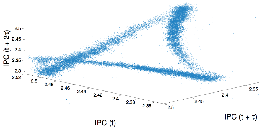
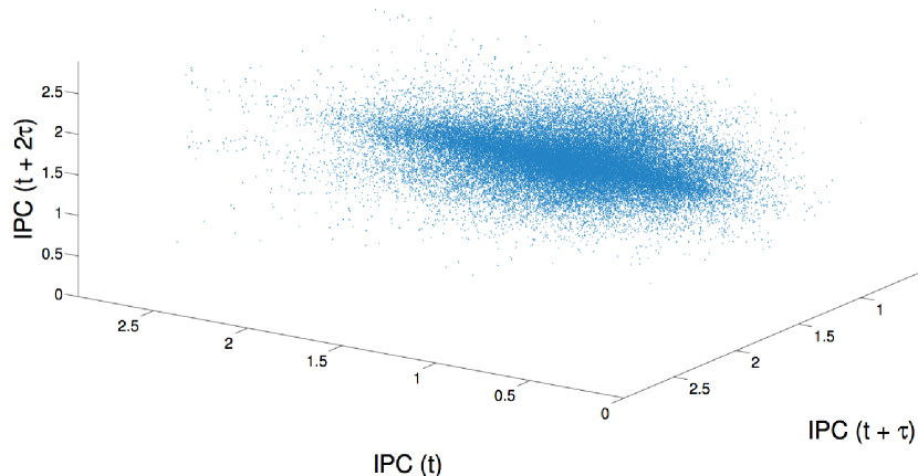
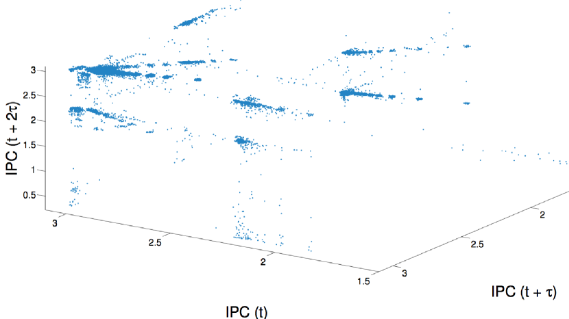
Geometric structure in these kinds of plots is an indication of structure in the information generation/transmission process that produced the time series. The dynamical systems community has developed a number of methods that leverage this structure to generate predictions (e.g., Weigend and Gershenfeld (1993); Casdagli and Eubank (1992); Smith (1992)). One of the most straightforward of these is the Lorenz method of analogues (LMA), which is essentially nearest-neighbor prediction in the embedded444Lorenz’s original formulation used the full system state space; this method was first extended to embedded dynamics by Pikovsky Pikovsky (1986), but is also related to the prediction work of Sugihara & May Sugihara and May (1990) space Lorenz (1969). Even this simple algorithm—which builds predictions by finding the nearest neighbor in the embedded space of the given point, then taking that neighbor’s path as the prediction—provides remarkably accurate forecasts when the generating process is a deterministic dynamical system.
Since LMA does not rest on an assumption of linearity (as ARIMA models do), it can handle both linear and nonlinear processes. If the underlying generating process is nondeterministic, however, it can perform poorly. Figure 4(b), for instance, appears to contain little structure, so one might not expect LMA to work well on this signal. More structure appears to be present in Figure 4(c), but this reconstruction also appears to contain some noise. The question as to how much structure is present in a reconstruction, and how much of that structure can be captured and used by LMA, is apropos of the central question treated in this paper. It may be that 403.gcc has some redundancy that LMA cannot exploit, or that the structure in dgesdd5 is effectively obfuscated, from the standpoint of the LMA method, by noise.
Without any knowledge of the generating process, answers to these questions can only be derived from the data, with all of the attendant problems (noise, sampling issues, and so on). By quantifying the balance between redundancy, predictive structure, and entropy for these real-valued time series—as shown in Section VI—we can begin to answer these questions in an effective and practical manner.
IV.4 Assessing Prediction Accuracy
To study the relationship between predictability and complexity, we use the four methods outlined above to generate predictions of all 120 traces described in Section III, then calculate the error of the predictions with respect to the true continuations. Specifically, we split each time series into two pieces: the first 90%, referred to here as the “initial training” signal and denoted , and the last 10%, known as the “test” signal . The initial training signal is used to build the model, following the procedures described in the previous section; that model is used to generate a prediction of the value of , which is then compared to the true continuation, . The model is then rebuilt using and the process repeats times, out to the end of the observed time series. This “one step prediction” process is not technically necessary in the LMA method, whose ability to generate accurate predictions is limited only by the positive Lyapunov exponents of the system. However, the performance of the other three methods used here will degrade severely if the associated models are not periodically rebuilt. In order to make the comparison fair, we used an iterative one-step prediction schema for all four methods. This has the slightly confusing effect of causing the “test” signal to be used both to assess the accuracy of each model and for periodic refitting.
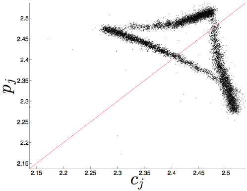
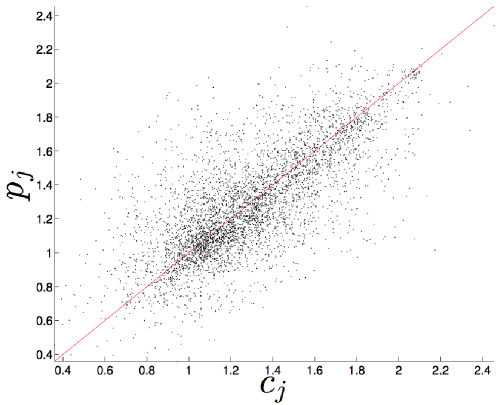
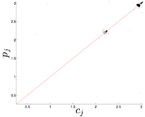
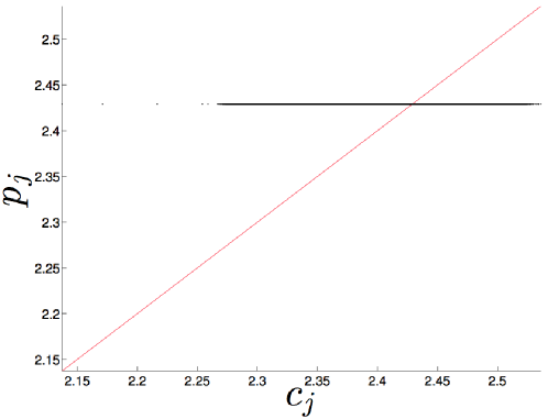
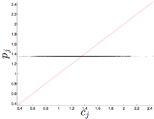
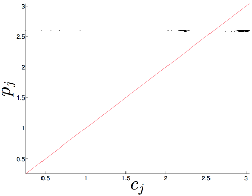
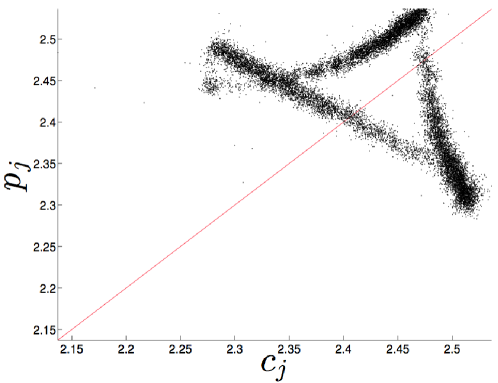
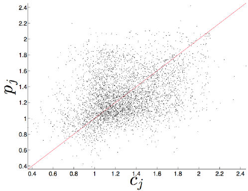
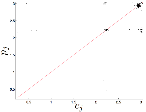
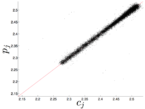
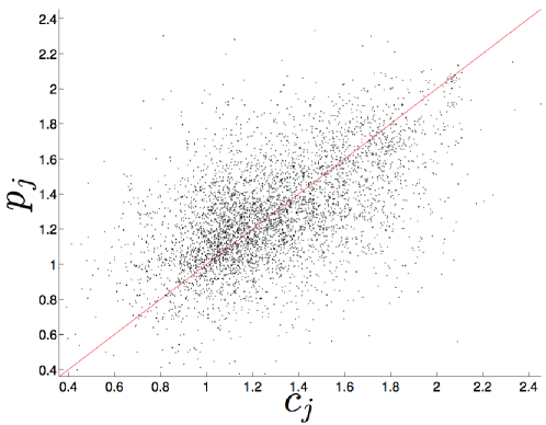
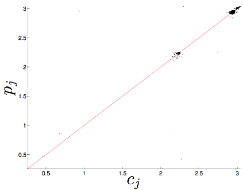
Figure 5 shows example forecasts made using all four methods for the col_major, 403.gcc, and dgesdd5 time series.
| col_major | 403.gcc | dgesdd5 | |
|---|---|---|---|
|
random walk |
|
|
|
|
naïve |
|
|
|
|
auto.arima |
|
|
|
|
LMA |
|
|
|
In these images, the vertical axis is the prediction and the horizontal axis is the true continuation . On such a plot, a perfect prediction would lie on the diagonal. LMA, for instance, generates a very accurate prediction of the col_major data, while auto.arima does not. Horizontal lines result when a constant predictor like the naïve method is used on a non-constant signal. Point clouds reflect the structure of the distribution of the errors—roughly normally distributed, for example, in the case of LMA on 403.gcc. Note that the shapes of some of the plots in Figure 5 (e.g., random walk and auto.arima on col_major) are reminiscent of the projected embedding in Figure 4(a). Indeed, for a random-walk predictor, a vs. plot is technically equivalent to a two-dimensional embedding with . For auto.arima, the correspondence is not quite as simple, since the values are linear combinations of a number of past values of the , but the effect is largely the same555The temporal ordering of the points on the auto.arima vs. plot does not match that of a projected embedding of the time series, however..
As a numerical measure of prediction accurary, we calculate the mean absolute scaled error (MASE) between the true and predicted signals:
This error metric was introduced in Hyndman and Koehler (2006) as a “generally applicable measurement of forecast accuracy without the problems seen in the other measurements.” Like many error metrics, MASE is a normalized measure: the scaling term in the denominator is the average in-sample forecast error for a random-walk prediction over the initial training signal . That is, MASE means that the prediction error in question was, on the average, smaller than the average error of a random-walk forecast on the training data. Analogously, MASE means that the corresponding prediction method did worse, on average, than the random-walk method. While its comparative nature is somewhat different than traditional metrics like normalized root mean squared error, MASE has the significant advantage of allowing one to make a fair comparison across varying methods, prediction horizons, and signal scales—attributes that are key to any broad study of predictability.
MASE scores for all 360 experiments are tabulated in the four middle columns in Table 1.
| Signal | RW MASE | naïve MASE | auto.arima MASE | LMA MASE | WPE |
|---|---|---|---|---|---|
| col_major | |||||
| 403.gcc | |||||
| dgesdd1 | |||||
| dgesdd2 | |||||
| dgesdd3 | |||||
| dgesdd4 | |||||
| dgesdd5 | |||||
| dgesdd6 |
In view of the discussion at the end of the previous paragraph, the fact that the values in the second-from-left column are not identically equal to 1.00 may be somewhat surprising. This can happen due to differences between in-sample and out-of-sample forecasting; the last 10% of dgesdd3, for instance—the out-of-sample signal—was more amenable to random-walk prediction, on the average, than the first 90%. See Section VI for a deeper discussion of this effect.
Comparing the values in Table 1 with the geometry of the plots in Figure 5, one can see some obvious correspondences. The average LMA MASE score for the col_major signals was , for instance, while auto.arima scored much worse (). That is, LMA performed roughly 20 times better on col_major signals than a random-walk predictor, while auto.arima only outperformed random walk by a factor of 1.7. This is in accordance with the visual appearance of the corresponding images in Figure 5.
In other cases, the correspondence between MASE score and the visual appearance of these kinds of plots is not so clear cut. The plots of LMA predictions of col_major and dgesdd5 both lie near the diagonal, for instance, but the corresponding MASE scores are very different: for col_major and for dgesdd5 (resp., 20 and 1.4 times better than random-walk forecasts of the same signals). This is a result of the normalization in the MASE score calculation. Recall from Section IV.1 that the random-walk method performs especially poorly on signals that oscillate rapidly. col_major fits this description, so the random-walk error on this signal—the denominator of the four MASE scores in the first row of the Table—is pathologically high, which skews those scores down. Random-walk prediction is very effective for the dgesdd5 signal, on the other hand, so the denominator is small and the MASE scores are skewed upwards.
Normalization is, as is often the case, a double-edged sword. Here, it facilitates comparisons across signals of different types and lengths, but its particular pathologies must be taken into account when analyzing the results, as discussed at more length in Section VI.
V Measuring Structural Complexity
Estimating the entropy of an arbitrary, real-valued time series is a significant challenge. Our approach to this problem, which is the topic of this section, draws upon methods and results from a variety of fields including time-series analysis, dynamical systems, and stochastic processes.
For the purposes of this paper, we view the Shannon entropy—in particular its growth rate with respect to word length (the Shannon entropy rate)—as a measure of complexity and unpredictability in a time series. Time-series consisting of i.i.d. random variables, such as white noise, have maximal entropy rates, whereas highly structured time-series, for example periodic, have very low (or zero) entropy rates. A time series with a high entropy rate is almost completely unpredictable; conversely, one with low entropy rate is often quite predictable. This can be made more rigorous: Pesin’s relation Pesin (1977) states that in chaotic dynamical systems, the Kolmogorov-Sinai (KS) entropy is equal to the sum of the positive Lyapunov exponents, . The Lyapunov exponents directly quantify the rate at which nearby states of the system diverge with time: . The faster the divergence, the larger the entropy. The KS entropy is defined as the supremum of the Shannon entropy rates of all partitions Petersen (1989). The partition that achieves this supremum is the generating partition discussed in Section II.
From a different point of view, we can consider the information (as measured by the Shannon entropy) contained in a single observable, say the present, of the system. This information can be partitioned into two components: the information shared with past observations—e.g., the mutual information between the past and present—and the information in the present that is not contained in the past (aka “the conditional entropy of the present given the past”). The first part is known as the redundancy: information in the present that is also in the past. The second part is the aforementioned Shannon entropy rate. It seems obvious that the more redundancy in a signal, the more predictable it should be. And the specific form of the redundancy should dictate whether a particular prediction method will work well or poorly on the corresponding signal. A linear method cannot capture or make use of nonlinear redundancy, for instance. This issue—which has been explored extensively using clean data and/or systems where the generating process is known, but not so much with empirical data from unknown systems—is central to the claims in this paper and the discussion in the following section.
Previous approaches to measuring temporal complexity via the Shannon entropy rate Shannon (1951); Mantegna et al. (1994) required categorical data: for some finite or countably infinite alphabet . Data taken from real-world systems are, however, effectively666Measurements from finite-precision sensors are discrete, but data from modern high-resolution sensors are, for the purposes of entropy calculations, effectively continuous. real-valued. To analyze real-valued data using a method that requires categorical values, one must discretize the data—typically by binning. Unfortunately, this is rarely a good solution, as the binning of the values introduces spurious dynamics Bollt et al. (2001). The field of symbolic dynamics offers discretization methods that do not disturb the intrinsic behavior. These methods are, however, fragile in the face of noise; worse yet, they require knowledge of the underlying system. This is inappropriate in our context, where the target of study is experimental time-series data.
Bandt and Pompe introduced the permutation entropy (PE) as a “natural complexity measure for time series” Bandt and Pompe (2002). The permutation entropy employs a method of discretizing real-valued time series that follows the intrinsic behavior of the system under examination. It has many advantages, including being robust to observational noise, and its application does not require any knowledge of the underlying mechanisms. Rather than looking at the statistics of sequences of values, as is done when computing the Shannon entropy, permutation entropy looks at the statistics of the orderings of sequences of values using ordinal analysis. Ordinal analysis of a time series is the process of mapping successive time-ordered elements of a time series to their value-ordered permutation of the same size. By way of example, if then its ordinal pattern, , is since . The ordinal pattern of the permutation is .
Definition (Permutation Entropy).
Given a time series . Define as all permutations of order . For each we determine the relative frequency of that permutation occurring in :
where quantifies the probability of an ordinal and is set cardinality. The permutation entropy of order is defined as
Notice that Bandt and Pompe (2002). With this in mind, it is common in the literature to normalize permutation entropy as follows: . With this convention, “low” PE is close to 0 and “high” PE is close to 1. Finally, it should be noted that the permutation entropy has been shown to be identical to the Kolmolgorov-Sinai entropy for many large classes of systems Amigó (2012), as long as observational noise is sufficiently small. As mentioned before, this is equal to the Shannon entropy rate of a generating partition of the system. This transitive chain of equalities, from permutation entropy to Shannon entropy rate via the KS entropy, allows us to approximate the redundancy—being the dual of the Shannon entropy rate—of a signal by .
Here we will be utilizing a variation of the basic permutation entropy technique, the weighted permutation entropy (WPE), which was introduced in Fadlallah et al. (2013). The intent behind the weighting is to correct for observational noise that is larger than the trends in the data, but smaller than the larger-scale features. Consider, for example, a signal that switches between two fixed points and contains some additive noise. The PE of such a signal will be dominated by the noise about the fixed points, driving it to —which in some sense hides the fact that the signal is actually quite structured. In this situation, the terms of the weighted permutation entropy are dominated by the switching rather than the stochastic fluctuations. The amplitude of the switches plays a key role in predictability, so weighting the scale of ordinal changes is important for quantifying predictive structure accurately. To accomplish this, WPE takes into account the weight of a permutation:
where is a sequence of values , and is the arithmetic mean of those values.
The weighted probability of a permutation is defined as:
where is 1 if and 0 otherwise. Effectively, this weighted probability enhances permutations that are involved in “large” features and de-emphasizes permutations that are small in amplitude relative to the features of the time series. Using the standard form of an entropy, the weighted permutation entropy is:
which can also be normalized by dividing by , making . This normalization is used in all the results that follow.
In practice, calculating permutation entropy and weighted permutation entropy involves choosing a good value for the word length . The primary consideration in that choice is that the value be large enough that forbidden ordinals are discovered, yet small enough that reasonable statistics over the ordinals are gathered. If an average of 100 counts per ordinal is considered to be sufficient, for instance, then . In the literature, is a standard choice—generally without any formal justification. In theory, the permutation entropy should reach an asymptote with increasing , but that can require an arbitrarily long time series. In practice, what one should do is calculate the persistent permutation entropy by increasing until the result converges, but data length issues can intrude before that convergence is reached. We used this approach, which we believe strikes a good balance between accurate ordinal statistics and finite-data effects, to choose values for the experiments in the following section.
VI Predictability, Complexity, and Permutation Entropy
In this section, we offer an empirical validation of the two findings introduced in Section I, namely:
-
1.
The weighted permutation entropy (WPE) of a noisy real-valued time series from an unknown system is correlated with prediction accuracy—i.e., the predictable structure in an empirical time-series data set can be quantified by its WPE.
-
2.
The relationship between WPE and mean absolute scaled error (MASE) is a useful empirical heuristic for identifying mismatches between prediction models and time-series data—i.e., when there is structure in the data that the model is unable to exploit.
The experiments below involve four different prediction methods applied to time-series data from eight different systems: col_major, 403.gcc, and the six different segments of the dgesdd signal in Figure 3. The objective of these experiments was to explore how prediction accuracy is related to WPE. Working from the first 90% of each signal, we generated a prediction of the last 10% using the random-walk, naïve, auto.arima, and LMA prediction methods, as described in Section IV.4, then calculated the MASE value of those predictions. We also calculated the WPE of each time series using a wordlength chosen via the procedure described at the end of Section V. In order to assess the run-to-run variability of these results, we repeated all of these calculations on 15 separate trials: i.e., 15 different runs of each program.
Figure 6 plots the WPE values versus the corresponding MASE values of the best prediction for each of the 120 time series in this study.
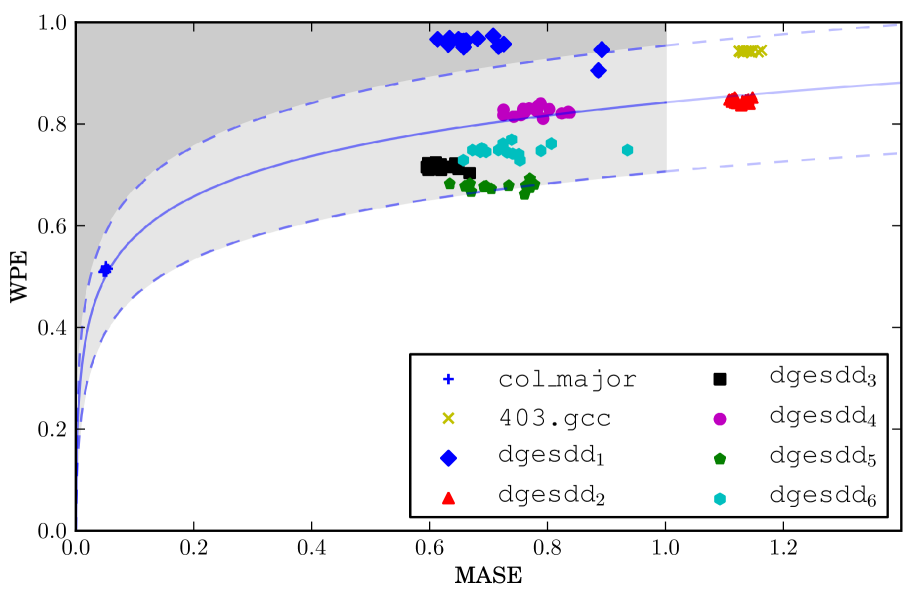
There is an obvious upward trend, which is consistent with the notion that there is a pattern in the WPE-MASE relationship. However, a simple linear fit is a bad idea here. First, any signal with zero entropy should be perfectly predictable (i.e., MASE ), so any curve fitted to these data should pass through the origin. Moreover, WPE does not grow without bound, so one would expect the patterns in the WPE-MASE pairs to reach some sort of asymptote. For these reasons, we chose to fit a function of the form to these points777The specific values of the coefficients are and ., with WPE and MASE. The solid curve in the figure shows this fit; the dashed curves show the standard deviation of this model in its parameter space: i.e., with one standard deviation on each of the two parameters. Points that fall within this deviation volume (light grey) correspond to predictions that are comparable to the best ones found in this study; points that fall above that volume (dark grey) are better still. We chose to truncate the shaded region because of a subtle point regarding the MASE of an ideal predictor, which should not be larger than 1 unless the training and test signals are different. This is discussed at more length below.
The curves and regions in Figure 6 are a graphical representation of the first finding. This representation is, we believe, a useful heuristic for determining whether a given prediction method is well matched to a particular time series. It is not, of course, a formal result. The forecast methods and data sets used here were chosen to span the space of standard prediction strategies and the range of dynamical behaviors, but they do not cover those spaces exhaustively. Our goal here is an empirical assessment of the relationship between predictability and complexity, not formal results about a “best” predictor for a given time series. There may be other methods that produce lower MASE values than those in Figure 6, but the sparseness of the points above and below the one- region about the dashed curve in this plot strongly suggests a pattern of correlation between the underlying predictability of a time series and its WPE. The rest of this section describes these results and claims in more detail—including the measures taken to assure meaningful comparisons across methods, trials, and programs—and elaborates on the meaning of the different curves and limits in the figure.
Figure 7 shows WPE vs. MASE plots for the full set of experiments.
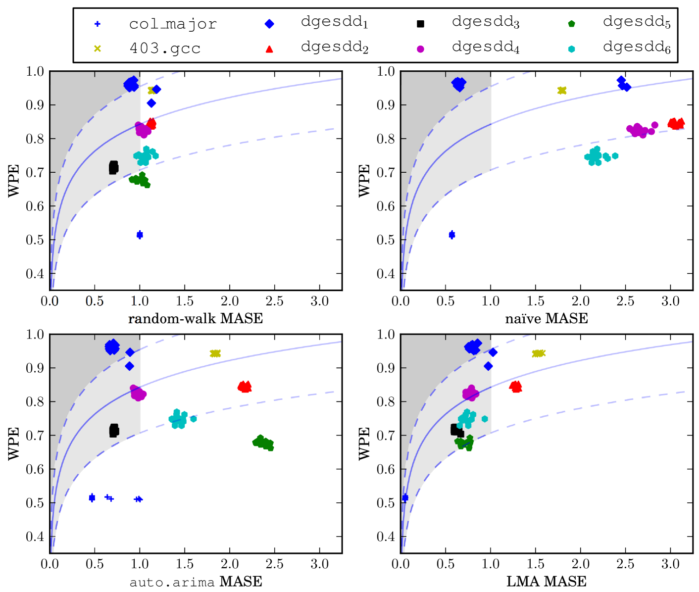
There are 15 points in each cluster, one for each trial. (The points in Figure 6 are the leftmost of the points for the corresponding trace in any of the four plots in Figure 7.) The WPE values do not vary very much across trials. For most traces, the variance in MASE scores is low as well, resulting in small, tight clusters. In some cases—auto.arima predictions of col_major, for instance—the MASE variance is larger, which spreads out the clusters horizontally. The mean MASE scores of predictions generated with the nonlinear LMA method are generally closer to the dashed curve; the auto.arima method clusters are more widely spread, the naïve clusters even more so. A few of the clusters have very high variance; these are discussed later in this section.
The main thing to note here, however, is not the details of the shapes of the clusters, but rather their positions in the four plots: specifically, the fact that many of them are to the right of and/or below the dashed curve that identifies the boundary of the shaded region. These predictions are not as good as our heuristic suggests they could be. Focusing in on any single signal makes this clear: LMA works best for dgesdd6, for instance, followed by the random-walk prediction method, then auto.arima and naïve. This provides some practical leverage: if one calculates an WPE vs. MASE value that is outside the shaded region, that should suggest that the prediction method is not well matched to the task at hand: that is, the time series has more predictive structure than the method is able to use. In the case of auto.arima on dgesdd6, for instance, one should try a different method. The position of the LMA cluster for dgesdd6, on the other hand, reflects this method’s ability to capture and exploit the structure that is present in this signal. WPE vs. MASE values like this, which fall in the shaded region, should suggest to the practitioner that the prediction method is well-suited to the task. The following discussion lays out the details that underlie these claims.
Though col_major is a very simple program, its dynamics are actually quite complicated, as discussed in Section I. Recall from Figure 5 and Table 1 that the naïve, auto.arima, and (especially) random-walk prediction methods do not perform very well on this signal. The MASE scores of these predictions are , , and , respectively, across all 15 trials. That is, naïve and auto.arima perform only times better than the random-walk method, a primitive strategy that simply uses the current value as the prediction. However, the WPE value for the col_major trials is , a signal that is in the center of the complexity spectrum described in Section I.
This disparity—WPE values that suggest a high rate of forward information transfer in the signal, but predictions with comparatively poor MASE scores—is obvious in the geometry of three of the four images in Figure 7, where the col_major clusters are far to the right of and/or below the dashed curve. Again, this indicates that these methods are not leveraging the available information in the signal. The dynamics of col_major may be complicated, but they are not unstructured. This signal is nonlinear and deterministic Myktowicz et al. (2009), and if one uses a prediction technique that is based a nonlinear model (LMA)—rather than a method that simply predicts the running mean (naïve) or the previous value (random walk), or one that uses a linear model (auto.arima)—the MASE score is much improved: . This prediction is 20 times more accurate than a random-walk forecast, which is more in line with the level of predictive structure that the low WPE value suggests is present in the col_major signal. The MASE scores of random-walk predictions of this signal are all —as one would expect—pushing those points well below the shaded region. Clearly the stationarity assumption on which this method is based does not hold for this signal.
The col_major example brings out some of the shortcomings of automated model-building processes. Note that the points are clustered very tightly in the lower left quadrant of the naïve, random-walk, and LMA plots in Figure 7, but spread out horizontally in the auto.arima plot. This is because of the way the auto.arima process builds ARIMA models Hyndman and Khandakar (2008). If a KPSS test of the time series in question indicates that it is nonstationary, the auto.arima recipe adds an integration term to the model. This test gives mixed results in the case of the col_major process, flagging five of the 15 trials as stationary and ten as nonstationary. We conjectured that ARIMA models without an integration term perform more poorly on these five signals, which increases the error and thereby spreads out the points. We tested this hypothesis by forcing the inclusion of an integration term in the five cases where a KPSS test indicated that such a term was not needed. This action removed the spread, pushing all 15 of the col_major auto.arima points in Figure 7 into a tight cluster.
The discussion in the previous paragraph highlights the second finding of this paper: the ability of our proposed heuristic to flag inappropriate models. auto.arima is an automated, mechanical procedure for choosing parameters for an ARIMA model of a given data set. While the tests and criteria employed by this algorithm (Section IV.2) are sophisticated, the results can still be sub-optimal—if the initial space of models being searched is not broad enough, for instance, or if one of the preliminary tests gives an erroneous result. auto.arima always returns a model, and it can be very hard to detect when that model is bad. Our results suggest a way to do so: if the MASE score of an auto-fitted model like auto.arima is out of line with the WPE value of the data, that can be an indication of inappropriateness in the order selection and parameter estimation procedure.
The WPE of dgesdd5 () is higher than that of col_major. This indicates that the rate of forward information transfer of the underlying process is lower, but that time-series data observed from this system still contain a significant amount of structure that can, in theory, be used to predict the future course of the time series. The MASE scores of the naïve and auto.arima predictions for this system are and , respectively: that is, 20.87 and 2.37 times worse than a simple random-walk forecast of the training set portions of the same signals888The naïve MASE score is large because of the bimodal nature of the distribution of the values of the signal, which makes guessing the mean a particularly bad strategy. The same thing is true of the dgesdd3 signal.. As before, the positions of these points on a WPE vs. MASE plot—significantly below and to the right of the shaded region—should suggest to a practitioner that a different method might do better. Indeed, for dgesdd5, the LMA method produces a MASE score of and a cluster of results that largely within the shaded region on the WPE-MASE plot. This is consistent with our second finding: the LMA method can capture and reproduce the way in which the dgesdd5 system processes information, but the naïve and auto.arima prediction methods cannot.
The WPE of 403.gcc is higher still: . This system transmits very little information forward in time and provides almost no structure for prediction methods to work with. Here, the random-walk predictor is the best of the methods used here. This makes sense; in a fully complex signal, where there is no predictive structure to utilize, methods that depend on exploiting that structure—like ARIMA and LMA—cannot get any traction on those signals. Since fitting a hyperplane using least squares should filter out some of the noise in the signal, the fact that LMA outperforms auto.arima ( vs. ) may be somewhat counterintuitive. However, the small amount of predictive structure that is present in this signal is nonlinear (cf., Myktowicz et al. (2009)), and LMA is designed to capture and exploit that kind of structure. Note that all four 403.gcc clusters in Figure 7 are outside the shaded region; in the case of the random-walk prediction, for instance, the MASE value is . This is due to nonstationarity in the signal: in particular, differences between the training and test signals. The same effect is at work in the dgesdd2 results, for the same reasons—and visibly so, in the red segment of Figure 3, where the period and amplitude of the oscillations are decreasing.
dgesdd1—the dark blue segment of Figure 3—behaves very differently than the other seven systems in this study. Though its weighted permutation entropy is very high (), three of the four prediction methods do quite well on this signal, yielding mean MASE scores of 0.714 (auto.arima), 0.827 (LMA), and 0.933 (random walk). This pushes the corresponding clusters of points in Figure 7 well above the trend followed by the other seven signals. The reasons for this are discussed in the following paragraph. The MASE scores of the predictions that were produced by the naïve method for this system, however, are highly inconsistent. The majority of the blue diamond-shaped points on the top-right plot in Figure 7 are clustered near a MASE score of 0.6, which is better than the other three methods. In five of the 15 dgesdd1 trials, however, there were step changes in the signal. This is a different nonstationarity than in the case of col_major—large jump discontinuities rather than small shifts in the baseline—and not one that we were able to handle by simply forcing the ARIMA model to include a particular term. The naïve method has a very difficult time with signals like this, particularly if there are multiple step changes. This raised the MASE scores of these trials, pushing the corresponding points to the right999This includes the cluster of three points near MASE , as well as two points that are beyond the domain of the graph, at MASE ., and in turn raising both the mean and variance of this set of trials.
The effects described in the previous paragraph are also exacerbated by the way MASE is calculated. Recall that MASE scores are scaled relative to a random-walk forecast. There are two issues here. First, random-walk prediction works very badly on signals with frequent, large, rapid transitions. Consider a signal that oscillates from one end of its range to the other at every step. A signal like this will have a low WPE, much like col_major. However, a random-walk forecast of this signal will be 180 degrees out of phase with the true continuation. Since random-walk error appears in the denominator of the MASE score, this effect can shift points leftwards on a WPE vs. MASE plot, and that is exactly why the dgesdd1 clusters in Figure 7 are above the dashed curve. This time series, part of which is shown in closeup in Figure 8,
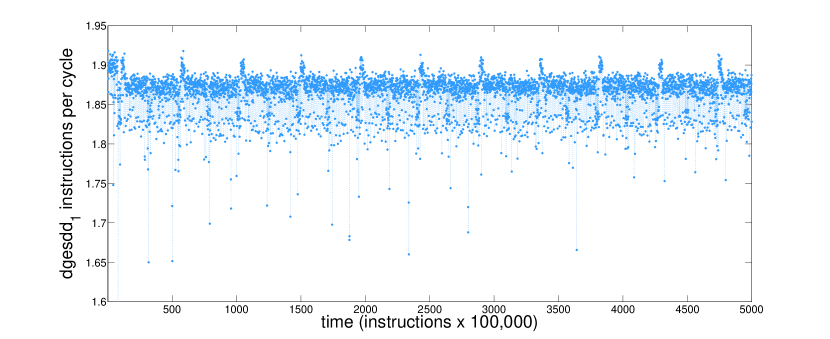
is not quite to the level of the worst-case signal described above, but it still poses a serious challenge to random-walk prediction. It is dominated by a noisy regime (between 1.86 and 1.88 on the vertical scale in Figure 8), punctuated by short excursions above 1.9. In the former regime, which makes up more than 80% of the signal, there are frequent dips to 1.82 and occasional larger dips below 1.8. These single-point dips are the bane of random-walk forecasting. In this particular case, roughly 40% of the forecasted points are off by the width of the associated dip, which skews the associated MASE scores. Signals like this are also problematic for the naïve prediction strategy, since the outliers have significant influence on the mean. This compounds the effect of the skew in the scaling factor and exacerbates the spread in the dgesdd1 MASE values.
The second effect that can skew MASE scores is nonstationarity. Since this metric is normalized by the error of a random-walk forecast on the training signal, differences between the test signal and training signal can create issues. This is why the MASE values in Table 1 are not identically one for every random-walk forecast of every time series: the last 10% of these signals is significantly different from the first 90%. The deviation from 1.00 will depend on the process—whether it has multiple regimes, what those regimes look like, and how it switches between them—as well as the experimental setup (e.g., sensor precision and data length). For the processes studied here, these effects do not cause the MASE values to exceed 1.15, but pathological situations (e.g., a huge switch in scale right at the training/test signal boundary, or a signal that simply grows exponentially) could produce higher values. This suggests another potentially useful heuristic: if the MASE of a random-walk prediction of a time series is significantly different from 1, this could be an indication that the signal is nonstationary. We are in the process of exploring this idea and its relationship to the DVS graphs mentioned in the fourth paragraph of Section II.
The curves in Figures 6 and 7 were determined from finite sets of methods and data. We put a lot of thought and effort into making these sets representative and comprehensive. The forecast methods involved range from the simple to the sophisticated; the time-series data analyzed in this section was sampled from a system whose behavior spans the dynamical behavior space. While we are cautiously optimistic about the generality of our conclusions, more exploration will be required before we can make any such claim. Our preliminary work along those lines shows that data from the Hénon map Hénon (1976), the Lorenz system Lorenz (1963), the SFI A data set101010This dataset can be retrieved from http://www-psych.stanford.edu/~andreas/Time-Series/SantaFe.html. Weigend and Gershenfeld (1993), and a random-walk process all fall within the one- volume of the fit in Figures 6 and 7 region, as do various nonlinear transformations of dgesdd2, dgesdd5 and dgesdd6.
Of course, the geometry of the curves and bounds in these figures do not necessarily extend to other error metrics. The positions of the WPE vs. error points—and the reasons to choose a particular function to fit to them or impute theoretical bounds on the meaning of the results—may change if one calculates error using a procedure other than the one described in Section IV.4. The MASE error metric, as discussed above, has its weaknesses. Even so, we concur with Hyndman and Koehler (2006) that it is an effective way to compare prediction error across time-series data of different lengths and different scales, and we are convinced by the extensive evaluations that are offered in that paper, as well as the comparisons of MASE to other metrics, that its strengths far outweigh its weaknesses.
VII Conclusions & Future Work
Forecast strategies that are designed to capture predictive structure are ineffective when signal complexity outweighs information redundancy. This poses a number of serious challenges in practice. Without knowing anything about the generating process, it is difficult to determine how much predictive structure is present in a noisy, real-world time series. And even if predictive structure exists, a given forecast method may not work, simply because it cannot exploit the structure that is present (e.g., a linear model of a nonlinear process). If a forecast model is not producing good results, a practitioner needs to know why: is the reason that the data contain no predictive structure—i.e., that no model will work—or is the model that s/he is using simply not good enough?
In this paper, we have argued that redundancy is a useful proxy for the inherent predictability of an empirical time series. To operationalize that relationship, we use an approximation of the Kolmogorov-Sinai entropy, estimated using a weighted version of the permutation entropy of Bandt and Pompe (2002). This WPE technique—an ordinal calculation of forward information transfer in a time series—is ideal for our purposes because it works with real-valued data and is known to converge to the true entropy value. Using a variety of forecast models and more than 150 time-series data sets from experiments and simulations, we have shown that prediction accuracy is indeed correlated with weighted permutation entropy: the higher the WPE, in general, the higher the prediction error. The relationship is roughly logarithmic, which makes theoretical sense, given the nature of WPE, predictability, and MASE.
An important practical corollary to this empirical correlation of predictability and WPE is a practical strategy for assessing appropriateness of forecast methods. If the forecast produced by a particular method is poor but the time series contains a significant amount of predictive structure, one can reasonably conclude that that method is inadequate to the task and that one should seek another method. The nonlinear LMA method, for instance, performs better in most cases because it is more general. (This is particularly apparent in the col_major and dgesdd5 examples.) The naïve method, which simply predicts the mean, can work very well on noisy signals because it effects a filtering operation. The simple random-walk strategy outperforms LMA, auto.arima, and the naïve method on the 403.gcc signal, which is extremely complex—i.e., extremely low redundancy.
The curves and shaded regions in Figures 6 and 7 generalize and operationalize the discussion in the previous paragraph. These geometric features are a preliminary, but potentially useful, heuristic for knowing when a model is not well-matched to the task at hand: a point that is below and/or to the right of the shaded regions on a plot like Figure 7 indicates that the time series has more predictive structure than the forecast model can capture and exploit—and that one would be well advised to try another method.
These curves were determined empirically using a specific error metric and a finite set of forecast methods and time-series traces. If one uses a different error metric, the geometry of the heuristic will be different—and may not even make sense, if one uses a metric that does not support comparison across different time series. And while the methods and traces used in this study were chosen to be representative of the practice, they are of course not completely comprehensive. It is certainly possible, for instance, that the nonlinear dynamics of computer performance is subtly different from the nonlinear dynamics of other systems. Our preliminary results on other systems (Hénon, Lorenz, a random-walk process, SFI “A”, nonlinear transformations of the computer performance data) lead us to believe that our results will generalize beyond the examples described in this paper. We are in the process of following up on that exploration with a broader study of data, forecast methods, and error metrics.
Nonstationarity is a serious challenge in any time-series modeling problem. Any regime shift that causes a change in the predictive structure between the training signal and the test signal, for instance, may skew the MASE score and thereby affecting the utility of our heuristic. Conversely, though, a MASE score of a random-walk prediction that is significantly different from 1.0—as mentioned at end of the previous section—could potentially be a good indicator of nonstationarity.
Detecting regime shifts—and adapting prediction models accordingly—is an important area of future work. Indeed, one of the first applications of permutation entropy was to recognize the regime shift in brainwave data that occurs when someone has a seizure Cao et al. (2004). Recall that the signal in Figure 3 was especially useful for the study in this paper because it contained a number of different regimes. We segmented this signal visually, but one could imagine using some combination of WPE and MASE to do so instead (e.g., in a sliding window across the time series). Automating regime-shift detection would be an important step towards a fully adaptive modeling strategy, where old models are discarded and new ones are rebuilt whenever the time series enters a new regime. Our WPE vs. MASE results could be particularly powerful in this scenario, as their values could not only help with regime-shift detection, but also suggest what kind of model might work well in each new regime. Of particular interest would be the class of so-called hybrid systems Goebel et al. (2009), which exhibit discrete transitions between different continuous regimes—e.g., a lathe that has an intermittent instability or traffic at an internet router, whose characteristic normal traffic patterns shift radically during an attack. Effective modeling and prediction of these kinds of systems is quite difficult; doing so adaptively and automatically—in the manner that is alluded to at the end of the previous paragraph—would be an interesting challenge.
Acknowledgment
This work was partially supported by NSF grant #CMMI-1245947 and ARO grant #W911NF-12-1-0288. We would also like to acknowledge the Santa Fe Institute whose interdisciplinary halls created a place for this work to be born, and the anonymous reviewers whose comments strengthened the presentation.
References
- Crutchfield and Feldman (2003) J. P. Crutchfield and D. P. Feldman, Chaos 13, 25 (2003).
- Lind and Marcus (1995) D. Lind and B. Marcus, An Introduction to Symbolic Dynamics and Coding (Cambridge University Press, 1995).
- Shalizi and Crutchfield (2001) C. R. Shalizi and J. P. Crutchfield, J. Stat. Phys. 104, 817 (2001).
- Bandt and Pompe (2002) C. Bandt and B. Pompe, Phys. Rev. Lett. 88, 174102 (2002).
- Bollt et al. (2001) E. M. Bollt, T. Stanford, Y.-C. Lai, and K. Życzkowski, Phys. D 154, 259 (2001).
- Yule (1927) U. G. Yule, Phil. Trans. R. Soc. London A 226, 267 (1927).
- Smith (1992) L. A. Smith, Phys. D 58, 50 (1992).
- Gershenfeld and Weigend (1993) N. Gershenfeld and A. Weigend, in Time Series Prediction: Forecasting the Future and Understanding the Past, edited by A. Weigend and N. Gershenfeld (Addison-Wesley, 1993).
- Casdagli (1992) M. Casdagli, J. R. Stat. Soc. B 54, 303 (1992).
- Shannon (1951) C. E. Shannon, Bell Syst. Tech. J. 30, 50 (1951).
- Mantegna et al. (1994) R. N. Mantegna, S. V. Buldyrev, A. L. Goldberger, S. Havlin, C. K. Peng, M. Simons, and H. E. Stanley, Phys. Rev. Lett. 73, 3169 (1994).
- Eisele (1999) M. Eisele, J. Phys. A 32, 1533 (1999).
- Haven et al. (2005) K. Haven, A. Majda, and R. Abramov, J. Comput. Phys. 206, 334 (2005).
- Boffetta et al. (2002) G. Boffetta, M. Cencini, M. Falcioni, and A. Vulpiani, Phys. Rep. 356, 367 (2002).
- Myktowicz et al. (2009) T. Myktowicz, A. Diwan, and E. Bradley, Chaos 19, 033124 (2009).
- Hopcroft et al. (2007) J. Hopcroft, R. Motwani, and J. Ullman, Introduction to automata theory, languages, and computation (Pearson/Addison Wesley, 2007).
- Garland and Bradley (2011) J. Garland and E. Bradley, in Advances in Intelligent Data Analysis X, Lecture Notes in Computer Science, Vol. 7014, edited by J. Gama, E. Bradley, and J. Hollmén (Springer Berlin/Heidelberg, 2011) pp. 173–184.
- Garland and Bradley (2013) J. Garland and E. Bradley, in Advances in Intelligent Data Analysis XII, Lecture Notes in Computer Science, Vol. 8207, edited by A. Tucker, F. Höppner, A. Siebes, and S. Swift (Springer Berlin/Heidelberg, 2013) pp. 210–222.
- Alexander et al. (2010) Z. Alexander, T. Mytkowicz, A. Diwan, and E. Bradley, in Advances in Intelligent Data Analysis IX, Lecture Notes in Computer Science, Vol. 6065, edited by N. Adams, M. Berthold, and P. Cohen (Springer Berlin/Heidelberg, 2010).
- Mytkowicz (2010) T. Mytkowicz, Ph.D. thesis, University of Colorado (2010).
- Henning (2006) J. L. Henning, SIGARCH Comput. Archit. News 34, 1 (2006).
- Anderson et al. (1999) E. Anderson, Z. Bai, C. Bischof, S. Blackford, J. Demmel, J. Dongarra, J. Du Croz, A. Greenbaum, S. Hammarling, A. McKenney, and D. Sorensen, LAPACK Users’ Guide, 3rd ed. (Society for Industrial and Applied Mathematics, Philadelphia, PA, 1999).
- Hyndman and Khandakar (2008) R. J. Hyndman and Y. Khandakar, J. Stat. Softw. 27, 1 (2008).
- Meese and Rogoff (1983) R. Meese and K. Rogoff, J. Int. Econ. 14, 3 (1983).
- Mućk and Skrzypczyński (2012) J. Mućk and P. Skrzypczyński, National Bank of Poland Working Papers 127 (2012) (unpublished).
- Brockwell and Davis (2002) P. J. Brockwell and R. A. Davis, Introduction to Time Series and Forecasting (Springer-Verlag, 2002).
- Kwiatkowski et al. (1992) D. Kwiatkowski, P. C. B. Phillips, P. Schmidt, and Y. Shin, J. Econometrics 54, 159 (1992).
- Canova and Hansen (1995) F. Canova and B. E. Hansen, J. Bus. Econ. Stat. 13, 237 (1995).
- Akaike (1974) H. Akaike, IEEE Trans. Automat. Contr. 19, 716 (1974).
- Packard et al. (1980) N. H. Packard, J. P. Crutchfield, J. D. Farmer, and R. S. Shaw, Phys. Rev. Lett. 45, 712 (1980).
- Sauer et al. (1991) T. Sauer, J. Yorke, and M. Casdagli, J. Stat. Phys. 65, 579 (1991).
- Takens (1981) F. Takens, in Dynamical Systems and Turbulence, Warwick 1980, Vol. 898, edited by D. Rand and L.-S. Young (Springer Berlin/Heidelberg, 1981) pp. 366–381.
- Fraser and Swinney (1986) A. M. Fraser and H. L. Swinney, Phys. Rev. A 33, 1134 (1986).
- Kennel et al. (1992) M. B. Kennel, R. Brown, and H. D. I. Abarbanel, Phys. Rev. A 45, 3403 (1992).
- Weigend and Gershenfeld (1993) A. Weigend and N. Gershenfeld, eds., Time Series Prediction: Forecasting the Future and Understanding the Past (Santa Fe Institute, 1993).
- Casdagli and Eubank (1992) M. Casdagli and S. Eubank, eds., Nonlinear Modeling and Forecasting (Addison Wesley, 1992).
- Pikovsky (1986) A. Pikovsky, Sov. J. Commun. Technol. Electron. 31, 911 (1986).
- Sugihara and May (1990) G. Sugihara and R. M. May, Nature 344, 734 (1990).
- Lorenz (1969) E. N. Lorenz, J. Atmos. Sci. 26, 636 (1969).
- Hyndman and Koehler (2006) R. J. Hyndman and A. B. Koehler, Int. J. Forecasting 22, 679 (2006).
- Pesin (1977) Y. B. Pesin, Russ. Math. Surv. 32, 55 (1977).
- Petersen (1989) K. Petersen, Ergodic Theory (Cambridge University Press, 1989).
- Amigó (2012) J. Amigó, Permutation Complexity in Dynamical Systems: Ordinal Patterns, Permutation Entropy and All That (Springer, 2012).
- Fadlallah et al. (2013) B. Fadlallah, B. Chen, A. Keil, and J. Príncipe, Phys. Rev. E 87, 022911 (2013).
- Hénon (1976) M. Hénon, Communications in Mathematical Physics 50, 69 (1976).
- Lorenz (1963) E. Lorenz, Journal of the Atmospheric Sciences 20, 130 (1963).
- Cao et al. (2004) Y. Cao, W. W. Tung, J. B. Gao, V. A. Protopopescu, and L. M. Hively, Phys. Rev. E 70, 046217 (2004).
- Goebel et al. (2009) R. Goebel, R. Sanfelice, and A. Teel, IEEE Control Syst. Mag. 29, 28 (2009).