Diffusion LMS over Multitask Networks

Jie Chen, , Cédric Richard,
Ali H. Sayed,
Université de Nice Sophia-Antipolis, UMR CNRS 7293, Observatoire de la Côte d’Azur
Laboratoire Lagrange, Parc Valrose, 06102 Nice - France
phone: (33) 492 076 394             fax: (33) 492 076 321
dr.jie.chen@ieee.org       cedric.richard@unice.fr
Electrical Engineering Department
University of California, Los Angeles, USA
phone: (310) 267 2142             fax: (310) 206 8495
sayed@ee.ucla.edu
The work of C. Richard was partly supported by the Agence Nationale pour la Recherche, France, (ODISSEE project, ANR-13-ASTR-0030). The work of A. H. Sayed was supported in part by NSF grants CCF-1011918 and ECCS-1407712. A short and preliminary version of this work appears in the conference publication [1].
Abstract

The diffusion LMS algorithm has been extensively studied in recent years. This efficient strategy allows to address distributed optimization problems over networks in the case where nodes have to collaboratively estimate a single parameter vector. Nevertheless, there are several problems in practice that are multitask-oriented in the sense that the optimum parameter vector may not be the same for every node. This brings up the issue of studying the performance of the diffusion LMS algorithm when it is run, either intentionally or unintentionally, in a multitask environment. In this paper, we conduct a theoretical analysis on the stochastic behavior of diffusion LMS in the case where the single-task hypothesis is violated. We analyze the competing factors that influence the performance of diffusion LMS in the multitask environment, and which allow the algorithm to continue to deliver performance superior to non-cooperative strategies in some useful circumstances. We also propose an unsupervised clustering strategy that allows each node to select, via adaptive adjustments of combination weights, the neighboring nodes with which it can collaborate to estimate a common parameter vector. Simulations are presented to illustrate the theoretical results, and to demonstrate the efficiency of the proposed clustering strategy.

Index Terms:
Multitask learning, distributed optimization, diffusion strategy, collaborative processing, stochastic performance, adaptive clustering.

I Introduction

Distributed adaptive estimation is an attractive and challenging problem that allows a collection of interconnected nodes to perform preassigned tasks from streaming measurements, such as parameter estimation. Although centralized strategies may benefit from information collected throughout a network, in most cases, distributed strategies are more robust to solve inference problems in a collaborative and autonomous manner [2].

Most recent efforts in the study of distributed estimation problems have focused on scenarios where the network is employed to collectively estimate a single parameter vector. Several strategies have been proposed for this purpose for sequential data processing over networks, including consensus strategies [3, 4, 5, 6, 7, 8, 9, 10], incremental strategies [11, 12, 13, 14, 15], and diffusion strategies [16, 17]. Diffusion strategies are particularly attractive due to their enhanced adaptation performance and wider stability ranges when constant step-sizes are used to enable continuous learning [18]. For this reason, we focus on this class of strategies in the remainder of the article. These strategies estimate a common parameter vector by minimizing, in a distributed manner, a global criterion that aggregates neighborhood cost functions. Nodes exchange information locally and cooperate only with their neighbors, without the need for sharing and requiring any global information. The resulting networks benefit from the temporal and spatial diversity of the data and end up being endowed with powerful learning and tracking abilities [18, 19]. The performance of the corresponding adaptive networks have been extensively studied in the literature, under favorable and unfavorable conditions such as model non-stationarities and imperfect communication [20, 21]. This framework has also been extended by considering more general cost functions and data models [19, 22, 23, 24, 25], by incorporating additional regularizers [26, 27, 28], or by expanding its use to other scenarios [29, 30, 31, 32].

The working hypothesis for these earlier studies on diffusion LMS strategies is that the nodes cooperate with each other to estimate a single parameter vector. We shall refer to problems of this type as single-task problems. However, many problems of interest happen to be multitask-oriented in the sense that there are multiple optimum parameter vectors to be inferred simultaneously and in a collaborative manner. The multitask learning problem is relevant in several machine learning formulations [33, 34, 35]. In the distributed estimation context, which is the focus of this work, there exist many applications where either agents are subject to data measurements arising from different models, or they are sensing data that varies over the spatial domain. Only a handful of works have considered problem formulations that deal multitask scenarios. A brief summary follows.

For instance, if different groups of agents within a network happen to be tracking different moving targets, then all agents within the same cluster would be interested in estimating the same parameter vector (say, the vector that describes the location of their target). If the targets are moving in formation, then their location vectors would be related to each other and, therefore, cooperation among clusters would be beneficial. In a second example [36], we consider agents engaged in cooperative spectrum sensing over cognitive radio networks. These networks involve two types of users: primary users and secondary users. Secondary users are allowed to detect and occupy temporarily unused spectral bands provided that they do not cause interference to primary users. Therefore, secondary users need to estimate the aggregated spectrum transmitted by all primary users, as well as local interference profiles. This multitask estimation problem requires cooperation between nodes because noncooperative strategies would lead to local spectral profiles that are subject to hidden node effects [36]. In another example, a network may be deployed to estimate the spatially-varying temperature profile over a certain region, where the parameters that determine how the temperature varies across the agents may be space-dependent [37]. In another example, the works [38, 39] describe a multitask estimation algorithm over a fully connected broadcasting network. These works assume that the node-specific parameter vectors to estimate lie in a common latent signal subspace and exploit this property to compress information and reduce communication costs. Another scenario is described in [40, 41], where incremental and diffusion strategies are used to solve a distributed estimation problem with nodes that simultaneously estimate local and global parameters. In [42], the parameter space is decomposed into two orthogonal subspaces with one of them being common to all nodes.

In all these previous examples, it is assumed beforehand that the nodes have some prior knowledge about clustering or about the parameter space, such as which agents belong to a particular cluster or how the parameter space is subdivided. The aim of the current work is different and does not assume prior information about the tasks or clusters. It then becomes critical to assess the performance limits of diffusion strategies when used, knowingly or unknowingly, in an multitask environment. Due to inaccurate modeling, or minor differences between tasks neglected intentionally, there may be situations in which the diffusion LMS algorithm is applied to multitask scenarios. When these situations occur, the distributed implementation will lead to biased results that may be acceptable depending on the application at hand. This biased solution may still be beneficial compared to purely non-cooperative strategies provided that the local optimums are sufficiently close to each other.

These observations motivate us to examine the performance of the diffusion LMS strategy when it is run, either intentionally or unintentionally, in a multitask environment. In this respect, we shall analyze the performance of the diffusion LMS in terms of its mean weight deviation and mean-square error in the case when the single-task hypothesis is violated. We shall also identify and analyze the competing factors that influence the performance of diffusion LMS in the multitask environment, and which allow this algorithm to continue to deliver performance superior to non-cooperative strategies in some useful circumstances. We shall also propose an unsupervised clustering strategy that allows each node to select, via adaptive adjustments of combination weights, the neighboring nodes with which it should collaborate to improve its estimation accuracy. In the related work [36], we formulated the multitask problem directly over networks with connected clusters of nodes. In that work, the clusters are assumed to be known beforehand and no clustering is proposed. We then derived extended diffusion strategies that enable adaptation and learning under these conditions. In the current work, on the other hand, the clusters are not assumed to be known. It then becomes necessary to examine how this lack of information influences performance. It also becomes necessary to endow the nodes with the ability to identify and form appropriate clusters to enhance performance. One clustering strategy was proposed in the earlier work [43]; its performance is dependent on the initial conditions used by the nodes to launch their adaptation rules. In this work, we propose a more robust clustering strategy.

Notation. Boldface small letters 𝒙𝒙\boldsymbol{x} denote vectors. All vectors are column vectors. Boldface capital letters 𝑿𝑿{\boldsymbol{X}} denote matrices. The superscript ()superscripttop(\cdot)^{\top} represents the transpose of a matrix or a vector. Matrix trace is denoted by trace{}\{\cdot\}, Kronecker product is denoted by tensor-product\otimes, and expectation is denoted by 𝔼{}𝔼\mathbb{E}\{\cdot\}. Identity matrix of size N×N𝑁𝑁N\times N is denoted by 𝑰Nsubscript𝑰𝑁\boldsymbol{I}_{N}, and the all-one vector of length N𝑁N is denoted by 𝟏Nsubscript1𝑁{\boldsymbol{1}}_{N}. We denote by 𝒩ksubscript𝒩𝑘{\mathcal{N}}_{k} the set of node indices in the neighborhood of node k𝑘k, including k𝑘k itself, and |𝒩k|subscript𝒩𝑘|{\mathcal{N}}_{k}| its cardinality. The operator col{}col\text{col}\{\cdot\} stacks its vector arguments on the top of each other to generate a connected vector. The other symbols will be defined in the context where they are used.

II Multitask problems and diffusion LMS

II-A Modeling assumptions and Pareto solution

We consider a connected network composed of N𝑁N nodes. The problem is to estimate L×1𝐿1L\times 1 unknown vectors 𝒘ksuperscriptsubscript𝒘𝑘\boldsymbol{w}_{k}^{\star} at each node k𝑘k from collected measurements. Node k𝑘k has access to temporal wide-sense stationary measurement sequences {dk(n),𝒙k(n)}subscript𝑑𝑘𝑛subscript𝒙𝑘𝑛\{d_{k}(n),\boldsymbol{x}_{k}(n)\}, with dk(n)subscript𝑑𝑘𝑛d_{k}(n) denoting a scalar zero-mean reference signal, and 𝒙k(n)subscript𝒙𝑘𝑛\boldsymbol{x}_{k}(n) an L×1𝐿1L\times 1 regression vector with a positive definite covariance matrix 𝑹x,k=𝔼{𝒙k(n)𝒙k(n)}>0subscript𝑹𝑥𝑘𝔼subscript𝒙𝑘𝑛superscriptsubscript𝒙𝑘top𝑛0\boldsymbol{R}_{x,k}=\mathbb{E}\{\boldsymbol{x}_{k}(n)\boldsymbol{x}_{k}^{\top}(n)\}>0. The data at node k𝑘k are assumed to be related via the linear regression model:

dk(n)=𝒙k(n)𝒘k+zk(n)subscript𝑑𝑘𝑛superscriptsubscript𝒙𝑘top𝑛superscriptsubscript𝒘𝑘subscript𝑧𝑘𝑛d_{k}(n)=\boldsymbol{x}_{k}^{\top}(n)\,\boldsymbol{w}_{k}^{\star}+z_{k}(n) (1)

where zk(n)subscript𝑧𝑘𝑛z_{k}(n) is a zero-mean i.i.d. additive noise at node k𝑘k and time n𝑛n. Noise zk(n)subscript𝑧𝑘𝑛z_{k}(n) is assumed to be independent of any other signals and has variance σz,k2superscriptsubscript𝜎𝑧𝑘2\sigma_{z,k}^{2}. Let Jk(𝒘)subscript𝐽𝑘𝒘J_{k}(\boldsymbol{w}) denote the mean-square-error cost at node k𝑘k, namely,

Jk(𝒘)=𝔼{|dk(n)𝒙k(n)𝒘|2}.subscript𝐽𝑘𝒘𝔼superscriptsubscript𝑑𝑘𝑛subscriptsuperscript𝒙top𝑘𝑛𝒘2J_{k}(\boldsymbol{w})=\mathbb{E}\left\{|d_{k}(n)-\boldsymbol{x}^{\top}_{k}(n)\,\boldsymbol{w}|^{2}\right\}. (2)

It is clear from (1) that each Jk(𝒘)subscript𝐽𝑘𝒘J_{k}(\boldsymbol{w}) is minimized at 𝒘ksuperscriptsubscript𝒘𝑘\boldsymbol{w}_{k}^{\star}. Depending on whether the minima of all the Jk(𝒘)subscript𝐽𝑘𝒘J_{k}(\boldsymbol{w}) are achieved at the same location or not, referred to as tasks, the distributed learning problem can be single-task or multitask oriented [36].

In a single-task network, all nodes have to estimate the same parameter vector 𝒘superscript𝒘\boldsymbol{w}^{\star}. That is, in this case we have that

𝒘k=𝒘,k{1,,N}.formulae-sequencesuperscriptsubscript𝒘𝑘superscript𝒘for-all𝑘1𝑁\boldsymbol{w}_{k}^{\star}=\boldsymbol{w}^{\star},\quad\forall k\in\{1,...,N\}. (3)

Diffusion LMS strategies for the distributed estimation of 𝒘superscript𝒘\boldsymbol{w}^{\star} under this scenario were derived in [16, 17, 44, 2] by seeking the minimizer of the following aggregate cost function:

Jglob(𝒘)=k=1NJk(𝒘)superscript𝐽glob𝒘superscriptsubscript𝑘1𝑁subscript𝐽𝑘𝒘J^{\text{glob}}(\boldsymbol{w})=\sum_{k=1}^{N}J_{k}(\boldsymbol{w}) (4)

in a cooperative manner in order to improve estimation accuracy. In a multitask network, on the other hand, each node needs to determine its own parameter vector 𝒘ksubscriptsuperscript𝒘𝑘\boldsymbol{w}^{\star}_{k}. In [36], we assume that the parameter vectors at two connected nodes k𝑘k and \ell may satisfy certain similarity properties, such as being close to each other in some Euclidean norm sense. Nodes can also be interested in simultaneously estimating some parameters of local interest as well as parameters of global interest [41, 42]. Cooperation between these nodes can therefore be beneficial to infer 𝒘ksubscriptsuperscript𝒘𝑘\boldsymbol{w}^{\star}_{k} and 𝒘subscriptsuperscript𝒘\boldsymbol{w}^{\star}_{\ell}. A possible way to exploit and model relationships among tasks is to formulate optimization problems with appropriate co-regularizers [36]. An alternative is to build on the principle that the node hypothesis spaces partially overlap [41, 42]. These formulations, however, require some prior knowledge about how tasks are related to each other. In this work, we do not assume the availability of any prior information; in particular, nodes do not know which other nodes share similar objectives. Now since each cost function Jk(𝒘)subscript𝐽𝑘𝒘J_{k}(\boldsymbol{w}) may not be minimized at the same location, the minimizer of the aggregate cost (4) can be shown to correspond to a Pareto optimum solution for the multi-objective optimization problem [22, 45, 25]. Diffusion LMS thus leads to a compromise for the entire network, and we would like to examine how its performance is affected when used in a multitask scenario.

II-B Diffusion LMS

The diffusion LMS algorithm was originally designed for minimizing the cost function (4) in an adaptive and distributed manner [16, 17, 46, 44]. Let 𝒘k(n)subscript𝒘𝑘𝑛\boldsymbol{w}_{k}(n) denote the estimate of the minimizer of (4) at node k𝑘k and time instant n𝑛n. The general structure of the algorithm consists of the following steps:

ϕk(n)subscriptbold-italic-ϕ𝑘𝑛\displaystyle\boldsymbol{\phi}_{k}(n)\! =𝒩ka1,k𝒘(n)absentsubscriptsubscript𝒩𝑘subscript𝑎1𝑘subscript𝒘𝑛\displaystyle=\!\sum_{\ell\in{\mathcal{N}}_{k}}a_{1,\ell k}\,\boldsymbol{w}_{\ell}(n) (5)
𝝍k(n+1)subscript𝝍𝑘𝑛1\displaystyle\boldsymbol{\psi}_{k}\!(n\!+\!1)\! =ϕk(n)+μk𝒩kck𝒙(n)[d(n)𝒙(n)ϕk(n)]absentsubscriptbold-italic-ϕ𝑘𝑛subscript𝜇𝑘subscriptsubscript𝒩𝑘subscript𝑐𝑘subscript𝒙𝑛delimited-[]subscript𝑑𝑛superscriptsubscript𝒙top𝑛subscriptbold-italic-ϕ𝑘𝑛\displaystyle=\!\boldsymbol{\phi}_{k}\!(n)\!+\!\mu_{k}\!\!\!\sum_{\ell\in{\mathcal{N}}_{k}}\!\!c_{\ell k}\,\boldsymbol{x}_{\ell}(n)\!\big{[}d_{\ell}(n)\!\!-\!\!\boldsymbol{x}_{\ell}^{\top}(n)\boldsymbol{\phi}_{k}(n)\big{]} (6)
𝒘k(n+1)subscript𝒘𝑘𝑛1\displaystyle\boldsymbol{w}_{k}\!(n\!+\!1)\! =𝒩ka2,k𝝍(n+1).absentsubscriptsubscript𝒩𝑘subscript𝑎2𝑘subscript𝝍𝑛1\displaystyle=\!\sum_{\ell\in{\mathcal{N}}_{k}}a_{2,\ell k}\,\boldsymbol{\psi}_{\ell}(n+1). (7)

The non-negative coefficients a1,ksubscript𝑎1𝑘a_{1,\ell k}, a2,ksubscript𝑎2𝑘a_{2,\ell k} and cksubscript𝑐𝑘c_{\ell k} are the (,k𝑘\ell,k)-th entries of two left-stochastic matrices, 𝑨1subscript𝑨1\boldsymbol{A}_{1} and 𝑨2subscript𝑨2\boldsymbol{A}_{2}, and a right-stochastic matrix 𝑪𝑪\boldsymbol{C}, that is,

𝑨1𝟏N=𝟏N,𝑨2𝟏N=𝟏N,𝑪𝟏N=𝟏Nformulae-sequencesuperscriptsubscript𝑨1topsubscript1𝑁subscript1𝑁formulae-sequencesuperscriptsubscript𝑨2topsubscript1𝑁subscript1𝑁𝑪subscript1𝑁subscript1𝑁\boldsymbol{A}_{1}^{\top}{\boldsymbol{1}}_{N}={\boldsymbol{1}}_{N},\;\boldsymbol{A}_{2}^{\top}{\boldsymbol{1}}_{N}={\boldsymbol{1}}_{N},\;\boldsymbol{C}{\boldsymbol{1}}_{N}={\boldsymbol{1}}_{N} (8)

and satisfy

a1,k=0,a2,k=0,ck=0if𝒩k.formulae-sequencesubscript𝑎1𝑘0formulae-sequencesubscript𝑎2𝑘0formulae-sequencesubscript𝑐𝑘0ifsubscript𝒩𝑘a_{1,\ell k}=0,\;a_{2,\ell k}=0,\;c_{\ell k}=0\quad\text{if}\quad\ell\notin{\mathcal{N}}_{k}. (9)

Several adaptive strategies can be obtained as special cases of (5)–(7) through appropriate selections of 𝑨1subscript𝑨1\boldsymbol{A}_{1}, 𝑨2subscript𝑨2\boldsymbol{A}_{2} and 𝑪𝑪\boldsymbol{C}. For instance, setting 𝑨1=𝑰Nsubscript𝑨1subscript𝑰𝑁\boldsymbol{A}_{1}=\boldsymbol{I}_{N} yields the so-called adapt-then-combine (ATC) diffusion LMS. Setting 𝑨2=𝑰Nsubscript𝑨2subscript𝑰𝑁\boldsymbol{A}_{2}=\boldsymbol{I}_{N} leads to the combine-then-adapt (CTA) diffusion LMS. By setting 𝑨1=𝑨2=𝑪=𝑰Nsubscript𝑨1subscript𝑨2𝑪subscript𝑰𝑁\boldsymbol{A}_{1}=\boldsymbol{A}_{2}=\boldsymbol{C}=\boldsymbol{I}_{N}, the algorithm degenerates to non-cooperative LMS that will be considered in the sequel for comparison purposes.

When applying ATC diffusion LMS without gradient information exchange, that is, with 𝑪=𝑰N𝑪subscript𝑰𝑁\boldsymbol{C}=\boldsymbol{I}_{N}, the agents converge toward the Pareto optimum with a bias of the order 𝒪(μmax)𝒪subscript𝜇{\mathcal{O}}(\mu_{\max}), where μmaxsubscript𝜇\mu_{\max} denotes the largest step-size parameter across all nodes [22]. In this paper, rather than focusing on this convergence point that can be perceived as a compromise, we shall study analytically how diffusion LMS (5)–(7) behaves in a multitask environment in relation to the optimum vectors 𝒘ksuperscriptsubscript𝒘𝑘\boldsymbol{w}_{k}^{\star}. Moreover, in order to generalize the analysis, we shall consider drifting optimums around a fixed value 𝒘ksuperscriptsubscript𝒘𝑘\boldsymbol{w}_{k}^{\star}, namely,

𝒘k(n)=𝒘k+ϵk(n)superscriptsubscript𝒘𝑘𝑛superscriptsubscript𝒘𝑘subscriptbold-italic-ϵ𝑘𝑛\boldsymbol{w}_{k}^{\star}(n)=\boldsymbol{w}_{k}^{\star}+\boldsymbol{\epsilon}_{k}(n)\vspace{-2mm} (10)

where ϵk(n)subscriptbold-italic-ϵ𝑘𝑛\boldsymbol{\epsilon}_{k}(n) is a zero-mean random perturbation independent of any other signal, with zero-mean and covariance matrix σϵ,k2𝑰Lsuperscriptsubscript𝜎italic-ϵ𝑘2subscript𝑰𝐿\sigma_{\epsilon,k}^{2}\,\boldsymbol{I}_{L}. Under (10), model (1) is replaced by

dk(n)=𝒙k(n)𝒘k(n)+zk(n).subscript𝑑𝑘𝑛superscriptsubscript𝒙𝑘top𝑛superscriptsubscript𝒘𝑘𝑛subscript𝑧𝑘𝑛d_{k}(n)=\boldsymbol{x}_{k}^{\top}(n)\,\boldsymbol{w}_{k}^{\star}(n)+z_{k}(n). (11)

III Performance analysis of diffusion LMS for multitask networks

We collect the information from across the network into block vectors and matrices. In particular, we denote by 𝒘(n)𝒘𝑛\boldsymbol{w}(n), 𝒘superscript𝒘\boldsymbol{w}^{\star} and 𝒘(n)superscript𝒘𝑛\boldsymbol{w}^{\star}(n) the block weight estimate vector (12), the block optimum mean weight vector (13), and the instantaneous block optimum weight vector (14), all of size LN×1𝐿𝑁1LN\times 1, that is,

𝒘(n)𝒘𝑛\displaystyle\boldsymbol{w}(n) =col{𝒘1(n),,𝒘N(n)}absentcolsubscript𝒘1𝑛subscript𝒘𝑁𝑛\displaystyle=\text{col}\{\boldsymbol{w}_{1}(n),\dots,\boldsymbol{w}_{N}(n)\} (12)
𝒘superscript𝒘\displaystyle\boldsymbol{w}^{\star} =col{𝒘1,,𝒘N}absentcolsuperscriptsubscript𝒘1superscriptsubscript𝒘𝑁\displaystyle=\text{col}\{\boldsymbol{w}_{1}^{\star},\dots,\boldsymbol{w}_{N}^{\star}\} (13)
𝒘(n)superscript𝒘𝑛\displaystyle\boldsymbol{w}^{\star}(n) =col{𝒘1(n),,𝒘N(n)}.absentcolsuperscriptsubscript𝒘1𝑛superscriptsubscript𝒘𝑁𝑛\displaystyle=\text{col}\{\boldsymbol{w}_{1}^{\star}(n),\dots,\boldsymbol{w}_{N}^{\star}(n)\}. (14)

The weight error vector 𝒗k(n)subscript𝒗𝑘𝑛\boldsymbol{v}_{k}(n) for each node k𝑘k at iteration n𝑛n is defined by

𝒗k(n)=𝒘k(n)𝒘k(n).subscript𝒗𝑘𝑛subscript𝒘𝑘𝑛superscriptsubscript𝒘𝑘𝑛\boldsymbol{v}_{k}(n)=\boldsymbol{w}_{k}(n)-\boldsymbol{w}_{k}^{\star}(n). (15)

Let

𝒗k(n)=𝒘k(n)𝒘ksubscriptsuperscript𝒗𝑘𝑛subscript𝒘𝑘𝑛superscriptsubscript𝒘𝑘\boldsymbol{v}^{\star}_{k}(n)=\boldsymbol{w}_{k}(n)-\boldsymbol{w}_{k}^{\star} (16)

be the weight error vector between 𝒘k(n)subscript𝒘𝑘𝑛\boldsymbol{w}_{k}(n) and the fixed weight vector 𝒘ksuperscriptsubscript𝒘𝑘\boldsymbol{w}_{k}^{\star}. The following relation holds

𝒗k(n)=𝒗k(n)ϵk(n).subscript𝒗𝑘𝑛subscriptsuperscript𝒗𝑘𝑛subscriptbold-italic-ϵ𝑘𝑛\begin{split}\boldsymbol{v}_{k}(n)=\boldsymbol{v}^{\star}_{k}(n)-\boldsymbol{\epsilon}_{k}(n).\end{split} (17)

This relation allows us to derive recursions with respect to 𝒗k(n)superscriptsubscript𝒗𝑘𝑛\boldsymbol{v}_{k}^{\star}(n), and then get back to 𝒗k(n)subscript𝒗𝑘𝑛\boldsymbol{v}_{k}(n). The weight error vectors 𝒗k(n)subscript𝒗𝑘𝑛\boldsymbol{v}_{k}(n) and 𝒗k(n)subscriptsuperscript𝒗𝑘𝑛\boldsymbol{v}^{\star}_{k}(n) are also stacked on top of each other to get the block weight error vectors:

𝒗(n)𝒗𝑛\displaystyle\boldsymbol{v}(n) =col{𝒗1(n),,𝒗N(n)}absentcolsubscript𝒗1𝑛subscript𝒗𝑁𝑛\displaystyle=\text{col}\{\boldsymbol{v}_{1}(n),\dots,\boldsymbol{v}_{N}(n)\} (18)
𝒗(n)superscript𝒗𝑛\displaystyle\boldsymbol{v}^{\star}(n) =col{𝒗1(n),,𝒗N(n)}.absentcolsuperscriptsubscript𝒗1𝑛superscriptsubscript𝒗𝑁𝑛\displaystyle=\text{col}\{\boldsymbol{v}_{1}^{\star}(n),\dots,\boldsymbol{v}_{N}^{\star}(n)\}. (19)

To perform the theoretical analysis, we introduce the following independence assumption.

Assumption 1

(Independent regressors) The regression vectors 𝐱k(n)subscript𝐱𝑘𝑛\boldsymbol{x}_{k}(n) arise from a zero-mean random process that is temporally (over n𝑛n) stationary, white, and independent over space (over k𝑘k) with 𝐑x,k=𝔼{𝐱k(n)𝐱k(n)}>0subscript𝐑𝑥𝑘𝔼subscript𝐱𝑘𝑛subscriptsuperscript𝐱top𝑘𝑛0\boldsymbol{R}_{x,k}=\mathbb{E}\{\boldsymbol{x}_{k}(n)\,\boldsymbol{x}^{\top}_{k}(n)\}>0. \blacksquare

A direct consequence is that 𝐱k(n)subscript𝐱𝑘𝑛\boldsymbol{x}_{k}(n) is independent of 𝐯(m)subscript𝐯𝑚\boldsymbol{v}_{\ell}(m) for all \ell and mn𝑚𝑛m\leq n. Although not true in general, this assumption is commonly used for analyzing adaptive constructions because it allows to simplify the derivation without constraining the conclusions. There are several results in the adaptation literature that show that performance results that are obtained under the above independence assumptions match well the actual performance of the algorithms when the step-sizes are sufficiently small. (see, e.g., [47, App. 24.A] and [25, Chs. 10-11] and the many references therein).

III-A Mean weight behavior analysis

Subtracting optimum vectors 𝒘ksuperscriptsubscript𝒘𝑘\boldsymbol{w}_{k}^{\star} from both sides of the first step of diffusion LMS, namely equation (5), gives

ϕk(n)𝒘k=𝒩ka1,k𝒘(n)𝒘k.subscriptbold-italic-ϕ𝑘𝑛superscriptsubscript𝒘𝑘subscriptsubscript𝒩𝑘subscript𝑎1𝑘subscript𝒘𝑛superscriptsubscript𝒘𝑘\boldsymbol{\phi}_{k}(n)-\boldsymbol{w}_{k}^{\star}=\sum_{\ell\in{\mathcal{N}}_{k}}a_{1,\ell k}\,\boldsymbol{w}_{\ell}(n)-\boldsymbol{w}_{k}^{\star}. (20)

Defining 𝓐1=𝑨1𝑰Lsubscript𝓐1tensor-productsubscript𝑨1subscript𝑰𝐿\boldsymbol{\cal{A}}_{1}=\boldsymbol{A}_{1}\otimes\boldsymbol{I}_{L} and using 𝒘k=𝒘k(n)𝒗k(n)superscriptsubscript𝒘𝑘subscript𝒘𝑘𝑛superscriptsubscript𝒗𝑘𝑛\boldsymbol{w}_{k}^{\star}=\boldsymbol{w}_{k}(n)-\boldsymbol{v}_{k}^{\star}(n), expression (20) can be expressed in block-based form:

ϕ(n)𝒘=𝓐1𝒗(n)+(𝓐1𝑰NL)𝒘.bold-italic-ϕ𝑛superscript𝒘superscriptsubscript𝓐1topsuperscript𝒗𝑛superscriptsubscript𝓐1topsubscript𝑰𝑁𝐿superscript𝒘\boldsymbol{\phi}(n)-\boldsymbol{w}^{\star}=\boldsymbol{\cal{A}}_{1}^{\top}\,\boldsymbol{v}^{\star}(n)+(\boldsymbol{\cal{A}}_{1}^{\top}-\boldsymbol{I}_{NL})\boldsymbol{w}^{\star}. (21)

Note that the term (𝓐1𝑰NL)𝒘superscriptsubscript𝓐1topsubscript𝑰𝑁𝐿superscript𝒘(\boldsymbol{\cal{A}}_{1}^{\top}-\boldsymbol{I}_{NL})\,\boldsymbol{w}^{\star}, which does not appear for single-task networks, is inherited from the multitask context111In the single-task context, and since all nodes share the same optimum, say 𝒘1superscriptsubscript𝒘1\boldsymbol{w}_{1}^{\star}, we can write 𝒘=col{𝒘1,,𝒘1}superscript𝒘colsuperscriptsubscript𝒘1superscriptsubscript𝒘1\boldsymbol{w}^{\star}=\text{col}\{\boldsymbol{w}_{1}^{\star},\dots,\boldsymbol{w}_{1}^{\star}\}. Consequently, 𝓐1𝒘=(𝑨1𝑰L)(𝟏N𝒘1)=(𝑨1𝟏N)𝒘1=𝒘superscriptsubscript𝓐1topsuperscript𝒘tensor-productsubscript𝑨1subscript𝑰𝐿tensor-productsubscript1𝑁superscriptsubscript𝒘1tensor-productsubscript𝑨1subscript1𝑁superscriptsubscript𝒘1superscript𝒘\boldsymbol{\cal{A}}_{1}^{\top}\boldsymbol{w}^{\star}=(\boldsymbol{A}_{1}\otimes\boldsymbol{I}_{L})\,({\boldsymbol{1}}_{N}\otimes\boldsymbol{w}_{1}^{\star})=(\boldsymbol{A}_{1}{\boldsymbol{1}}_{N})\otimes\boldsymbol{w}_{1}^{\star}=\boldsymbol{w}^{\star}, where the last step is due to the fact that 𝑨1subscript𝑨1\boldsymbol{A}_{1} is left-stochastic. This result leads to (𝓐1𝑰NL)𝒘=𝟎NLsuperscriptsubscript𝓐1topsubscript𝑰𝑁𝐿superscript𝒘subscript0𝑁𝐿(\boldsymbol{\cal{A}}_{1}^{\top}-\boldsymbol{I}_{NL})\,\boldsymbol{w}^{\star}={\boldsymbol{0}}_{NL}.. The estimation error in the second step (6) of diffusion LMS can be rewritten as

d(n)𝒙(n)ϕk(n)=z(n)𝒙(n)(ϕk(n)𝒘)+𝒙(n)ϵ(n).subscript𝑑𝑛superscriptsubscript𝒙top𝑛subscriptbold-italic-ϕ𝑘𝑛subscript𝑧𝑛superscriptsubscript𝒙top𝑛subscriptbold-italic-ϕ𝑘𝑛subscriptsuperscript𝒘superscriptsubscript𝒙top𝑛subscriptbold-italic-ϵ𝑛\begin{split}{d_{\ell}(n)-\boldsymbol{x}_{\ell}^{\top}(n)\boldsymbol{\phi}_{k}(n)}=z_{\ell}(n)-\boldsymbol{x}_{\ell}^{\top}(n)\,(\boldsymbol{\phi}_{k}(n)-\boldsymbol{w}^{\star}_{\ell})+\boldsymbol{x}_{\ell}^{\top}(n)\,\boldsymbol{\epsilon}_{\ell}(n).\end{split} (22)

For single-task networks, (ϕk(n)𝒘)subscriptbold-italic-ϕ𝑘𝑛subscriptsuperscript𝒘(\boldsymbol{\phi}_{k}(n)-\boldsymbol{w}^{\star}_{\ell}) in the above expression reduces to (ϕk(n)𝒘k)subscriptbold-italic-ϕ𝑘𝑛subscriptsuperscript𝒘𝑘(\boldsymbol{\phi}_{k}(n)-\boldsymbol{w}^{\star}_{k}) since 𝒘k=𝒘subscriptsuperscript𝒘𝑘subscriptsuperscript𝒘\boldsymbol{w}^{\star}_{k}=\boldsymbol{w}^{\star}_{\ell} for all k𝑘k, \ell. In the multitask context, we can establish the following relationship:

ϕk(n)𝒘=(ϕk(n)𝒘k)+(𝒘k𝒘)=(ϕk(n)𝒘k)+𝒖ksubscriptbold-italic-ϕ𝑘𝑛subscriptsuperscript𝒘subscriptbold-italic-ϕ𝑘𝑛superscriptsubscript𝒘𝑘superscriptsubscript𝒘𝑘superscriptsubscript𝒘subscriptbold-italic-ϕ𝑘𝑛superscriptsubscript𝒘𝑘subscriptsuperscript𝒖𝑘\begin{split}\boldsymbol{\phi}_{k}(n)-\boldsymbol{w}^{\star}_{\ell}&=(\boldsymbol{\phi}_{k}(n)-\boldsymbol{w}_{k}^{\star})+(\boldsymbol{w}_{k}^{\star}-\boldsymbol{w}_{\ell}^{\star})\\ &=(\boldsymbol{\phi}_{k}(n)-\boldsymbol{w}_{k}^{\star})+\boldsymbol{u}^{\star}_{k\ell}\end{split} (23)

where 𝒖ksubscriptsuperscript𝒖𝑘\boldsymbol{u}^{\star}_{k\ell} is the difference between the fixed weight vectors 𝒘ksuperscriptsubscript𝒘𝑘\boldsymbol{w}_{k}^{\star} and 𝒘superscriptsubscript𝒘\boldsymbol{w}_{\ell}^{\star}. Incorporating this expression into (22) yields:

d(n)𝒙(n)ϕk(n)=z(n)𝒙(n)(ϕk(n)𝒘k)𝒙(n)𝒖k+𝒙(n)ϵ(n).subscript𝑑𝑛superscriptsubscript𝒙top𝑛subscriptbold-italic-ϕ𝑘𝑛subscript𝑧𝑛superscriptsubscript𝒙top𝑛subscriptbold-italic-ϕ𝑘𝑛superscriptsubscript𝒘𝑘superscriptsubscript𝒙top𝑛subscriptsuperscript𝒖𝑘superscriptsubscript𝒙top𝑛subscriptbold-italic-ϵ𝑛\begin{split}&d_{\ell}(n)-\boldsymbol{x}_{\ell}^{\top}(n)\boldsymbol{\phi}_{k}(n)=z_{\ell}(n)\!-\!\boldsymbol{x}_{\ell}^{\top}(n)\,(\boldsymbol{\phi}_{k}(n)\!-\!\boldsymbol{w}_{k}^{\star})\!-\!\boldsymbol{x}_{\ell}^{\top}(n)\,\boldsymbol{u}^{\star}_{k\ell}\!+\!\boldsymbol{x}_{\ell}^{\top}(n)\,\boldsymbol{\epsilon}_{\ell}(n).\end{split} (24)

Subtracting 𝒘ksubscriptsuperscript𝒘𝑘\boldsymbol{w}^{\star}_{k} from both sides of equation (6) and using the above relation, we have

𝝍k(n+1)𝒘k=(ϕk(n)𝒘k)μk𝒩kck𝒙(n)𝒙(n)(ϕk(n)𝒘k)+μk𝒩kck𝒙(n)z(n)μk𝒩kck𝒙(n)𝒙(n)𝒖k+μk𝒩kck𝒙(n)𝒙(n)ϵ(n).subscript𝝍𝑘𝑛1superscriptsubscript𝒘𝑘subscriptbold-italic-ϕ𝑘𝑛superscriptsubscript𝒘𝑘subscript𝜇𝑘subscriptsubscript𝒩𝑘subscript𝑐𝑘subscript𝒙𝑛superscriptsubscript𝒙top𝑛subscriptbold-italic-ϕ𝑘𝑛superscriptsubscript𝒘𝑘subscript𝜇𝑘subscriptsubscript𝒩𝑘subscript𝑐𝑘subscript𝒙𝑛subscript𝑧𝑛subscript𝜇𝑘subscriptsubscript𝒩𝑘subscript𝑐𝑘subscript𝒙𝑛superscriptsubscript𝒙top𝑛subscriptsuperscript𝒖𝑘subscript𝜇𝑘subscriptsubscript𝒩𝑘subscript𝑐𝑘subscript𝒙𝑛superscriptsubscript𝒙top𝑛subscriptbold-italic-ϵ𝑛\begin{split}&\boldsymbol{\psi}_{k}(n+1)-\boldsymbol{w}_{k}^{\star}\\ &=(\boldsymbol{\phi}_{k}(n)-\boldsymbol{w}_{k}^{\star})-\mu_{k}\sum_{\ell\in{\mathcal{N}}_{k}}c_{\ell k}\,\boldsymbol{x}_{\ell}(n)\boldsymbol{x}_{\ell}^{\top}(n)\,(\boldsymbol{\phi}_{k}(n)-\boldsymbol{w}_{k}^{\star})\\ \quad&+\mu_{k}\sum_{\ell\in{\mathcal{N}}_{k}}c_{\ell k}\,\boldsymbol{x}_{\ell}(n)\,z_{\ell}(n)-\mu_{k}\sum_{\ell\in{\mathcal{N}}_{k}}c_{\ell k}\,\boldsymbol{x}_{\ell}(n)\boldsymbol{x}_{\ell}^{\top}(n)\,\boldsymbol{u}^{\star}_{k\ell}+\mu_{k}\sum_{\ell\in{\mathcal{N}}_{k}}c_{\ell k}\,\boldsymbol{x}_{\ell}(n)\boldsymbol{x}_{\ell}^{\top}(n)\,\boldsymbol{\epsilon}_{\ell}(n).\end{split} (25)

Let us introduce the following N×N𝑁𝑁N\times N block diagonal matrices with blocks of size L×L𝐿𝐿L\times L:

𝑼𝑼\displaystyle\boldsymbol{U} =diag{μ1𝑰L,,μN𝑰L}absentdiagsubscript𝜇1subscript𝑰𝐿subscript𝜇𝑁subscript𝑰𝐿\displaystyle=\text{diag}\{\mu_{1}\boldsymbol{I}_{L},\dots,\mu_{N}\boldsymbol{I}_{L}\} (26)
𝑯(n)𝑯𝑛\displaystyle\boldsymbol{H}(n) =diag{𝒩kck𝒙(n)𝒙(n)}k=1N,absentdiagsuperscriptsubscriptsubscriptsubscript𝒩𝑘subscript𝑐𝑘subscript𝒙𝑛superscriptsubscript𝒙top𝑛𝑘1𝑁\displaystyle=\text{diag}\Big{\{}\sum_{\ell\in{{\mathcal{N}}_{k}}}c_{\ell{k}}\,\boldsymbol{x}_{\ell}(n)\boldsymbol{x}_{\ell}^{\top}(n)\Big{\}}_{k=1}^{N}, (27)

and the following vectors of length NL𝑁𝐿NL:

𝒉u(n)subscript𝒉𝑢𝑛\displaystyle\boldsymbol{h}_{u}(n) =col{𝒩kck𝒙(n)𝒙(n)𝒖k}k=1Nabsentcolsuperscriptsubscriptsubscriptsubscript𝒩𝑘subscript𝑐𝑘subscript𝒙𝑛superscriptsubscript𝒙top𝑛subscriptsuperscript𝒖𝑘𝑘1𝑁\displaystyle=\text{col}\Big{\{}\sum_{\ell\in{\mathcal{N}}_{k}}c_{\ell k}\,\boldsymbol{x}_{\ell}(n)\boldsymbol{x}_{\ell}^{\top}(n)\,\boldsymbol{u}^{\star}_{{k\ell}}\Big{\}}_{k=1}^{N} (28)
𝒉ϵ(n)subscript𝒉italic-ϵ𝑛\displaystyle\boldsymbol{h}_{\epsilon}(n) =col{𝒩kck𝒙(n)𝒙(n)ϵ(n)}k=1Nabsentcolsuperscriptsubscriptsubscriptsubscript𝒩𝑘subscript𝑐𝑘subscript𝒙𝑛superscriptsubscript𝒙top𝑛subscriptbold-italic-ϵ𝑛𝑘1𝑁\displaystyle=\text{col}\Big{\{}\sum_{\ell\in{\mathcal{N}}_{k}}c_{\ell k}\,\boldsymbol{x}_{\ell}(n)\boldsymbol{x}_{\ell}^{\top}(n)\,\boldsymbol{\epsilon}_{\ell}(n){\Big{\}}_{k=1}^{N}} (29)
𝒑zx(n)subscript𝒑𝑧𝑥𝑛\displaystyle\boldsymbol{p}_{zx}(n) =col{𝒩kck𝒙(n)z(n)}k=1N.absentcolsuperscriptsubscriptsubscriptsubscript𝒩𝑘subscript𝑐𝑘subscript𝒙𝑛subscript𝑧𝑛𝑘1𝑁\displaystyle=\text{col}\Big{\{}\sum_{\ell\in{\mathcal{N}}_{k}}c_{\ell k}\,\boldsymbol{x}_{\ell}(n)\,z_{\ell}(n)\Big{\}}_{k=1}^{N}. (30)

Using the above notation and equations (21) and (25), the block weight error vector 𝝍(n+1)𝝍𝑛1\boldsymbol{\psi}(n+1) can be expressed as

𝝍(n+1)𝒘=(𝑰NL𝑼𝑯(n))(𝓐1𝒗(n)+(𝓐1𝑰NL)𝒘)+𝑼𝒑zx(n)𝑼(𝒉u(n)𝒉ϵ(n)).𝝍𝑛1superscript𝒘subscript𝑰𝑁𝐿𝑼𝑯𝑛superscriptsubscript𝓐1topsuperscript𝒗𝑛superscriptsubscript𝓐1topsubscript𝑰𝑁𝐿superscript𝒘𝑼subscript𝒑𝑧𝑥𝑛𝑼subscript𝒉𝑢𝑛subscript𝒉italic-ϵ𝑛\begin{split}\boldsymbol{\psi}(n+1)-\boldsymbol{w}^{\star}&=(\boldsymbol{I}_{NL}\!-\!\boldsymbol{U}\boldsymbol{H}(n))\big{(}\boldsymbol{\cal{A}}_{1}^{\top}\,\boldsymbol{v}^{\star}(n)\!+\!(\boldsymbol{\cal{A}}_{1}^{\top}\!-\!\boldsymbol{I}_{NL})\boldsymbol{w}^{\star}\big{)}+\boldsymbol{U}\boldsymbol{p}_{zx}(n)-\boldsymbol{U}(\boldsymbol{h}_{u}(n)-\boldsymbol{h}_{\epsilon}(n)).\end{split} (31)

Let 𝓐2=𝑨2𝑰Lsubscript𝓐2tensor-productsubscript𝑨2subscript𝑰𝐿\boldsymbol{\cal{A}}_{2}=\boldsymbol{A}_{2}\otimes\boldsymbol{I}_{L}. The combination step (7) of diffusion LMS leads to

𝒘(n+1)=𝓐2𝝍(n+1).𝒘𝑛1superscriptsubscript𝓐2top𝝍𝑛1\boldsymbol{w}(n+1)={\boldsymbol{\cal{A}}_{2}^{\top}}\;\boldsymbol{\psi}(n+1). (32)

Subtracting 𝒘superscript𝒘\boldsymbol{w}^{\star} from both sides of (32), we get

𝒗(n+1)=𝓐2(𝝍(n+1)𝒘)+(𝓐2𝑰NL)𝒘.superscript𝒗𝑛1superscriptsubscript𝓐2top𝝍𝑛1superscript𝒘superscriptsubscript𝓐2topsubscript𝑰𝑁𝐿superscript𝒘\boldsymbol{v}^{\star}(n+1)=\boldsymbol{\cal{A}}_{2}^{\top}(\boldsymbol{\psi}(n+1)-\boldsymbol{w}^{\star})+(\boldsymbol{\cal{A}}_{2}^{\top}-\boldsymbol{I}_{NL})\,\boldsymbol{w}^{\star}. (33)

Again, note that the term (𝓐2𝑰NL)𝒘superscriptsubscript𝓐2topsubscript𝑰𝑁𝐿superscript𝒘(\boldsymbol{\cal{A}}_{2}^{\top}-\boldsymbol{I}_{NL})\,\boldsymbol{w}^{\star} does not appear for single-task networks and is inherited from the multitask context. Combining (31) and (33), we obtain the update relation for 𝒗(n)superscript𝒗𝑛\boldsymbol{v}^{\star}(n) in a single expression as follows:

𝒗(n+1)=𝓐2(𝑰NL𝑼𝑯(n))𝓐1𝒗(n)+𝓐2𝑼𝒑zx(n)𝓐2𝑼(𝒉u(n)𝒉ϵ(n))+(𝓐2(𝑰NL(n)𝑼𝑯(n))(𝓐1𝑰NL)+(𝓐2𝑰NL))𝒘.superscript𝒗𝑛1superscriptsubscript𝓐2topsubscript𝑰𝑁𝐿𝑼𝑯𝑛superscriptsubscript𝓐1topsuperscript𝒗𝑛superscriptsubscript𝓐2top𝑼subscript𝒑𝑧𝑥𝑛superscriptsubscript𝓐2top𝑼subscript𝒉𝑢𝑛subscript𝒉italic-ϵ𝑛superscriptsubscript𝓐2topsubscript𝑰𝑁𝐿𝑛𝑼𝑯𝑛superscriptsubscript𝓐1topsubscript𝑰𝑁𝐿superscriptsubscript𝓐2topsubscript𝑰𝑁𝐿superscript𝒘\begin{split}\boldsymbol{v}^{\star}(n+1)&={\boldsymbol{\cal{A}}_{2}^{\top}}\left(\boldsymbol{I}_{NL}-\boldsymbol{U}\boldsymbol{H}(n)\right)\boldsymbol{\cal{A}}_{1}^{\top}\boldsymbol{v}^{\star}(n)+{\boldsymbol{\cal{A}}_{2}^{\top}}\boldsymbol{U}\boldsymbol{p}_{zx}(n)-\boldsymbol{\cal{A}}_{2}^{\top}\,\boldsymbol{U}(\boldsymbol{h}_{u}(n)-\boldsymbol{h}_{\epsilon}(n))\\ &+\!\left({\boldsymbol{\cal{A}}_{2}^{\top}}(\boldsymbol{I}_{NL}(n)\!-\!\boldsymbol{U}\boldsymbol{H}(n))(\boldsymbol{\cal{A}}_{1}^{\top}\!-\!\boldsymbol{I}_{NL})+(\boldsymbol{\cal{A}}_{2}^{\top}\!-\!\boldsymbol{I}_{NL})\right)\boldsymbol{w}^{\star}.\end{split} (34)

In order to make the presentation clearer, we use the following notation for terms in expression (34):

𝑩(n)𝑩𝑛\displaystyle\boldsymbol{B}(n) =𝓐2(𝑰NL𝑼𝑯(n))𝓐1absentsuperscriptsubscript𝓐2topsubscript𝑰𝑁𝐿𝑼𝑯𝑛superscriptsubscript𝓐1top\displaystyle={\boldsymbol{\cal{A}}_{2}^{\top}}\left(\boldsymbol{I}_{NL}-\boldsymbol{U}\boldsymbol{H}(n)\right)\boldsymbol{\cal{A}}_{1}^{\top} (35)
𝒈(n)𝒈𝑛\displaystyle\boldsymbol{g}(n) =𝓐2𝑼𝒑zx(n)absentsuperscriptsubscript𝓐2top𝑼subscript𝒑𝑧𝑥𝑛\displaystyle={\boldsymbol{\cal{A}}_{2}^{\top}}\boldsymbol{U}\boldsymbol{p}_{zx}(n) (36)
𝒓(n)𝒓𝑛\displaystyle\boldsymbol{r}(n) =𝓐2𝑼𝒉u(n)𝒓u(n)𝓐2𝑼𝒉ϵ(n)𝒓ϵ(n)(𝓐2(𝑰NL𝑼𝑯(n))(𝓐1𝑰NL)+(𝓐2𝑰NL))𝒘𝒓w(n).absentsubscriptsuperscriptsubscript𝓐2top𝑼subscript𝒉𝑢𝑛subscript𝒓𝑢𝑛subscriptsuperscriptsubscript𝓐2top𝑼subscript𝒉italic-ϵ𝑛subscript𝒓italic-ϵ𝑛subscriptsuperscriptsubscript𝓐2topsubscript𝑰𝑁𝐿𝑼𝑯𝑛superscriptsubscript𝓐1topsubscript𝑰𝑁𝐿superscriptsubscript𝓐2topsubscript𝑰𝑁𝐿superscript𝒘subscript𝒓𝑤𝑛\displaystyle=\underbrace{\boldsymbol{\cal{A}}_{2}^{\top}\boldsymbol{U}\boldsymbol{h}_{u}(n)}_{\boldsymbol{r}_{u}(n)}-\underbrace{\boldsymbol{\cal{A}}_{2}^{\top}\boldsymbol{U}\boldsymbol{h}_{\epsilon}(n)}_{\boldsymbol{r}_{\epsilon}(n)}-\!\underbrace{\left({\boldsymbol{\cal{A}}_{2}^{\top}}(\boldsymbol{I}_{NL}\!\!-\!\!\boldsymbol{U}\boldsymbol{H}(n))(\boldsymbol{\cal{A}}_{1}^{\top}\!\!-\!\!\boldsymbol{I}_{NL})\!+\!(\boldsymbol{\cal{A}}_{2}^{\top}\!\!-\!\!\boldsymbol{I}_{NL})\right)\!\boldsymbol{w}^{\star}}_{\boldsymbol{r}_{w}(n)}. (37)

Then, recursion (34) can be rewritten as

𝒗(n+1)=𝑩(n)𝒗(n)+𝒈(n)𝒓(n).superscript𝒗𝑛1𝑩𝑛superscript𝒗𝑛𝒈𝑛𝒓𝑛\boldsymbol{v}^{\star}(n+1)=\boldsymbol{B}(n)\,\boldsymbol{v}^{\star}(n)+\boldsymbol{g}(n)-\boldsymbol{r}(n). (38)

The non-zero driving term 𝒓(n)𝒓𝑛\boldsymbol{r}(n), arising from the multitask scenario and the random perturbations ϵk(n)subscriptbold-italic-ϵ𝑘𝑛\boldsymbol{\epsilon}_{k}(n), introduces a further level of complexity in the algorithm analysis, especially in the mean-square error behavior one. This analysis reduces to the traditional analysis of diffusion LMS by setting 𝒓(n)=0𝒓𝑛0\boldsymbol{r}(n)=0. Let 𝑯𝑯\boldsymbol{H} be the expected value of 𝑯(n)𝑯𝑛\boldsymbol{H}(n) given by

𝑯=diag{𝑹1,,𝑹N}𝑯diagsubscript𝑹1subscript𝑹𝑁\boldsymbol{H}=\text{diag}\left\{\boldsymbol{R}_{1},\,\dots,\,\boldsymbol{R}_{N}\right\} (39)

in terms of the neighborhood covariance matrices:

𝑹k=𝒩kck𝑹x,.subscript𝑹𝑘subscriptsubscript𝒩𝑘subscript𝑐𝑘subscript𝑹𝑥\boldsymbol{R}_{k}=\sum_{\ell\in{\mathcal{N}}_{k}}c_{\ell k}\,\boldsymbol{R}_{x,\ell}. (40)

Let 𝒉usubscript𝒉𝑢\boldsymbol{h}_{u} be the expected value 𝔼{𝒉u(n)}𝔼subscript𝒉𝑢𝑛\mathbb{E}\{\boldsymbol{h}_{u}(n)\}, that is,

𝒉u=col{𝒩1c1𝑹x,𝒖1,,𝒩NcN𝑹x,𝒖N}.subscript𝒉𝑢colsubscriptsubscript𝒩1subscript𝑐1subscript𝑹𝑥subscriptsuperscript𝒖1subscriptsubscript𝒩𝑁subscript𝑐𝑁subscript𝑹𝑥subscriptsuperscript𝒖𝑁\boldsymbol{h}_{u}=\text{col}\Big{\{}\sum_{\ell\in{\mathcal{N}}_{1}}c_{\ell 1}\boldsymbol{R}_{x,\ell}\,\boldsymbol{u}^{\star}_{1\ell},\,\dots,\,\sum_{\ell\in{\mathcal{N}}_{N}}c_{\ell N}\boldsymbol{R}_{x,\ell}\,\boldsymbol{u}^{\star}_{N\ell}\Big{\}}. (41)

The independence assumption (Assumption 1), and the statistical properties of noise zk(n)subscript𝑧𝑘𝑛z_{k}(n) and perturbations ϵk(n)subscriptbold-italic-ϵ𝑘𝑛\boldsymbol{\epsilon}_{k}(n), lead us to the following expected values for 𝑩(n)𝑩𝑛\boldsymbol{B}(n), 𝒈(n)𝒈𝑛\boldsymbol{g}(n) and 𝒓(n)𝒓𝑛\boldsymbol{r}(n):

𝑩𝑩\displaystyle\boldsymbol{B} =𝓐2(𝑰NL𝑼𝑯)𝓐1absentsuperscriptsubscript𝓐2topsubscript𝑰𝑁𝐿𝑼𝑯superscriptsubscript𝓐1top\displaystyle=\boldsymbol{\cal{A}}_{2}^{\top}\left(\boldsymbol{I}_{NL}-\boldsymbol{U}\boldsymbol{H}\right)\boldsymbol{\cal{A}}_{1}^{\top} (42)
𝒈𝒈\displaystyle\boldsymbol{g} =0absent0\displaystyle=0 (43)
𝒓𝒓\displaystyle\boldsymbol{r} =𝓐2𝑼𝒉u𝒓u(𝓐2(𝑰NL𝑼𝑯)(𝓐1𝑰NL)+(𝓐2𝑰NL))𝒘𝒓wabsentsubscriptsuperscriptsubscript𝓐2top𝑼subscript𝒉𝑢subscript𝒓𝑢subscriptsuperscriptsubscript𝓐2topsubscript𝑰𝑁𝐿𝑼𝑯superscriptsubscript𝓐1topsubscript𝑰𝑁𝐿superscriptsubscript𝓐2topsubscript𝑰𝑁𝐿superscript𝒘subscript𝒓𝑤\displaystyle=\underbrace{\boldsymbol{\cal{A}}_{2}^{\top}\,\boldsymbol{U}\,\boldsymbol{h}_{u}}_{\boldsymbol{r}_{u}}-\!\underbrace{\left(\boldsymbol{\cal{A}}_{2}^{\top}(\boldsymbol{I}_{NL}\!-\!\boldsymbol{U}\boldsymbol{H})(\boldsymbol{\cal{A}}_{1}^{\top}\!-\!\boldsymbol{I}_{NL})\!+\!(\boldsymbol{\cal{A}}_{2}^{\top}\!-\!\boldsymbol{I}_{NL})\right)\boldsymbol{w}^{\star}}_{\boldsymbol{r}_{w}} (44)

where 𝒓usubscript𝒓𝑢\boldsymbol{r}_{u}, 𝒓ϵsubscript𝒓italic-ϵ\boldsymbol{r}_{\epsilon} and 𝒓wsubscript𝒓𝑤\boldsymbol{r}_{w} denote the expected values of 𝒓u(n)subscript𝒓𝑢𝑛\boldsymbol{r}_{u}(n), 𝒓ϵ(n)subscript𝒓italic-ϵ𝑛\boldsymbol{r}_{\epsilon}(n) and 𝒓w(n)subscript𝒓𝑤𝑛\boldsymbol{r}_{w}(n), respectively. Note that the expected value 𝒓𝒓\boldsymbol{r} is expressed as 𝒓=𝒓u𝒓w𝒓subscript𝒓𝑢subscript𝒓𝑤\boldsymbol{r}=\boldsymbol{r}_{u}-\boldsymbol{r}_{w} because 𝒓ϵ=0subscript𝒓italic-ϵ0\boldsymbol{r}_{\epsilon}=0. Taking the expectation of both sides of (34), and observing that 𝑩(n)𝑩𝑛\boldsymbol{B}(n) and 𝒗(n)superscript𝒗𝑛\boldsymbol{v}^{\star}(n) are independent under Assumption 1, we get

𝔼{𝒗(n+1)}=𝑩𝔼{𝒗(n)}𝒓u+𝒓w.𝔼superscript𝒗𝑛1𝑩𝔼superscript𝒗𝑛subscript𝒓𝑢subscript𝒓𝑤\mathbb{E}\{\boldsymbol{v}^{\star}(n+1)\}=\boldsymbol{B}\mathbb{E}\{\boldsymbol{v}^{\star}(n)\}-\boldsymbol{r}_{u}+\boldsymbol{r}_{w}. (45)

Moreover, equation (17) tells us that

𝔼{𝒗(n+1)}=𝔼{𝒗(n+1)}.𝔼𝒗𝑛1𝔼superscript𝒗𝑛1\mathbb{E}\{\boldsymbol{v}(n+1)\}=\mathbb{E}\{\boldsymbol{v}^{\star}(n+1)\}. (46)
Theorem 1

(Stability in the mean) Assume data model (1) and Assumption 1 hold. Then, for any initial condition, the diffusion LMS strategy (5)–(7) applied to multitask networks asymptotically converges in the mean if the step-sizes are chosen to satisfy

0<μk<2λmax{𝑹k},k=1,,Nformulae-sequence0subscript𝜇𝑘2subscript𝜆subscript𝑹𝑘𝑘1𝑁0<\mu_{k}<\frac{2}{\lambda_{\max}\{\boldsymbol{R}_{k}\}},\qquad k=1,\dots,N (47)

where λmax{}subscript𝜆max\lambda_{\text{max}}\{\cdot\} denotes the maximum eigenvalue of its matrix argument. In that case, it follows from (45) that the asymptotic mean bias is given by

𝔼{𝒗()}=(𝑰NL𝑩)1(𝒓u+𝒓w).𝔼𝒗superscriptsubscript𝑰𝑁𝐿𝑩1subscript𝒓𝑢subscript𝒓𝑤\mathbb{E}\{\boldsymbol{v}(\infty)\}=\left(\boldsymbol{I}_{NL}-\boldsymbol{B}\right)^{-1}(-\boldsymbol{r}_{u}+\boldsymbol{r}_{w}). (48)
Proof:

Since the last two terms on the RHS of (45) are constant, the convergence of this recursion requires that the matrix 𝑩𝑩\boldsymbol{B} be stable. As shown in [44], because 𝓐1subscript𝓐1\boldsymbol{\cal{A}}_{1} and 𝓐2subscript𝓐2\boldsymbol{\cal{A}}_{2} are left-stochastic, the spectral norm of 𝓐2(𝑰NL𝑼𝑯)𝓐1superscriptsubscript𝓐2topsubscript𝑰𝑁𝐿𝑼𝑯superscriptsubscript𝓐1top\boldsymbol{\cal{A}}_{2}^{\top}(\boldsymbol{I}_{NL}-\boldsymbol{U}\boldsymbol{H})\boldsymbol{\cal{A}}_{1}^{\top} is upper bounded by the spectral norm of 𝑰NL𝑼𝑯subscript𝑰𝑁𝐿𝑼𝑯\boldsymbol{I}_{NL}-\boldsymbol{U}\boldsymbol{H}. The former is thus stable if the latter is stable. This yields condition (47) considering that 𝑯𝑯\boldsymbol{H} is a block diagonal matrix of the form (39). ∎

Inspecting expression (48), we observe that the bias of diffusion LMS originates from the multiple local optimums 𝐰k(n)subscriptsuperscript𝐰𝑘𝑛\boldsymbol{w}^{\star}_{k}(n) and information exchange among neighbors. This means that, even though the algorithm converges toward the Pareto optimum over multitask networks [22], the bias (48) can be large if the distance between the 𝐰k(n)subscriptsuperscript𝐰𝑘𝑛\boldsymbol{w}^{\star}_{k}(n) is large, and if nodes cooperate to estimate them.

III-B Mean-square error behavior analysis

By Assumption 1, equation (38), and definition (36) of 𝒈(n)𝒈𝑛\boldsymbol{g}(n) where zk(n)subscript𝑧𝑘𝑛z_{k}(n) is a zero-mean noise independent of any other signal, the mean-square of the weight error vector 𝒗(n+1)superscript𝒗𝑛1\boldsymbol{v}^{\star}(n+1) weighted by any positive semi-definite matrix 𝚺𝚺\boldsymbol{\Sigma} satisfies the following relation:

𝔼{𝒗(n+1)𝚺2}=𝔼{𝒗(n)𝚺2}+trace{𝚺𝔼{𝒈(n)𝒈(n)}}+𝔼{𝒓(n)𝚺2}2𝔼{𝒓(n)𝚺𝑩(n)𝒗(n)}𝔼subscriptsuperscriptdelimited-∥∥superscript𝒗𝑛12𝚺𝔼subscriptsuperscriptdelimited-∥∥superscript𝒗𝑛2superscript𝚺trace𝚺𝔼𝒈𝑛superscript𝒈top𝑛𝔼subscriptsuperscriptdelimited-∥∥𝒓𝑛2𝚺2𝔼superscript𝒓top𝑛𝚺𝑩𝑛superscript𝒗𝑛\begin{split}\mathbb{E}\{\|\boldsymbol{v}^{\star}(n+1)\|^{2}_{\boldsymbol{\Sigma}}\}&=\mathbb{E}\{\|\boldsymbol{v}^{\star}(n)\|^{2}_{\boldsymbol{\Sigma}^{\prime}}\}+\text{trace}\left\{\boldsymbol{\Sigma}\,\mathbb{E}\{\boldsymbol{g}(n)\boldsymbol{g}^{\top}(n)\}\right\}+\mathbb{E}\{\|\boldsymbol{r}(n)\|^{2}_{\boldsymbol{\Sigma}}\}-2\mathbb{E}\{\boldsymbol{r}^{\top}(n)\,\boldsymbol{\Sigma}\,\boldsymbol{B}(n)\,\boldsymbol{v}^{\star}(n)\}\end{split} (49)

with 𝒙𝚺2=𝒙𝚺𝒙subscriptsuperscriptnorm𝒙2𝚺superscript𝒙top𝚺𝒙\|\boldsymbol{x}\|^{2}_{\boldsymbol{\Sigma}}=\boldsymbol{x}^{\top}\boldsymbol{\Sigma}\,\boldsymbol{x}, and 𝚺=𝔼{𝑩(n)𝚺𝑩(n)}superscript𝚺𝔼superscript𝑩top𝑛𝚺𝑩𝑛\boldsymbol{\Sigma}^{\prime}=\mathbb{E}\{\boldsymbol{B}^{\top}(n)\boldsymbol{\Sigma}\,\boldsymbol{B}(n)\}. The freedom in selecting 𝚺𝚺\boldsymbol{\Sigma} will allow us to derive several performance metrics. Let

𝑮=𝔼{𝒈(n)𝒈(n)}=𝓐2𝑼𝓒diag{σz,12𝑹x,1,,σz,N2𝑹x,N}𝓒𝑼𝓐2𝑮𝔼𝒈𝑛superscript𝒈top𝑛superscriptsubscript𝓐2top𝑼superscript𝓒topdiagsuperscriptsubscript𝜎𝑧12subscript𝑹𝑥1superscriptsubscript𝜎𝑧𝑁2subscript𝑹𝑥𝑁𝓒𝑼subscript𝓐2\begin{split}\boldsymbol{G}&=\mathbb{E}\{\boldsymbol{g}(n)\boldsymbol{g}^{\top}(n)\}\\ &=\boldsymbol{\cal{A}}_{2}^{\top}\boldsymbol{U}\boldsymbol{\cal{C}}^{\top}\text{diag}\{\sigma_{z,1}^{2}\boldsymbol{R}_{x,1},\dots,\sigma_{z,N}^{2}\boldsymbol{R}_{x,N}\}\boldsymbol{\cal{C}}\boldsymbol{U}\boldsymbol{\cal{A}}_{2}\end{split} (50)

where 𝓒=𝑪𝑰L𝓒tensor-product𝑪subscript𝑰𝐿\boldsymbol{\cal{C}}=\boldsymbol{C}\otimes\boldsymbol{I}_{L}. For the sake of clarity, let us introduce

𝒇(𝒓(n),𝚺,𝒗(n))=𝒓(n)𝚺22𝒓(n)𝚺𝑩(n)𝒗(n).𝒇𝒓𝑛𝚺superscript𝒗𝑛subscriptsuperscriptnorm𝒓𝑛2𝚺2superscript𝒓top𝑛𝚺𝑩𝑛superscript𝒗𝑛\boldsymbol{f}(\boldsymbol{r}(n),\boldsymbol{\Sigma},\boldsymbol{v}^{\star}(n))=\|\boldsymbol{r}(n)\|^{2}_{\boldsymbol{\Sigma}}-2\boldsymbol{r}^{\top}(n)\boldsymbol{\Sigma}\boldsymbol{B}(n)\boldsymbol{v}^{\star}(n). (51)

Relation (49) can then be written as

𝔼{𝒗(n+1)𝚺2}=𝔼{𝒗(n)𝚺2}+trace{𝚺𝑮}+𝔼{𝒇(𝒓(n),𝚺,𝒗(n))}.𝔼subscriptsuperscriptdelimited-∥∥superscript𝒗𝑛12𝚺𝔼subscriptsuperscriptdelimited-∥∥superscript𝒗𝑛2superscript𝚺trace𝚺𝑮𝔼𝒇𝒓𝑛𝚺superscript𝒗𝑛\begin{split}\mathbb{E}\{\|\boldsymbol{v}^{\star}(n+1)\|^{2}_{\boldsymbol{\Sigma}}\}&=\mathbb{E}\{\|\boldsymbol{v}^{\star}(n)\|^{2}_{\boldsymbol{\Sigma}^{\prime}}\}+\text{trace}\left\{\boldsymbol{\Sigma}\boldsymbol{G}\right\}+\mathbb{E}\{\boldsymbol{f}(\boldsymbol{r}(n),\boldsymbol{\Sigma},\boldsymbol{v}^{\star}(n))\}.\end{split} (52)

Let vec{}vec\text{vec}\{\cdot\} denote the operator that stacks the columns of a matrix on top of each other. Vectorizing both matrices 𝚺𝚺\boldsymbol{\Sigma} and 𝚺superscript𝚺\boldsymbol{\Sigma}^{\prime} by 𝝈=vec{𝚺}𝝈vec𝚺\boldsymbol{\sigma}=\text{vec}\{\boldsymbol{\Sigma}\} and 𝝈=vec{𝚺}superscript𝝈vecsuperscript𝚺\boldsymbol{\sigma}^{\prime}=\text{vec}\{\boldsymbol{\Sigma}^{\prime}\}, it can be checked that

𝝈=𝑲𝝈superscript𝝈𝑲𝝈\boldsymbol{\sigma}^{\prime}=\boldsymbol{K}\,\boldsymbol{\sigma}\vspace{-2mm} (53)

where 𝑲𝑲\boldsymbol{K} is the (NL)2×(NL)2superscript𝑁𝐿2superscript𝑁𝐿2(NL)^{2}\times(NL)^{2} matrix given by

𝑲=𝔼{𝑩(n)𝑩(n)}.𝑲𝔼tensor-productsuperscript𝑩top𝑛superscript𝑩top𝑛\boldsymbol{K}={\mathbb{E}\{\boldsymbol{B}^{\top}(n)\otimes\boldsymbol{B}^{\top}(n)\}}. (54)

We can rewrite 𝑲𝑲\boldsymbol{K} as 𝑩𝑩+𝒪(μmax2)tensor-productsuperscript𝑩topsuperscript𝑩top𝒪superscriptsubscript𝜇2\boldsymbol{B}^{\top}\!\otimes\boldsymbol{B}^{\top}+{\mathcal{O}}(\mu_{\max}^{2}), with an error term that depends on the square of the (maximum) step-size entry (see [44, Section 6.5] and [25, Ch. 10]). It is sufficient for the exposition in this work to focus on the case of sufficiently small step-sizes where terms involving higher powers of the step-sizes can be ignored. Therefore, we continue our discussion by letting

𝑲=𝑩𝑩𝑲tensor-productsuperscript𝑩topsuperscript𝑩top\boldsymbol{K}=\boldsymbol{B}^{\top}\otimes\boldsymbol{B}^{\top} (55)

Let us now examine the term 𝔼{𝒇(𝒓(n),𝚺,𝒗(n))}𝔼𝒇𝒓𝑛𝚺superscript𝒗𝑛\mathbb{E}\{\boldsymbol{f}(\boldsymbol{r}(n),\boldsymbol{\Sigma},\boldsymbol{v}^{\star}(n))\}. Consider first the weighted norm 𝔼{𝒓(n)𝚺2}𝔼subscriptsuperscriptnorm𝒓𝑛2𝚺\mathbb{E}\{\|\boldsymbol{r}(n)\|^{2}_{\boldsymbol{\Sigma}}\}:

𝔼{𝒓(n)𝚺2}=𝔼{𝒓u(n)𝚺𝒓u(n)}+𝔼{𝒓ϵ(n)𝚺𝒓ϵ(n)}+𝔼{𝒓w(n)𝚺𝒓w(n)}2𝔼{𝒓u(n)𝚺𝒓w(n)}.𝔼subscriptsuperscriptdelimited-∥∥𝒓𝑛2𝚺𝔼superscriptsubscript𝒓𝑢top𝑛𝚺subscript𝒓𝑢𝑛𝔼superscriptsubscript𝒓italic-ϵtop𝑛𝚺subscript𝒓italic-ϵ𝑛𝔼superscriptsubscript𝒓𝑤top𝑛𝚺subscript𝒓𝑤𝑛2𝔼superscriptsubscript𝒓𝑢top𝑛𝚺subscript𝒓𝑤𝑛\begin{split}\mathbb{E}\{\|\boldsymbol{r}(n)\|^{2}_{\boldsymbol{\Sigma}}\}=\mathbb{E}\{\boldsymbol{r}_{u}^{\top}(n)\,\boldsymbol{\Sigma}\,\boldsymbol{r}_{u}(n)\}+\mathbb{E}\{\boldsymbol{r}_{\epsilon}^{\top}(n)\,\boldsymbol{\Sigma}\,\boldsymbol{r}_{\epsilon}(n)\}+\mathbb{E}\{\boldsymbol{r}_{w}^{\top}(n)\,\boldsymbol{\Sigma}\,\boldsymbol{r}_{w}(n)\}-2\,\mathbb{E}\{\boldsymbol{r}_{u}^{\top}(n)\,\boldsymbol{\Sigma}\,\boldsymbol{r}_{w}(n)\}.\end{split} (56)

We note that the stochastic components in 𝒓u(n)subscript𝒓𝑢𝑛\boldsymbol{r}_{u}(n), 𝒓ϵ(n)subscript𝒓italic-ϵ𝑛\boldsymbol{r}_{\epsilon}(n) and 𝒓w(n)subscript𝒓𝑤𝑛\boldsymbol{r}_{w}(n) depend on the square of the step-sizes. We can write

𝔼{𝒓(n)𝚺2}=𝒓𝚺2+𝒪(μmax2).𝔼subscriptsuperscriptnorm𝒓𝑛2𝚺subscriptsuperscriptnorm𝒓2𝚺𝒪superscriptsubscript𝜇2\mathbb{E}\{\|\boldsymbol{r}(n)\|^{2}_{\boldsymbol{\Sigma}}\}=\|\boldsymbol{r}\|^{2}_{\boldsymbol{\Sigma}}+{{\mathcal{O}}(\mu_{\max}^{2})}. (57)

Likewise, we can write

𝔼{𝒓(n)𝚺𝑩(n)𝒗(n)}=𝒓𝚺𝑩𝔼{𝒗(n)}+𝒪(μmax2).𝔼superscript𝒓top𝑛𝚺𝑩𝑛superscript𝒗𝑛superscript𝒓top𝚺𝑩𝔼superscript𝒗𝑛𝒪superscriptsubscript𝜇2\begin{split}\mathbb{E}\{\boldsymbol{r}^{\top}(n)\,\boldsymbol{\Sigma}\,\boldsymbol{B}(n)\,\boldsymbol{v}^{\star}(n)\}=\boldsymbol{r}^{\top}\,\boldsymbol{\Sigma}\,\boldsymbol{B}\,\mathbb{E}\{\boldsymbol{v}^{\star}(n)\}+{{\mathcal{O}}(\mu_{\max}^{2})}.\end{split} (58)

By ignoring the higher-order terms for small step-sizes, we can continue the presentation by considering:

𝔼{𝒇(𝒓(n),𝚺,𝒗(n))}=𝒇(𝒓,𝚺,𝔼{𝒗(n)}).𝔼𝒇𝒓𝑛𝚺superscript𝒗𝑛𝒇𝒓𝚺𝔼superscript𝒗𝑛\mathbb{E}\{\boldsymbol{f}(\boldsymbol{r}(n),\boldsymbol{\Sigma},\boldsymbol{v}^{\star}(n))\}=\boldsymbol{f}(\boldsymbol{r},\boldsymbol{\Sigma},\mathbb{E}\{\boldsymbol{v}^{\star}(n)\}). (59)

In this way, relation (52) can be approximated as follows:

𝔼{𝒗(n+1)𝝈2}=𝔼{𝒗(n)𝑲𝝈2}+vec(𝑮)𝝈+𝒇(𝒓,𝝈,𝔼{𝒗(n)}).𝔼subscriptsuperscriptdelimited-∥∥superscript𝒗𝑛12𝝈𝔼subscriptsuperscriptdelimited-∥∥superscript𝒗𝑛2𝑲𝝈vecsuperscriptsuperscript𝑮toptop𝝈𝒇𝒓𝝈𝔼superscript𝒗𝑛\begin{split}\mathbb{E}\{\|\boldsymbol{v}^{\star}(n+1)\|^{2}_{\boldsymbol{\sigma}}\}=\mathbb{E}\{\|\boldsymbol{v}^{\star}(n)\|^{2}_{\boldsymbol{K}\boldsymbol{\sigma}}\}+\text{vec}(\boldsymbol{G}^{\top})^{\top}\boldsymbol{\sigma}+\boldsymbol{f}(\boldsymbol{r},\boldsymbol{\sigma},\mathbb{E}\{\boldsymbol{v}^{\star}(n)\}).\end{split} (60)

where we are using the notation 𝚺2\|\cdot\|_{\boldsymbol{\Sigma}}^{2} and 𝝈2\|\cdot\|_{\boldsymbol{\sigma}}^{2} interchangeably to refer to the same square weighted norm using 𝚺𝚺\boldsymbol{\Sigma} or its vector representation.

Theorem 2

(Mean-square stability) Assume model (1) and Assumption 1 hold. Assume that the step-sizes {μk}subscriptμk\{\mu_{k}\} are sufficiently small such that condition (47) is satisfied and approximations (55) and (59) are justified by ignoring higher-order powers of {μk}subscriptμk\{\mu_{k}\}. Then, the diffusion LMS strategy (5)–(7) applied over multitask networks is mean-square stable if the matrix 𝐊𝐊\boldsymbol{K} is stable. Under approximation (55), the stability of 𝐊𝐊\boldsymbol{K} is guaranteed for sufficiently small step-sizes that also satisfy (47).

Proof:

Iterating (60) starting from n=0𝑛0n=0, we find that

𝔼{𝒗(n+1)𝝈2}=𝒗(0)𝑲n+1𝝈2+vec(𝑮)i=0n𝑲i𝝈+i=0n𝒇(𝒓,𝑲i𝝈,𝔼{𝒗(ni)})𝔼subscriptsuperscriptnormsuperscript𝒗𝑛12𝝈subscriptsuperscriptnormsuperscript𝒗02superscript𝑲𝑛1𝝈vecsuperscriptsuperscript𝑮toptopsuperscriptsubscript𝑖0𝑛superscript𝑲𝑖𝝈superscriptsubscript𝑖0𝑛𝒇𝒓superscript𝑲𝑖𝝈𝔼superscript𝒗𝑛𝑖\mathbb{E}\{\|\boldsymbol{v}^{\star}(n\!+\!1)\|^{2}_{\boldsymbol{\sigma}}\}=\|\boldsymbol{v}^{\star}(0)\|^{2}_{\boldsymbol{K}^{n+1}\boldsymbol{\sigma}}+\text{vec}(\boldsymbol{G}^{\top})^{\top}\sum_{i=0}^{n}\boldsymbol{K}^{i}\boldsymbol{\sigma}+\sum_{i=0}^{n}\boldsymbol{f}(\boldsymbol{r},\boldsymbol{K}^{i}\boldsymbol{\sigma},\mathbb{E}\{\boldsymbol{v}^{\star}(n-i)\}) (61)

with the initial condition 𝒗(0)=𝒘(0)𝒘superscript𝒗0𝒘0superscript𝒘\boldsymbol{v}^{\star}(0)=\boldsymbol{w}(0)-\boldsymbol{w}^{\star}. Provided that matrix 𝑲𝑲\boldsymbol{K} is stable, the terms on the RHS of (61) converge either to zero, or to bounded values. The algorithm is then mean-square stable for sufficiently small step-sizes. ∎

Corollary 1

(Transient MSD) Consider sufficiently small step-sizes μksubscriptμk\mu_{k} that ensure mean and mean-square stability, and let 𝚺=1N𝐈NL𝚺1Nsubscript𝐈NL\boldsymbol{\Sigma}=\frac{1}{N}\boldsymbol{I}_{NL}. Then, the mean-square deviation (MSD) learning curve of the diffusion LMS algorithm in a multitask environment, defined by ζ(n)=𝔼{𝐯(n)2}/Nζn𝔼superscriptnorm𝐯n2N\zeta(n)={\mathbb{E}\{\|\boldsymbol{v}(n)\|^{2}\}}/{N}, evolves according to the following recursion for n0n0n\geq 0

ζ(n)=ζ(n)+LNk=1Nσϵ,k2𝜁𝑛superscript𝜁𝑛𝐿𝑁superscriptsubscript𝑘1𝑁superscriptsubscript𝜎italic-ϵ𝑘2\zeta(n)=\zeta^{\star}(n)+\frac{L}{N}\sum_{k=1}^{N}\sigma_{\epsilon,k}^{2} (62)

where ζ(n)superscript𝜁𝑛\zeta^{\star}(n) is evaluated as follows

ζ(n+1)=ζ(n)+((vec{𝑮})𝑲n𝝈I+𝒓𝑲n𝝈I2𝒗(0)(𝑰(NL)2𝑲)𝑲n𝝈I22(𝚪(n)+(𝑩𝔼{𝒗(n)})𝒓)𝝈I)superscript𝜁𝑛1superscript𝜁𝑛superscriptvecsuperscript𝑮toptopsuperscript𝑲𝑛subscript𝝈𝐼subscriptsuperscriptdelimited-∥∥𝒓2superscript𝑲𝑛subscript𝝈𝐼subscriptsuperscriptdelimited-∥∥superscript𝒗02subscript𝑰superscript𝑁𝐿2𝑲superscript𝑲𝑛subscript𝝈𝐼2𝚪𝑛tensor-productsuperscript𝑩𝔼superscript𝒗𝑛topsuperscript𝒓topsubscript𝝈𝐼\begin{split}\zeta^{\star}(n+1)&=\zeta^{\star}(n){+\Big{(}}\big{(}\text{vec}\{\boldsymbol{G}^{\top}\}\big{)}^{\top}\boldsymbol{K}^{n}\boldsymbol{\sigma}_{I}+\|\boldsymbol{r}\|^{2}_{\boldsymbol{K}^{n}\boldsymbol{\sigma}_{I}}-\|\boldsymbol{v}^{\star}(0)\|^{2}_{(\boldsymbol{I}_{(NL)^{2}}-\boldsymbol{K})\boldsymbol{K}^{n}\boldsymbol{\sigma}_{I}}\\ &\hskip 8.5359pt-2\,\big{(}\boldsymbol{\Gamma}(n)+(\boldsymbol{B}\,\mathbb{E}\{\boldsymbol{v}^{\star}(n)\})^{\top}\otimes\boldsymbol{r}^{\top}\big{)}\,\boldsymbol{\sigma}_{I}\Big{)}\end{split} (63)
𝚪(n+1)=𝚪(n)𝑲+(𝑩𝔼{𝒗(n)})𝒓)(𝑲𝑰(NL)2)\begin{split}\boldsymbol{\Gamma}(n+1)=\boldsymbol{\Gamma}(n)\boldsymbol{K}+(\boldsymbol{B}\,\mathbb{E}\{\boldsymbol{v}^{\star}(n)\})^{\top}\otimes\boldsymbol{r}^{\top})(\boldsymbol{K}-\boldsymbol{I}_{(NL)^{2}})\end{split} (64)

with 𝛔I=vec{1N𝐈NL}subscript𝛔𝐼vec1𝑁subscript𝐈𝑁𝐿\boldsymbol{\sigma}_{I}=\text{vec}\{\frac{1}{N}\boldsymbol{I}_{NL}\}, ζ(0)=1N𝐯(0)2superscript𝜁01𝑁superscriptnormsuperscript𝐯02\zeta^{\star}(0)=\frac{1}{N}\|\boldsymbol{v}^{\star}(0)\|^{2}, 𝚪(0)=𝟎1×(NL)2𝚪0subscript01superscript𝑁𝐿2\boldsymbol{\Gamma}(0)={\boldsymbol{0}}_{1\times(NL)^{2}}.

Proof:

Comparing (61) at instants n+1𝑛1n+1 and n𝑛n, we can relate 𝔼{𝒗(n+1)𝝈2}𝔼subscriptsuperscriptnorm𝒗𝑛12𝝈\mathbb{E}\{\|\boldsymbol{v}(n+1)\|^{2}_{\boldsymbol{\sigma}}\} to 𝔼{𝒗(n)𝝈2}𝔼subscriptsuperscriptnorm𝒗𝑛2𝝈\mathbb{E}\{\|\boldsymbol{v}(n)\|^{2}_{\boldsymbol{\sigma}}\}:

𝔼{𝒗(n+1)𝝈2}=𝔼{𝒗(n)𝝈2}𝔼{𝒗(0)(𝑰(NL)2𝑲)𝑲n𝝈2}+μ2vec(𝑮)𝑲n𝝈+μ2η2𝒓𝑲n𝝈22μη((𝑩𝔼{𝒗(n)}𝒓)+𝚪(n))𝝈𝔼subscriptsuperscriptdelimited-∥∥superscript𝒗𝑛12𝝈𝔼subscriptsuperscriptdelimited-∥∥superscript𝒗𝑛2𝝈𝔼subscriptsuperscriptdelimited-∥∥superscript𝒗02subscript𝑰superscript𝑁𝐿2𝑲superscript𝑲𝑛𝝈superscript𝜇2vecsuperscriptsuperscript𝑮toptopsuperscript𝑲𝑛𝝈superscript𝜇2superscript𝜂2subscriptsuperscriptdelimited-∥∥𝒓2superscript𝑲𝑛𝝈2𝜇𝜂superscripttensor-product𝑩𝔼superscript𝒗𝑛𝒓top𝚪𝑛𝝈\begin{split}\mathbb{E}\{\|\boldsymbol{v}^{\star}(n+1)\|^{2}_{\boldsymbol{\sigma}}\}&=\mathbb{E}\{\|\boldsymbol{v}^{\star}(n)\|^{2}_{\boldsymbol{\sigma}}\}-\mathbb{E}\{\|\boldsymbol{v}^{\star}(0)\|^{2}_{(\boldsymbol{I}_{(NL)^{2}}-\boldsymbol{K})\boldsymbol{K}^{n}\boldsymbol{\sigma}}\}\\ &+\mu^{2}\,\,\text{vec}(\boldsymbol{G}^{\top})^{\top}\,\boldsymbol{K}^{n}\boldsymbol{\sigma}+\mu^{2}\eta^{2}\|\boldsymbol{r}\|^{2}_{\boldsymbol{K}^{n}\boldsymbol{\sigma}}-2\mu\,\eta\left((\boldsymbol{B}\,\mathbb{E}\{\boldsymbol{v}^{\star}(n)\}\otimes\boldsymbol{r})^{\top}+\boldsymbol{\Gamma}(n)\right)\boldsymbol{\sigma}\end{split} (65)

where

𝚪(n)=i=1n(𝑩𝔼{𝒗(ni)}𝒓)𝑲i+i=0n1(𝑩𝔼{𝒗(ni1)}𝒓)𝑲i.𝚪𝑛superscriptsubscript𝑖1𝑛superscripttensor-product𝑩𝔼superscript𝒗𝑛𝑖𝒓topsuperscript𝑲𝑖superscriptsubscript𝑖0𝑛1superscripttensor-product𝑩𝔼superscript𝒗𝑛𝑖1𝒓topsuperscript𝑲𝑖\begin{split}&\boldsymbol{\Gamma}(n)=\sum_{i=1}^{n}\left(\boldsymbol{B}\mathbb{E}\{\boldsymbol{v}^{\star}(n-i)\}\otimes\boldsymbol{r}\right)^{\top}\boldsymbol{K}^{i}+\sum_{i=0}^{n-1}\left(\boldsymbol{B}\mathbb{E}\{\boldsymbol{v}^{\star}(n-i-1)\}\otimes\boldsymbol{r}\right)^{\top}\boldsymbol{K}^{i}.\end{split} (66)

We can then rewrite (65)–(66) as (63)–(64). ∎

Corollary 2

(Steady-state MSD) If the step-sizes are sufficiently small to ensure mean and mean-square-error convergences, then the steady-state MSD for diffusion LMS in a multitask environment is given by

MSDnetworksuperscriptMSDnetwork\displaystyle\text{MSD}^{\text{network}} =1N(vec{𝑮})(𝑰(NL)2𝑲)1vec{𝑰NL}absent1𝑁superscriptvecsuperscript𝑮toptopsuperscriptsubscript𝑰superscript𝑁𝐿2𝑲1vecsubscript𝑰𝑁𝐿\displaystyle=\frac{1}{N}\,\big{(}\text{vec}\{\boldsymbol{G}^{\top}\}\big{)}^{\top}\,(\boldsymbol{I}_{(NL)^{2}}-\boldsymbol{K})^{-1}\text{vec}\{\boldsymbol{I}_{NL}\}
+𝒇(𝒓,1N(𝑰(NL)2𝑲)1vec{𝑰NL},𝔼{𝒗()})+LNk=1Nσϵ,k2𝒇𝒓1𝑁superscriptsubscript𝑰superscript𝑁𝐿2𝑲1vecsubscript𝑰𝑁𝐿𝔼superscript𝒗𝐿𝑁superscriptsubscript𝑘1𝑁superscriptsubscript𝜎italic-ϵ𝑘2\displaystyle+\!\boldsymbol{f}\Big{(}\boldsymbol{r},\!\frac{1}{N}(\boldsymbol{I}_{(NL)^{2}}\!-\!\boldsymbol{K})^{-1}\text{vec}\{\boldsymbol{I}_{NL}\},\mathbb{E}\{\boldsymbol{v}^{\star}(\infty)\}\Big{)}+\!\frac{L}{N}\sum_{k=1}^{N}\sigma_{\epsilon,k}^{2} (67)

with 𝔼{𝐯()}𝔼𝐯\mathbb{E}\{\boldsymbol{v}(\infty)\} determined by (48).

Proof:

The steady-state MSD is given by the limit

MSDnetwork=limn1N𝔼{𝒗(n)2}=limn1N𝔼{𝒗(n)2}+LNk=1Nσϵ,k2.superscriptMSDnetworksubscript𝑛1𝑁𝔼superscriptdelimited-∥∥𝒗𝑛2subscript𝑛1𝑁𝔼superscriptdelimited-∥∥superscript𝒗𝑛2𝐿𝑁superscriptsubscript𝑘1𝑁superscriptsubscript𝜎italic-ϵ𝑘2\begin{split}\text{MSD}^{\text{network}}&=\lim_{n\rightarrow\infty}\frac{1}{N}\mathbb{E}\{\|\boldsymbol{v}(n)\|^{2}\}\\ &=\lim_{n\rightarrow\infty}\frac{1}{N}\mathbb{E}\{\|\boldsymbol{v}^{\star}(n)\|^{2}\}+\frac{L}{N}\sum_{k=1}^{N}\sigma_{\epsilon,k}^{2}.\end{split} (68)

Recursion (60) with n𝑛n\rightarrow\infty yields

limn𝔼{𝒗(n)(𝑰(NL)2𝑲)𝝈2}=(vec{𝑮})𝝈+𝒇(𝒓,𝝈,𝔼{𝒗()}).subscript𝑛𝔼subscriptsuperscriptdelimited-∥∥superscript𝒗𝑛2subscript𝑰superscript𝑁𝐿2𝑲𝝈superscriptvecsuperscript𝑮toptop𝝈𝒇𝒓𝝈𝔼superscript𝒗\begin{split}&\lim_{n\rightarrow\infty}\mathbb{E}\{\|\boldsymbol{v}^{\star}(n)\|^{2}_{(\boldsymbol{I}_{(NL)^{2}}-\boldsymbol{K})\boldsymbol{\sigma}}\}=\big{(}\text{vec}\{\boldsymbol{G}^{\top}\}\big{)}^{\top}\,\boldsymbol{\sigma}+\boldsymbol{f}(\boldsymbol{r},\boldsymbol{\sigma},\mathbb{E}\{\boldsymbol{v}^{\star}(\infty)\}).\end{split} (69)

In order to use (69) in (68), we select 𝝈𝝈\boldsymbol{\sigma} to satisfy:

(𝑰(NL)2𝑲)𝝈=1Nvec{𝑰NL}.subscript𝑰superscript𝑁𝐿2𝑲𝝈1𝑁vecsubscript𝑰𝑁𝐿(\boldsymbol{I}_{(NL)^{2}}-\boldsymbol{K})\,\boldsymbol{\sigma}=\frac{1}{N}\text{vec}\{\boldsymbol{I}_{NL}\}. (70)

This leads to expression (67). ∎

The transient and steady-state MSD for any single node k𝑘k can be obtained by setting 𝚺=diag{𝐎N,,𝐈L,,𝐎N}𝚺diagsubscript𝐎𝑁subscript𝐈𝐿subscript𝐎𝑁\boldsymbol{\Sigma}=\text{diag}\{{\boldsymbol{O}}_{N},\dots,{\boldsymbol{I}}_{L},\dots,{\boldsymbol{O}}_{N}\} in Corollaries 1 and 2, with the identity matrix 𝐈Lsubscript𝐈𝐿{\boldsymbol{I}}_{L} at the k𝑘k-th diagonal block and the all-zero matrix 𝐎Nsubscript𝐎𝑁{\boldsymbol{O}}_{N} at the others.

The steady-state MSD can be expressed in an alternative form, which will facilitate the performance analysis. Since 𝐊𝐊\boldsymbol{K} is stable when the network is mean-square stable, we can write

(𝑰(NL)2𝑲)1=i=0𝑲i=i=0(𝑩𝑩)i.superscriptsubscript𝑰superscript𝑁𝐿2𝑲1superscriptsubscript𝑖0superscript𝑲𝑖superscriptsubscript𝑖0superscripttensor-productsuperscript𝑩topsuperscript𝑩top𝑖(\boldsymbol{I}_{(NL)^{2}}-\boldsymbol{K})^{-1}=\sum_{i=0}^{\infty}\boldsymbol{K}^{i}=\sum_{i=0}^{\infty}(\boldsymbol{B}^{\top}\otimes\boldsymbol{B}^{\top})^{i}. (71)

Consider now the following formula involving the trace of a product of matrices and the Kronecker product [48]

trace{𝑿1𝑿2𝑿3𝑿4}=vec{𝑿1}(𝑿4𝑿2)vec{𝑿3}tracesuperscriptsubscript𝑿1topsubscript𝑿2subscript𝑿3superscriptsubscript𝑿4topvecsuperscriptsubscript𝑿1toptensor-productsubscript𝑿4subscript𝑿2vecsubscript𝑿3\text{trace}\{{\boldsymbol{X}}_{1}^{\top}\,{\boldsymbol{X}}_{2}\,{\boldsymbol{X}}_{3}\,{\boldsymbol{X}}_{4}^{\top}\}=\text{vec}\{{\boldsymbol{X}}_{1}\}^{\top}({\boldsymbol{X}}_{4}\otimes{\boldsymbol{X}}_{2})\,\text{vec}\{{\boldsymbol{X}}_{3}\} (72)

where 𝐗1subscript𝐗1{\boldsymbol{X}}_{1} to 𝐗4subscript𝐗4{\boldsymbol{X}}_{4} denote matrices with compatible sizes. Using expansion (71) with (72), the first term on the RHS of (67) can be expressed as follows

1N(vec{𝑮})(𝑰(NL)2𝑲)1vec{𝑰NL}=1Nj=0trace{𝑩j𝑮𝑩j}.1𝑁superscriptvecsuperscript𝑮toptopsuperscriptsubscript𝑰superscript𝑁𝐿2𝑲1vecsubscript𝑰𝑁𝐿1𝑁superscriptsubscript𝑗0tracesuperscript𝑩𝑗𝑮superscript𝑩limit-from𝑗top\begin{split}&\frac{1}{N}\,\big{(}\text{vec}\{\boldsymbol{G}^{\top}\}\big{)}^{\top}\,(\boldsymbol{I}_{(NL)^{2}}-\boldsymbol{K})^{-1}\text{vec}\{\boldsymbol{I}_{NL}\}=\frac{1}{N}\,\sum_{j=0}^{\infty}\text{trace}\{\boldsymbol{B}^{j}\,\boldsymbol{G}\,\boldsymbol{B}^{j\top}\}.\end{split} (73)

Similarly, the second term on the RHS of (67) can be written as

𝒇(𝒓,1N(𝑰(NL)2𝑲)1vec{𝑰NL},𝔼{𝒗()})𝒇𝒓1𝑁superscriptsubscript𝑰superscript𝑁𝐿2𝑲1vecsubscript𝑰𝑁𝐿𝔼superscript𝒗\displaystyle\boldsymbol{f}\Big{(}\boldsymbol{r},\frac{1}{N}(\boldsymbol{I}_{(NL)^{2}}-\boldsymbol{K})^{-1}\text{vec}\{\boldsymbol{I}_{NL}\},\mathbb{E}\{\boldsymbol{v}^{\star}(\infty)\}\Big{)}
=vec{𝒓𝒓}1N(𝑰(NL)2𝑲)1vec{𝑰NL}2vec{(𝑩𝔼{𝒗()}𝒓)}1N(𝑰(NL)2𝑲)1vec{𝑰NL}absentvecsuperscript𝒓superscript𝒓toptop1𝑁superscriptsubscript𝑰superscript𝑁𝐿2𝑲1vecsubscript𝑰𝑁𝐿2vecsuperscript𝑩𝔼superscript𝒗superscript𝒓toptop1𝑁superscriptsubscript𝑰superscript𝑁𝐿2𝑲1vecsubscript𝑰𝑁𝐿\displaystyle=\text{vec}\{\boldsymbol{r}\boldsymbol{r}^{\top}\}^{\top}\frac{1}{N}(\boldsymbol{I}_{(NL)^{2}}\!-\!\boldsymbol{K})^{-1}\text{vec}\{\boldsymbol{I}_{NL}\}-2\text{vec}\{(\boldsymbol{B}\mathbb{E}\{\boldsymbol{v}^{\star}(\infty)\}\,\boldsymbol{r}^{\top})^{\top}\}\frac{1}{N}(\boldsymbol{I}_{(NL)^{2}}-\boldsymbol{K})^{-1}\text{vec}\{\boldsymbol{I}_{NL}\}
=1Nj=0trace{𝑩j[𝒓𝒓2𝑩𝔼{𝒗()}𝒓]𝑩j}absent1𝑁superscriptsubscript𝑗0tracesuperscript𝑩𝑗delimited-[]𝒓superscript𝒓top2𝑩𝔼superscript𝒗superscript𝒓topsuperscript𝑩limit-from𝑗top\displaystyle=\frac{1}{N}\,\sum_{j=0}^{\infty}\text{trace}\{\boldsymbol{B}^{j}\,[\boldsymbol{r}\boldsymbol{r}^{\top}-2\,\boldsymbol{B}\mathbb{E}\{\boldsymbol{v}^{\star}(\infty)\}\,\boldsymbol{r}^{\top}]\,\boldsymbol{B}^{j\top}\}
=(48)1Nj=0trace{𝑩j[𝑰NL+2𝑩(𝑰𝑩)1]𝒓𝒓𝑩j}.superscript481𝑁superscriptsubscript𝑗0tracesuperscript𝑩𝑗delimited-[]subscript𝑰𝑁𝐿2𝑩superscript𝑰𝑩1𝒓superscript𝒓topsuperscript𝑩limit-from𝑗top\displaystyle{\mathop{=}^{(48)}\frac{1}{N}\sum_{j=0}^{\infty}\text{trace}\{\boldsymbol{B}^{j}[\boldsymbol{I}_{NL}\!+\!2\boldsymbol{B}(\boldsymbol{I}-\boldsymbol{B})^{-1}]\boldsymbol{r}\boldsymbol{r}^{\top}\boldsymbol{B}^{j\top}\}.} (74)

Finally, we can express the steady-state MSD (67) as

MSDnetwork=LNk=1Nσϵ,k2+1Nj=0trace{𝑩j(𝑮+(𝑰NL+2𝑩(𝑰NL𝑩)1)𝒓𝒓)𝑩j}.superscriptMSDnetwork𝐿𝑁superscriptsubscript𝑘1𝑁superscriptsubscript𝜎italic-ϵ𝑘21𝑁superscriptsubscript𝑗0tracesuperscript𝑩𝑗𝑮subscript𝑰𝑁𝐿2𝑩superscriptsubscript𝑰𝑁𝐿𝑩1𝒓superscript𝒓topsuperscriptsuperscript𝑩𝑗top\displaystyle\text{MSD}^{\text{network}}=\frac{L}{N}\sum_{k=1}^{N}\sigma_{\epsilon,k}^{2}+\frac{1}{N}\!\sum_{j=0}^{\infty}\text{trace}\left\{\boldsymbol{B}^{j}(\boldsymbol{G}\!+\!(\boldsymbol{I}_{NL}\!+\!2\boldsymbol{B}(\boldsymbol{I}_{NL}\!-\!\boldsymbol{B})^{-1})\boldsymbol{r}\boldsymbol{r}^{\top}){\boldsymbol{B}^{j}}^{\top}\!\right\}\!. (75)

In the sequel, this formulation will allow us to compare the performance of different algorithms.

III-C Performance comparison with non-cooperative LMS

We shall now compare the performance of the ATC and CTA diffusion LMS algorithms with the non-cooperative LMS strategy when applied to a multitask network. We consider the case of uniform step-sizes, μk=μsubscript𝜇𝑘𝜇\mu_{k}=\mu, for a meaningful comparison. Diffusion LMS degenerates to non-cooperative LMS by setting

𝑪=𝑰N,𝑨1=𝑰N,𝑨2=𝑰Nformulae-sequence𝑪subscript𝑰𝑁formulae-sequencesubscript𝑨1subscript𝑰𝑁subscript𝑨2subscript𝑰𝑁\boldsymbol{C}=\boldsymbol{I}_{N},\quad\boldsymbol{A}_{1}=\boldsymbol{I}_{N},\quad\boldsymbol{A}_{2}=\boldsymbol{I}_{N} (76)

from which the performance of the latter can be easily derived. In this case, matrices 𝑩𝑩\boldsymbol{B} and 𝑮𝑮\boldsymbol{G} reduce to

𝑩lmssubscript𝑩lms\displaystyle\boldsymbol{B}_{\text{lms}} =𝑰NLμ𝑯absentsubscript𝑰𝑁𝐿𝜇𝑯\displaystyle=\boldsymbol{I}_{NL}-\mu\boldsymbol{H} (77)
𝑮lmssubscript𝑮lms\displaystyle\boldsymbol{G}_{\text{lms}} =μ2diag{σz,12𝑹x,1,,σz,N2𝑹x,N}absentsuperscript𝜇2diagsuperscriptsubscript𝜎𝑧12subscript𝑹𝑥1superscriptsubscript𝜎𝑧𝑁2subscript𝑹𝑥𝑁\displaystyle=\mu^{2}\,\text{diag}\{\sigma_{z,1}^{2}\boldsymbol{R}_{x,1},\dots,\sigma_{z,N}^{2}\boldsymbol{R}_{x,N}\} (78)

where we use the subscript LMS for clarity. Note that in this case we have 𝒓w(n)=0subscript𝒓𝑤𝑛0\boldsymbol{r}_{w}(n)=0. In addition, since 𝒩k={k}subscript𝒩𝑘𝑘{\mathcal{N}}_{k}=\{k\} and 𝒖kk=0subscriptsuperscript𝒖𝑘𝑘0\boldsymbol{u}^{\star}_{kk}=0, we have 𝒓u(n)=0subscript𝒓𝑢𝑛0\boldsymbol{r}_{u}(n)=0. This implies that 𝒓=0𝒓0\boldsymbol{r}=0. The steady-state MSD for non-cooperative LMS is then given by:

MSDlmsnetwork=1Nj=0trace(𝑩lmsj𝑮lms𝑩lmsj)+LNk=1Nσϵ,k2.subscriptsuperscriptMSDnetworklms1𝑁superscriptsubscript𝑗0tracesuperscriptsubscript𝑩lms𝑗subscript𝑮lmssuperscriptsuperscriptsubscript𝑩lms𝑗top𝐿𝑁superscriptsubscript𝑘1𝑁superscriptsubscript𝜎italic-ϵ𝑘2\text{MSD}^{\text{network}}_{\text{lms}}=\frac{1}{N}\sum_{j=0}^{\infty}\text{trace}\left(\boldsymbol{B}_{\text{lms}}^{j}\,\boldsymbol{G}_{\text{lms}}\,{\boldsymbol{B}_{\text{lms}}^{j}}^{\top}\,\right)+\frac{L}{N}\sum_{k=1}^{N}\sigma_{\epsilon,k}^{2}. (79)

It is useful to note that the matrices 𝑩𝑩\boldsymbol{B} and 𝑮𝑮\boldsymbol{G} for diffusion LMS can be expressed in terms of 𝑩lmssubscript𝑩lms\boldsymbol{B}_{\text{lms}} and 𝑮lmssubscript𝑮lms\boldsymbol{G}_{\text{lms}}:

𝑩=𝓐2(𝑰NLμ𝑯)𝓐1=𝓐2𝑩lms𝓐1𝑮=μ2𝓐2𝓒diag{σz,12𝑹x,1,,σz,N2𝑹x,N}𝓒𝓐2=𝓐2𝓒𝑮lms𝓒𝓐2𝑩superscriptsubscript𝓐2topsubscript𝑰𝑁𝐿𝜇𝑯superscriptsubscript𝓐1topsuperscriptsubscript𝓐2topsubscript𝑩lmssuperscriptsubscript𝓐1top𝑮superscript𝜇2superscriptsubscript𝓐2topsuperscript𝓒topdiagsuperscriptsubscript𝜎𝑧12subscript𝑹𝑥1superscriptsubscript𝜎𝑧𝑁2subscript𝑹𝑥𝑁𝓒subscript𝓐2superscriptsubscript𝓐2topsuperscript𝓒topsubscript𝑮lms𝓒subscript𝓐2\begin{split}\boldsymbol{B}&={\boldsymbol{\cal{A}}_{2}^{\top}}\left(\boldsymbol{I}_{NL}-\mu\boldsymbol{H}\right)\boldsymbol{\cal{A}}_{1}^{\top}={\boldsymbol{\cal{A}}_{2}^{\top}}\,\boldsymbol{B}_{\text{lms}}\,\boldsymbol{\cal{A}}_{1}^{\top}\\ \vspace{-5mm}\boldsymbol{G}&=\mu^{2}\,\boldsymbol{\cal{A}}_{2}^{\top}\,\boldsymbol{\cal{C}}^{\top}\,\text{diag}\{\sigma_{z,1}^{2}\boldsymbol{R}_{x,1},\dots,\sigma_{z,N}^{2}\boldsymbol{R}_{x,N}\}\,\boldsymbol{\cal{C}}\boldsymbol{\cal{A}}_{2}\\ &=\boldsymbol{\cal{A}}_{2}^{\top}\,\boldsymbol{\cal{C}}^{\top}\,\boldsymbol{G}_{\text{lms}}\,\boldsymbol{\cal{C}}\,\boldsymbol{\cal{A}}_{2}\end{split} (80)

with 𝑨1=𝑰Nsubscript𝑨1subscript𝑰𝑁{\boldsymbol{A}}_{1}=\boldsymbol{I}_{N} for the ATC diffusion strategy, and 𝑨2=𝑰Nsubscript𝑨2subscript𝑰𝑁{\boldsymbol{A}}_{2}=\boldsymbol{I}_{N} for the CTA diffusion strategy. Using the series expansions for MSDnetworksuperscriptMSDnetwork\text{MSD}^{\text{network}} and MSDlmsnetworksubscriptsuperscriptMSDnetworklms\text{MSD}^{\text{network}}_{\text{lms}}, the difference between the MSDs for non-cooperative LMS and diffusion LMS is given by

MSDlmsnetworkMSDnetwork=1Nj=0trace{𝑩lmsj𝑮lms𝑩lmsj𝑩j𝑮𝑩j}1Nj=0trace{𝑩j(𝑰NL+2𝑩(𝑰NL𝑩)1)𝒓𝒓𝑩j}.subscriptsuperscriptMSDnetworklmssuperscriptMSDnetwork1𝑁superscriptsubscript𝑗0tracesuperscriptsubscript𝑩lms𝑗subscript𝑮lmssuperscriptsuperscriptsubscript𝑩lms𝑗topsuperscript𝑩𝑗𝑮superscriptsuperscript𝑩𝑗top1𝑁superscriptsubscript𝑗0tracesuperscript𝑩𝑗subscript𝑰𝑁𝐿2𝑩superscriptsubscript𝑰𝑁𝐿𝑩1𝒓superscript𝒓topsuperscriptsuperscript𝑩𝑗top\begin{split}&\text{MSD}^{\text{network}}_{\text{lms}}-\text{MSD}^{\text{network}}\\ =&\frac{1}{N}\sum_{j=0}^{\infty}\text{trace}\left\{\boldsymbol{B}_{\text{lms}}^{j}\,\boldsymbol{G}_{\text{lms}}\,{\boldsymbol{B}_{\text{lms}}^{j}}^{\top}\,-\boldsymbol{B}^{j}\,\boldsymbol{G}\,{\boldsymbol{B}^{j}}^{\top}\right\}-\!\frac{1}{N}\sum_{j=0}^{\infty}\text{trace}\left\{\boldsymbol{B}^{j}(\boldsymbol{I}_{NL}\!+\!2\boldsymbol{B}(\boldsymbol{I}_{NL}\!-\!\boldsymbol{B})^{-1})\,\boldsymbol{r}\boldsymbol{r}^{\top}{{\boldsymbol{B}^{j}}^{\top}}\right\}\!.\end{split} (81)

Note that the first term is the difference in performance between the non-cooperative LMS strategy and the cooperative diffusion strategy. It was first analyzed in [44] and, because it is not specific to the multitask context, it is denoted by ΔMSDnetworkΔsuperscriptMSDnetwork\Delta\text{MSD}^{\text{network}}. Only the second term, which depends on 𝒓𝒓\boldsymbol{r}, is specific to the multitask scenario. Thus, it is denoted by ΔMSDmultinetwork(𝒓)ΔsubscriptsuperscriptMSDnetworkmulti𝒓\Delta\text{MSD}^{\text{network}}_{\text{multi}}(\boldsymbol{r}). Therefore,

MSDlmsnetworkMSDnetwork=ΔMSDnetworkΔMSDmultinetwork(𝒓).subscriptsuperscriptMSDnetworklmssuperscriptMSDnetworkΔsuperscriptMSDnetworkΔsubscriptsuperscriptMSDnetworkmulti𝒓\text{MSD}^{\text{network}}_{\text{lms}}-\text{MSD}^{\text{network}}=\Delta\text{MSD}^{\text{network}}-\Delta\text{MSD}^{\text{network}}_{\text{multi}}(\boldsymbol{r}). (82)

In order to obtain analytical results that allow some understanding of the algorithm behavior, we further assume that the matrices 𝑪𝑪\boldsymbol{C}, 𝑨1subscript𝑨1\boldsymbol{A}_{1} and 𝑨2subscript𝑨2\boldsymbol{A}_{2} in the diffusion implementation are doubly stochastic, and the regression covariance matrices are uniform across the agents, that is, 𝑹x,k=𝑹xsubscript𝑹𝑥𝑘subscript𝑹𝑥\boldsymbol{R}_{x,k}=\boldsymbol{R}_{x}. With these assumptions, it was shown in [44, Sec. 7] that the first term ΔMSDnetworkΔsuperscriptMSDnetwork\Delta\text{MSD}^{\text{network}} on the RHS of (81) is always nonnegative, namely,

trace{𝑩lmsj𝑮lms𝑩lmsj𝑩j𝑮𝑩j}0.tracesuperscriptsubscript𝑩lms𝑗subscript𝑮lmssuperscriptsuperscriptsubscript𝑩lms𝑗topsuperscript𝑩𝑗𝑮superscriptsuperscript𝑩𝑗top0\text{trace}\left\{\boldsymbol{B}_{\text{lms}}^{j}\,\boldsymbol{G}_{\text{lms}}\,{\boldsymbol{B}_{\text{lms}}^{j}}^{\top}\,-\boldsymbol{B}^{j}\,\boldsymbol{G}\,{\boldsymbol{B}^{j}}^{\top}\right\}\geq 0. (83)

We need to check under which conditions the second term ΔMSDmultinetwork(𝒓)ΔsubscriptsuperscriptMSDnetworkmulti𝒓\Delta\text{MSD}^{\text{network}}_{\text{multi}}(\boldsymbol{r}) on the RHS of equation (81) is nonnegative so that it can be viewed as a degradation factor caused by the multitask scenario. Introduce the symmetric matrix 𝒁=𝑰NL+2𝑩(𝑰NL𝑩)1=2(𝑰NL𝑩)1𝑰NL𝒁subscript𝑰𝑁𝐿2𝑩superscriptsubscript𝑰𝑁𝐿𝑩12superscriptsubscript𝑰𝑁𝐿𝑩1subscript𝑰𝑁𝐿{\boldsymbol{Z}}=\boldsymbol{I}_{NL}\!+\!2\boldsymbol{B}(\boldsymbol{I}_{NL}\!-\!\boldsymbol{B})^{-1}=2\,(\boldsymbol{I}_{NL}\!-\!\boldsymbol{B})^{-1}\!-\!\boldsymbol{I}_{NL}. We find that

ΔMSDmultinetwork(𝒓)=1N𝒓(𝑰NL𝑩𝑩)1𝒁𝒓.ΔsubscriptsuperscriptMSDnetworkmulti𝒓1𝑁superscript𝒓topsuperscriptsubscript𝑰𝑁𝐿superscript𝑩top𝑩1𝒁𝒓\begin{split}\Delta\text{MSD}^{\text{network}}_{\text{multi}}(\boldsymbol{r})&={\frac{1}{N}\,\boldsymbol{r}^{\top}(\boldsymbol{I}_{NL}-\boldsymbol{B}^{\top}\boldsymbol{B})^{-1}\,{\boldsymbol{Z}}\,\boldsymbol{r}}.\end{split} (84)

We conclude that expression (84) is non-negative for all 𝒓𝒓\boldsymbol{r} if, and only if, (𝑰NL𝑩𝑩)1𝒁superscriptsubscript𝑰𝑁𝐿superscript𝑩top𝑩1𝒁(\boldsymbol{I}_{NL}-\boldsymbol{B}^{\top}\boldsymbol{B})^{-1}\,{\boldsymbol{Z}} is a symmetric positive semidefinite matrix. Now, we show that this condition is met for a large class of information exchange protocols. Assume, for instance, that either 𝑨1subscript𝑨1\boldsymbol{A}_{1} or 𝑨2subscript𝑨2\boldsymbol{A}_{2} is symmetric, depending on whether the focus is on the CTA or ATC strategy. Recalling conditions 𝑹x,k=𝑹xsubscript𝑹𝑥𝑘subscript𝑹𝑥\boldsymbol{R}_{x,k}=\boldsymbol{R}_{x} and μk=μsubscript𝜇𝑘𝜇\mu_{k}=\mu for uniform data profile, it then holds that 𝑩𝑩\boldsymbol{B} is a symmetric matrix. It can be further verified that (𝑰NL𝑩2)1superscriptsubscript𝑰𝑁𝐿superscript𝑩21(\boldsymbol{I}_{NL}-\boldsymbol{B}^{2})^{-1} and 𝒁𝒁{\boldsymbol{Z}} are positive definite when 𝑩𝑩\boldsymbol{B} is stable. Now, we verify that the product (𝑰NL𝑩2)1𝒁superscriptsubscript𝑰𝑁𝐿superscript𝑩21𝒁(\boldsymbol{I}_{NL}-\boldsymbol{B}^{2})^{-1}{\boldsymbol{Z}} is a symmetric positive semidefinite matrix.

Lemma 1

(Positivity of a matrix product) [49, Fact 8.10.11] Given two symmetric positive semidefinite matrices 𝐗1subscript𝐗1{\boldsymbol{X}}_{1} and 𝐗2subscript𝐗2{\boldsymbol{X}}_{2} with compatible sizes. Then, 𝐗1𝐗2subscript𝐗1subscript𝐗2{\boldsymbol{X}}_{1}{\boldsymbol{X}}_{2} is symmetric positive semidefinite if, and only if, 𝐗1𝐗2subscript𝐗1subscript𝐗2{\boldsymbol{X}}_{1}{\boldsymbol{X}}_{2} is normal, that is, if it satisfies: (𝐗1𝐗2)(𝐗1𝐗2)=(𝐗1𝐗2)(𝐗1𝐗2)subscript𝐗1subscript𝐗2superscriptsubscript𝐗1subscript𝐗2topsuperscriptsubscript𝐗1subscript𝐗2topsubscript𝐗1subscript𝐗2({\boldsymbol{X}}_{1}{\boldsymbol{X}}_{2})({\boldsymbol{X}}_{1}{\boldsymbol{X}}_{2})^{\top}=({\boldsymbol{X}}_{1}{\boldsymbol{X}}_{2})^{\top}({\boldsymbol{X}}_{1}{\boldsymbol{X}}_{2}). \blacksquare

By setting 𝐗1=(𝐈NL𝐁2)1subscript𝐗1superscriptsubscript𝐈𝑁𝐿superscript𝐁21{\boldsymbol{X}}_{1}=(\boldsymbol{I}_{NL}-\boldsymbol{B}^{2})^{-1} and 𝐗2=𝐙subscript𝐗2𝐙{\boldsymbol{X}}_{2}={\boldsymbol{Z}}, observe that 𝐗1𝐗2subscript𝐗1subscript𝐗2{\boldsymbol{X}}_{1}{\boldsymbol{X}}_{2} is symmetric. It then holds that (𝐈NL𝐁2)1𝐙superscriptsubscript𝐈𝑁𝐿superscript𝐁21𝐙(\boldsymbol{I}_{NL}-\boldsymbol{B}^{2})^{-1}\,{\boldsymbol{Z}} is normal. By Lemma 1, (𝐈NL𝐁2)1𝐙superscriptsubscript𝐈𝑁𝐿superscript𝐁21𝐙(\boldsymbol{I}_{NL}-\boldsymbol{B}^{2})^{-1}\,{\boldsymbol{Z}} is a symmetric positive semidefinite matrix, which means that ΔMSDmultinetwork(𝐫)ΔsubscriptsuperscriptMSDnetworkmulti𝐫\Delta\text{MSD}^{\text{network}}_{\text{multi}}(\boldsymbol{r}) is nonnegative under the conditions specified above. It follows that this term can be viewed as a degradation factor caused by the cooperation of nodes performing different estimation tasks, which can be expressed as 1N𝐫(𝐈NL𝐁2)1𝐙21𝑁subscriptsuperscriptnorm𝐫2superscriptsubscript𝐈𝑁𝐿superscript𝐁21𝐙\frac{1}{N}\|\boldsymbol{r}\|^{2}_{(\boldsymbol{I}_{NL}-\boldsymbol{B}^{2})^{-1}{\boldsymbol{Z}}}. We summarize the results in the following statement.

Theorem 3

(Non-cooperative vs. cooperative strategies) Consider the same setting of Theorems 1 and 2, with the additional requirement that the conditions for a uniform data profile hold. The adaptive ATC or CTA diffusion strategies outperform the non-cooperative strategy if, and only if,

ΔMSDnetworkΔMSDmultinetwork(𝒓)0.ΔsuperscriptMSDnetworkΔsubscriptsuperscriptMSDnetworkmulti𝒓0\Delta\text{MSD}^{\text{network}}-\Delta\text{MSD}^{\text{network}}_{\text{multi}}(\boldsymbol{r})\geq 0. (85)

Given doubly stochastic 𝐀𝐀{\boldsymbol{A}} and 𝐂𝐂{\boldsymbol{C}}, the gain ΔMSDnetworkΔsuperscriptMSDnetwork\Delta\text{MSD}^{\text{network}} in performance between the cooperative diffusion strategy and the non-cooperative LMS strategy, which is independent of 𝐫𝐫\boldsymbol{r}, is nonnegative. Furthermore, by assuming that 𝐀𝐀\boldsymbol{A} is symmetric, then the degradation in performance ΔMSDmultinetwork(𝐫)ΔsubscriptsuperscriptMSDnetworkmulti𝐫\Delta\text{MSD}^{\text{network}}_{\text{multi}}(\boldsymbol{r}) caused by the multitask environment is positive. It is given by

ΔMSDmultinetwork(𝒓)=1N𝒓(𝑰NL𝑩2)1𝒁2ΔsubscriptsuperscriptMSDnetworkmulti𝒓1𝑁subscriptsuperscriptnorm𝒓2superscriptsubscript𝑰𝑁𝐿superscript𝑩21𝒁\Delta\text{MSD}^{\text{network}}_{\text{multi}}(\boldsymbol{r})=\frac{1}{N}\|\boldsymbol{r}\|^{2}_{(\boldsymbol{I}_{NL}-{\boldsymbol{B}}^{2})^{-1}{\boldsymbol{Z}}} (86)

where 𝐙=2(𝐈NL𝐁)1𝐈NL𝐙2superscriptsubscript𝐈𝑁𝐿𝐁1subscript𝐈𝑁𝐿{\boldsymbol{Z}}=2\,(\boldsymbol{I}_{NL}-{\boldsymbol{B}})^{-1}-\boldsymbol{I}_{NL}. \blacksquare

Although condition (85) allows to determine whether using the diffusion LMS is beneficial for multitask learning compared to the non-cooperative LMS strategy, it cannot be easily exploited to estimate appropriate combination coefficients because of its complexity and the need to handle dynamic problems. The aim of the next section is to derive an efficient strategy to estimate these coefficients.

IV Node clustering via combination matrix selection

We now derive a clustering strategy where each node k𝑘k can adjust the combination weights aksubscript𝑎𝑘a_{\ell k} in an online manner, for 𝒩ksubscript𝒩𝑘\ell\in{\mathcal{N}}_{k}, in order to adapt to multitask environments. It is sufficient to focus on the adapt-then-combine diffusion LMS defined by steps (6) and (7). For ease of presentation, the corresponding algorithm is summarized below:

{𝝍k(n+1)=𝒘k(n)+μk𝒩kck𝒙(n)[d(n)𝒙(n)𝒘k(n)]𝒘k(n+1)=𝒩kak𝝍(n+1)\left\{\begin{split}&\boldsymbol{\psi}_{k}(n\!+\!1)\!=\!\boldsymbol{w}_{k}(n)\!+\!\mu_{k}\!\!\sum_{\ell\in{\mathcal{N}}_{k}}\!\!c_{\ell k}\boldsymbol{x}_{\ell}(n)\big{[}d_{\ell}(n)\!-\!\boldsymbol{x}_{\ell}^{\top}(n)\boldsymbol{w}_{k}(n)\big{]}\\ &\boldsymbol{w}_{k}(n\!+\!1)\!=\!\sum_{\ell\in{\mathcal{N}}_{k}}a_{\ell k}\,\boldsymbol{\psi}_{\ell}(n+1)\end{split}\right. (87)

where aksubscript𝑎𝑘a_{\ell k} is used instead of a2,ksubscript𝑎2𝑘a_{2,\ell k}. As shown in the previous section, running (87) in a multitask environment leads to biased results. We now discuss how to cluster nodes in order to reduce this effect.

IV-A Clustering via matrix 𝐀𝐀\boldsymbol{A} adjustments

Following [43], we suggest to adjust matrix 𝑨𝑨\boldsymbol{A} in an online manner via MSD optimization. At each instant n𝑛n, the instantaneous MSD at node k𝑘k is given by

𝔼{𝒗k(n+1)2}=E{𝒘k𝒩kak𝝍(n+1)2}.𝔼superscriptnormsubscriptsuperscript𝒗𝑘𝑛12𝐸superscriptnormsubscriptsuperscript𝒘𝑘subscriptsubscript𝒩𝑘subscript𝑎𝑘subscript𝝍𝑛12\mathbb{E}\{\|\boldsymbol{v}^{\star}_{k}(n+1)\|^{2}\}=E\Big{\{}\|\boldsymbol{w}^{\star}_{k}-\sum_{\ell\in{\mathcal{N}}_{k}}a_{\ell k}\,\boldsymbol{\psi}_{\ell}(n+1)\|^{2}\Big{\}}. (88)

Computation of this quantity requires the knowledge of 𝒘ksubscriptsuperscript𝒘𝑘\boldsymbol{w}^{\star}_{k}. Because the matrix 𝑨𝑨\boldsymbol{A} is assumed left-stochastic, this expression can be rewritten as

𝔼{𝒗k(n+1)2)}=𝒩kp𝒩kakapkE{[𝒘k𝝍(n+1)][𝒘k𝝍p(n+1)]}.\begin{split}&\mathbb{E}\{\|\boldsymbol{v}^{\star}_{k}(n+1)\|^{2})\}=\!\!\sum_{\ell\in{\mathcal{N}}_{k}}\!\sum_{p\in{\mathcal{N}}_{k}}\!\!a_{\ell k}\,a_{pk}\,E\!\left\{[\boldsymbol{w}^{\star}_{k}\!-\!\boldsymbol{\psi}_{\ell}(n+1)]^{\top}[\boldsymbol{w}^{\star}_{k}\!-\!\boldsymbol{\psi}_{p}(n+1)]\right\}.\end{split} (89)

Let 𝚿ksubscript𝚿𝑘{\boldsymbol{\Psi}}_{k} be the matrix at each node k𝑘k with (,p)𝑝(\ell,p)-th entry defined as

[𝚿k]p={𝔼{[𝒘k𝝍(n+1)][𝒘k𝝍p(n+1)]},,p𝒩k0,otherwise.subscriptdelimited-[]subscript𝚿𝑘𝑝cases𝔼superscriptdelimited-[]subscriptsuperscript𝒘𝑘subscript𝝍𝑛1topdelimited-[]subscriptsuperscript𝒘𝑘subscript𝝍𝑝𝑛1𝑝subscript𝒩𝑘0otherwise[{\boldsymbol{\Psi}}_{k}]_{\ell p}=\left\{\begin{array}[]{l}\mathbb{E}\left\{[\boldsymbol{w}^{\star}_{k}-\boldsymbol{\psi}_{\ell}(n+1)]^{\top}[\boldsymbol{w}^{\star}_{k}-\boldsymbol{\psi}_{p}(n+1)]\right\},\\ \hskip 122.34692pt\ell,p\in{\mathcal{N}}_{k}\\ 0,\hskip 113.81102pt\text{otherwise}.\end{array}\right. (90)

Let 𝒂k=[a1k,,aNk]subscript𝒂𝑘superscriptsubscript𝑎1𝑘subscript𝑎𝑁𝑘top\boldsymbol{a}_{k}=[a_{1k},\dots,a_{Nk}]^{\top}. Minimizing (89) for node k𝑘k at time n𝑛n, subject to left-stochasticity of 𝑨𝑨\boldsymbol{A} and ak=0subscript𝑎𝑘0a_{\ell k}=0 for 𝒩ksubscript𝒩𝑘\ell\notin{\mathcal{N}}_{k}, can be formulated as follows:

min𝒂k𝒂k𝚿k𝒂ksubject to𝟏N𝒂k=1,ak0,ak=0 if 𝒩k.\begin{split}&\min_{\boldsymbol{a}_{k}}\quad\boldsymbol{a}_{k}^{\top}\,{\boldsymbol{\Psi}}_{k}\,\boldsymbol{a}_{k}\\ &\text{subject to}\quad{\boldsymbol{1}}_{N}^{\top}\,\boldsymbol{a}_{k}=1,\quad a_{\ell k}\geq 0,\\ &\phantom{\text{subject to}}\quad a_{\ell k}=0\,\text{ if }\,\ell\notin{\mathcal{N}}_{k}.\end{split} (91)

Generally, it is not possible to solve this problem at each node k𝑘k since 𝒘ksubscriptsuperscript𝒘𝑘\boldsymbol{w}^{\star}_{k} and 𝚿ksubscript𝚿𝑘{\boldsymbol{\Psi}}_{k} are unknown. We suggest to use an approximation for 𝒘ksuperscriptsubscript𝒘𝑘\boldsymbol{w}_{k}^{\star}, to approximate matrix 𝚿ksubscript𝚿𝑘{\boldsymbol{\Psi}}_{k} by an instantaneous value, and to drop its off-diagonal entries in order to make the problem tractable and have a closed-form solution (see (93)). The resulting problem is as follows:

min𝒂k=1Nak2𝒘^k𝝍(n+1))2subject to𝟏N𝒂k=1,ak0,ak=0 if 𝒩k\begin{split}&\min_{\boldsymbol{a}_{k}}\quad\sum_{\ell=1}^{N}a_{\ell k}^{2}\,\|\widehat{\boldsymbol{w}}^{\star}_{k}-\boldsymbol{\psi}_{\ell}(n+1))\|^{2}\\ &\text{subject to}\quad{\boldsymbol{1}}_{N}^{\top}\,\boldsymbol{a}_{k}=1,\quad a_{\ell k}\geq 0,\\ &\phantom{\text{subject to}}\quad a_{\ell k}=0\,\text{ if }\,\ell\notin{\mathcal{N}}_{k}\end{split} (92)

with 𝒘^ksuperscriptsubscript^𝒘𝑘\widehat{\boldsymbol{w}}_{k}^{\star} some approximation for 𝒘ksuperscriptsubscript𝒘𝑘\boldsymbol{w}_{k}^{\star}. The objective function shown above has the natural interpretation of penalizing the combination weight aksubscript𝑎𝑘a_{\ell k} assigned by node \ell to node k𝑘k if the local estimate at node \ell is far from the objective at node k𝑘k. The solution to this problem is given by222To achieve this result, discard the non-negativity constraint first, and write the Lagrangian function with respect to the equality constraint only. The solution to this simplified problem is given by (93). Observe that it satisfies the non-negativity constraint ak0subscript𝑎𝑘0a_{\ell k}\geq 0. Consequently, (93) is also the solution to problem (92).

ak(n+1)=𝒘^k𝝍(n+1))2j𝒩k𝒘^k𝝍j(n+1))2, for 𝒩k.a_{\ell k}(n+1)=\frac{\|\widehat{\boldsymbol{w}}^{\star}_{k}-\boldsymbol{\psi}_{\ell}(n+1))\|^{-2}}{\sum_{j\in{\mathcal{N}}_{k}}\|\widehat{\boldsymbol{w}}^{\star}_{k}-\boldsymbol{\psi}_{j}(n+1))\|^{-2}},\text{ for }\ell\in{\mathcal{N}}_{k}. (93)

Let us now construct an approximation for 𝒘ksubscriptsuperscript𝒘𝑘\boldsymbol{w}^{\star}_{k} to be used in (93). In order to reduce the MSD bias that results from the cooperation of nodes performing distinct estimation tasks, one strategy is to use the local one-step approximation:

𝒘^k(n+1)=𝝍k(n+1)μkJk(𝒘)|𝒘=𝝍k(n+1).subscriptsuperscript^𝒘𝑘𝑛1subscript𝝍𝑘𝑛1evaluated-atsubscript𝜇𝑘subscript𝐽𝑘𝒘𝒘subscript𝝍𝑘𝑛1\widehat{\boldsymbol{w}}^{\star}_{k}(n+1)=\boldsymbol{\psi}_{k}(n+1)-\mu_{k}\,\nabla J_{k}(\boldsymbol{w})\big{|}_{\boldsymbol{w}=\boldsymbol{\psi}_{k}(n+1)}. (94)

Since the true gradient of Jk(𝒘)subscript𝐽𝑘𝒘J_{k}(\boldsymbol{w}) at 𝝍k(n+1)subscript𝝍𝑘𝑛1\boldsymbol{\psi}_{k}(n+1) is not available in an adaptive implementation, we can approximate it by using the instantaneous value 𝒒k(n)ek(n)𝒙k(n)subscript𝒒𝑘𝑛subscript𝑒𝑘𝑛subscript𝒙𝑘𝑛{\boldsymbol{q}}_{k}(n)\triangleq e_{k}(n)\boldsymbol{x}_{k}(n) with ek(n)=[dk(n)𝒙k(n)𝝍k(n+1)]subscript𝑒𝑘𝑛delimited-[]subscript𝑑𝑘𝑛superscriptsubscript𝒙𝑘top𝑛subscript𝝍𝑘𝑛1e_{k}(n)=[d_{k}(n)-\boldsymbol{x}_{k}^{\top}(n)\boldsymbol{\psi}_{k}(n+1)]. This yields the following approximation:

𝒘^k(n+1)=𝝍k(n+1)+μk𝒒k(n).subscriptsuperscript^𝒘𝑘𝑛1subscript𝝍𝑘𝑛1subscript𝜇𝑘subscript𝒒𝑘𝑛\widehat{\boldsymbol{w}}^{\star}_{k}(n+1)=\boldsymbol{\psi}_{k}(n+1)+\mu_{k}\,{\boldsymbol{q}}_{k}(n). (95)

Substituting this expression into (93), we get the combination rule

ak(n+1)=𝝍k(n+1)+μk𝒒k(n)𝝍(n+1)2j𝒩k𝝍k(n+1)+μk𝒒k(n)𝝍j(n+1)2, for 𝒩k.formulae-sequencesubscript𝑎𝑘𝑛1superscriptnormsubscript𝝍𝑘𝑛1subscript𝜇𝑘subscript𝒒𝑘𝑛subscript𝝍𝑛12subscript𝑗subscript𝒩𝑘superscriptnormsubscript𝝍𝑘𝑛1subscript𝜇𝑘subscript𝒒𝑘𝑛subscript𝝍𝑗𝑛12 for subscript𝒩𝑘\begin{split}a_{\ell k}(n\!+\!1)&\!=\!\frac{\|\boldsymbol{\psi}_{k}(n+1)+\mu_{k}\,{\boldsymbol{q}}_{k}(n)-\boldsymbol{\psi}_{\ell}(n+1)\|^{-2}}{\sum_{j\in{\mathcal{N}}_{k}}\|\boldsymbol{\psi}_{k}(n+1)+\mu_{k}\,{\boldsymbol{q}}_{k}(n)-\boldsymbol{\psi}_{j}(n+1)\|^{-2}},\\ &\text{ for }\ell\in{\mathcal{N}}_{k}.\end{split} (96)

This rule admits a useful interpretation. On the one hand, as mentioned above, it relies on the local estimate (94) in order to reduce the MSD bias effect caused by the cooperation of neighboring nodes estimating distinct parameter vectors. On the other hand, consider the inverse of the numerator of rule (96):

𝝍k(n+1)+μk𝒒k(n)𝝍(n+1)2=𝝍(n+1)𝝍k(n+1)2+2[𝝍(n+1)𝝍k(n+1)][μk𝒒k(n)]+μk2𝒒k(n)2.superscriptdelimited-∥∥subscript𝝍𝑘𝑛1subscript𝜇𝑘subscript𝒒𝑘𝑛subscript𝝍𝑛12superscriptdelimited-∥∥subscript𝝍𝑛1subscript𝝍𝑘𝑛122superscriptdelimited-[]subscript𝝍𝑛1subscript𝝍𝑘𝑛1topdelimited-[]subscript𝜇𝑘subscript𝒒𝑘𝑛superscriptsubscript𝜇𝑘2superscriptdelimited-∥∥subscript𝒒𝑘𝑛2\begin{split}&\|\boldsymbol{\psi}_{k}(n+1)+\mu_{k}\,{\boldsymbol{q}}_{k}(n)-\boldsymbol{\psi}_{\ell}(n+1)\|^{2}\\ &=\|\boldsymbol{\psi}_{\ell}(n+1)-\boldsymbol{\psi}_{k}(n+1)\|^{2}+2[\boldsymbol{\psi}_{\ell}(n+1)-\boldsymbol{\psi}_{k}(n+1)]^{\top}[-\mu_{k}\,{\boldsymbol{q}}_{k}(n)]+\mu_{k}^{2}\,\|{\boldsymbol{q}}_{k}(n)\|^{2}.\end{split} (97)

The first term 𝝍(n+1)𝝍k(n+1)2superscriptnormsubscript𝝍𝑛1subscript𝝍𝑘𝑛12\|\boldsymbol{\psi}_{\ell}(n+1)-\boldsymbol{\psi}_{k}(n+1)\|^{2} on the RHS accounts for the distance of the current estimates between nodes k𝑘k and \ell; this term tends to decrease the combination weight ak(n+1)subscript𝑎𝑘𝑛1a_{\ell k}(n+1) if this distance is large, and to limit information exchange. Now, consider the first-order Taylor series expansion of Jk(𝒘)subscript𝐽𝑘𝒘J_{k}(\boldsymbol{w}) at 𝝍k(n+1)subscript𝝍𝑘𝑛1\boldsymbol{\psi}_{k}(n+1):

Jk(𝝍)Jk(𝝍k(n+1))[𝝍𝝍k(n+1)]𝒒k(n).subscript𝐽𝑘𝝍subscript𝐽𝑘subscript𝝍𝑘𝑛1superscriptdelimited-[]𝝍subscript𝝍𝑘𝑛1topsubscript𝒒𝑘𝑛J_{k}(\boldsymbol{\psi})\approx J_{k}(\boldsymbol{\psi}_{k}(n+1))-[\boldsymbol{\psi}-\boldsymbol{\psi}_{k}(n+1)]^{\top}{\boldsymbol{q}}_{k}(n). (98)

The second term [𝝍(n+1)𝝍k(n+1)][μk𝒒k(n)]superscriptdelimited-[]subscript𝝍𝑛1subscript𝝍𝑘𝑛1topdelimited-[]subscript𝜇𝑘subscript𝒒𝑘𝑛[\boldsymbol{\psi}_{\ell}(n+1)-\boldsymbol{\psi}_{k}(n+1)]^{\top}[-\mu_{k}\,{\boldsymbol{q}}_{k}(n)] on the RHS of (97) is proportional to Jk(𝝍(n+1))Jk(𝝍k(n+1))subscript𝐽𝑘subscript𝝍𝑛1subscript𝐽𝑘subscript𝝍𝑘𝑛1J_{k}(\boldsymbol{\psi}_{\ell}(n+1))-J_{k}(\boldsymbol{\psi}_{k}(n+1)). This term also tends to decrease the combination weight ak(n+1)subscript𝑎𝑘𝑛1a_{\ell k}(n+1) if Jk(𝝍(n+1))>Jk(𝝍k(n+1))subscript𝐽𝑘subscript𝝍𝑛1subscript𝐽𝑘subscript𝝍𝑘𝑛1J_{k}(\boldsymbol{\psi}_{\ell}(n+1))>J_{k}(\boldsymbol{\psi}_{k}(n+1)). Indeed, in this case, it is not recommended to promote the combination of models 𝝍k(n+1)subscript𝝍𝑘𝑛1\boldsymbol{\psi}_{k}(n+1) and 𝝍(n+1)subscript𝝍𝑛1\boldsymbol{\psi}_{\ell}(n+1) because the latter induces an increase of the cost function. Finally, μk2𝒒k(n)2superscriptsubscript𝜇𝑘2superscriptnormsubscript𝒒𝑘𝑛2\mu_{k}^{2}\,\|{\boldsymbol{q}}_{k}(n)\|^{2} is the same for all 𝒩ksubscript𝒩𝑘\ell\in{\mathcal{N}}_{k}. To summarize this discussion, the combination rule (96) considers the closeness of the local estimate to the neighboring estimates, and the local slope of the cost function, to adjust the combination weights. This tends to promote information exchange between nodes that estimate the same optimum parameter vector, and thus to reduce the MSD bias and improve the estimation accuracy.

IV-B Algorithm

The flexibility of multitask networks may be exploited by considering distinct cost functions for each node. This raises the issue of sharing information via the exchange matrix 𝑪𝑪\boldsymbol{C}, which can be simply set to the identity. However, the time-variant combination matrix 𝑨(n)𝑨𝑛\boldsymbol{A}(n) determined by (96) describes how each agent combines the parameter vectors transmitted by its neighbors as a function of the estimated contrast between tasks. An additional way to exploit this information is that each agent uses the reciprocity principle defined by

𝑪(n+1)=𝑨(n+1).𝑪𝑛1superscript𝑨top𝑛1\boldsymbol{C}(n+1)=\boldsymbol{A}^{\top}(n+1). (99)

The rationale underlying this principle is that the magnitude of aksubscript𝑎𝑘a_{\ell k} reflects the similarity of the estimation tasks performed by nodes k𝑘k and \ell, as it is perceived by node k𝑘k. It is reasonable that node \ell should use this information, and scale the local cost function accordingly. The smaller aksubscript𝑎𝑘a_{\ell k} is, the smaller cksubscript𝑐𝑘c_{k\ell} should be because nodes k𝑘k and \ell do not address the same estimation problem. Other strategies, in the spirit of (96), may be considered to estimate the coefficients cksubscript𝑐𝑘c_{k\ell}. Moreover, we found that using the normalized gradient 𝒒k(n)/(𝒒k(n)+ξ)subscript𝒒𝑘𝑛normsubscript𝒒𝑘𝑛𝜉{\boldsymbol{q}}_{k}(n)/(\|{\boldsymbol{q}}_{k}(n)\|+\xi), with ξ𝜉\xi a small positive number to avoid division by zero, prevents premature convergence due to over-corrections. The ATC diffusion algorithm with adaptive clustering defined by time-variant combination matrices 𝑨(n)𝑨𝑛\boldsymbol{A}(n) and 𝑪(n)𝑪𝑛\boldsymbol{C}(n) is summarized in Algorithm 1. Considering that no prior information on clusters is available, we suggest to initialize the combination matrices 𝑨(0)𝑨0\boldsymbol{A}(0) and 𝑪(0)𝑪0\boldsymbol{C}(0) with 𝑰Nsubscript𝑰𝑁\boldsymbol{I}_{N}. During simulations, we did not experience convergence issues with other initial settings, provided that 𝑨(0)𝑨0\boldsymbol{A}(0) and 𝑪(0)𝑪0\boldsymbol{C}(0) are left-stochastic and right-stochastic, respectively. Further analysis can help guide more informed choices for the combination policies.

Initialization: Set 𝑪(0)=𝑰N𝑪0subscript𝑰𝑁\boldsymbol{C}(0)=\boldsymbol{I}_{N} and 𝑨(0)=𝑰N𝑨0subscript𝑰𝑁\boldsymbol{A}(0)=\boldsymbol{I}_{N}.
Set 𝒘k(0)=0subscript𝒘𝑘00\boldsymbol{w}_{k}(0)=0 for all k=1,,N𝑘1𝑁k=1,...,N.
Algorithm:    At each time instant n1𝑛1n\geq 1, and for each node k𝑘k, update 𝝍k(n+1)subscript𝝍𝑘𝑛1\boldsymbol{\psi}_{k}(n+1):
𝝍k(n+1)=𝒘k(n)+μk𝒩kck(n)[d(n)𝒙(n)𝒘k(n)]𝒙(n)subscript𝝍𝑘𝑛1subscript𝒘𝑘𝑛subscript𝜇𝑘subscriptsubscript𝒩𝑘subscript𝑐𝑘𝑛delimited-[]subscript𝑑𝑛superscriptsubscript𝒙top𝑛subscript𝒘𝑘𝑛subscript𝒙𝑛\begin{split}&\boldsymbol{\psi}_{k}(n+1)\\ &\,\,=\ \boldsymbol{w}_{k}(n)+\mu_{k}\sum_{\ell\in{\mathcal{N}}_{k}}\!\!c_{\ell k}(n)\!\big{[}d_{\ell}(n)-\boldsymbol{x}_{\ell}^{\top}\!(n)\boldsymbol{w}_{k}(n)\big{]}\boldsymbol{x}_{\ell}(n)\end{split} (100)
Update the combination coefficients:
𝒒k(n)=[dk(n)𝒙k(n)𝝍k(n+1)]𝒙k(n)Optional: normalize 𝒒k(n), i.e., use 𝒒k(n)/(𝒒k(n)+ξ)ak(n+1)=𝝍k(n+1)+μk𝒒k(n)𝝍(n+1))2j𝒩k𝝍k(n+1)+μk𝒒k(n)𝝍j(n+1))2\begin{split}&{\boldsymbol{q}}_{k}(n)=[d_{k}(n)-\boldsymbol{x}_{k}^{\top}(n)\boldsymbol{\psi}_{k}(n+1)]\,\boldsymbol{x}_{k}(n)\\ &\text{Optional: normalize }{\boldsymbol{q}}_{k}(n),\text{ i.e., use }{\boldsymbol{q}}_{k}(n)/(\|{\boldsymbol{q}}_{k}(n)\|+\xi)\\ &a_{\ell k}(n\!+\!1)\!=\!\frac{\|\boldsymbol{\psi}_{k}(n\!+\!1)\!+\!\mu_{k}{\boldsymbol{q}}_{k}(n)\!-\!\boldsymbol{\psi}_{\ell}(n\!+\!1))\|^{-2}}{\sum_{j\in{\mathcal{N}}_{k}}\|\boldsymbol{\psi}_{k}(n\!+\!1)\!+\!\mu_{k}\!{\boldsymbol{q}}_{k}(n)\!-\!\boldsymbol{\psi}_{j}(n\!+\!1))\|^{-2}}\end{split} (101)
Optional:  ck(n+1)=ak(n+1)subscript𝑐𝑘𝑛1subscript𝑎𝑘𝑛1c_{k\ell}(n+1)=a_{\ell k}(n+1)
Combine weights:
𝒘k(n+1)=𝒩kak(n+1)𝝍k(n+1)subscript𝒘𝑘𝑛1subscriptsubscript𝒩𝑘subscript𝑎𝑘𝑛1subscript𝝍𝑘𝑛1\boldsymbol{w}_{k}(n+1)=\sum_{\ell\in{\mathcal{N}}_{k}}a_{\ell k}(n+1)\,\boldsymbol{\psi}_{k}(n+1) (102)
Algorithm 1 ATC Diffusion LMS with adaptive clustering for multitask problems

V Simulations

In this section, we report simulation results that validate the algorithm and the theoretical results. The ATC diffusion LMS algorithm is considered. All nodes were initialized with zero parameter vectors 𝒘k(0)subscript𝒘𝑘0\boldsymbol{w}_{k}(0). All simulated curves were obtained by averaging over 100 runs, since this gave sufficiently smooth curves to check consistency with theoretical results333Matlab source code is available at http://www.jie-chen.com..

V-A Model validation

For the validation, we consider a network consisting of 8 nodes with interconnections shown in Fig. 1(a). The parameter vectors to be estimated are of length L=2𝐿2L=2. The optimum mean vectors are uniformly distributed on a circle of radius r𝑟r centered at 𝒘osubscript𝒘𝑜\boldsymbol{w}_{o}, that is,

𝒘k=𝒘o+r(cosθksinθk)θk=2π(k1)/N+π/8.subscriptsuperscript𝒘𝑘subscript𝒘𝑜𝑟subscript𝜃𝑘subscript𝜃𝑘subscript𝜃𝑘2𝜋𝑘1𝑁𝜋8\begin{split}&\boldsymbol{w}^{\star}_{k}=\boldsymbol{w}_{o}+r\left(\begin{array}[]{c}\cos\theta_{k}\\ \sin\theta_{k}\end{array}\right)\\ &\theta_{k}=2\pi(k-1)/N+{\pi}/{8}.\end{split} (103)

The regression inputs 𝒙k(n)subscript𝒙𝑘𝑛\boldsymbol{x}_{k}(n) were zero-mean 2×1212\times 1 random vectors governed by a Gaussian distribution with covariance matrices 𝑹x,k=σx,k2𝑰Lsubscript𝑹𝑥𝑘superscriptsubscript𝜎𝑥𝑘2subscript𝑰𝐿\boldsymbol{R}_{x,k}=\sigma_{x,k}^{2}\,\boldsymbol{I}_{L}. The background noises zk(n)subscript𝑧𝑘𝑛z_{k}(n) were i.i.d. zero-mean Gaussian random variables, and independent of any other signal. The variances σx,k2superscriptsubscript𝜎𝑥𝑘2\sigma_{x,k}^{2} and σz,k2superscriptsubscript𝜎𝑧𝑘2\sigma_{z,k}^{2} are depicted in Fig. 1(b). We considered the ATC diffusion LMS with measurement diffusion governed by a uniform matrix 𝑪𝑪\boldsymbol{C} such that ck=|𝒩|1subscript𝑐𝑘superscriptsubscript𝒩1c_{\ell k}=|{\mathcal{N}}_{\ell}|^{-1} for all k𝒩𝑘subscript𝒩k\in{\mathcal{N}}_{\ell}. The combination matrix 𝑨𝑨\boldsymbol{A} simply averaged the estimates from the neighbors, namely, ak=|𝒩k|1subscript𝑎𝑘superscriptsubscript𝒩𝑘1a_{\ell k}=|{\mathcal{N}}_{k}|^{-1} for 𝒩ksubscript𝒩𝑘\ell\in{\mathcal{N}}_{k}. For all nodes, the step-sizes were set to μk=0.01subscript𝜇𝑘0.01\mu_{k}=0.01.

Refer to caption
(a) Network topology.
Refer to caption
(b)  Input variances (top) and noise variances (bottom).
Figure 1: (a) Network studied in Section V-A, with 888 nodes. (b) Input signal and noise variances for each sensor node.
Refer to caption
Refer to caption
Refer to caption
Refer to caption
Figure 2: Node coefficients centered at 𝐰o=[1,0.5]subscript𝐰𝑜superscript10.5top\boldsymbol{w}_{o}=[1,-0.5]^{\top} with r=0𝑟0r=0, r=0.03𝑟0.03r=0.03, r=0.05𝑟0.05r=0.05 and r=0.1𝑟0.1r=0.1 (from left to right).

V-A1 Stationary optimums

We first check the convergence analysis with stationary parameter vectors, that is, σϵ,k2superscriptsubscript𝜎italic-ϵ𝑘2\sigma_{\epsilon,k}^{2} = 0 for all nodes. Four groups of coefficient vectors, centered at 𝒘o=[1,0.5]subscript𝒘𝑜superscript10.5top\boldsymbol{w}_{o}=[1,-0.5]^{\top} with r=0𝑟0r=0, r=0.03𝑟0.03r=0.03, r=0.05𝑟0.05r=0.05 and r=0.1𝑟0.1r=0.1 were considered, as illustrated in Fig. 2. Note that the case r=0𝑟0r=0 corresponds to the single-task network where 𝒘k=𝒘osuperscriptsubscript𝒘𝑘subscript𝒘𝑜\boldsymbol{w}_{k}^{\star}=\boldsymbol{w}_{o} for each node. Running ATC diffusion LMS with these four settings, we obtained the MSD curves shown in Fig. 3. Observe that the theoretical and simulated transient MSD curves are accurately superimposed. The non-cooperative LMS algorithm was also considered. Since the average steady-state MSD of the non-cooperative LMS algorithm over all nodes is approximately given by [47, 46]:

MSDlmsnetwork=1Nk=1Nμkσz,k2L2,subscriptsuperscriptMSDnetworklms1𝑁superscriptsubscript𝑘1𝑁subscript𝜇𝑘superscriptsubscript𝜎𝑧𝑘2𝐿2\text{MSD}^{\text{network}}_{\text{lms}}=\frac{1}{N}\sum_{k=1}^{N}\frac{\mu_{k}\,\sigma_{z,k}^{2}\;L}{2}, (104)

then the MSD behavior with the different settings is almost the same, provided the other parameters remain unchanged. Consequently, the theoretical MSD curve for the non-cooperative LMS algorithm is only provided for r=0.05𝑟0.05r=0.05. It can be observed that diffusion LMS can still be advantageous over non-cooperative LMS if the differences between local optimum weight vectors are sufficiently small, r=0𝑟0r=0 and r=0.03𝑟0.03r=0.03 in this simulation. However, when the contrast between the tasks increases, diffusion LMS provides lower performance than non-cooperative LMS due to the bias introduced by the algorithm, r=0.05𝑟0.05r=0.05 and r=0.1𝑟0.1r=0.1 in this simulation.

Refer to caption
Figure 3: Network MSD behavior for the deterministic case. Theoretical MSD curves were obtained by Corollary 1 and steady-state MSD values were obtained by Corollary 2. Simulated and theoretical transient MSD curves are perfectly superimposed.

V-A2 Randomly perturbed optimums

We now consider the network described previously with r=0𝑟0r=0 so that the differences between the optimum weight vectors 𝒘k(n)superscriptsubscript𝒘𝑘𝑛\boldsymbol{w}_{k}^{\star}(n) arise from the random perturbations ϵk(n)subscriptbold-italic-ϵ𝑘𝑛\boldsymbol{\epsilon}_{k}(n). Keeping all the other parameters unchanged, the variance of these perturbations was successively set to σϵ2=0superscriptsubscript𝜎italic-ϵ20\sigma_{\epsilon}^{2}=0, 0.010.010.01, 0.050.050.05 and 0.10.10.1 for all the agents. MSD curves for diffusion LMS and non-cooperative LMS are provided in Fig. 4. It can be observed that diffusion LMS always outperformed its non-cooperative counterpart. This experiment shows the advantage provided by cooperation. The relative performance gain becomes smaller as σϵ2superscriptsubscript𝜎italic-ϵ2\sigma_{\epsilon}^{2} increases because weight lags caused by random perturbations dominate the estimation error.
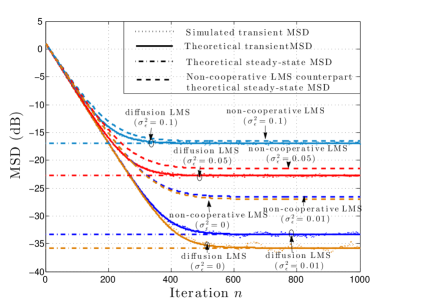
Refer to caption
Figure 4: Network MSD behavior for the perturbation-only case. Theoretical MSD curves were obtained by Corollary 1 and steady-state MSD values were obtained by Corollary 2. Note that simulated and theoretical transient MSD curves are superimposed.

V-A3 Correlated in time inputs

This simulation example illustrates the accuracy of models (62)–(67) for inputs correlated in time. We considered regression vectors

𝒙k(n)=[xk(n)xk(n1)]subscript𝒙𝑘𝑛superscriptdelimited-[]subscript𝑥𝑘𝑛subscript𝑥𝑘𝑛1top\boldsymbol{x}_{k}(n)=[x_{k}(n)\;x_{k}(n-1)]^{\top} (105)

with a first-order AR model given by

xk(n)=0.5xk(n1)+(10.52)σx,k2wk(n).subscript𝑥𝑘𝑛0.5subscript𝑥𝑘𝑛11superscript0.52superscriptsubscript𝜎𝑥𝑘2subscript𝑤𝑘𝑛x_{k}(n)=0.5\,x_{k}(n-1)+\sqrt{(1-0.5^{2})\sigma_{x,k}^{2}}\,w_{k}(n). (106)

The parameters σx,k2subscriptsuperscript𝜎2𝑥𝑘\sigma^{2}_{x,k} were set as in Fig. 1(b). The noise wk(n)subscript𝑤𝑘𝑛w_{k}(n) was i.i.d. and drawn from a zero-mean Gaussian distribution with variance σw2=1superscriptsubscript𝜎𝑤21\sigma_{w}^{2}=1, so that

𝑹x,k=σx,k2(10.50.51)subscript𝑹𝑥𝑘superscriptsubscript𝜎𝑥𝑘210.50.51\boldsymbol{R}_{x,k}=\sigma_{x,k}^{2}\left(\begin{array}[]{cc}1&0.5\\ 0.5&1\end{array}\right)

The diffusion LMS algorithm was tested in the following experimental settings:

𝒮1:{r=0.01,σϵ=0.010}𝒮2:{r=0.05,σϵ=0.015}𝒮3:{r=0.10,σϵ=0.015}.:subscript𝒮1formulae-sequence𝑟0.01subscript𝜎italic-ϵ0.010subscript𝒮2:formulae-sequence𝑟0.05subscript𝜎italic-ϵ0.015subscript𝒮3:formulae-sequence𝑟0.10subscript𝜎italic-ϵ0.015\begin{split}{{\mathcal{S}}}_{1}&:\{r=0.01,\sigma_{\epsilon}=0.010\}\\ {{\mathcal{S}}}_{2}&:\{r=0.05,\sigma_{\epsilon}=0.015\}\\ {{\mathcal{S}}}_{3}&:\{r=0.10,\sigma_{\epsilon}=0.015\}.\end{split} (107)

Although Assumption 1 is not valid, observe in Fig. 5 that the theoretical and simulated transient MSD curves are superimposed. This illustrates the accuracy of the analysis when the step-sizes are sufficiently small.
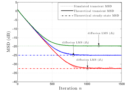
Refer to caption
Figure 5: Network MSD behavior for correlated inputs. Theoretical MSD curves were obtained by Corollary 1 and steady-state MSD values were obtained by Corollary 2. Simulated curves and theoretical curves are accurately superimposed.

V-B Adaptive clustering in multitask networks

We shall now illustrate the performance of diffusion LMS with adaptive clustering in a multitask environment. Our approach is compared with the strategy introduced in [43]. For the latter, as suggested in [43], the so-called smoothing factor γ𝛾\gamma was set to 0.10.10.1. A stationary problem is first considered. Next, a dynamic problem with time-varying clusters is introduced in order to confirm the reliability of our approach.

V-B1 Stationary environment

Consider the network of 161616 agents depicted in Fig. 6(a). The regression inputs 𝒙k(n)subscript𝒙𝑘𝑛\boldsymbol{x}_{k}(n) were zero-mean 2×1212\times 1 random vectors governed by a Gaussian distribution with covariance matrices 𝑹x,k=σx,k2𝑰Lsubscript𝑹𝑥𝑘superscriptsubscript𝜎𝑥𝑘2subscript𝑰𝐿\boldsymbol{R}_{x,k}=\sigma_{x,k}^{2}\,\boldsymbol{I}_{L}. The background noises zk(n)subscript𝑧𝑘𝑛z_{k}(n) were i.i.d. zero-mean Gaussian random variables, independent of any other signals. The variances σx,k2superscriptsubscript𝜎𝑥𝑘2\sigma_{x,k}^{2} and σz,k2superscriptsubscript𝜎𝑧𝑘2\sigma_{z,k}^{2} are depicted in Fig. 6(b). The scenario under study is a multitask problem with a cluster structure. Nodes 111 to 444 belong to the first cluster. Nodes 555 to 999 are in the second cluster. Nodes 101010 to 141414 compose the third cluster, and nodes 151515 and 161616 are in the fourth cluster. The parameter vectors to be estimated are as follows:

𝒘k={[0.50.4]k=1,,4Cluster 1[0.60.2]k=5,,9Cluster 2[0.30.3]k=10,,14Cluster 3[0.8  0.5]k=15,16Cluster 4superscriptsubscript𝒘𝑘casesmissing-subexpressionsuperscriptdelimited-[]0.50.4top𝑘14Cluster 1missing-subexpressionsuperscriptdelimited-[]0.60.2top𝑘59Cluster 2missing-subexpressionsuperscriptdelimited-[]0.30.3top𝑘1014Cluster 3missing-subexpressionsuperscriptdelimited-[]0.80.5top𝑘1516Cluster 4\boldsymbol{w}_{k}^{\star}=\left\{\begin{array}[]{lllr}&[0.5\,-0.4]^{\top}&k=1,\dots,4&\quad\text{Cluster 1}\\ &[0.6\,-0.2]^{\top}&k=5,\dots,9&\quad\text{Cluster 2}\\ &[0.3\,-0.3]^{\top}&k=10,\dots,14&\quad\text{Cluster 3}\\ &[-0.8\;\;0.5]^{\top}&k=15,16&\quad\text{Cluster 4}\end{array}\right. (108)

Note that the distances between the optimum parameter vectors for clusters 1, 2 and 3 are much smaller than those with respect to cluster 4, which acts as an outlier. The following algorithms were considered for estimating the four optimum parameter vectors: 1) diffusion LMS with a uniform combination matrix 𝑨𝑨\boldsymbol{A}, 2) non-cooperative LMS, 3) diffusion LMS with the clustering strategy introduced in [43], 4) diffusion LMS with our clustering strategy, with 𝑪=𝑰𝑪𝑰\boldsymbol{C}=\boldsymbol{I} and 𝑪(n)=𝑨(n)𝑪𝑛superscript𝑨top𝑛\boldsymbol{C}(n)=\boldsymbol{A}^{\top}(n). The step-size was set to μ=0.01𝜇0.01\mu=0.01 for all nodes.

Refer to caption
(a) Network topology
Refer to caption
(b) Input variances (top) and noise variances (bottom)
Figure 6: Network topology in Section V-B1 and associated input variances and noise variances.

Figure 7(a) illustrates the MSD convergence behavior for these algorithms. Due to large bias of the estimated weights, diffusion LMS with a uniform combination matrix had large MSD. Non-cooperative LMS performed much better as it provides unbiased estimates. The proposed algorithm with 𝑪=𝑰𝑪𝑰\boldsymbol{C}=\boldsymbol{I} achieved better performance, and 𝑪(n)=𝑨(n)𝑪𝑛superscript𝑨top𝑛\boldsymbol{C}(n)=\boldsymbol{A}^{\top}(n) led to additional performance gain due to information exchange. Finally, in order to provide a straightforward but visually-meaningful clustering result, we averaged the combination matrix 𝑨𝑨\boldsymbol{A} over the last 100 iterations of a single realization, and we considered that ak>0.05subscript𝑎𝑘0.05a_{\ell k}>0.05 represents a one-way connection from \ell to k𝑘k. The estimated relationships between nodes provided in Fig. 7(b) perfectly match the ground truth configuration.
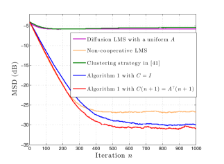
Refer to caption
(a) MSD behavior.
Refer to caption
(b) Estimated cluster structure.
Figure 7: Network MSD comparison in a stationary multitask environment, and estimated cluster structure by the proposed algorithm (averaged over the last 100 instants in one realization). The weight iterates for [43] were initialized at the same value. If random well-separated initial conditions are used across the nodes, then the performance of [43] becomes similar to that of the non-cooperative solution in the above plot.

V-B2 Non-stationary environment

Consider now a more complex environment where clusters vary over time. Four stationary stages and three transient episodes were modeled in this experiment. Properties of input signals and noise were the same as those in the stationary case considered above. From instant n=1𝑛1n=1 to 100010001000, the network consisted of one cluster with a unique optimum parameter vector to estimate. From n=1501𝑛1501n=1501 to 250025002500, nodes were split into two clusters with two different optimums. From n=3001𝑛3001n=3001 to 400040004000, nodes were split again to give four clusters. Finally, from instant n=4501𝑛4501n=4501, nodes were aggregated into one cluster with another unique parameter vector to estimate. Transient episodes were designed with linear interpolation between each steady-state stage over a period of 500500500 time samples. Taking, for example, the first component of the weight vector of node 111 over the time interval 111 to 250025002500, the time-variant optimum w1,1(n)superscriptsubscript𝑤11𝑛w_{1,1}^{\star}(n) is expressed by

w1,1(n)={0.3,n=1,,10000.3+0.50.3500(n1000),n=1001,,15000.5,n=1501,,2500.superscriptsubscript𝑤11𝑛cases0.3𝑛110000.30.50.3500𝑛1000𝑛100115000.5𝑛15012500w_{1,1}^{\star}(n)\!=\!\left\{\begin{array}[]{ll}0.3,&n=1,\dots,1000\\ 0.3+\frac{0.5-0.3}{500}(n-1000),&n=1001,\dots,1500\\ 0.5,&n=1501,\dots,2500.\end{array}\right. (109)

Cluster structures and optimum parameter vectors are illustrated in Fig. 8 and 9, respectively.

The same four algorithms as before were considered for comparison. Figure 10 shows their mean weight behavior. Conventional diffusion LMS with a uniform combination matrix made all nodes converge to the same Pareto optimum during all phases. The non-cooperative LMS estimated the optimum weight vectors without bias. The algorithm presented in [43], which generally performs well for well-separated tasks and well-separated initial random weights, did not perform well with this setting. Our algorithm showed the same convergence behavior for 𝑪=𝑰𝑪𝑰\boldsymbol{C}=\boldsymbol{I} and 𝑪(n)=𝑨(n)𝑪𝑛superscript𝑨top𝑛\boldsymbol{C}(n)=\boldsymbol{A}^{\top}(n). Only the case 𝑪(n)=𝑨(n)𝑪𝑛superscript𝑨top𝑛\boldsymbol{C}(n)=\boldsymbol{A}^{\top}(n) is presented here due to space limitation. It can be observed that, for each node, the parameter vector converged properly in accordance to the original cluster structures represented in Fig. 8. MSD learning curves are shown in Fig. 11. Transient stages can be clearly observed on both weight behavior and MSD behavior curves. Diffusion LMS enforced the weight vectors estimated by each agent to converge to the same solution at each stage. As a consequence, the MSD learning curve shows poor performance due to large bias. Non-cooperative LMS converged without bias towards the optimum parameter vectors. The algorithm introduced by [43] showed some ability to conduct clustering but did not provide satisfactory results during transient episodes. During stages 1 and 4, it worked as well as diffusion LMS. However, during stages 2 and 3, it only performed slightly better than diffusion LMS. The proposed algorithm was able to track the system dynamic with correct clustering and appropriate convergence in the mean-square sense.
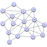
Refer to captionRefer to caption
Refer to caption
Figure 8: Evolution of cluster structures of the network (1 cluster \rightarrow 2 clusters \rightarrow 4 clusters \rightarrow 1 cluster).
Refer to caption
Figure 9: Evolution of clusters over time. Colors are consistent with those of clusters in Fig. 8. Dashed lines represent optimums during transient episodes.
Refer to caption
(a) Diffusion LMS with uniform 𝑨𝑨\boldsymbol{A}, 𝑪𝑪\boldsymbol{C}.
Refer to caption
(b) Non-cooperative LMS.
Refer to caption
(c) Algorithm in [43].
Refer to caption
(d) Proposed with 𝑪(n)=𝑨(n)𝑪𝑛superscript𝑨top𝑛\boldsymbol{C}(n)=\boldsymbol{A}^{\top}\!(n).
Figure 10: Mean weight behavior of various algorithms in the non-stationary environment. Colors are consistent with cluster colors in Fig. 6(a).

Refer to caption

Figure 11: Network MSD behavior comparison in the time variant multitask environment.

V-B3 Large network and high-dimensional regressors

For the sake of simplicity, previous experiments were conducted with relatively small networks and low-dimensional optimum parameter vectors. A network consisting of two clusters with 505050 nodes in each cluster was randomly deployed in a given area, with physical connections defined by the connectivity matrix in Fig. 12(b). The optimum parameter vectors were set as follows: 𝒘k=𝟏50subscriptsuperscript𝒘𝑘subscript150\boldsymbol{w}^{\star}_{k}={\boldsymbol{1}}_{50} for k=1,,50𝑘150k=1,\dots,50, and 𝒘k=𝟏50subscriptsuperscript𝒘𝑘subscript150\boldsymbol{w}^{\star}_{k}=-{\boldsymbol{1}}_{50} for k=51,,100𝑘51100k=51,\dots,100. The regression inputs 𝒙k(n)subscript𝒙𝑘𝑛\boldsymbol{x}_{k}(n) were zero-mean 50×150150\times 1 random vectors governed by a Gaussian distribution with covariance matrices 𝑹x,k=σx,k2𝑰Lsubscript𝑹𝑥𝑘superscriptsubscript𝜎𝑥𝑘2subscript𝑰𝐿\boldsymbol{R}_{x,k}=\sigma_{x,k}^{2}\,\boldsymbol{I}_{L}. The background noises zk(n)subscript𝑧𝑘𝑛z_{k}(n) were i.i.d. zero-mean Gaussian random variables, and independent of any other signal. The variances σx,k2superscriptsubscript𝜎𝑥𝑘2\sigma_{x,k}^{2} and σz,k2superscriptsubscript𝜎𝑧𝑘2\sigma_{z,k}^{2} were uniformly sampled in [0.8,1.2]0.81.2[0.8,1.2] and [0.018,0.022]0.0180.022[0.018,0.022], respectively. For all nodes, the step-sizes were set to μk=0.01subscript𝜇𝑘0.01\mu_{k}=0.01. The same four algorithms as before were considered. Our algorithm was used with the normalized gradient 𝒒k(n)/(𝒒k(n)+ξ)subscript𝒒𝑘𝑛normsubscript𝒒𝑘𝑛𝜉{\boldsymbol{q}}_{k}(n)/(\|{\boldsymbol{q}}_{k}(n)\|+\xi) and ξ=0.01𝜉0.01\xi=0.01. MSD learning curves are shown in Fig. 12(a), and the connectivity matrix determined by our algorithm is represented in Fig. 12(c). It can be observed that the performance of our algorithm is better than that of other methods.
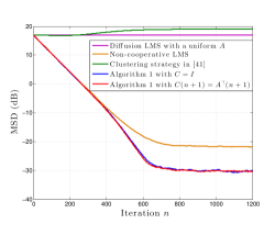
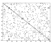
Refer to caption
(a) MSD learning curves.
Refer to caption
(b) Network physical connection matrix.
Refer to caption
(c) Connection selected by the algorithm.
Figure 12: Simulation results on a large network (N=100𝑁100N=100) with high-dimensional regressors (L=50)𝐿50(L=50). (a) Comparison of MSD learning curves. (b) Initial connectivity matrix, where gray elements represent physical connections. (c) Connectivity matrix resulting from our clustering strategy.

V-C Collaborative target tracking over sensor networks

Consider now a target tracking problem to illustrate our adaptive clustering strategy with diffusion LMS. We focused on a scenario involving four targets, numbered from i=1𝑖1i=1 to 444, moving according to the state-transition equation

𝒙i(n+1)=𝑻i𝒙i(n)+𝒛i(n)for i=1,,4,n=0,,100\begin{split}&\boldsymbol{x}_{i}(n+1)=\boldsymbol{T}^{\star}_{i}\;\boldsymbol{x}_{i}(n)+{\boldsymbol{z}}_{i}(n)\\ &\text{for }\;i=1,\dots,4,\quad n=0,\dots,100\end{split} (110)

where 𝒙i(n)subscript𝒙𝑖𝑛\boldsymbol{x}_{i}(n) is the 2-dimensional coordinates for target i𝑖i at instant n𝑛n. Matrices 𝑻isubscript𝑻𝑖\boldsymbol{T}_{i} are 2×2222\times 2 state-transition matrices that were set to

𝑻1=(1.00190.01290.01871.0034),𝑻2=(1.01490.00140.00331.0034),𝑻3=(1.01280.00410.01561.0086),𝑻4=𝑻1formulae-sequencesubscriptsuperscript𝑻11.00190.01290.01871.0034formulae-sequencesubscriptsuperscript𝑻21.01490.00140.00331.0034formulae-sequencesubscriptsuperscript𝑻31.01280.00410.01561.0086subscriptsuperscript𝑻4subscriptsuperscript𝑻1\begin{split}&\boldsymbol{T}^{\star}_{1}\!=\!\left(\begin{array}[]{cc}1.0019&-0.0129\\ 0.0187&\phantom{-}1.0034\end{array}\right),\,\boldsymbol{T}^{\star}_{2}\!=\!\left(\begin{array}[]{cc}1.0149&-0.0014\\ 0.0033&\phantom{-}1.0034\end{array}\right),\\ &\boldsymbol{T}^{\star}_{3}\!=\!\left(\begin{array}[]{cc}1.0128&-0.0041\\ 0.0156&\phantom{-}1.0086\end{array}\right),\,\boldsymbol{T}^{\star}_{4}\!=\!\boldsymbol{T}^{\star}_{1}\end{split} (111)

and 𝒛i(n)subscript𝒛𝑖𝑛{\boldsymbol{z}}_{i}(n) is the modeling error with i.i.d. zero-mean Gaussian distribution with covariance matrix σz2𝑰superscriptsubscript𝜎𝑧2𝑰\sigma_{z}^{2}\,\boldsymbol{I}. The standard deviation was set to σz=0.01subscript𝜎𝑧0.01\sigma_{z}=0.01. The initial coordinates for the four targets were

𝒙1(0)=𝒙2(0)=𝒙3(0)=[11],𝒙4(0)=[1.21.2].formulae-sequencesubscript𝒙10subscript𝒙20subscript𝒙30superscriptdelimited-[]11topsubscript𝒙40superscriptdelimited-[]1.21.2top\boldsymbol{x}_{1}(0)=\boldsymbol{x}_{2}(0)=\boldsymbol{x}_{3}(0)=[1\,-1]^{\top},\quad\boldsymbol{x}_{4}(0)=[1.2\,-1.2]^{\top}. (112)

Figure 13(a) shows the trajectories of the four targets from instant n=0𝑛0n=0 to 100100100. A network with N=100𝑁100N=100 nodes was randomly deployed in a given area, with physical connections defined by the connectivity matrix in Fig. 14(a).

We supposed that each node was able to track only one target during the experiment, with noisy observations 𝒙~k(n)subscript~𝒙𝑘𝑛\tilde{\boldsymbol{x}}_{k}(n):

𝒙~k(n)=𝒙k(n)+𝒖k(n)for k=1,,Nformulae-sequencesubscript~𝒙𝑘𝑛subscript𝒙𝑘𝑛subscript𝒖𝑘𝑛for 𝑘1𝑁\tilde{\boldsymbol{x}}_{k}(n)=\boldsymbol{x}_{k}(n)+\boldsymbol{u}_{k}(n)\qquad\text{for }\;k=1,\dots,N (113)

with 𝒖k(n)subscript𝒖𝑘𝑛\boldsymbol{u}_{k}(n) an i.i.d. zero-mean Gaussian observation noise with covariance matrix σu2𝑰superscriptsubscript𝜎𝑢2𝑰\sigma_{u}^{2}\boldsymbol{I} and standard deviation σu=0.01subscript𝜎𝑢0.01\sigma_{u}=0.01. For ease of presentation, we assumed that nodes 111252525 tracked target 111, nodes 262626505050 tracked target 222, nodes 515151757575 tracked target 333, and nodes 767676100100100 tracked target 444.

Considering 𝒙~(n)~𝒙𝑛\tilde{\boldsymbol{x}}(n) as input data and 𝒙~(n+1)~𝒙𝑛1\tilde{\boldsymbol{x}}(n+1) as the desired output data for the learning algorithm, each node was aimed to track a target or, equivalently, to estimate its transition matrix given input-output noisy data. Without cooperation, this task can be performed by each node k𝑘k by minimizing the following cost function with respect to matrix 𝑻ksubscript𝑻𝑘\boldsymbol{T}_{k}:

Jk(𝑻k)=𝔼𝒙~k(n+1)𝑻k𝒙~k(n)2for k=1,,N.formulae-sequencesubscript𝐽𝑘subscript𝑻𝑘𝔼superscriptnormsubscript~𝒙𝑘𝑛1subscript𝑻𝑘subscript~𝒙𝑘𝑛2for 𝑘1𝑁J_{k}({\boldsymbol{T}_{k}})=\mathbb{E}\|\tilde{\boldsymbol{x}}_{k}(n+1)-{\boldsymbol{T}_{k}}\,\tilde{\boldsymbol{x}}_{k}(n)\|^{2}\qquad\text{for }k=1,\dots,N. (114)

Collaboration among nodes may be beneficial as several nodes are conducting the same task, including nodes that track the same target and nodes that track distinct targets with the same state-transition matrix. Clearly, diffusion LMS with a uniform combination matrix is not suitable within this context since neighboring nodes may not have the same task to conduct. This problem requires adaptive clustering to automatically aggregate nodes that perform a similar task.

Algorithm 1 was run with 𝑪=𝑰N𝑪subscript𝑰𝑁\boldsymbol{C}=\boldsymbol{I}_{N} and was initialized with 𝑻k(0)=𝑰2subscript𝑻𝑘0subscript𝑰2\boldsymbol{T}_{k}(0)=\boldsymbol{I}_{2}. The step-size μ𝜇\mu was set equal to μ=0.05𝜇0.05\mu=0.05. Figure 13(b) shows the MSD learning curves of transition matrices estimated by non-cooperative LMS, and diffusion LMS with adaptive clustering strategy. The performance gain can be clearly seen from these figures. Figure 14(b) shows the connectivity matrix determined by the clustering strategy at iteration n=100𝑛100n=100. Gray elements in this figure represent the combination weights aksubscript𝑎𝑘a_{\ell k} that are larger than 0.050.050.05. It can be seen that connections are distributed in 444 blocks on the diagonal, each one corresponding to a target, and 2 other blocks (upper-right and lower-left ones) where nodes track two distinct targets with the same state-transition matrix.
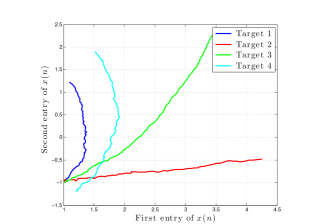
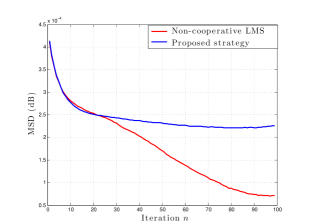
Refer to caption
(a) Target trajectories.
Refer to caption
(b) MSD learning curves.
Figure 13: (a) Trajectories of four targets with initial coordinates 𝐱1(0)=𝐱2(0)=𝐱3(0)=[1,1],𝐱4(0)=[1.2,1.2]formulae-sequencesubscript𝐱10subscript𝐱20subscript𝐱30superscript11topsubscript𝐱40superscript1.21.2top\boldsymbol{x}_{1}(0)=\boldsymbol{x}_{2}(0)=\boldsymbol{x}_{3}(0)=[1,-1]^{\top},\boldsymbol{x}_{4}(0)=[1.2,-1.2]^{\top}, from n=0𝑛0n=0 to 100100100. (b) Comparison of MSD learning curves for the estimate 𝐓ksubscript𝐓𝑘\boldsymbol{T}_{k}.
Refer to caption
(a) Network physical connection matrix.
Refer to caption
(b) Connections selected collaboratively by the algorithm.
Figure 14: (a) Initial connectivity matrix, where gray elements represent physical connections. (b) Connectivity matrix resulting from our clustering strategy. Blue elements correspond to the connections used to estimate the transition matrices 𝐓1=𝐓4superscriptsubscript𝐓1superscriptsubscript𝐓4\boldsymbol{T}_{1}^{\star}=\boldsymbol{T}_{4}^{\star}. Red and green elements correspond to the connections used to estimate the transition matrices 𝐓2superscriptsubscript𝐓2\boldsymbol{T}_{2}^{\star} and 𝐓3superscriptsubscript𝐓3\boldsymbol{T}_{3}^{\star}, respectively. Gray elements can be considered as false connections because they involve nodes that do not estimate the same transition matrix.

VI Conclusion and perspectives

Many practical problems of interest happen to be multitask-oriented in the sense that there are multiple optimum parameter vectors to be inferred simultaneously. In this paper, we studied the performance of the single-task diffusion LMS algorithm when it is run in a multitask environment. Accurate mean weight behavior model and mean square deviation model were derived. Next, we proposed an unsupervised clustering strategy that allows each node to select the neighboring nodes with which it can collaborate to address a given task. Simulations were presented to demonstrate the efficiency of the proposed clustering strategy.

References

  • [1] J. Chen and C. Richard, “Performance analysis of diffusion LMS in multitask networks,” in Proc. IEEE Int. Workshop on Computational Advances in Multi-Sensor Adaptive Processing (CAMSAP), Saint Martin, France, Dec. 2013, pp. 137–140.
  • [2] A. H. Sayed, “Adaptive networks,” Proc. of the IEEE, vol. 102, no. 4, pp. 460–497, Apr. 2014.
  • [3] J. Tsitsiklis and M. Athans, “Convergence and asymptotic agreement in distributed decision problems,” IEEE Trans. Autom. Control, vol. 29, no. 1, pp. 42–50, Jan. 1984.
  • [4] L. Xiao and S. Boyd, “Fast linear iterations for distributed averaging,” Syst. Control lett., vol. 53, no. 9, pp. 65–78, Sept. 2004.
  • [5] P. Braca, S. Marano, and V. Matta, “Enforcing consensus while monitoring the environment in wireless sensor networks,” IEEE Trans. Signal Process., vol. 56, no. 7, pp. 3375–3380, Jul. 2008.
  • [6] A. Nedic and A. Ozdaglar, “Distributed subgradient methods for multi-agent optimization,” IEEE Trans. Autom. Control, vol. 54, no. 1, pp. 48–61, Jan. 2009.
  • [7] S. Kar and J. M. F. Moura, “Distributed consensus algorithms in sensor networks: Link failures and channel noise,” IEEE Trans. Signal Process., vol. 57, no. 1, pp. 355–369, Jan. 2009.
  • [8] P. Braca, S. Marano, V. Matta, and P. Willett, “Asymptotic optimality of running consensus in testing binary hypotheses,” IEEE Trans. Signal Process., vol. 58, no. 2, pp. 814–825, Feb. 2010.
  • [9] A. G. Dimakis, S. Kar, J. M. F. Moura, M. G. Rabbat, and A. Scaglione, “Gossip algorithms for distributed signal processing,” Proc. of the IEEE, vol. 98, no. 11, pp. 1847–1864, Nov. 2010.
  • [10] K. Srivastava and A. Nedic, “Distributed asynchronous constrained stochastic optimization,” IEEE J. Sel. Topics Signal Process., vol. 5, no. 4, pp. 772–790, Aug. 2011.
  • [11] D. P. Bertsekas, “A new class of incremental gradient methods for least squares problems,” SIAM J. Optimiz., vol. 7, no. 4, pp. 913–926, Nov. 1997.
  • [12] A. Nedic and D. P. Bertsekas, “Incremental subgradient methods for nondifferentiable optimization,” SIAM J. Optimiz., vol. 12, no. 1, pp. 109–138, Jul. 2001.
  • [13] M. G. Rabbat and R. D. Nowak, “Quantized incremental algorithms for distributed optimization,” IEEE J. Sel. Areas Commun., vol. 23, no. 4, pp. 798–808, Apr. 2005.
  • [14] D. Blatt, A. O. Hero, and H. Gauchman, “A convergent incremental gradient method with constant step size,” SIAM J. Optimiz., vol. 18, no. 1, pp. 29–51, Feb. 2007.
  • [15] C. G. Lopes and A. H. Sayed, “Incremental adaptive strategies over distributed networks,” IEEE Trans. Signal Process., vol. 55, no. 8, pp. 4064–4077, Aug. 2007.
  • [16] C. G. Lopes and A. H. Sayed, “Diffusion least-mean squares over adaptive networks: Formulation and performance analysis,” IEEE Trans. Signal Process., vol. 56, no. 7, pp. 3122–3136, Jul. 2008.
  • [17] F. S. Cattivelli and A. H. Sayed, “Diffusion LMS strategies for distributed estimation,” IEEE Trans. Signal Process., vol. 58, no. 3, pp. 1035–1048, Mar. 2010.
  • [18] S.-Y. Tu and A. H. Sayed, “Diffusion strategies outperform consensus strategies for distributed estimation over adaptive netowrks,” IEEE Trans. Signal Process., vol. 60, no. 12, pp. 6217–6234, Dec. 2012.
  • [19] J. Chen and A. H. Sayed, “Diffusion adaptation strategies for distributed optimization and learning over networks,” IEEE Trans. Signal Process., vol. 60, no. 8, pp. 4289–4305, Aug. 2012.
  • [20] A. Khalili, M. A. Tinati, A. Rastegarnia, and J. A. Chambers, “Steady-state analysis of diffusion LMS adaptive networks with noisy links,” IEEE Trans. Signal Process., vol. 60, no. 2, pp. 974–979, Feb. 2012.
  • [21] X. Zhao, S.-Y. Tu, and A. H. Sayed, “Diffusion adaptation over networks under imperfect information exchange and non-stationary data,” IEEE Trans. Signal Process., vol. 60, no. 7, pp. 3460–3475, Jul. 2012.
  • [22] J. Chen and A. H. Sayed, “Distributed Pareto optimization via diffusion strategies,” IEEE J. Sel. Topics Signal Process., vol. 7, no. 2, pp. 205–220, Apr. 2013.
  • [23] O. N. Gharehshiran, V. Krishnamurthy, and G. Yin, “Distributed energy-aware diffusion least mean squares: Game-theoretic learning,” IEEE J. Sel. Topics Signal Process., vol. 7, no. 5, pp. 1–16, Oct. 2013.
  • [24] S. Chouvardas, K. Slavakis, and S. Theodoridis, “Adaptive robust distributed learning in diffusion sensor networks,” IEEE Trans. Signal Process., vol. 59, no. 10, pp. 4692–4707, Oct. 2011.
  • [25] A. H. Sayed, “Adaptation, learning, and optimization over networks,” in Foundations and Trends in Machine Learning, vol. 7, pp. 311–801. NOW Publishers, Boston-Delft, Jul. 2014.
  • [26] Y. Liu, C. Li, and Z. Zhang, “Diffusion sparse least-mean squares over networks,” IEEE Trans. Signal Process., vol. 60, no. 8, pp. 4480–4485, Aug. 2012.
  • [27] S. Chouvardas, K. Slavakis, Y. Kopsinis, and S. Theodoridis, “A sparsity-promoting adaptive algorithm for distributed learning,” IEEE Trans. Signal Process., vol. 60, no. 10, pp. 5412–5425, Oct. 2012.
  • [28] P. Di Lorenzo and A. H. Sayed, “Sparse distributed learning based on diffusion adaptation,” IEEE Trans. Signal Process., vol. 61, no. 6, pp. 1419–1433, Mar. 2013.
  • [29] P. Chainais and C. Richard, “Distributed dictionary learning over a sensor network,” in Proc. Conf. sur l’Apprentissage Automatique (CAP), Lille, France, Jul. 2013, pp. 1–6.
  • [30] P. Chainais and C. Richard, “Learning a common dictionary over a sensor network,” in Proc. IEEE Int. Workshop on Computational Advances in Multi-Sensor Adaptive Processing (CAMSAP), Saint Martin, France, Dec. 2013, pp. 1–4.
  • [31] J. Predd, S. Kulkarni, and H. Vincent Poor, “Distributed learning in wireless sensor networks,” IEEE Signal Process. Mag., vol. 23, no. 4, pp. 59–69, Jul. 2006.
  • [32] P. Honeine, M. Essoloh, C. Richard, and H. Snoussi, “Distributed regression in sensor networks with a reduced-order kernel model,” in Proc. IEEE Global Telecommun. Conf. (GLOBECOM), New Orleans, LO, USA, 2008, pp. 1–5.
  • [33] J. Chen, L. Tang, J. Liu, and J. Ye, “A convex formulation for leaning shared structures from muliple tasks,” in Proc. Ann. Int. Conf. Machine Learning (ICML), Montreal, Canada, Jun. 2009, pp. 137–144.
  • [34] O. Chapelle, P. Shivaswmy, K. Q. Vadrevu, S. Weinberger, Y. Zhang, and B. Tseng, “Multi-task learning for boosting with application to web search ranking,” in Proc. ACM SIGKDD int. Conf. Knowledge Discovery and Data Mining, Washington DC, USA, Jul. 2010, pp. 1189–1198.
  • [35] J. Zhou, L. Yuan, J. Liu, and J. Ye, “A multi-task learning formulation for predicting disease progression,” in Proc. ACM SIGKDD int. Conf. Knowledge Discovery and Data Mining, San Diego, CA, USA, Aug. 2011, pp. 814–822.
  • [36] J. Chen, C. Richard, and A. H. Sayed, “Multitask diffusion LMS over networks,” IEEE Trans. Signal Process., vol. 62, no. 16, pp. 4129–4144, Aug. 2014. Extended report available as arXiv: 1311.4894 [cs.MA], Nov. 2013.
  • [37] R. Abdolee, B. Champagne, and A. H. Sayed, “Estimation of space-time varying parameters using a diffusion LMS algorithm,” IEEE Trans. Signal Process., vol. 62, no. 2, pp. 403–418, Jan. 2014.
  • [38] A. Bertrand and M. Moonen, “Distributed adaptive node-specific signal estimation in fully connected sensor networks – Part I: sequential node updating,” IEEE Trans. Signal Process., vol. 58, no. 10, pp. 5277–5291, Oct. 2010.
  • [39] A. Bertrand and M. Moonen, “Distributed adaptive estimation of node-specific signals in wireless sensor networks with a tree topology,” IEEE Trans. Signal Process., vol. 59, no. 5, pp. 2196–2210, May 2011.
  • [40] N. Bogdanović, J. Plata-Chaves, and K. Berberidis, “Distributed incremental-based LMS for node-specific parameter estimation over adaptive networks,” in Proc. IEEE Int. Conf. Acoust., Speech, Signal Process., Vancouver, Canada, May 2013, pp. 5425–5429.
  • [41] N. Bogdanović, J. Plata-Chaves, and K. Berberidis, “Distributed diffusion-based LMS for node-specific parameter estimation over adaptive networks,” in Proc. IEEE Int. Conf. Acoust., Speech, Signal Process., Florence, Italy, May 2014, pp. 7223–7227.
  • [42] J. Chen, C. Richard, A. O. Hero, and A. H. Sayed, “Diffusion LMS for multitask problems with overlapping hypothesis subspaces,” in Proc. IEEE Int. Workshop on Machine Learn. for Signal Process., Reims, France, Sept. 2014, pp. 1–6.
  • [43] X. Zhao and A. H. Sayed, “Clustering via diffusion adaptation over networks,” in Proc. Int. Workshop Cognitive Inf. Process. (CIP), Parador de Baiona, Spain, May 2012, pp. 1–6.
  • [44] A. H. Sayed, “Diffusion adaptation over networks,” in Academic Press Libraray in Signal Processing, R. Chellapa and S. Theodoridis, Eds., pp. 322–454. Elsevier, 2014. Also available as arXiv:1205.4220 [cs.MA], May 2012.
  • [45] S. Boyd and L. Vandenberghe, Convex Optimization, Cambridge university press, 2004.
  • [46] A. H. Sayed, S.-Y Tu, J. Chen, X. Zhao, and Z. Towfic, “Diffusion strategies for adaptation and learning over networks,” IEEE Signal Process. Mag., vol. 30, no. 3, pp. 155–171, May 2013.
  • [47] A. H. Sayed, Adaptive Filters, John Wiley & Sons, NJ, 2008.
  • [48] K. M. Abadir and J. R. Magnus, Matrix Algebra, Cambridge Universiity Press, 2005.
  • [49] D. S. Bernstein, Matrix Mathematics: Theory, Facts, and Formulas, Princeton University Press, 2009.
Conversion to HTML had a Fatal error and exited abruptly. This document may be truncated or damaged.