SfePy - Write Your Own FE Application

Abstract

SfePy (Simple Finite Elements in Python) is a framework for solving various kinds of problems (mechanics, physics, biology, …) described by partial differential equations in two or three space dimensions by the finite element method. The paper illustrates its use in an interactive environment or as a framework for building custom finite-element based solvers.

1 Introduction

SfePy (Simple Finite Elements in Python) is a multi-platform (Linux, Mac OS X, Windows) software released under the New BSD license, see http://sfepy.org. It implements one of the standard ways of discretizing partial differential equations (PDEs) which is the finite element method (FEM) [R1].

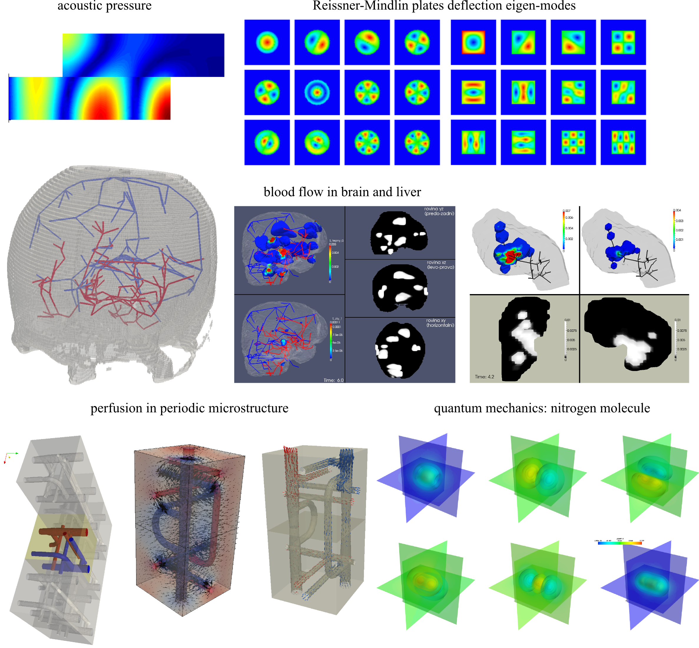
Figure 3: Gallery of applications. Perfusion and acoustic images by Vladimír Lukeš.

So far, SfePy has been employed for modelling in materials science, including, for example, multiscale biomechanical modelling (bone, muscle tissue with blood perfusion) [R2], [R3], [R4], [R5], [R6], [R7], computation of acoustic transmission coefficients across an interface of arbitrary microstructure geometry [R8], computation of phononic band gaps [R9], [R10], finite element formulation of Schroedinger equation [R11], and other applications, see also Figure 3. The software can be used as

• a collection of modules (a library) for building custom or domain-specific applications,

• a highly configurable "black box" PDE solver with problem description files in Python.

In this paper we focus on illustrating the former use by using a particular example. All examples presented below were tested to work with the version 2013.3 of SfePy.

2 Development

The SfePy project uses Git for source code management and GitHub web site for the source code hosting and developer interaction, similarly to many other scientific python tools. The version 2013.3 has been released in September 18. 2013, and its git-controlled sources contained 761 total files, 138191 total lines (725935 added, 587744 removed) and 3857 commits done by 15 authors. However, about 90% of all commits were done by the main developer as most authors contributed only a few commits. The project seeks and encourages more regular contributors, see http://sfepy.org/doc-devel/development.html.

3 Short Description

The code is written mostly in Python. For speed in general, it relies on fast vectorized operations provided by NumPy [R12] arrays, with heavy use of advanced broadcasting and "index tricks" features. C and Cython [R13] are used in places where vectorization is not possible, or is too difficult/unreadable. Other components of the scientific Python software stack are used as well, among others: SciPy [R14] solvers and algorithms, Matplotlib [R15] for 2D plots, Mayavi [R16] for 3D plots and simple postprocessing GUI, IPython [R17] for a customized shell, SymPy [R18] for symbolic operations/code generation etc.

The basic structure of the code allows a flexible definition of various problems. The problems are defined using components directly corresponding to mathematical counterparts present in a weak formulation of a problem in the finite element setting: a solution domain and its sub-domains (regions), variables belonging to suitable discrete function spaces, equations as sums of terms (weak form integrals), various kinds of boundary conditions, material/constitutive parameters etc.

The key notion in SfePy is a term, which is the smallest unit that can be used to build equations (linear combinations of terms). It corresponds to a weak formulation integral and takes usually several arguments: (optional) material parameters, a single virtual (or test) function variable and zero or more state (or unknown) variables. The available terms (currently 105) are listed at our web site (http://sfepy.org/doc-devel/terms_overview.html). The already existing terms allow to solve problems from many scientific domains, see Figure 3. Those terms cover many common PDEs in continuum mechanics, poromechanics, biomechanics etc. with a notable exception of electromagnetism (work in progress, see below).

SfePy discretizes PDEs using a continuous Galerkin approximation with finite elements as defined in [R1]. Discontinuous element-wise constant approximation is also possible. Currently the code supports the 2D area (triangle, rectangle) and 3D volume (tetrahedron, hexahedron) elements. Structural elements like shells, plates, membranes or beams are not supported with a single exception of a hyperelastic Mooney-Rivlin membrane.

Several kinds of basis or shape functions can be used for the finite element approximation of the physical fields:

• the classical nodal (Lagrange) basis can be used with all element types;

• the hierarchical (Lobatto) basis can be used with tensor-product elements (rectangle, hexahedron).

Although the code can provide the basis function polynomials of a high order (10 or more), orders greater than 4 are not practically usable, especially in 3D. This is caused by the way the code assembles the element contributions into the global matrix - it relies on NumPy vectorization and evaluates the element matrices all at once and then adds to the global matrix - this allows fast term evaluation and assembling but its drawback is a very high memory consumption for high polynomial orders. Also, the polynomial order has to be uniform over the whole (sub)domain where a field is defined. Related to polynomial orders, tables with quadrature points for numerical integration are available or can be generated as needed.

We are now working on implementing Nédélec and Raviart-Thomas vector bases in order to support other kinds of PDEs, such as the Maxwell equations of electromagnetism.

Once the equations are assembled, a number solvers can be used to solve the problem. SfePy provides a unified interface to many standard codes, for example UMFPACK [R19], PETSc [R20], Pysparse [R21] as well as the solvers available in SciPy. Various solver classes are supported: linear, nonlinear, eigenvalue, optimization, and time stepping.

Besides the external solvers mentioned above, several solvers are implemented directly in SfePy.

Nonlinear/optimization solvers:

• The Newton solver with a backtracking line-search is the default solver for all problems. For simplicity we use a unified approach to solve both the linear and non-linear problems - former (should) converge in a single nonlinear solver iteration.

• The steepest descent optimization solver with a backtracking line-search can be used as a fallback optimization solver when more sophisticated solvers fail.

Time-stepping-related solvers:

• The stationary solver is used to solve time-independent problems.

• The equation sequence solver is a stationary solver that analyzes the dependencies among equations and solves smaller blocks first. An example would be the thermoelasticity problem described below, where the elasticity equation depends on the load given by temperature distribution, but the temperature distribution (Poisson equation) does not depend on deformation. Then the temperature distribution can be found first, followed by the elasticity problem with the already known temperature load. This greatly reduces memory usage and improves speed of solution.

• The simple implicit time stepping solver is used for (quasistatic) time-dependent problems, using a fixed time step.

• The adaptive implicit time stepping solver can change the time step according to a user provided function. The default function adapt_time_step() decreases the step in case of bad Newton convergence and increases the step (up to a limit) when the convergence is fast. It is convenient for large deformation (hyperelasticity) problems.

• The explicit time stepping solver can be used for dynamic problems.

4 Thermoelasticity Example

This example involves calculating a temperature distribution in an object followed by an elastic deformation analysis of the object loaded by the thermal expansion and boundary displacement constraints. It shows how to use SfePy in a script/interactively. The actual equations (weak form) are described below. The entire script consists of the following steps:

Import modules. The SfePy package is organized into several sub-packages. The example uses:

• sfepy.fem: the finite element method (FEM) modules

• sfepy.terms: the weak formulation terms - equations building blocks

• sfepy.solvers: interfaces to various solvers (SciPy, PETSc, …)

• sfepy.postprocess: post-processing & visualization based on Mayavi

import numpy as npfrom sfepy.fem import (Mesh, Domain, Field,                       FieldVariable,                       Material, Integral,                       Equation, Equations,                       ProblemDefinition)from sfepy.terms import Termfrom sfepy.fem.conditions import Conditions, EssentialBCfrom sfepy.solvers.ls import ScipyDirectfrom sfepy.solvers.nls import Newtonfrom sfepy.postprocess import ViewerLoad a mesh file defining the object geometry.

mesh = Mesh.from_file(’meshes/2d/square_tri2.mesh’)domain = Domain(’domain’, mesh)Define solution and boundary conditions domains, called regions.

omega = domain.create_region(’Omega’, ’all’)left = domain.create_region(’Left’,                            ’vertices in x < -0.999’,                            ’facet’)right = domain.create_region(’Right’,                             ’vertices in x > 0.999’,                             ’facet’)bottom = domain.create_region(’Bottom’,                              ’vertices in y < -0.999’,                              ’facet’)top = domain.create_region(’Top’,                           ’vertices in y > 0.999’,                           ’facet’)Save regions for visualization.

domain.save_regions_as_groups(’regions.vtk’)Use a quadratic approximation for temperature field, define unknown $T$ and test $s$ variables.

field_t = Field.from_args(’temperature’, np.float64,                          ’scalar’, omega, 2)t = FieldVariable(’t’, ’unknown’, field_t, 1)s = FieldVariable(’s’, ’test’, field_t, 1,                  primary_var_name=’t’)Define numerical quadrature for the approximate integration rule.

integral = Integral(’i’, order=2)Define the Laplace equation governing the temperature distribution:

$$\int_{\Omega}\nabla s\cdot\nabla T=0\;,\quad\forall s\;.$$

term = Term.new(’dw_laplace(s, t)’, integral, omega,                s=s, t=t)eq = Equation(’temperature’, term)eqs = Equations([eq])Set boundary conditions for the temperature: $T=10\mbox{ on }\Gamma_{\rm left}$, $T=30\mbox{ on }\Gamma_{\rm right}$.

t_left = EssentialBC(’t_left’,                     left, {’t.0’ : 10.0})t_right = EssentialBC(’t_right’,                      right, {’t.0’ : 30.0})Create linear (ScipyDirect) and nonlinear solvers (Newton).

ls = ScipyDirect({})nls = Newton({}, lin_solver=ls)Combine the equations, boundary conditions and solvers to form a full problem definition.

pb = ProblemDefinition(’temperature’, equations=eqs,                       nls=nls, ls=ls)pb.time_update(ebcs=Conditions([t_left, t_right]))Solve the temperature distribution problem to get $T$.

temperature = pb.solve()out = temperature.create_output_dict()Use a linear approximation for displacement field, define unknown $\underline{u}$ and test $\underline{v}$ variables. The variables are vectors with two components in any point, as we are solving on a 2D domain.

field_u = Field.from_args(’displacement’, np.float64,                          ’vector’, omega, 1)u = FieldVariable(’u’, ’unknown’, field_u, mesh.dim)v = FieldVariable(’v’, ’test’, field_u, mesh.dim,                  primary_var_name=’u’)Set Lamé parameters of elasticity $\lambda$, $\mu$, thermal expansion coefficient $\alpha_{ij}$ and background temperature $T_{0}$. Constant values are used here. In general, material parameters can be given as functions of space and time.

lam = 10.0 # Lame parameters.mu = 5.0te = 0.5 # Thermal expansion coefficient.T0 = 20.0 # Background temperature.eye_sym = np.array([[1], [1], [0]],                   dtype=np.float64)m = Material(’m’, lam=lam, mu=mu,             alpha=te * eye_sym)Define and set the temperature load variable to $T-T_{0}$.

t2 = FieldVariable(’t’, ’parameter’, field_t, 1,                   primary_var_name=’(set-to-None)’)t2.set_data(t() - T0)Define the thermoelasticity equation governing structure deformation:

$$\int_{\Omega}D_{ijkl}\ e_{ij}(\underline{v})e_{kl}(\underline{u})-\int_{\Omega}(T-T_{0})\ \alpha_{ij}e_{ij}(\underline{v})=0\;,\quad\forall\underline{v}\;,$$

where $D_{ijkl}=\mu(\delta_{ik}\delta_{jl}+\delta_{il}\delta_{jk})+\lambda\ \delta_{ij}\delta_{kl}$ is the homogeneous isotropic elasticity tensor and $e_{ij}(\underline{u})=\frac{1}{2}(\frac{\partial u_{i}}{\partial x_{j}}+\frac{\partial u_{j}}{\partial x_{i}})$ is the small strain tensor. The equations can be built as linear combinations of terms.

term1 = Term.new(’dw_lin_elastic_iso(m.lam, m.mu, v, u)’,                 integral, omega, m=m, v=v, u=u)term2 = Term.new(’dw_biot(m.alpha, v, t)’,                 integral, omega, m=m, v=v, t=t2)eq = Equation(’temperature’, term1 - term2)eqs = Equations([eq])Set boundary conditions for the displacements: $\underline{u}=0\mbox{ on }\Gamma_{\rm bottom}$, $u_{1}=0.0\mbox{ on }\Gamma_{\rm top}$ ($x$ -component).

u_bottom = EssentialBC(’u_bottom’,                       bottom, {’u.all’ : 0.0})u_top = EssentialBC(’u_top’,                    top, {’u.[0]’ : 0.0})Set the thermoelasticity equations and boundary conditions to the problem definition.

pb.set_equations_instance(eqs, keep_solvers=True)pb.time_update(ebcs=Conditions([u_bottom, u_top]))Solve the thermoelasticity problem to get $\underline{u}$.

displacement = pb.solve()out.update(displacement.create_output_dict())Save the solution of both problems into a single VTK file.

pb.save_state(’thermoelasticity.vtk’, out=out)Display the solution using Mayavi.

view = Viewer(’thermoelasticity.vtk’)view(vector_mode=’warp_norm’,     rel_scaling=1, is_scalar_bar=True,     is_wireframe=True,     opacity={’wireframe’ : 0.1})

4.1 Results

The above script saves the domain geometry as well as the temperature and displacement fields into a VTK file called ’thermoelasticity.vtk’ and also displays the results using Mayavi. The results are shown in Figures 1 and 2.

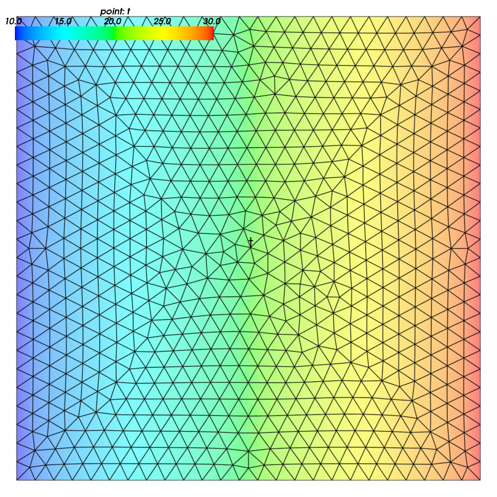
Figure 1: The temperature distribution.

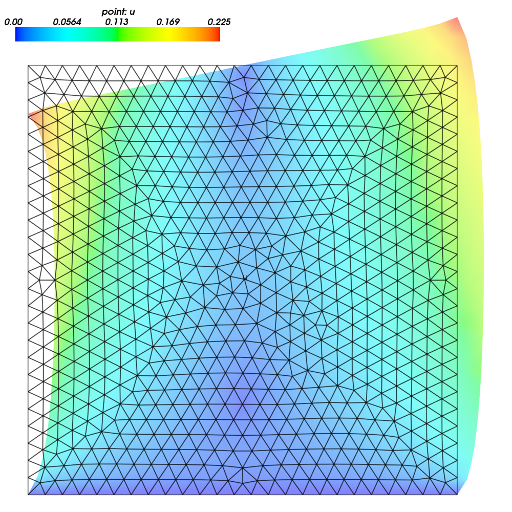
Figure 2: The deformed mesh showing displacements.

5 Alternative Way: Problem Description Files

Problem description files (PDF) are Python modules containing definitions of the various components (mesh, regions, fields, equations, …) using basic data types such as dict and tuple. For simple problems, no programming at all is required. On the other hand, all the power of Python (and supporting SfePy modules) is available when needed. The definitions are used to construct and initialize in an automatic way the corresponding objects, similarly to what was presented in the example above, and the problem is solved. The main script for running a simulation described in a PDF is called simple.py.

5.1 Example: Temperature Distribution

This example defines the problem of temperature distribution on a 2D rectangular domain. It directly corresponds to the temperature part of the thermoelasticity example, only for the sake of completeness a definition of a material coefficient is shown as well.

from sfepy import data_dirfilename_mesh = data_dir + ’/meshes/2d/square_tri2.mesh’materials = {    ’coef’ : ({’val’ : 1.0},),}regions = {    ’Omega’ : ’all’,    ’Left’ : (’vertices in (x < -0.999)’, ’facet’),    ’Right’ : (’vertices in (x > 0.999)’, ’facet’),}fields = {    ’temperature’ : (’real’, 1, ’Omega’, 2),}variables = {    ’t’ : (’unknown field’, ’temperature’, 0),    ’s’ : (’test field’,    ’temperature’, ’t’),}ebcs = {    ’t_left’ : (’Left’, {’t.0’ : 10.0}),    ’t_right’ : (’Right’, {’t.0’ : 30.0}),}integrals = {    ’i1’ : (’v’, 2),}equations = {    ’eq’ : ’dw_laplace.i1.Omega(coef.val, s, t) = 0’}solvers = {    ’ls’ : (’ls.scipy_direct’, {}),    ’newton’ : (’nls.newton’,                {’i_max’      : 1,                 ’eps_a’      : 1e-10,    }),}options = {    ’nls’ : ’newton’,    ’ls’ : ’ls’,}Many more examples can be found at http://docs.sfepy.org/gallery/gallery or http://sfepy.org/doc-devel/examples.html.

6 Conclusion

We briefly introduced the open source finite element package SfePy as a tool for building domain-specific FE-based solvers as well as a black-box PDE solver.

6.1 Support

Work on SfePy is partially supported by the Grant Agency of the Czech Republic, projects P108/11/0853 and 101/09/1630.

References

- [R1] Thomas J. R. Hughes, The Finite Element Method: Linear Static and Dynamic Finite Element Analysis, Dover Publications, 2000.
- [R2] R.~Cimrman and E.~Rohan. Two-scale modeling of tissue perfusion problem using homogenization of dual porous media. International Journal for Multiscale Computational Engineering, 8(1):81–102, 2010.
- [R3] E.~Rohan, R.~Cimrman, S.~Naili, and T.~Lemaire. Multiscale modelling of compact bone based on homogenization of double porous medium. In Computational Plasticity X - Fundamentals and Applications, 2009.
- [R4] E.~Rohan and R.~Cimrman. Multiscale fe simulation of diffusion-deformation processes in homogenized dual-porous media. Mathematics and Computers in Simulation, 82(10):1744–1772, 2012.
- [R5] R.~Cimrman and E.~Rohan. On modelling the parallel diffusion flow in deforming porous media. Mathematics and Computers in Simulation, 76(1-3):34–43, 2007.
- [R6] E.~Rohan and R.~Cimrman. Multiscale fe simulation of diffusion-deformation processes in homogenized dual-porous media. Mathematics and Computers in Simulation, 82(10):1744–1772, 2012.
- [R7] E.~Rohan, S.~Naili, R.~Cimrman, and T.~Lemaire. Hierarchical homogenization of fluid saturated porous solid with multiple porosity scales. Comptes Rendus - Mecanique, 340(10):688–694, 2012.
- [R8] E.~Rohan and V.~Lukeš. Homogenization of the acoustic transmission through a perforated layer. Journal of Computational and Applied Mathematics, 234(6):1876–1885, 2010.
- [R9] E.~Rohan, B.~Miara, and F.~Seifrt. Numerical simulation of acoustic band gaps in homogenized elastic composites. International Journal of Engineering Science, 47(4):573–594, 2009.
- [R10] E.~Rohan and B.~Miara. Band gaps and vibration of strongly heterogeneous reissner-mindlin elastic plates. Comptes Rendus Mathematique, 349(13-14):777–781, 2011.
- [R11] R.~Cimrman, J.~Vackář, M.~Novák, O.~Čertík, E.~Rohan, and M.~Tůma. Finite element code in python as a universal and modular tool applied to kohn-sham equations. In ECCOMAS 2012 - European Congress on Computational Methods in Applied Sciences and Engineering, e-Book Full Papers, pages 5212–5221, 2012.
- [R12] T. E. Oliphant. Python for scientific computing. Computing in Science & Engineering, 9(3):10-20, 2007. http://www.numpy.org.
- [R13] R. Bradshaw, S. Behnel, D. S. Seljebotn, G. Ewing, et al. The Cython compiler. http://cython.org.
- [R14] E. Jones, T. E. Oliphant, P. Peterson, et al. SciPy: Open source scientific tools for Python, 2001-. http://www.scipy.org.
- [R15] J. D. Hunter. Matplotlib: A 2d graphics environment. Computing in Science & Engineering, 9(3):90-95, 2007. http://matplotlib.org/.
- [R16] P. Ramachandran and G. Varoquaux. Mayavi: 3d visualization of scientific data. IEEE Computing in Science & Engineering, 13(2):40-51, 2011.
- [R17] F. Pérez and B. E. Granger. IPython: A system for interactive scientific computing. Computing in Science & Engineering, 9(3):21-29, 2007. http://ipython.org/.
- [R18] SymPy Development Team. Sympy: Python library for symbolic mathematics, 2013. http://www.sympy.org.
- [R19] T. A. Davis. Algorithm 832: UMFPACK, an unsymmetric-pattern multifrontal method. ACM Transactions on Mathematical Software, 30(2):196–199, 2004.
- [R20] S. Balay, J. Brown, K. Buschelman, W. D. Gropp, D. Kaushik, M. G. Knepley, L. C. McInnes, B. F. Smith, and H. Zhang. PETSc Web page, 2013. http://www.mcs.anl.gov/petsc.
- [R21] R. Geus, D. Wheeler, and D. Orban. Pysparse documentation. http://pysparse.sourceforge.net.