Bloscpack: a compressed lightweight serialization format for numerical data

Abstract

This paper introduces the Bloscpack file format and the accompanying Python reference implementation. Bloscpack is a lightweight, compressed binary file-format based on the Blosc codec and is designed for lightweight, fast serialization of numerical data. This article presents the features of the file-format and some some API aspects of the reference implementation, in particular the ability to handle Numpy ndarrays. Furthermore, in order to demonstrate its utility, the format is compared both feature- and performance-wise to a few alternative lightweight serialization solutions for Numpy ndarrays. The performance comparisons take the form of some comprehensive benchmarks over a range of different artificial datasets with varying size and complexity, the results of which are presented as the last section of this article.

1 Introduction

When using compression during storage of numerical data there are two potential improvements one can make. First, by using compression, naturally one can save storage space. Secondly—and this is often overlooked—one can save time. When using compression during serialization, the total compression time is the sum of the time taken to perform the compression and the time taken to write the compressed data to the storage medium. Depending on the compression speed and the compression ratio, this sum maybe less than the time taken to serialize the data in uncompressed format i.e. $write_{uncompressed}>write_{compressed}+time_{compress}$

The Bloscpack file format and Python reference implementation aims to achieve exactly this by leveraging the fast, multithreaded, blocking and shuffling Blosc codec.

2 Blosc

Blosc [Blosc] is a fast, multitreaded, blocking and shuffling compressor designed initially for in-memory compression. Contrary to many other available compressors which operate sequentially on a data buffer, Blosc uses the blocking technique [Alted2009, Alted2010] to split the dataset into individual blocks. It can then operate on each block using a different thread which effectively leads to a multithreaded compressor. The block size is chosen such that it either fits into a typical L1 cache (for compression levels up to 6) or L2 cache (for compression levels larger than 6). In modern CPUs L1 and L2 are typically non-shared between other cores, and so this choice of block size leads to an optimal performance during multi-thread operation.

Also, Blosc features a shuffle filter [Alted2009] (p.71) which may reshuffle multi-byte elements, e.g. 8 byte doubles, by significance. The net result for series of numerical elements with little difference between elements that are close, is that similar bytes are placed closer together and can thus be better compressed (this is specially true on time series datasets). Internally, Blosc uses its own codec, blosclz, which is a derivative of FastLZ [FastLZ] and implements the LZ77 [LZ77] scheme. The reason for Blosc to introduce its own codec is mainly the desire for simplicity (blosclz is a highly streamlined version of FastLZ), as well as providing a better interaction with Blosc infrastructure.

Moreover, Blosc is designed to be extensible, and allows other codecs than blosclz to be used in it. In other words, one can consider Blosc as a meta-compressor, in that it handles the splitting of the data into blocks, optionally applying the shuffle filter (or other future filters), while being responsible of coordinating the individual threads during operation. Blosc then relies on a "real" codec to perform that actual compression of the data blocks. As such, one can think of Blosc as a way to parallelize existing codecs, while allowing to apply filters (also called pre-conditioners). In fact, at the time when the research presented in this paper was conducted (Summer 2013), a proof-of-concept implementation existed to integrate the well known Snappy codec [Snappy] as well as LZ4 [LZ4] into the Blosc framework. As of January 2014 this proof of concept has matured and as of version 1.3.0 Blosc comes equipped with support for Snappy [Snappy], LZ4 [LZ4] and even Zlib [zlib].

Blosc was initially developed to support in-memory compression in order to mitigate the effects of the memory hierarchy [Jacob2009]. More specifically, to mitigate the effects of memory latency, i.e. the ever growing divide between the CPU speed and the memory access speed–which is also known as the problem of the starving CPUs [Alted2009].

The goal of in-memory compression techniques is to have a numerical container which keeps all data as in-memory compressed blocks. If the data needs to be operated on, it is decompressed only in the caches of the CPU. Hence, data can be moved faster from memory to CPU and the net result is faster computation, since less CPU cycles are wasted while waiting for data. Similar techniques are applied successfully in other settings. Imagine for example, one wishes to transfer binary files over the internet. In this case the transfer time can be significantly improved by compressing the data before transferring it and decompressing it after having received it. As a result the total compressed transfer time, which is taken to be the sum of the compression and decompression process and the time taken to transfer the compressed file, is less than the time taken to transfer the plain file. For example the well known UNIX tool rsync [rsync] implements a -z switch which performs compression of the data before sending it and decompression after receiving it. The same basic principle applies to in-memory compression, except that we are transferring data from memory to CPU. Initial implementations based on Blosc exist, c.f. Blaze [Blaze] and carray [CArray], and have been shown to yield favourable results [Personal communication with Francesc Alted].

3 Numpy

The Numpy [VanDerWalt2011, Numpy] ndarray is the de-facto multidimensional numerical container for scientific python applications. It is probably the most fundamental package of the scientific python ecosystem and widely used and relied upon by third-party libraries and applications. It consists of the N-dimensional array class, various different initialization routines and many different ways to operate on the data efficiently.

4 Existing Lightweight Solutions

There are a number of other plain (uncompressed) and compressed lightweight serialization formats for Numpy arrays that we can compare Bloscpack to. We specifically ignore more heavyweight solutions, such as HDF5, in this comparison.

• NPY

• NPZ

• ZFile

4.1 NPY

NPY [NPY] is a simple plain serialization format for numpy. It is considered somewhat of a gold standard for the serialization. One of its advantages is that it is very, very lightweight. The format specification is simple and can easily be digested within an hour. In essence it simply contains the ndarray metadata and the serialized data block. The metadata amounts to the dtype, the order and the shape or the array. The main drawback is that it is a plain serialization format and does not support compression.

4.2 NPZ

NPZ is, simply put, a Zip file which contains multiple NPY files. Since this is a Zip file it may be optionally compressed, however the main uses case is to store multiple ndarrays in a single file. Zip is an implementation of the DEFLATE [DEFLATE] algorithm. Unlike the other evaluated compressed formats, NPZ does not support a compression level setting.

4.3 ZFile

ZFile is the native serialization format that ships with the Joblib [Joblib] framework. Joblib is equipped with a caching mechanism that supports caching input and output arguments to functions and can thus avoid running heavy computations if the input has not changed. When serializing ndarrays with Joblib, a special subclass of the Pickler is used to store the metadata whereas the datablock is serialized as a ZFile. ZFile uses zlib [zlib] internally and simply runs zlib on the entire data buffer. zlib is also an implementation of the DEFLATE algorithm. One drawback of the current ZFile implementation is that no chunking scheme is employed. This means that the memory requirements might be twice that of the original input. Imagine trying to compress an incompressible buffer of 1GB: in this case the memory requirement would be 2GB, since the entire buffer must be copied in memory as part of the compression process before it can be written out to disk.

5 Bloscpack Format

The Bloscpack format and reference implementation builds a serialization format around the Blosc codec. It is a simple chunked file-format well suited for the storage of numerical data. As described in the Bloscpack format description, the big-picture of the file-format is as follows:

|-header-|-meta-|-offsets-|

|-chunk-|-checksum-|-chunk-|-checksum-|...|

The format contains a 32 byte header which contains various options and settings for the file, for example a magic string, the format version number and the total number of chunks. The meta section is of variable size and can contain any metadata that needs to be saved alongside the data. An optional offsets section is provided to allow for partial decompression of the file in the future. This is followed by a series of chunks, each of which is a blosc compressed buffer. Each chunk can be optionally followed by a checksum of the compressed data which can help to protect against silent data corruption.

The chunked format was initially chosen to circumvent a 2GB limitation of the Blosc codec. In fact, the ZFile format suffers from this exact limitation since zlib—at least the Python bindings—is also limited to buffers of 2GB in size. The limitation stems from the fact that int32 are used internally by the algorithms to store the size of the buffer and the maximum value of an int32 is indeed 2GB. In any case, using a chunked scheme turned out to be useful in its own right. Using a modest chunk-size of e.g. 1MB (the current default) causes less stress on the memory subsystem. This also means that in contrast to ZFile, only a small fixed overhead equal to the chunk-size is required during the compression and decompression process, for example when compressing or decompression from/to an external storage medium.

With version 3 the format was enhanced to allow appending data to an existing Bloscpack compressed file. This is achieved by over-allocating the offsets and metadata section with dummy values to allow chunks to be appended later and metadata to be enlarged. One caveat of this is that we can not pre-allocate an infinite amount of space and so only a limited amount of data can potentially be appended. However, to provide potential consumers of the format with as much flexibility as possible, the amount of space to be pre-allocated is configurable.

For an in-depth discussion of the technical details of the Bloscpack format the interested reader is advised to consult the official documentation [Bloscpack]. This contains a full description of the header layout, the sizes of the entries and their permissible values.

6 Command Line Interface

Initially, Bloscpack was conceived as a command-line compression tool. At the time of writing, a Python API is in development and, in fact, the command-line interface is being used to drive and dog-food the Python API. Contrary to existing tools such as gzip [gzip], bloscpack doesn’t use command-line options to control its mode of operation, but instead uses the subcommand style. Here is a simple example:

$ ./blpk compress data.dat$ ./blpk decompress data.dat.blp data.dcmpAnother interesting subcommand is info which can be used to inspect the header and metadata of an existing file:

$ ./blpk info data.dat.blp[...]The Bloscpack documentation contains extensive descriptions of the various options and many examples of how to use the command line API.

7 Packing Numpy Arrays

As of version 0.4.0 Bloscpack comes with support for serializing Numpy ndarrays. The approach is simple and lightweight: the data buffer is saved in Blosc compressed chunks as defined by the Bloscpack format. The shape, dtype and order attributes—the same ones saved in the NPY format—are saved in the metadata section. Upon de-serialization, first an empty ndarray is allocated from the information in the three metadata attributes. Then, the Bloscpack chunks are decompressed directly into the pre-allocated array.

The Bloscpack Python API for Numpy ndarray is very similar to the simple NPY interface; arrays can be serialized/de-serialized using single function invocations.

Here is an example of serializing a Numpy array to file:

>>> import numpy as np>>> import bloscpack as bp>>> a = np.linspace(0, 100, 2e8)>>> bp.pack_ndarray_file(a, ’a.blp’)>>> b = bp.unpack_ndarray_file(’a.blp’)>>> assert (a == b).all()And here is an example of serializing it to a string:

>>> import numpy as np>>> import bloscpack as bp>>> a = np.linspace(0, 100, 2e8)>>> b = bp.pack_ndarray_str(a)>>> c = bp.unpack_ndarray_str(b)>>> assert (a == c).all()The compression parameters can be configured as keyword arguments to the pack functions (see the documentation for detail).

8 Comparison to NPY

The [NPY] specification lists a number of requirements for the NPY format. To compare NPY and Bloscpack feature-wise, let us look at the extent to which Bloscpack satisfies these requirements when dealing with Numpy ndarrays.

• Represent all NumPy arrays including nested record arrays and object arrays.

  Since the support for Numpy ndarrays is very fresh only some empirical results using toy arrays have been tested. Simple integer, floating point types and string arrays seem to work fine. Structured arrays are also supported (as of 0.4.1), even those with nested data types. Finally, object arrays also seem to survive the round-trip tests.

• Represent the data in its native binary form.

  Since Bloscpack will compress the data it is impossible to represent the data in its native binary form.

• Be contained in a single file.

  Using the metadata section of the Bloscpack format all required metadata for decompressing a Numpy ndarray can be included alongside the compressed data.

• Support Fortran-contiguous arrays directly.

  If an array has Fortran ordering we can save it in Fortran ordering in Bloscpack. The order is saved as part of the metadata and the contiguous memory block is saved as is. The order is set during decompression and hence the array is deserialized correctly.

• Store all of the necessary information to reconstruct the array including shape and dtype on a machine of a different architecture […] Endianness […] Type.

  As mentioned above all integer types as well as string and object arrays are handled correctly and their shape is preserved. As for endianness, initial toy examples with large-endian dtypes pass the roundtrip test

• Be reverse engineered.

  In this case reverse engineering refers to the ability to decode a Bloscpack compressed file after both the Bloscpack code and file-format specification have been lost. For NPY this can be achieved if one roughly knows what to look for, namely three metadata attributes and one plain data block. In the Bloscpack case, things are more difficult. First of all, the header does have a larger number of entries which must first be deciphered. Secondly the data is compressed and without knowledge of the compression scheme and implementation this will be very difficult to reverse engineer.

• Allow memory-mapping of the data.

  Since the data is compressed it is not possible to use the mmap primitive to map the file into memory in a meaningful way. However, due to the chunk-wise nature of the storage, it is theoretically possible to implement a quasi-mem-mapping scheme. Using the chunk offsets and the typesize and shape from the Numpy ndarray metadata, it will be possible to determine which chunk or chunks contain a single element or a range and thus load and decompress only those chunks from disk.

• Be read from a file-like stream object instead of an actual file.

  This has been part of the Bloscpack code base since very early versions since it is essential for unit testing w/o touching the file system, e.g. by using a file-like StringIO object. In fact this is how the Numpy ndarray serialization/de-serialization to/from strings is implemented.

• Be read and written using APIs provided in the numpy package.

  Bloscpack does not explicitly aspire to being part of Numpy.

9 Benchmarks

The benchmarks were designed to compare the following three alternative serialization formats for Numpy ndarrays: NPY, NPZ and ZFile with Bloscpack. To this end, we measured compression speed, decompression speed, both with and without the Linux file system cache and compression ratio for a number of different experimental parameters.

9.1 Parameters

Three different array sizes were chosen:

• small 1e4 8 = 80000 Bytes = 80KB

• mid 1e7 8 = 80000000 Bytes = 80MB

• large 2e8 * 8 = 1600000000 Bytes = 1.4 GB

Three different dataset complexities were chosen:

• low arange (very low Kolmogorov complexity^*)

• medium sin + noise

• high random numbers

And lastly two different storage mediums were chosen:

• ssd encrypted (LUKS) SSD

• sd SD card

The SD card was chosen to represent a class of very slow storage, not because we actually expect to serialize anything to an SD card in practice.

To cut down on the number of data points we choose only to evaluate the compression levels 1, 3 and 7 for ZFile and 1, 3, 7 and 9 for Bloscpack. Although NPZ is a compressed format it does not support modifying the compression level. This results in using 1 + 1 + 3 + 4 = 9 different codec values.

This configuration leads to 3 * 3 * 2 * 9 = 160 data points. Additionally to account for fluctuations, each datapoint was run multiple times depending on the size of the dataset. In each case of number of sets each with a number of runs were performed. Then, the mean across runs for each set and then the minimum across all sets was taken as the final value for the datapoint. For the small size, 10 sets with 10 runs were performed. For the mid size, 5 sets with 5 runs were performed. And finally, for the large size, 3 sets with 3 runs each were performed.

9.2 Timing

The timing algorithm used was a modified version of the timeit tool which included in the Python standard library. This supports deactivation of the Python interpreters garbage collector during the run and executing code before and after each run. For example, when measuring decompression speed without the Linux file system cache, one needs to clear this cache before each run and it is imperative that this operation does not enter into the timing. Also, when measuring compression speed, one needs to make sure sync is executed after the run, to ensure the data is actually written out to the storage medium. Contrary to clearing the file system cache, the time required by the sync operation must enter the timing to not contaminate the results.

9.3 Hardware

The machine used was a Lenovo Carbon X1 ultrabook with an Intel Core i7-3667U Processor [CPU]. This processor has 2 physical cores with active hyperthreading resulting in 4 threads. The CPU scaling governor was set to performance which resulted in a CPU frequency of 2.0Ghz per core. The CPU has three levels of cache at: 32K, 256K and 4096k as reported by Linux sysfs. The memory bandwidth was reported to be 10G/s write and 6G/s read by the Blosc benchmarking tool. Interestingly this is in stark contrast to the reported maximum memory bandwidth of 25G/s which is advertised on the manufacturers data sheet. The operating system used was Debian Stable 7.1 with the following 64bit kernel installed from Debian Backports: 3.9-0.bpo.1-amd64 #1 SMP Debian 3.9.6-1~bpo70+1 x86_64 GNU/Linux.

The IO bandwidth of the two storage media was benchmarked using dd:

$ dd if=/dev/zero of=outputfile bs=512 count=32M$ dd if=outputfile of=/dev/null

• SSD: 230 MB/s write / 350 MB/sd read

• SD: 20 MB/sd read/write

9.4 Disabled OS Defaults

Additionally certain features of the operating system were disabled explicitly while running the benchmarks. These optimizations were chosen based on empirical observations while running initial benchmarks, observing suspicious behaviour and investigating possible causes. While there may be other operating system effects, the precautions listed next were found to have observably detrimental effects and disabling them lead to increased reliability of the results.

First, the daily cronjobs were disabled by commenting out the corresponding line in /etc/crontab. This is important because when running the benchmarks over night, certain IO intensive cronjobs might contaminate the benchmarks. Secondly, the Laptop Mode Tools were disabled via a setting in /etc/laptop-mode/laptop-mode.conf. These tools will regulate certain resource settings, in particular disk write-back latency and CPU frequency scaling governor, when certain system aspects—e.g. the connectivity to AC power—change and again this might contaminate the benchmarks.

10 Versions Used

The following versions and git-hashes—where available—were used to acquire the data reported in this article:

• benchmark-script: NA / 7562c6d

• bloscpack: 0.4.0 / 6a984cc

• joblib: 0.7.1 / 0cfdb88

• numpy: 1.7.1 / NA

• conda: 1.8.1 / NA

• python: ’Python 2.7.5 :: Anaconda 1.6.1 (64-bit)’

The benchmark-script and results files are available from the repository of the EuroScipy2013 talk about Bloscpack [Haenel2013]. The results file analysed are contained in the csv file results_1379809287.csv.

10.1 Bloscpack Settings

In order to reduce the overhead when running Bloscpack some optional features have not be enabled during the benchmarks. In particular, no checksum is used on the compressed chunks and no offsets to the chunks are stored.

11 Results

The results of the benchmark are presented in the figures 1, 2, 3, 4 and 5. Figures 1 to 4 show timing results and are each a collection of subplots where each subplot shows the timing results for a given combination of dataset size and entropy. The dataset size increases horizontally across subplots whereas the dataset entropy increases vertically across subplots. Figures 1 and 2 show results for the SSD storage type and figures 3 and four show results for the SD storage type. Figures 1 and 3 compare Bloscpack with NPY whereas figures 2 and 4 compare Bloscpack with NPZ and ZFile. NPY is shown separately from NPZ and ZFile since their performance characteristics are so different that they can not be adequately compared visually on the same plot. For all timing plots black bars indicate compression time, white is used to denote decompression time w/o the file system cache and gray identifies decompression time with a hot file system cache. For all timing plots, larger values indicate worse performance. Lastly, figure 5 shows the compression ratios for all examined formats.

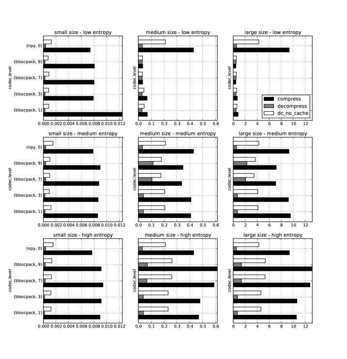
Figure 1: Compare Bloscpack and NPY on the SSD storage type.

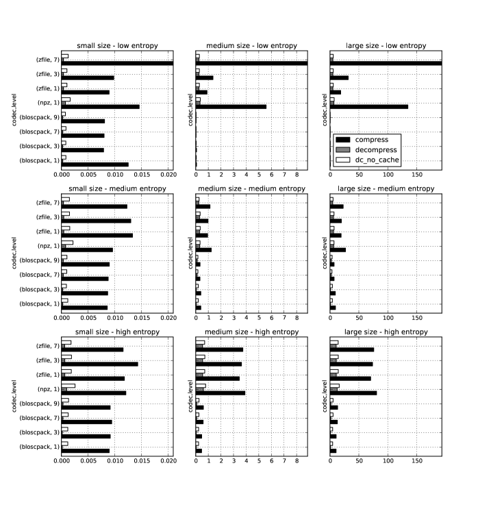
Figure 2: Compare Bloscpack, NPZ and ZFile on the SSD storage type.

Figure 3: Compare Bloscpack and NPY on the SD storage type.

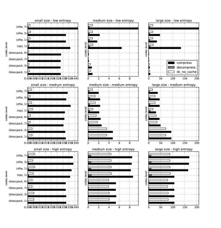
Figure 4: Compare Bloscpack, NPZ and ZFile on the SD storage type.

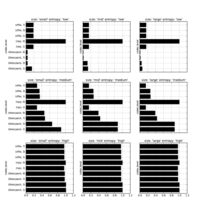
Figure 5: Compression ratios for all examined formats

In Fig. 1 we can see how Bloscpack compares to NPY on the SSD storage type. The first thing to note, is that for small datasets (first column of subplots), Bloscpack does not lag behind much compared to NPY for compression and is actually slightly faster for decompression. However the absolute differences here are in the millisecond range, so one might perhaps argue that Bloscpack and NPY are on par for small datasets. As soon as we move to the medium size datasets first gains can be seen. Especially for the low entropy case where Bloscpack beats NPY for both compression and decompression w/o file system cache. For the medium entropy case, Bloscpack is slightly faster for a few settings, at least for the compression and decompression cases. Surprisingly, for the decompression with a hot file system cache, Bloscpack is actually 2 times slower under the compression levels 7 and 9. One possibility for this might be that, even though the file contents are in memory, reading from the file necessitates an initial memory-to-memory copy, before the data can actually be decompressed. For the high entropy case, Bloscpack is mostly slightly slower than NPY. For the large dataset the results are simply a scaled version of the medium dataset size results and yield no additional insights.

Fig. 2 shows the comparison between Bloscpack, NPZ and ZFile on the SSD storage type. In this comparison, the speed of the Blosc compressor really shines. For every combination of dataset size and entropy the is a compression level for Bloscpack that can compress faster than any of the competitors. In the extreme case of the large size and the low entropy, Bloscpack is over 300 times faster during compression than NPZ (302 seconds for NPZ vs. 0.446 seconds for Bloscpack). Even for the high entropy case, where very very little compression is possible due to the statistics of the dataset, Bloscpack is significantly faster during compression. This is presumably because Blosc will try to compress a buffer, finish very quickly because there is no work to be done and then it simply copies the input verbatim.

One very surprising result here is that both NPZ and ZFile with level 7 take extraordinary amounts of time to compress the low entropy dataset. In fact they take the longest on the low entropy dataset compared to the medium and high entropies. Potentially this is related to the high Lempel-Ziv complexity of that dataset, as mentioned before. Recall that both NPZ and ZFile use the DEFLATE algorithm which belongs to the class of LZ77 dictionary encoders, so it may suffer since it no shuffle filter as in the case of Blosc is employed.

Figures 3. and 4. show the same results as figures 1. and 2. respectively but but for the SD storage class. Since the SD card is much slower than the SSD card the task is strongly IO bound and therefore benefits of compression can be reaped earlier. For example, Bloscpack level 7 is twice as fast as NPY during compression on the medium size medium entropy dataset. For the low entropy dataset at medium and large sizes, Bloscpack is about an order of magnitude faster. For the high entropy dataset Bloscpack is on par with NPY because the overhead of trying to compress but not succeeding is negligible due to the IO boundedness resulting from the speed of the SD card. When comparing Bloscpack to NPZ and ZFile on the SD card, the IO boundedness means that any algorithm that can achieve a high compression ratio in a reasonable amount of time will perform better. For example for medium size and medium entropy, NPZ is actually 1.6 times faster than Bloscpack during compression. As in the SSD case, we observe that NPZ and ZFile perform very slowly on low entropy data.

Lastly in Figure 5. we can see the compression ratios for each codec, size and entropy. This is mostly just a sanity check. NPY is always at 1, since it is a plain serialization format. Bloscpack gives better compression ratios for low entropy data. NPZ and ZFile give better compression ratios for the medium entropy data. And all serializers give a ratio close to zero for the high entropy dataset.

12 Conclusion

This article introduced the Bloscpack file-format and python reference implementation. The features of the file format were presented and compared to other serialization formats in the context of Numpy ndarrays. Benchmarking results are presented that show how Bloscpack can yield performance improvements for serializing Numpy arrays when compared to existing solutions under a variety of different circumstances.

13 Future Work

As for the results obtained so far, some open questions remain unsolved. First of all, it is not clear why Bloscpack at level 7 and 9 gives comparatively bad results when decompressing with a hot file system cache. Also the bad performance of ZFile and NPY on the so-called low entropy dataset must be investigated and perhaps an alternative can be found that is not biased towards Bloscpack. Additionally, some mathematical insights into the complexity reduction properties of Blosc’s shuffle filter would be most valuable.

Lastly, more comprehensive benchmarks need to be run. This means, first finding non-artificial benchmark datasets and establishing a corpus to run Bloscpack and the other solutions on. Furthermore, It would be nice to run benchmarks on other architectures for machines with more than 2 physical cores, non-uniform memory access and an NFS file-system as commonly found in compute clusters.

14 Gratitude

The author would like to thank the following people for advice, helpful comments and discussions: Pauli Virtanen, Gaël Varoquaux, Robert Kern and Philippe Gervais. Also, the author would like to specially thank Stéfan van der Walt and Francecs Alted for reviewing drafts of this paper.

References

- [Alted2009] Francesc Alted. The Data Access Problem EuroScipy 2009 Keynote Presentation http://www.blosc.org/docs/StarvingCPUs.pdf
- [Alted2010] Francesc Alted. Why modern CPUs are starving and what can be done about it, Computing in Science & Engineering, Vol. 12, No. 2. (March 2010), pp. 68-71 http://www.blosc.org/docs/StarvingCPUs-CISE-2010.pdf
- [DEFLATE] Peter. Deutsch DEFLATE Compressed Data Format Specification version 1.3 RFC1951 1996 http://tools.ietf.org/html/rfc1951
- [Haenel2013] Valentin Haenel. Introducing Bloscpack EuroScipy 2013 Presentation https://github.com/esc/euroscipy2013-talk-bloscpack
- [Jacob2009] Bruce Jacob. The Memory System: You Can’t Avoid It, You Can’t Ignore It, You Can’t Fake It Synthesis Lectures on Computer Architecture 2009, 77 pages,
- [VanDerWalt2011] Stefan Van Der Walt, S. Chris Colbert, Gaël Varoquaux The NumPy array: a structure for efficient numerical computation Computing in Science and Engineering 13, 2 (2011) 22-30
- [LZ77] Ziv, Jacob; Lempel, Abraham (May 1977). A Universal Algorithm for Sequential Data Compression. IEEE Transactions on Information Theory 23 (3): 337–343.
- [NPY] Robert Kern. The NPY format https://github.com/numpy/numpy/blob/master/doc/neps/npy-format.txt
- [Joblib] Joblib http://pythonhosted.org/joblib/
- [zlib] Zlib http://www.zlib.net/
- [gzip] Gzip http://www.gzip.org/
- [rsync] Rsync http://rsync.samba.org/
- [Blaze] Blaze http://blaze.pydata.org/
- [CArray] CArray http://carray.pytables.org/docs/manual/
- [Numpy] Numpy http://www.numpy.org/
- [FastLZ] FastLZ http://fastlz.org/
- [Snappy] Snappy http://code.google.com/p/snappy/
- [LZ4] LZ4 http://code.google.com/p/lz4/
- [Blosc] Blosc http://blosc.org
- [Bloscpack] Bloscpack https://github.com/Blosc/bloscpack
- [CPU] Intel® Core™ i7-3667U Processor