Unitarity, Crossing Symmetry and Duality of the S-matrix in Large N Chern-Simons Theories with Fundamental Matter

Abstract:

We present explicit computations and conjectures for $2\to 2$ scattering matrices in large $N$ $U(N)$ Chern-Simons theories coupled to fundamental bosonic or fermionic matter to all orders in the ’t Hooft coupling expansion. The bosonic and fermionic S-matrices map to each other under the recently conjectured Bose-Fermi duality after a level-rank transposition. The S-matrices presented in this paper may be regarded as relativistic generalization of Aharonov-Bohm scattering. They have unusual structural features: they include a non- analytic piece localized on forward scattering, and obey modified crossing symmetry rules. We conjecture that these unusual features are properties of S-matrices in all Chern-Simons matter theories. The S-matrix in one of the exchange channels in our paper has an anyonic character; the parameter map of the conjectured Bose-Fermi duality may be derived by equating the anyonic phase in the bosonic and fermionic theories.

1 Introduction

It has recently been conjectured that $U(N)$ Chern-Simons theories coupled to a multiplet of fundamental Wilson-Fisher bosons at level $k$ are dual to $U(|k|-N)$ Chern-Simons theories coupled to fundamental fermions at level $-k$. The evidence for this conjecture is threefold. First the spectrum of ‘single trace’ operators and the three point functions of these operators have also been computed exactly in the ’t Hooft limit, and have been found to match[1, 2, 3, 4, 5, 6]. Second the thermal partition functions of these theories have also been computed in the ’t Hooft large $N$ limit and have been shown to match [2, 1, 7, 8, 9, 10, 5]. Finally the duality described above has been demonstrated to follow from an extreme deformation of the known Giveon-Kutasov type duality [11, 12] between supersymmetric theories [13].

Assuming the duality described above does indeed hold, it is interesting to better understand the map that transforms bosons into fermions. Morally, we would like an explicit construction of the fundamental fermionic field $\psi_{a}(x)$ as a function of the fundamental bosonic fields ; such a formula cannot, however, be given precise meaning in the current context as $\psi_{a}(x)$ is not gauge invariant and its offshell correlators are ill-defined.

The on shell limit of correlators of the elementary bosonic and fermionic fields, however, are physical as they compute the S-matrix for the scattering of bosonic or fermionic quanta. As Chern-Simons theory has no propagating gluonic states, the S-matrix is free of soft gluon infrared divergences when the fundamental fields (bosons and fermions) are taken to be massive. An identity relating well-defined bosonic and fermionic S-matrices appears to be the closest we can come to a precise bosonization map. Motivated by this observation, in this paper we present a detailed study of $2\rightarrow 2$ S-matrices in Chern-Simons theories with fundamental bosonic and fermionic fields.

Even independent of the Bose-Fermi duality, it is interesting that it is possible to determine exact results for the S-matrix of these theories as a function of the ’t Hooft coupling constant $\lambda=\frac{N}{k}$. Exact results for scattering amplitudes as a function of a gauge coupling constant are rare, and should be studied when available for qualitative lessons. As we will see below, the explicit formulae for S-matrices presented in this paper turn out to possess several unfamiliar and unusual structural features. Some of these unusual features appear to have a simple physical interpretation; we anticipate that they are general properties of S-matrices in all matter Chern-Simons theories.

As we have mentioned above, it is possible to determine (or conjecture) explicit results for the $2\rightarrow 2$ scattering amplitudes for large $N$ fundamental matter Chern-Simons theories. In this paper we present explicit formulae for all these scattering amplitudes. In the rest of this introduction we will describe the most important qualitative features of our results. We first briefly review some kinematics in order to set terminology.

Consider the $2\rightarrow 2$ scattering of particles in representations $R_{1}$ and $R_{2}$ of $U(N)$. Let the tensor product of these two representations decompose as

$$R_{1}\times R_{2}=\sum_{m}R_{m}.$$ (1)

It follows from $U(N)$ invariance that the S-matrix for the process takes the schematic form

$$S=\sum_{m}P_{m}S_{m},$$ (2)

where $P_{m}$ is the projector onto the $m^{th}$ representation, and $S_{m}$ is the scattering matrix in the ‘$m^{th}$’ channel.

In this paper we study the $2\rightarrow 2$ scattering matrices of the elementary quanta of theories with only fundamental matter. In this situation $R_{1}$ and $R_{2}$, are either both fundamentals, or one fundamental and one antifundamental.  In the case of fundamental - fundamental scattering, $R_{m}$ is either the ‘symmetric’ representation with two boxes in the first row (and no boxes in any other row) of the Young Tableaux, or the ‘antisymmetric’ representation with two boxes in the first column and no boxes in any other column. In the case of fundamental - antifundamental scattering, $R_{m}$ is either the singlet or the adjoint representation. In this paper we will present computations or conjectures for the all orders S-matrices in all the four channels mentioned above (symmetric, antisymmetric, singlet and adjoint) in both the bosonic and the fermionic theories.

The scattering matrices of interest to us in this paper are already well known in the non-relativistic limit (i.e. in the limit in which the masses of the scattering particles and the center of mass energy are both taken to infinity at fixed momentum transfer) as we now very briefly review. The Chern-Simons equation of motion ensures that each particle traps magnetic flux. The Aharonov-Bohm effect then ensures that the particle $R_{1}$ picks up the phase $2\pi\nu_{m}$ as it circles around the particle $R_{2}$, where

$$2\pi\nu_{m}=\frac{4\pi T_{1}^{a}T_{2}^{a}}{k}=2\pi\frac{C_{2}(R_{m})-C_{2}(R_{1})-C_{2}(R_{2})}{k},$$ (3)

(where $T_{1/2}^{a}$ are the representation matrices for the group generators in representations $R_{1}$ and $R_{2}$ and $C_{2}(A)$ is the quadratic Casimir in representation $A$). It follows as a consequence [14] that the non-relativistic scattering amplitude in the $R_{m}$ exchange channel is given by the Aharonov-Bohm scattering amplitude of a $U(1)$ particle of unit charge of a point like magnetic flux of strength $2\pi\nu_{m}$.

It is easily verified that $\nu_{m}={\cal O}(\frac{1}{N})$ or smaller in the symmetric, antisymmetric or adjoint channels. In the singlet channel, however, it turns out that to leading order in the large $N$ limit $\nu_{m}=\frac{N}{k}=\lambda$. It follows that the rotation by $\pi$ which interchanges the two scattering particles is accompanied by a phase $e^{-i\pi\lambda_{B}}$ in the bosonic theory and $(-1)e^{-i\pi\lambda_{F}}=e^{-i\pi(-{\rm sgn}(\lambda_{F})+\lambda_{F})}$ in the fermionic theory. Note that these phases are identical when

$$\lambda_{B}=\lambda_{F}-{\rm sgn}(\lambda_{F}).$$ (4)

However (4) is precisely the map between $\lambda_{B}$ and $\lambda_{F}$ [5] induced by the level-rank duality transformation described at the beginning of this introduction. In the singlet channel, in other words the bosons and conjecturally dual fermions are both effectively anyonic, with the same anyonic phase. This observation provides a partial physical explanation for the duality map (4).

We note in passing that the anyonic phase $\pi\lambda_{B}$ is precisely twice the phase of the bulk interaction term in the conjectured Vasiliev duals to these theories [1, 15]. Indeed the first speculation of the bosonization duality for matter Chern-Simons theories [1] was motivated by argument very similar to that presented in the previous paragraph but in the context of Vasiliev theories (deformations of the bosonic and fermionic theory that lead to the same interaction phase ought to be the same theory). It would certainly be very interesting to find a logical link between the phase of interactions in Vasiliev theory and the anyonic phase of the previous paragraph, but we will not peruse this thread in this paper.

Moving away from the non-relativistic limit, in this paper we have (following the lead of [5]) summed all planar graphs to determine the exact relativistic S-matrix for both the bosonic as well as the fermionic theories in the symmetric, antisymmetric and adjoint channels. Even though our completely explicit solutions are quite simple, they possess a rich analytic structure (see section 3 for a detailed listing of results). It is a simple matter to compare the explicit results for the S-matrices in the bosonic and fermionic theories that are conjecturally dual to each other. We find that the bosonic and fermionic S-matrices agree perfectly in the adjoint channel. On the other hand the bosonic S-matrix in the symmetric/antisymmetric channels matches the fermionic S-matrix in the antisymmetric/symmetric channels. Our results are all consistent with the following rule: the bosonic S-matrix in the exchange channel $R_{m}$ is identical with the fermionic S-matrix in the exchange channel $R_{m}^{T}$, where $R_{m}^{T}$ is the dual representation under level-rank duality.

The match of S-matrices upto transposition appears to make perfect sense from several points of view. Let us focus attention on the particle - particle scattering and consider a multi-particle asymptotic state. As the Aharonov-Bohm phases $\nu_{m}$ vanish in the large $N$ limit considered in this paper, the multi-particle state in question is effectively a collection of non interacting bosonic particles, and so must obey Bose statistics. As an example, consider a multi-particle state that is completely antisymmetric under the interchange of its momenta. In order to meet the requirement of Bose statistics, this state must also be completely antisymmetric under the interchange of color indices. The corresponding dual asymptotic state in the fermionic theory is also completely antisymmetric under the interchange of momenta. In order to meet the requirement of fermionic statistics, this state must thus be completely symmetric under the interchange of color indices. In other words the map between bosonic and fermionic asymptotic states must involve a transposition of color representations; this transposition is part of the duality map between asymptotic states of the two theories, and is a reflection of the bose -fermi nature of the duality. See section 8 for further discussion of the map between the multi-particle states of this theory induced by duality.

The transposition of exchange representations above might also have been anticipated from another point of view. In the pure gauge sector (i.e. upon decoupling the fundamental bosonic and fermionic fields by making them very massive), the conjectured duality between the bosonic and fermionic theories reduces to the level-rank duality between two distinct pure Chern-Simons theories. It is well known that, under level-rank duality, a Wilson line in representation $R$ maps to a Wilson line in the representation $R^{T}$. As a Wilson line in representation $R$ represents the trajectory of a particle in representation $R$, it seems very natural that the exchange channels in a dynamical scattering process also map to each other only after a transposition.

Before proceeding we pause to address an issue of possible confusion. We have asserted above that scalar and spinor S-matrices map to each other under duality. The reader whose intuition is built from the study of four dimensional scattering processes may find this confusing. Scalar and spinor S-matrices cannot be equated in four or higher dimensions as they are functions of different variables. Scalar S-matrices are labelled by the momenta of the participating particles. On the other hand spinor S-matrices are labelled by both the momentum and the ‘polarization spinor’ of the participating particles. In precisely three dimensions, however, the Dirac equation uniquely determines the polarization spinor of particles and antiparticles as a function of of their momenta . It follows that three dimensional spinorial and scalar S-matrices are both functions only of the momenta of the scattering particles, so these S-matrices can be sensibly identified.

For a technical reason we explain below we are unable to directly compute the S-matrix in the singlet exchange channel by summing graphs; given this technical limitation we are constrained to simply conjecture a result for this S-matrix. The reader familiar with the usual lore on scattering matrices may think this is an easy task. According to traditional wisdom, the S-matrices in a relativistic quantum field theory enjoy crossing symmetry. Particle-antiparticle scattering in both channels should be determined from the results of particle-particle scattering; given the scattering amplitudes in the symmetric and antisymmetric exchange channels, we should be able to obtain the results of scattering in the singlet and adjoint exchange channels by analytic continuation. This principle yields a conjecture for the S-matrix in the singlet channel which, however, fails every consistency check: it has the wrong non relativistic limit and does not obey the constraints of unitarity. For this reason we propose that the usual rules of crossing symmetry are modified in the study of S-matrices in matter Chern Simons theories.

A hint that crossing symmetry might be complicated in these theories is present already in the non-relativistic limit as the Aharonov-Bohm scattering amplitude has an unusual $\delta$ function contribution localized about forward scattering [16]. This contribution to the S-matrix has a simple physical origin: a wave packet of one particle that passes through another is diluted by the factor $\cos(\pi\nu_{m})$ compared to the usual expectations because of destructive interference from Aharonov-Bohm phases; as a consequence the S-matrix includes a term proportional to $(\cos(\pi\nu_{m})-1)I$ ($I$ is the identity S matrix; see subsection 2.3 for more details). The non-analyticity of this term makes it difficult to imagine it can be obtained from a procedure involving analytic continuation.

In addition to the singular $\delta$ function piece, the scattering amplitude has an analytic part. In this paper (and in the large $N$ limit studied here) we conjecture that this analytic piece is given by the naive analytic continuation from the particle-particle sector, multiplied by the factor

$$f(\lambda)=\frac{\sin(\pi\lambda)}{\pi\lambda}.$$

This conjecture passes several consistency checks; it yields a result consistent with the expectations of unitarity, and has the right non-relativistic limit, and yields $S$-channel S-matrices that transform into each other under Bose-Fermi duality.

The factor $f(\lambda)$ is familiar in the study of pure Chern-Simons theory; $N$ times this factor is the expectation value of a circular Wilson loop on $S^{3}$ in the large $N$ limit. In section 7.4 below we present a tentative explanation for why one should have expected S-matrices in matter Chern-Simons theories to obey the modified analyticity relation with precisely the factor $f(\lambda)$. Our tentative explanation has its roots in the fact that the fully gauge invariant object that obeys crossing symmetry is the ‘S-matrix’ computed in this paper dressed with external Wilson lines linking the scattering particles. The presence of the Wilson lines leads to an additional contribution (in addition to those considered in this paper) that we argue to be channel dependent; in fact we argue that the ratio of the additional contributions in the two channels is precisely the given by the factor above, explaining why the ‘bare’ S-matrix computed in this paper has ‘renormalized’ crossing symmetry properties. If our tentative explanation of this feature is along the right tracks, then it should be possible to find a refined argument that predicts the analytic structure and crossing properties of the S-matrix at finite values of $N$ and $k$. We leave this exciting task for the future.

We note also that the factor $f(\lambda)$ appears also in the normalization of two point functions of, for instance, two stress tensors (see [5]). The appearance of this factor in the two point functions of gauge invariant operators seems tightly tied to the appearance of the same factor in scattering in the singlet channel, as the diagrams that contribute to these processes are very similar. It would be interesting to understand this relationship better.

This paper is organized as follows. In section 2 below we describe the theories we study in this paper, review the conjectured level-rank dualities between the bosonic and fermionic theories, set up the notation and conventions for the scattering process we study, review the constraints of unitarity on scattering and review the known non-relativistic limits of the scattering matrices. In section 3 below we briefly summarize the method we use to compute S-matrices, and provide a detailed listing of the principal results and conjectures of our paper. We then turn to a systematic presentation of our results. In section 4 we compute the S-matrices of the bosonic theories by solving the relevant Schwinger-Dyson equations. In section 5 we verify the results of section 4 at one loop by a direct diagrammatic evaluation of the S-matrix in the covariant Landau gauge. In section 6 we compute the S-matrix of the fermionic theories by solving a Schwinger-Dyson equation and verify the equivalence of our bosonic and fermionic results under duality. In section 7 we present our conjecture for the $S$-channel scattering amplitudes (in the bosonic and fermionic systems) of our theory, and provide a heuristic explanation for the unusual transformation properties under crossing symmetry obeyed by our conjecture. In section 8 we end with a discussion of our results and of promising future directions of research. Several appendices contain technical details of the computations presented in this paper.

2 Statement of the problem and review of background material

This section is organized as follows. In subsection 2.1 we describe the theories we study. In subsection 2.2 we review the conjectured duality between the bosonic and fermionic theories. In subsection 2.3 we review relevant aspects of the kinematics of $2\rightarrow 2$ scattering in 3 dimensions, with particular emphasis on the structure of the ‘identity’ scattering amplitude, which will turn out to be renormalized in matter Chern-Simons theories. In subsection 2.4 describe the precise scattering processes we study in this paper. In subsection 2.6 we review the known non-relativistic limits of these scattering amplitudes. In subsection 2.7 we describe the constraints on these amplitudes from the requirement of unitarity.

2.1 Theories

As we have explained above, in this paper we study two classes of large $N$ Chern-Simons theories coupled to matter fields in the fundamental representation. The first family of theories we study involves a single complex bosonic field, in the fundamental representation of $U(N)$, minimally coupled to a Chern-Simons coupled gauge field. In the rest of this paper we refer to this class of theories as ‘bosonic theories’. The second family of theories we study involves a single complex fermionic field in the fundamental representation of $U(N)$, minimally coupled to a Chern-Simons coupled gauge field. In the rest of this paper we refer to this class of theories as ‘fermionic theories’.

The bosonic system we study is described by the Euclidean Lagrangian

$$S =\int d^{3}x\biggl{[}i\varepsilon^{\mu\nu\rho}\frac{k_{B}}{4\pi}\mathrm{Tr}(A_{\mu}\partial_{\nu}A_{\rho}-\frac{2i}{3}A_{\mu}A_{\nu}A_{\rho})+D_{\mu}\bar{\phi}D^{\mu}\phi+m_{B}^{2}\bar{\phi}\phi+\frac{1}{2N_{B}}b_{4}(\bar{\phi}\phi)^{2}\biggl{]}$$ (5)

with $\lambda_{B}=\frac{N_{B}}{k_{B}}$. Throughout this paper we employ the dimensional regularization scheme and light cone gauge employed in the original study of [1]. The theory (5) has been studied intensively in the recent literatures [5, 2, 8, 6, 7, 13, 9, 10, 17, 4]. It has in particular been demonstrated that in the regulation scheme and gauge employed in this paper, the bosonic propagator is given, at all orders in $\lambda_{B}$, by the extremely simple form

$$\begin{split}\langle{\phi_{j}(p)\bar{\phi}}^{i}(-q)\rangle&=\frac{(2\pi)^{3}\delta^{i}_{j}\delta^{3}(-p+q)}{p^{2}+c_{B}^{2}}\\ \end{split}$$ (6)

where the pole mass, $c_{B}$ is a function of $m_{B},b_{4}$ and $\lambda_{B}$, given by

$$c_{B}^{2}=\frac{\lambda_{B}^{2}}{4}c_{B}^{2}-\frac{b_{4}}{4\pi}|c_{B}|+m_{B}^{2}.$$ (7)

(see e.g. Eqn $1.5$ of [13] setting $x_{4}=0$ setting temperature $T$ to zero). In all the Feynman diagrams presented in this paper, we adopt the following convention. The propagator (6) is denoted by a line with an arrow from ${\bar{\phi}}$ to $\phi$, with moment $p$ in the direction of the arrow (see Fig. 1).

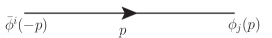
Figure 1: Propagator of bosonic particles.

The fermionic system we study is described by the Lagrangian

$$S =\int d^{3}x\biggl{[}i\varepsilon^{\mu\nu\rho}\frac{k_{F}}{4\pi}\mathrm{Tr}(A_{\mu}\partial_{\nu}A_{\rho}-\frac{2i}{3}A_{\mu}A_{\nu}A_{\rho})+\bar{\psi}\gamma^{\mu}D_{\mu}\psi+m_{F}\bar{\psi}\psi\biggl{]}$$ (8)

with $\lambda_{F}=\frac{N_{F}}{k_{F}}$. This theory has also been studied intensively in the recent literatures [8, 6, 7, 13, 9, 10, 17, 1, 4]. In particular it has been demonstrated that the fermionic propagator is given (in the light cone gauge and dimensional regulation scheme of this paper), to all orders in $\lambda_{F}$, by [1, 8, 6, 13]

$$\begin{split}\left\langle\psi_{j}(p)\bar{\psi}^{i}(-q)\right\rangle&=\frac{\delta^{i}_{j}(2\pi)^{3}\delta^{3}(-p+q)}{i\gamma^{\mu}p_{\mu}+\Sigma_{F}(p)},\end{split}$$ (9)

where

$${\Sigma_{F}}(p)= i\gamma^{\mu}\Sigma_{\mu}(p)+\Sigma_{I}(p)I,$$

$$\Sigma_{I}(p)= m_{F}+\lambda_{F}\sqrt{c_{F}^{2}+p_{s}^{2}},$$

$$\Sigma_{\mu}(p)= \delta_{+\mu}\frac{p_{+}}{p_{s}^{2}}\left(c_{F}^{2}-\Sigma_{I}^{2}(p)\right),$$

$$c_{F}^{2}= \left(\frac{{m_{F}}}{{\rm sgn}(m_{F})-\lambda_{F}}\right)^{2}.$$ (10)

Here $\gamma^{\mu}$ compose the Euclidean Clifford algebra,

$$\{\gamma^{\mu},\gamma^{\nu}\}=2\delta^{\mu\nu},\quad[\gamma^{\mu},\gamma^{\nu}]=2i\epsilon^{\mu\nu\rho}\gamma_{\rho}.$$

The fermionic propagator presented above has a pole at $p^{2}=c_{F}^{2}$; so the quantity $c_{F}$ is the pole mass - or true mass - of the fermionic quanta . In all the Feynman diagrams presented in this paper, we adopt the following convention. The propagator (9) is denoted by a line with an arrow from $\bar{\psi}$ to $\psi$, with momentum $p$ in the direction of the arrow (see Fig. 2).

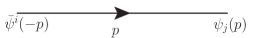
Figure 2: Propagator of fermionic particles.

2.2 Conjectured Bose-Fermi duality

The bosonic theory (5) may be rewritten as

$$\begin{split}S=&\int d^{3}x\biggl{[}i\varepsilon^{\mu\nu\rho}\frac{k_{B}}{4\pi}\mathrm{Tr}(A_{\mu}\partial_{\nu}A_{\rho}-\frac{2i}{3}A_{\mu}A_{\nu}A_{\rho})+D_{\mu}\bar{\phi}D^{\mu}\phi+m_{B}^{2}\bar{\phi}\phi+\frac{1}{2N_{B}}b_{4}(\bar{\phi}\phi)^{2}\\ &-\frac{N_{B}}{2b_{4}}\left(\sigma-\frac{b_{4}}{N_{B}}{\bar{\phi}\phi}-m_{B}^{2}\right)^{2}\biggl{]}.\end{split}$$ (11)

We have introduced a new field $\sigma$ in (11); upon integrating $\sigma$ out (11) trivially reduces to (5). Expanding out the last bracket in (11) and ignoring the constant term, we find that (11) may be rewritten as

$$S=\int d^{3}x\biggl{[}i\varepsilon^{\mu\nu\rho}\frac{k_{B}}{4\pi}\mathrm{Tr}(A_{\mu}\partial_{\nu}A_{\rho}-\frac{2i}{3}A_{\mu}A_{\nu}A_{\rho})+D_{\mu}\bar{\phi}D^{\mu}\phi+\sigma{\bar{\phi}}\phi+N_{B}\frac{m_{B}^{2}}{b_{4}}\sigma-N_{B}\frac{\sigma^{2}}{2b_{4}}\biggl{]}.$$ (12)

The so called Wilson-Fisher limit of the bosonic theory is obtained by taking the limit

$$b_{4}\to\infty,~{}~{}~{}m_{B}\to\infty,~{}~{}~{}\frac{4\pi m_{B}^{2}}{b_{4}}=m_{B}^{{\rm cri}}={\rm fixed}.$$ (13)

In this limit the last term in (12) may be omitted; moreover it follows from (7) that in this limit

$$|c_{B}|=m_{B}^{{\rm cri}}.$$

Note, of course, that this equation has no solution for negative $m_{B}^{{\rm cri}}$. As was explained in [5, 13] this is plausibly a reflection of the fact that (7) is the saddle point equation for an uncondensed solution, whereas the scalar in the theory wants to condense when $m_{B}^{{\rm cri}}<0$. The determination of the condensed saddle point is a fascinating but unsolved problem, and in this paper we restrict our attention to the case $m_{B}^{{\rm cri}}>0$.

As we have mentioned in the introduction, it has been has been conjectured that the scalar theory in the Wilson-Fisher limit described above is dual to the theory (8), once we identify parameters according to

$$\begin{split}k_{F}&=-k_{B},\\ N_{F}&=|k_{B}|-N_{B},\\ \lambda_{B}&=\lambda_{F}-{\rm sgn}(\lambda_{F}),\\ m_{F}&=-m_{B}^{{\rm cri}}\lambda_{B}.\\ \end{split}$$ (14)

As we have explained above, we will restrict our attention to bosonic theories with $m_{B}^{{\rm cri}}>0$. It follows from (14) that, for the purpose of studying the bose-fermi duality, we should restrict attention to fermionic theories that obey the inequality

$$\lambda_{F}m_{F}>0.$$ (15)

It is easily verified that (14) implies that

$$|c_{F}|=|c_{B}|.$$ (16)

In other words the bosonic and fermionic fields have equal pole masses under duality. This observation already makes it seem likely that the duality map should involve some sort of identification of elementary bosonic and fermionic quanta. The relationship between bosonic and fermionic S-matrices, proposed in this paper, helps to flesh this identification out.

2.3 Scattering kinematics

In this paper we study $2\rightarrow 2$ particle scattering; for this purpose we work in Minkowski space. Let the 3 momenta of the initial particles be denoted by $p_{1}$ and $p_{2}$ and let the momenta of the final particles be denoted by $-p_{3}$ and $-p_{4}$. Momentum conservation ensures $p_{1}+p_{2}+p_{3}+p_{4}=0$. We use the mostly positive sign convention, and define the Lorentz invariants $s,t,u$ in the usual manner

$$s=-(p_{1}+p_{2})^{2},~{}~{}t=-(p_{1}+p_{3})^{2},~{}~{}u=-(p_{1}+p_{4})^{2},~{}~{}s+t+u=4c_{B}^{2}$$ (17)

where $c_{B}$ is the pole mass of the scattering particles (the scattering particles have equal mass).

The $S$ matrix for the scattering processes is given by (see below for slight modifications to deal with bosonic or fermionic statistics)

$$\begin{split}{\bf S}(p_{1},p_{2},-p_{3},-p_{4})=&(2E_{{\vec{p}}_{1}})(2\pi)^{2}\delta^{2}({\vec{p}}_{1}+{\vec{p}}_{3})(2E_{{\vec{p}}_{2}})(2\pi)^{2}\delta^{2}({\vec{p}}_{2}+{\vec{p}}_{4})\\ &+i(2\pi)^{3}\delta^{3}(p_{1}+p_{2}+p_{3}+p_{4})T(s,t,u,E(p_{1},p_{2},p_{3})),\\ E_{{\vec{p}}}=&\sqrt{c_{B}^{2}+{\vec{p}}^{2}},\\ E(p_{1},p_{2},p_{3})=&\pm 1={\rm sgn}\left(\epsilon_{\mu\nu\rho}p_{1}^{\mu}p_{2}^{\nu}p_{3}^{\rho}\right),~{}~{}~{}\epsilon_{012}=-\epsilon^{012}=1\end{split}$$ (18)

The fact that $2\rightarrow 2$ scattering can depend on the $Z_{2}$ valued variable $E(p_{1},p_{2},p_{3})$ rather than just $s,t,u$ is a kinematical peculiarity of 3-dimenensions. Note that $E(p_{1},p_{2},p_{3})$ measures the ‘handedness’ of the triad of vectors $p_{1},p_{2},p_{3}$. The symbol ${\vec{p}}$ that appears in (18) denotes the spatial part of the 3-vector $p$. It might seem to be strange that ${\vec{p}}$ makes any appearance in the formula for a Lorentz covariant S-matrix. Note, however, that the various 3-vectors we deal with are always on-shell, so the knowledge of ${\vec{p}}$ is sufficient to permit the reconstruction of the full 3-vector $p$. Using the on-shell condition it is not difficult to verify that $(2E_{\vec{p}})(2\pi)^{2}\delta^{2}({\vec{p}}+{\vec{r}})$ is Lorentz invariant, even though this is not completely manifest.

The manifestly Lorentz invariant rule for the multiplication of two S-matrices is

$$\begin{split}&[{\bf S_{1}S_{2}}](p_{1},p_{2},-p_{3},-p_{4})\\ =&\int\frac{d^{3}r_{1}(2\pi)\theta(r_{1}^{0})\delta(r_{1}^{2}+c_{B}^{2})}{(2\pi)^{3}}\frac{d^{3}r_{2}(2\pi)\theta(r_{2}^{0})\delta(r_{2}^{2}+c_{B}^{2})}{(2\pi)^{3}}\\ &~{}~{}\times{\bf S_{1}}(p_{1},p_{2},-r_{1},-r_{2}){\bf S_{2}}(r_{1},r_{2},-p_{3},-p_{4})\\ =&\int\frac{d^{2}{\vec{r}}_{1}}{2E_{{\vec{r}}_{1}}(2\pi)^{2}}\frac{d^{2}{\vec{r}}_{2}}{2E_{{\vec{r}}_{2}}(2\pi)^{2}}{\bf S_{1}}(p_{1},p_{2},-r_{1},-r_{2}){\bf S_{2}}(r_{1},r_{2},-p_{3},-p_{4}).\\ \end{split}$$ (19)

The quantity

$$I(p_{1},p_{2},-p_{3},-p_{4})=(2E_{{\vec{p}}_{1}})(2\pi)^{2}\delta^{2}({\vec{p}}_{1}+{\vec{p}}_{3})(2E_{{\vec{p}}_{2}})(2\pi)^{2}\delta^{2}({\vec{p}}_{2}+{\vec{p}}_{4})$$ (20)

that appears in the first line of (18) is clearly the identity matrix for this multiplication rule.

The identity matrix may be rewritten in a manifestly Lorentz invariant form (see Appendix A )

$$I(p_{1},p_{2},-p_{3},-p_{4})=\lim_{\epsilon\to 0}4\pi\sqrt{s}\delta\left(\sqrt{\frac{4t}{t+u}}-\epsilon\right)(2\pi)^{3}\delta^{3}(p_{1}+p_{2}+p_{3}+p_{4}).$$ (21)

It is sometimes convenient to study $2\rightarrow 2$ scattering in the center of mass frame. In this frame the scattering momenta may be taken to be

$$\begin{split}&p_{1}=(\sqrt{k^{2}+c_{B}^{2}},k,0),~{}~{}~{}p_{2}=(\sqrt{k^{2}+c_{B}^{2}},-k,0)\\ &p_{3}=(-\sqrt{k^{2}+c_{B}^{2}},-k\cos(\theta),-k\sin(\theta)),~{}~{}~{}p_{4}=(-\sqrt{k^{2}+c_{B}^{2}},k\cos(\theta),k\sin(\theta)).\\ \end{split}$$ (22)

The kinematical invariants are given by

$$s=4(c_{B}^{2}+k^{2}),~{}~{}~{}t=-2k^{2}\left(1-\cos(\theta)\right),~{}~{}~{}u=-2k^{2}\left(1+\cos(\theta)\right),$$ (23)

and the S-matrix takes the form

$${\bf S}=(2\pi)^{3}\delta(p_{1}+p_{2}+p_{3}+p_{4})S(\sqrt{s},\theta),$$ (24)

where $\theta$ is the scattering angle - the angle between $-{\vec{p}}_{3}$ and ${\vec{p}}_{1}$. More precisely, let ${\vec{p}}_{1}$ point along the positive $x$ axis so that ${\vec{p}}_{2}$ points along the negative $x$ axis. $\theta\in(-\pi,\pi)$ is defined as the rotation in the clockwise direction (here clockwise is defined w.r.t. the orientation of the usual $x,y$ axis system) that is needed to rotate ${\vec{p}}_{1}$ into $-{\vec{p}}_{3}$. Note that parity transformations, that take $\theta$ to $-\theta$, are generically not symmetries of our theory. In the center of mass system $E(p_{1},p_{2},p_{3})$ defined in (18) is given by

$$E(p_{1},p_{2},p_{3})={\rm sgn}(\theta).$$ (25)

For later use we note the following center of mass reduction formulae

$$\begin{split}E(p_{1},p_{2},p_{3})\sqrt{\frac{su}{t}}&\rightarrow\sqrt{s}\cot\left(\frac{\theta}{2}\right),\\ E(p_{1},p_{2},p_{3})\sqrt{\frac{st}{u}}&\rightarrow\sqrt{s}\tan\left(\frac{\theta}{2}\right),\\ E(p_{1},p_{2},p_{3})\sqrt{\frac{tu}{s}}&\rightarrow\frac{2k^{2}}{\sqrt{s}}\sin(\theta).\\ \end{split}$$ (26)

The rule (19) induces the following multiplication rule for the functions $S(\sqrt{s},\theta)$:

$$[S_{1}S_{2}](\sqrt{s},\theta)=\int\frac{d\alpha}{8\pi\sqrt{s}}S_{1}(\sqrt{s},\alpha)S_{2}(\sqrt{s},\theta-\alpha),$$ (27)

The identity matrix for this multiplication rule is clearly given by

$$S_{I}(\sqrt{s},\theta)=8\pi\sqrt{s}\delta(\theta)=\lim_{\epsilon\to 0}4\pi\sqrt{s}\left[\delta(\theta+\epsilon)+\delta(\theta-\epsilon)\right],$$ (28)

in agreement with (21) recast in center of mass coordinates.

The Hermitian conjugate of an S-matrix functions for $S^{\dagger}$ are given by

$$\begin{split}&[{\bf S}^{\dagger}](p_{1},p_{2},-p_{3},-p_{4})={\bf S}^{*}(p_{3},p_{4},-p_{1},-p_{2}),\\ &[S^{\dagger}](\sqrt{s},\theta)=S^{*}(\sqrt{s},-\theta).\\ \end{split}$$ (29)

The S-matrix must be unitary, i.e. must obey the equation $S^{\dagger}S=1$. This implies

$$-i(T-T^{\dagger})=T^{\dagger}T.$$ (30)

Written out as an explicit equation for the $T$ functions this boils down to

$$\begin{split}&-i\left(T(p_{1},p_{2},-p_{3},-p_{4})-T^{\ast}(p_{3},p_{4},-p_{1},-p_{2})\right)\delta^{3}(p_{1}+p_{2}+p_{3}+p_{4})\\ &=\int\frac{d^{3}l}{(2\pi)^{3}}\frac{d^{3}r}{(2\pi)^{3}}\biggl{[}\theta(-l_{0})\theta(-r_{0})\delta^{3}(p_{1}+p_{2}+p_{3}+p_{4})\delta^{3}(p_{1}+p_{2}+l+r)\\ &~{}~{}~{}~{}~{}~{}~{}~{}~{}~{}~{}\times(2\pi)\delta(r^{2}+c_{B}^{2})(2\pi)\delta(l^{2}+c_{B}^{2})T^{*}(-p_{1},-p_{2},l,r)T(-p_{3},-p_{4},l,r)\biggr{]}+\ldots\end{split}$$ (31)

where the $\ldots$ denotes the contribution of intermediate states with more than two particles. We will return to this formula below

2.4 Channels of scattering

A theory of a fundamental field has two kinds of elementary quanta: those that transform in the fundamental of $U(N)$ and those that transform in the antifundamental of that gauge group. In this paper we refer to quanta in the fundamental of $U(N)$ as particles; we refer to quanta in the antifundamental of $U(N)$ as antiparticle. We use the symbol $P_{i}(p)$ to denote a particle with color index $i$ and three momentum $p$, while $A^{i}(p)$ denotes an antiparticle with color index $i$ and three momentum $p$. We employ this notation for both the bosonic and the fermionic theories described in the previous subsection.

In this paper we study $2\rightarrow 2$ scattering. There are essentially two distinct $2\rightarrow 2$ scattering process; particle-particle scattering and Particle-antiparticle scattering

2.4.1 Particle - antiparticle scattering

The tensor product of a fundamental and an antifundamental consists of the adjoint and the singlet representations. It follows that Particle-antiparticle scattering is characterized by two scattering functions. We adopt the following terminology: we refer to scattering in the singlet channel as scattering in the $S$-channel. Scattering in the adjoint channel is referred to as scattering in the $T$-channel.

It follows from $U(N)$ invariance that the S-matrix for the process

$$P_{i}(p_{1})+A^{j}(p_{2})\rightarrow P_{m}(-p_{3})+A^{n}(-p_{4})$$ (32)

is given by

$${\bf S}=\delta_{i}^{m}\delta^{j}_{n}I(p_{1},p_{2},-p_{3},-p_{4})+iT_{in}^{jm}(p_{1},p_{2},-p_{3},-p_{4})(2\pi)^{3}\delta^{3}(p_{1}+p_{2}+p_{3}+p_{4}).$$ (33)

(see the previous subsection for the definition of $I$). The S-matrix may be decomposed into adjoint and singlet scattering matrices

$${\bf S}=\left(\delta_{i}^{m}\delta^{j}_{n}-\frac{\delta_{i}^{j}\delta^{m}_{n}}{N}\right)S_{T}+\frac{\delta_{i}^{j}\delta^{m}_{n}}{N}S_{S}$$ (34)

where

$$\begin{split}&{\bf S}_{T}=I(p_{1},p_{2},-p_{3},-p_{4})+iT_{T}(p_{1},p_{2},-p_{3},-p_{4})(2\pi)^{3}\delta^{3}(p_{1}+p_{2}+p_{3}+p_{4})\\ &{\bf S}_{S}=I(p_{1},p_{2},-p_{3},-p_{4})+iT_{S}(p_{1},p_{2},-p_{3},-p_{4})(2\pi)^{3}\delta^{3}(p_{1}+p_{2}+p_{3}+p_{4})\end{split}$$ (35)

and

$$T_{in}^{jm}(p_{1},p_{2},-p_{3},-p_{4})=\left(\delta_{i}^{m}\delta^{j}_{n}-\frac{\delta_{i}^{j}\delta^{m}_{n}}{N}\right)T_{T}(p_{1},p_{2},-p_{3},-p_{4})+\frac{\delta_{i}^{j}\delta^{m}_{n}}{N}T_{S}(p_{1},p_{2},-p_{3},-p_{4})$$ (36)

2.4.2 Particle - particle scattering

The tensor product of two fundamentals consists of the representation with two boxes in the first row of the Young Tableaux, and another representation with two boxes in the first column of the Young Tableaux. We refer to these two representations as the symmetric $U$-channel and the antisymmetric $U$-channel respectively. It follows that particle- particle scattering is characterized by the scattering functions in these two channels.

More quantitatively, the S-matrix for the process

$$P_{i}(p_{1})+P_{j}(p_{2})\rightarrow P_{m}(-p_{3})+P_{n}(-p_{4})$$ (37)

takes the form

$$\begin{split}{\bf S}&=\pm\delta_{i}^{m}\delta_{j}^{n}I(p_{1},p_{2},p_{3},p_{4})+\delta_{i}^{n}\delta_{j}^{m}I(p_{1},p_{2},p_{4},p_{3})\\ &+iT_{ij}^{mn}(p_{1},p_{2},p_{3},p_{4})(2\pi)^{3}\delta^{3}(p_{1}+p_{2}+p_{3}+p_{4})\end{split}$$ (38)

where the $\pm$ in the first line is for bosons/fermions. The S-matrix may be decomposed into the symmetric and antisymmetric channels

$${\bf S}=\frac{\delta_{i}^{n}\delta_{j}^{m}+\delta_{i}^{m}\delta_{j}^{n}}{2}{\bf S}_{U_{s}}+\frac{\delta_{i}^{n}\delta_{j}^{m}-\delta_{i}^{m}\delta_{j}^{n}}{2}{\bf S}_{U_{a}}$$ (39)

where

$$\begin{split}{\bf S}_{U_{s}}&=\pm I(p_{1},p_{2},p_{3},p_{4})+I(p_{1},p_{2},p_{4},p_{3})\\ &+iT_{U_{s}}(p_{1},p_{2},p_{3},p_{4})(2\pi)^{3}\delta(p_{1}+p_{2}+p_{3}+p_{4})\\ {\bf S}_{U_{a}}&=-(\pm)I(p_{1},p_{2},p_{3},p_{4})+I(p_{1},p_{2},p_{4},p_{3})\\ &+iT_{U_{a}}(p_{1},p_{2},p_{3},p_{4})(2\pi)^{3}\delta(p_{1}+p_{2}+p_{3}+p_{4}).\\ \end{split}$$ (40)

We will sometimes need to work with the direct and exchange scattering amplitudes (${\bf S}_{U_{d}}$ and ${\bf S}_{U_{e}}$) by

$${\bf S}=\delta_{i}^{m}\delta_{j}^{n}{\bf S}_{U_{d}}+\delta_{i}^{n}\delta_{j}^{m}{\bf S}_{U_{e}}$$ (41)

where

$$\begin{split}{\bf S}_{U_{d}}&=\pm I(p_{1},p_{2},p_{3},p_{4})+iT_{U_{d}}(p_{1},p_{2},p_{3},p_{4})(2\pi)^{3}\delta(p_{1}+p_{2}+p_{3}+p_{4})\\ {\bf S}_{U_{e}}&=I(p_{1},p_{2},p_{4},p_{3})+iT_{U_{a}}(p_{1},p_{2},p_{3},p_{4})(2\pi)^{3}\delta(p_{1}+p_{2}+p_{3}+p_{4})\\ \end{split}$$ (42)

where

$$\begin{split}{\bf S}_{U_{s}}={\bf S}_{U_{d}}+{\bf S}_{U_{e}},~{}~{}~{}{\bf S}_{U_{a}}={\bf S}_{U_{e}}-{\bf S}_{U_{d}},~{}~{}~{}T_{U_{s}}=T_{U_{d}}+T_{U_{e}},~{}~{}~{}T_{U_{a}}=T_{U_{e}}-T_{U_{d}}.\end{split}$$ (43)

And

$$T_{ij}^{mn}(p_{1},p_{2},p_{3},p_{4})=\delta_{i}^{m}\delta_{j}^{n}T_{U_{d}}(p_{1},p_{2},p_{3},p_{4})+\delta_{i}^{n}\delta^{m}_{j}T_{U_{e}}(p_{1},p_{2},p_{3},p_{4}).$$ (44)

We refer to $S_{U_{d}}$ as the ‘direct S-matrix’ in the $U$-channel. $S_{U_{e}}$, on the other hand is the ‘exchange S-matrix in the $U$-channel.

In this paper we study scattering in both the bosonic as well as fermionic theories described in the previous subsection. We use the superscript $B/F$ to denote the corresponding functions in the bosonic/fermionic theories. For example $S_{T}^{B}$ is the $T$-channel scattering matrix for bosons, while $S^{F}_{S}$ denotes the $S$-channel scattering matrix for fermions.

2.5 Tree level scattering amplitudes in the bosonic and fermionic theories

The evaluation of full S-matrix of the bosonic and fermionic theories of subsection 2.1 is the main subject of this paper. The evaluation of the all loop amplitudes will require summing all planar diagrams in lightcone gauge, together with some educated guesswork. However the tree level scattering amplitudes in these theories are, of course, easily evaluaed in a covariante Landau gauge. In this section we simply present the results for these tree level scattering amplitudes, in all scattering channels, in both the bosonic and the fermionic theories. In every case we present the results for the full $S$ matrix (rather than the $T$ matrix) to emphasize the relative sign between the identity piece and the scattering terms. In the scalar theories we work for simplicity at $b_{4}=0$. Our results in the fermionic theory are presented upto a physically irrelevant overall phase. The results presented in this subsection are all derived in Appendix B.

At tree level we find

$$\begin{split}{\bf S}_{B,U_{d}}&=I(p_{1},p_{2},p_{3},p_{4})-\frac{4\pi}{k_{B}}\frac{\epsilon_{\mu\nu\rho}p_{1}^{\mu}p_{2}^{\nu}p_{3}^{\rho}}{(p_{2}+p_{3})^{2}}(2\pi)^{3}\delta(p_{1}+p_{2}+p_{3}+p_{4})\\ {\bf S}_{B,U_{e}}&=I(p_{1},p_{2},p_{4},p_{3})+\frac{4\pi}{k_{B}}\frac{\epsilon_{\mu\nu\rho}p_{1}^{\mu}p_{2}^{\nu}p_{3}^{\rho}}{(p_{2}+p_{4})^{2}}(2\pi)^{3}\delta(p_{1}+p_{2}+p_{3}+p_{4})\\ {\bf S}_{B,T}&=I(p_{1},p_{2},p_{3},p_{4})+\frac{4\pi}{k_{B}}\frac{\epsilon_{\mu\nu\rho}p_{1}^{\mu}p_{2}^{\nu}p_{3}^{\rho}}{(p_{4}+p_{3})^{2}}(2\pi)^{3}\delta(p_{1}+p_{2}+p_{3}+p_{4})\\ {\bf S}_{B,S}&=I(p_{1},p_{2},p_{3},p_{4})-4\pi\lambda_{B}\frac{\epsilon_{\mu\nu\rho}p_{1}^{\mu}p_{2}^{\nu}p_{3}^{\rho}}{(p_{2}+p_{4})^{2}}(2\pi)^{3}\delta(p_{1}+p_{2}+p_{3}+p_{4})\\ {\bf S}_{F,U_{d}}&=I(p_{1},p_{2},p_{3},p_{4})+\frac{4\pi}{k_{F}}\left(\frac{\epsilon_{\mu\nu\rho}p_{1}^{\mu}p_{2}^{\nu}p_{3}^{\rho}}{(p_{2}+p_{3})^{2}}-2im_{F}\right)(2\pi)^{3}\delta(p_{1}+p_{2}+p_{3}+p_{4})\\ {\bf S}_{F,U_{e}}&=I(p_{1},p_{2},p_{4},p_{3})-\frac{4\pi}{k_{F}}\left(\frac{\epsilon_{\mu\nu\rho}p_{1}^{\mu}p_{2}^{\nu}p_{3}^{\rho}}{(p_{2}+p_{4})^{2}}+2im_{F}\right)(2\pi)^{3}\delta(p_{1}+p_{2}+p_{3}+p_{4})\\ {\bf S}_{F,T}&=I(p_{1},p_{2},p_{3},p_{4})-\frac{4\pi}{k_{F}}\left(\frac{\epsilon_{\mu\nu\rho}p_{1}^{\mu}p_{2}^{\nu}p_{3}^{\rho}}{(p_{4}+p_{3})^{2}}+2im_{F}\right)(2\pi)^{3}\delta(p_{1}+p_{2}+p_{3}+p_{4})\\ {\bf S}_{F,S}&=-I(p_{1},p_{2},p_{3},p_{4})+4\pi\lambda_{F}\left(\frac{\epsilon_{\mu\nu\rho}p_{1}^{\mu}p_{2}^{\nu}p_{3}^{\rho}}{(p_{2}+p_{4})^{2}}-2im_{F}\right)(2\pi)^{3}\delta(p_{1}+p_{2}+p_{3}+p_{4}).\\ \end{split}$$ (45)

2.6 The non-relativistic limit and Aharonov-Bohm scattering

As we have explained above, in this paper we wish to compute the $2\rightarrow 2$ scattering matrix of fundamental matter coupled to Chern-Simons theory. The result of this computation is already well known in the non-relativistic limit, i.e. the limit in which

$$\frac{s-4c_{B}^{2}}{4c_{B}^{2}}\to 0.$$ (46)

In this limit the S-matrix is obtained from the scattering of two non-relativistic particles interacting with a Chern-Simons gauge field. The quantum description of this system may be obtained by first eliminating the non dynamical gauge field in a suitable gauge and then writing down the effective two particle Schrodinger equation see e.g. [14]). Moving to center of mass and relative coordinates further simplifies the problem to the study of the quantum mechanics of a single particle interacting with a point like flux tube located at the origin. The S-matrix may then be read off from the scattering solution of Aharonov-Bohm [18] with one interesting twist; the effective value of the flux depends on the scattering channel.

Let the scattering particles transform in the representations $R_{1}$ and $R_{2}$ of $U(N)$. As we have reviewed in the introduction, if

$$R_{1}\times R_{2}=\sum_{m}R_{m}$$ (47)

then

$$S=\sum_{m}S_{m}P_{m}$$

where $P_{m}$ is the projector onto the representation $R_{m}$. It turns out that the scattering matrix in the $m^{th}$ channel $S_{m}$ is simply the Aharonov-Bohm scattering amplitude of a unit charge $U(1)$ particle scattering off a thin flux tube with integrated flux $2\pi\nu_{m}$ where

$$\nu_{m}=\frac{C_{2}(R_{m})-C_{2}(R_{1})-C_{2}(R_{2})}{k}.$$ (48)

Let $F$ denote the fundamental representation, $A$ the antifundamental representation, $S$ the ‘symmetric’ representation (with two boxes in the first row of the Young Tableaux, and no boxes in any other row), $AS$ the antisymmetric representation (with two boxes in the first column of the Young Tableaux, and no boxes in any other column), $Adj$ the adjoint representation and $I$ the and the singlet. The Casimirs of these representations are

$$\begin{split}&C_{2}(F)=C_{2}(A)=\frac{N^{2}-1}{2N},~{}~{}~{}C_{2}(S)=\frac{N^{2}+N-2}{N},~{}~{}~{}C_{2}(AS)=\frac{N^{2}-N-2}{N}\\ &C_{2}(Adj)=N,~{}~{}~{}C_{2}(I)=0.\end{split}$$ (49)

In the symmetric and antisymmetric exchange channels respectively (for particle-particle scattering)

$$\nu_{S}=\frac{1}{k}-\frac{1}{Nk},~{}~{}~{}\nu_{AS}=-\frac{1}{k}-\frac{1}{Nk}.$$ (50)

In the singlet and adjoint exchange channels respectively (for particle - antiparticle scattering)

$$\nu_{I}=-\lambda_{B}+\frac{1}{Nk},~{}~{}~{}\nu_{AdJ}=\frac{1}{Nk}.$$ (51)

Note that in the large $N$ limit, $\nu_{I}$ is of order unity, $\nu_{S}$ and $\nu_{AS}$ are both of order ${\cal O}(1/N)$ and $\nu_{Adj}$ is of order ${\cal O}(1/N^{2})$.

In the rest of this subsection we specialize to scattering in the scalar theory. As we have reviewed in great detail in Appendix C, the quantum mechanics of a non-relativistic scalar scattering of a point like flux tube with integrated flux $2\pi\nu$ admits a ‘scattering’ solution (the Aharonov Bohm solution), whose large radius asymptotics is given by

$$\psi(r)=e^{ikx}+e^{-i\frac{\pi}{4}}h(\theta)e^{ikr}\sqrt{\frac{2\pi}{kr}}$$ (52)

where

$$h(\theta)=2\pi\left(\cos(\pi\nu)-1\right)\delta(\theta)+\sin(\pi\nu)\left({\rm Pv}\cot\left(\frac{\theta}{2}\right)-i{\rm sgn}(\nu)\right)$$ (53)

where $Pv$ denotes the principal value. In the non-relativistic limit and in the center of mass frame the scattering amplitude $T$ is proportional to $h(\theta)$; more precisely

$$T(s,\theta)=-4ih(\theta)\sqrt{s}.$$ (54)

Using (23) (54) and (53) together imply the covariant prediction

$$\begin{split}T_{m}^{NR}(p_{1},p_{2},p_{3},p_{4},\lambda_{B},b_{4})=&-4i\sqrt{s}\sin(\pi\nu_{m})\left(E(p_{1},p_{2},p_{3})\sqrt{\frac{t}{u}}-i{\rm sgn}(\nu_{m})\right)\\ &-i(\cos(\pi\nu_{m})-1)I(p_{1},p_{2},p_{3},p_{4})\end{split}$$ (55)

(see (20) (21), (28) for a definition of $I$) where $T_{m}^{NR}$ is the non-relativistic limit of scattering in the $m^{th}$ channel, $\nu_{m}$ is the corresponding value of $\nu$ as described above.

(55) applies when the scattering particles are distinguishable (as in the case of particle - antiparticle scattering in the situation of interest to our paper). When the scattering particles are identical - as in the case of particle - particle scattering in our paper, $R_{1}=R_{2}=R$ and we have to add the contribution of exchange scattering. (55) is modified to

$$\begin{split}T_{m}^{NR}(p_{1},p_{2},p_{3},p_{4},\lambda_{B},b_{4})=&-4i\sqrt{s}\sin(\pi\nu_{m})\left(E(p_{1},p_{2},p_{3})\sqrt{\frac{t}{u}}-i{\rm sgn}(\nu_{m})\right)\\ &-i(\cos(\pi\nu_{m})-1)I(p_{1},p_{2},p_{3},p_{4})\\ &+a\biggl{[}-4i\sqrt{s}\sin(\pi\nu_{m})\left(-E(p_{1},p_{2},p_{3})\sqrt{\frac{u}{t}}-i{\rm sgn}(\nu_{m})\right)\\ &~{}~{}~{}~{}~{}~{}~{}~{}-i(\cos(\pi\nu_{m})-1)I(p_{2},p_{1},p_{3},p_{4})\biggr{]}\end{split}$$ (56)

where the sign $a=1$ if the $R_{3}$ is symmetric in the $Rs$ while $a=-1$ if $R_{3}$ is antisymmetric product of 2 $R$s (in the case that the scattering particles are fermionic, $a$ has an additional overall -1). In writing (56) we have used the fact that $E(p_{2},p_{1},p_{3})=-E(p_{1},p_{2},p_{3})$.

2.6.1 Non-relativistic limit of $S$-channel scattering

In the $S$-channel $\nu_{m}=\lambda_{B}$ in the large $N$ limit so the $S$-channel S-matrix must reduce, in the limit (46), to

$$\begin{split}(T^{S}_{B})^{NR}(p_{1},p_{2},p_{3},p_{4},\lambda_{B},b_{4})=&4i\sqrt{s}\sin(\pi\lambda_{B})\left(E(p_{1},p_{2},p_{3})\sqrt{\frac{t}{u}}+i{\rm sgn}(\lambda_{B})\right)\\ &-i(\cos(\pi\lambda_{B})-1)I(p_{1},p_{2},p_{3},p_{4}).\end{split}$$ (57)

This prediction for the non-relativistic limit of the S-matrix in the $S$-channel has several striking features.

• $T_{S}^{B}$ is not an analytic function of kinematic variables. The term proportional to the $\delta$ function in that expression is singular, and is infact proportional to the identity scattering matrix (see subsection 2.3).

• $T_{S}^{B}$ is not an analytic function of $\lambda_{B}$ at $\lambda_{B}=0$ (because of the term proportional to ${\rm sgn}(\lambda_{B})$. )

• $T_{S}^{B}$ is universal, in the sense that it is independent of $b_{4}$ in this limit.

As we will see below, the last two features are artifacts of the non-relativistic limit. On the other hand we will now argue that the last the term in (53) $\propto\delta(\theta)$ is an exact feature of the S-matrix at all energy scales.

The term proportional to $\delta(\theta)$ in (53) was infact missed in the original analysis by Aharonov and Bohm. The presence of this term was discovered much later by Ruijsenaars [16] (see also the later papers [19, 14, 20, 21] for further elaboration) where it was also pointed out that this contact term is necessary to unitarize Aharonov-Bohm scattering (see the next subsection for a review of this fact). In the rest of this subsection we will present a simple physical interpretation for this part of the Aharonov-Bohm S-matrix.

As we have reviewed extensively in (2.3), the scattering matrix is postulated the form $S=I+iT$ where the factor $I$ accounts for the unscattered part of the wave packet. In the context of Aharonov-Bohm scattering, however, half of this unscattered wave packet passes above the scatterer and so picks up the phase $e^{i\pi\nu_{m}}$ while the other half passes below and so picks up the phase $e^{-i\pi\nu_{m}}$. The symmetry between up and down ensures that the part of the unscattered part of the S-matrix is modulated by a factor $\cos(\pi\nu_{m})$ as it passes by the scatterer. In the current context, consequently, we should expect

$$S=\cos(\pi\nu_{m})+iT^{\prime}$$

where $T^{\prime}$ is an analytic function of momentum. If we insist nonetheless on using the usual split $S=I+iT$ then we will find

$$T=-i(\cos(\pi\nu_{m})-1)I+T^{\prime}$$

(where $T^{\prime}$ is an analytic function of the scattering angle) in perfect agreement with (55). As our physical explanation of the last term on the RHS of (55) makes no reference to the non-relativistic limit, we expect this term to be an exact feature of the S-matrix in every channel, even away from the non-relativistic limit.

All our comments about the term proportional to $I$ in the S-matrix hold also for the $T$ and the $U$-channels; the last term in (55) is expected to be exact in these channels as well. As we have noted above, however, in these channels $\nu_{m}\leq{\cal O}(\frac{1}{N})$ so that $\cos(\pi\nu_{m})-1\leq{\cal O}(\frac{1}{N^{2}})$. It follows that the ${\cal O}(\frac{1}{N})$ computations of these scattering matrices presented in the current paper will be insensitive to these terms.

2.6.2 Non-relativistic limit of scattering in the other channels

As we have seen above, $\nu_{m}$ is of order $\frac{1}{N}$ or smaller in the other three scattering channels. All the calculations in this paper are done to leading order in the $\frac{1}{N}$, and so capture the first term in the Taylor expansion in $\nu_{m}$ of the scattering amplitude. In this subsubsection we merely emphasize the simple but confusing fact that the non-relativistic limit of this term need not agree with the first term in the Taylor expansion of the non-relativistic limit (55) (this is an order of limits issue).

Let us consider a simple example for how this might work. Define $y=\frac{\nu_{m}(4m^{2})}{s-4m^{2}}$, and consider the function

$$f=\frac{e^{y}-e^{-y}}{e^{y}+e^{-y}}.$$

Taylor expanding this function to first order in $\nu_{m}$, we find

$$f=2y+{\cal O}(\nu_{m}^{2}).$$

The non-relativistic limit the first term in this expansion diverges like $y$. On the other hand if we first take the non-relativistic limit (46)

$$f={\rm sgn}(\nu_{m}).$$

Conservatively, therefore, we should conclude that the results of this subsection make no sharp prediction for the non-relativistic limit of the scattering amplitudes in the $U$ and $T$-channels. This is certainly the case for the term independent of $\theta$ in (53); as in the toy example above, this term is non-analytic in $\nu_{m}$, and so cannot be Taylor expanded in $\nu_{m}$, and so makes no prediction for the non-relativistic limit of the Taylor expansion.

On the other hand the term in (53) proportional to $\cot\left(\frac{\theta}{2}\right)$ and $\delta(\theta)$ are both analytic in $\theta$, and one might optimistically hope that the Taylor expansion of these terms in $\nu_{m}$ will accurately capture the non-relativistic limits of the scattering amplitudes in the $U$ and the $T$-channels. Below we will see that this is indeed the case, though it works in a rather trivial way.

2.7 Constraints from unitarity

As we have already remarked above, the $S$ matrix in any quantum theory obeys the equation $S^{\dagger}S=1$. In subsection 2.3 we expanded this equation out in terms of the T-matrix to obtain (LABEL:consteq).

In a general quantum field theory (LABEL:consteq) does not constitute a closed equation for $2\rightarrow 2$ scattering because of the terms indicated with the $\ldots$ - the contributions from $2\times n$ scattering - in the RHS of (LABEL:consteq). It is easily verified, however, that at leading order in the large $N$ limit in the theories under consideration the contribution of $2\rightarrow n$ processes to the RHS of (30) is suppressed, compared to the LHS, by a factor of $\frac{1}{N^{\frac{n-2}{2}}}$. In the large $N$ limit of interest to this paper, it follows that we can drop the $\ldots$ on the RHS of (LABEL:consteq), which then turns into a powerful nonlinear closed constraint on $2\rightarrow 2$ scattering matrix elements.

2.7.1 Constraints from unitarity in the various channels

Let us work out the specific form of this constraint in the special case of particle - antiparticle scattering. Using (35), we find

$$\begin{split}&-i\biggl{[}\left(T_{T}(p_{1},p_{2},-p_{3},-p_{4})-T_{T}^{\ast}(p_{3},p_{4},p_{1},p_{2})\right)\\ &~{}~{}~{}~{}~{}~{}\times(2\pi)^{3}\left(\delta_{im}\delta_{jn}-\frac{1}{N}\delta_{ij}\delta_{mn}\right)(2\pi)^{3}\delta^{3}(p_{1}+p_{2}-p_{3}-p_{4})\biggr{]}\\ &-i\biggl{[}\left(T_{S}(p_{1},p_{2},-p_{3},-p_{4})-T_{S}^{\ast}(p_{3},p_{4},-p_{1},-p_{2})\right)\delta^{3}(p_{1}+p_{2}-p_{3}-p_{4})\frac{1}{N}\delta_{ij}\delta_{mn}\biggr{]}\\ =&\int\frac{d^{3}l}{(2\pi)^{3}}\frac{d^{3}r}{(2\pi)^{3}}\Biggl{[}(2\pi)^{2}\theta(l_{0})\theta(r_{0})\delta(r^{2}+c_{B}^{2})\delta(l^{2}+c_{B}^{2})\\ &~{}~{}~{}~{}~{}~{}~{}~{}~{}~{}~{}~{}~{}~{}~{}~{}~{}~{}~{}~{}\times(2\pi)^{6}\delta^{3}(p_{1}+p_{2}-p_{3}-p_{4})\delta^{3}(p_{1}+p_{2}-l-r)\\ &~{}~{}~{}~{}~{}~{}~{}~{}~{}~{}~{}~{}~{}~{}~{}~{}~{}~{}~{}~{}~{}\times\biggl{(}\left(\delta_{im}\delta_{jn}-\frac{1}{N}\delta_{ij}\delta_{mn}\right)T_{T}(p_{1},p_{2},-l,-r)T_{T}^{\ast}(p_{3},p_{4},-l-,r)\\ &~{}~{}~{}~{}~{}~{}~{}~{}~{}~{}~{}~{}~{}~{}~{}~{}~{}~{}~{}~{}~{}~{}~{}~{}~{}~{}~{}+\frac{1}{N}T_{S}(p_{1},p_{2},-l,-r)T_{S}^{\ast}(p_{3},p_{4},-l,-r)\delta_{ij}\delta_{mn}\biggr{)}\Biggr{]}.\end{split}$$ (58)

Equating the coefficients of the different index structures on the LHS and RHS we conclude that

$$\begin{split}&-i\left(T_{T}(p_{1},p_{2},-p_{3},-p_{4})-T_{T}^{\ast}(p_{3},p_{4},-p_{1},-p_{2})\right)\delta^{3}(p_{1}+p_{2}-p_{3}-p_{4})\\ =&\int\frac{d^{3}l}{(2\pi)^{3}}\frac{d^{3}r}{(2\pi)^{3}}\biggl{[}(2\pi i)^{2}\theta(l_{0})\theta(r_{0})\delta(r^{2}+c_{B}^{2})\delta(l^{2}+c_{B}^{2})\\ &~{}~{}~{}~{}~{}~{}~{}~{}~{}~{}~{}~{}~{}~{}~{}~{}~{}~{}~{}~{}~{}~{}\times\delta^{3}(p_{1}+p_{2}-p_{3}-p_{4})(2\pi)^{3}\delta^{3}(p_{1}+p_{2}-l-r)\\ &~{}~{}~{}~{}~{}~{}~{}~{}~{}~{}~{}~{}~{}~{}~{}~{}~{}~{}~{}~{}~{}~{}\times T_{T}(p_{1},p_{2},-l,-r)T_{T}^{\ast}(p_{3},p_{4},-l,-r)\biggr{]},\end{split}$$ (59)

and that

$$\begin{split}&-i\left(T_{S}(p_{1},p_{2},-p_{3},-p_{4})-T_{S}^{\ast}(p_{3},p_{4},-p_{1},-p_{2})\right)\delta^{3}(p_{1}+p_{2}-p_{3}-p_{4})\\ =&\int\frac{d^{3}l}{(2\pi)^{3}}\frac{d^{3}r}{(2\pi)^{3}}\biggl{[}(2\pi i)^{2}\theta(l_{0})\theta(r_{0})\delta(r^{2}+c_{B}^{2})\delta(l^{2}+c_{B}^{2})\\ &~{}~{}~{}~{}~{}~{}~{}~{}~{}~{}~{}~{}~{}~{}~{}~{}~{}~{}~{}~{}~{}\times\delta^{3}(p_{1}+p_{2}-p_{3}-p_{4})(2\pi)^{3}\delta^{3}(p_{1}+p_{2}-l-r)\\ &~{}~{}~{}~{}~{}~{}~{}~{}~{}~{}~{}~{}~{}~{}~{}~{}~{}~{}~{}~{}~{}\times T_{S}(p_{1},p_{2},-l,-r)T_{S}^{\ast}(p_{3},p_{4},-l,-r)\biggr{]}.\end{split}$$ (60)

Now recall that the scattering matrix $T_{T}$ is ${\cal O}(\frac{1}{N})$. It follows that the RHS of (59) is subleading in $\frac{1}{N}$ compared to the LHS. In the large $N$ limit, consequently, (59) may be rewritten as

$$\left(T_{T}(p_{1},p_{2},-p_{3},-p_{4})-T_{T}^{\ast}(p_{3},p_{4},-p_{1},-p_{2})\right)=0.$$ (61)

Applying the same reasoning to particle-particle scattering, we reach the identical conclusion for $U$-channel scattering. It is easily verified that the slightly trivial, linear equations (61) (and the analogous equation for $U$-channel scattering) are infact obeyed by the exact solutions for $T_{T}$ and $T_{U}$ presented below

On the other hand the $S$-channel scattering matrix $T_{S}^{B}$ is ${\cal O}(1)$ in the large $N$ limit. Consequently, the nonlinear equation (60) is a rather nontrivial constraint on $S$-channel scattering.

2.7.2 $S$-channel unitarity constraints in the center of mass frame

The constraint on the $S$-channel S-matrix is most conveniently worked out in the center of mass frame. We choose the scattering momenta to take the form

$$\begin{split}&p_{1}=\left(\sqrt{p^{2}+c_{B}^{2}},p,0\right),~{}~{}p_{2}=\left(\sqrt{p^{2}+c_{B}^{2}},-p,0\right),\\ &p_{3}=\left(-\sqrt{p^{2}+c_{B}^{2}},-p\cos(\alpha),-p\sin(\alpha)\right),~{}~{}p_{4}=\left(-\sqrt{p^{2}+c_{B}^{2}},p\cos(\alpha),p\sin(\alpha)\right),\end{split}$$ (62)

In this frame $T_{S}=T_{S}(p,\alpha)$ or $T=T(s,\alpha)$ (recall $s=4(p^{2}+c_{B}^{2})$ ) and the constraint from unitarity is simply a constraint on this function of two variables.

In order to work out the precise form of this constraint we first process the delta functions inside the integrals.

$$\begin{split}&\int\frac{d^{3}l}{(2\pi)^{3}}\frac{d^{3}r}{(2\pi)^{3}}(2\pi)^{2}\theta(l_{0})\theta(r_{0})\delta(r^{2}+c_{B}^{2})\delta(l^{2}+c_{B}^{2})(2\pi)^{3}\delta^{3}(p_{1}+p_{2}-l-r)\\ =&\int\frac{d^{3}l}{(2\pi)^{3}}(2\pi)^{2}\theta(l_{0})\theta(-l_{0}+(p_{1})_{0}+(p_{2})_{0})\delta(l^{2}+c_{B}^{2})\delta((p_{1}+p_{2})^{2}-2(p_{1}+p_{2})\cdot l)\\ =&\frac{1}{8\pi\sqrt{s}}\int d\theta dl_{0}d\ell_{s}\delta(l_{0}-\sqrt{p^{2}+c_{B}^{2}})\delta(\ell_{s}-p^{2})\\ =&\frac{1}{8\pi\sqrt{s}}\int d\theta\end{split}$$ (63)

where $E_{p}=\sqrt{p^{2}+m^{2}}=\frac{\sqrt{s}}{2}$ and $\ell_{s}=l^{2}+l_{0}^{2}$. It follows that the unitarity constraint is given by

$$\begin{split}&-i\left(T_{S}(s,\alpha)-T_{S}^{\ast}(s,-\alpha)\right)=\frac{1}{8\pi\sqrt{s}}\int d\theta T_{S}(s,\theta)T_{S}^{\ast}(s,-(\alpha-\theta))\end{split}$$ (64)

(this is essentially identical to the manipulation that produced the product rule (27)).

2.7.3 Unitarity of the non-relativistic limit

As an example for how this works, we will now demonstrate that the non-relativistic limit of the $S$-channel S-matrix, (55), obeys the constraints of unitarity. In the center of mass frame (55) takes the form

$$T_{S}(\sqrt{s},\alpha)=H(\sqrt{s})T(\alpha)+W_{1}(\sqrt{s})-iW_{2}(\sqrt{s})\delta(\alpha),$$ (65)

where

$$T(\alpha)=i\cot\left(\frac{\alpha}{2}\right),$$

and

$$\begin{split}&H(\sqrt{s})=4\sqrt{s}\sin(\pi\lambda_{B}),\\ &W_{1}(\sqrt{s})=-4\sqrt{s}\sin(\pi\lambda_{B}){\rm sgn}(\lambda_{B}),\\ &W_{2}(\sqrt{s})=8\pi\sqrt{s}\left(\cos(\pi\lambda_{B})-1\right).\\ \end{split}$$ (66)

With an eye to application later in the paper, we will first work out the unitarity constraint for arbitrary $H(\sqrt{s})$, $W_{1}(\sqrt{s})$ and $W_{2}(\sqrt{s})$, specializing to the specific forms (66) only at the end.

Using the formula

$$\int d\theta{\rm Pv}\cot\left(\frac{\theta}{2}\right){\rm Pv}\cot\left(\frac{\alpha-\theta}{2}\right)=2\pi-4\pi^{2}\delta(\alpha),$$ (67)

(see footnote for a check of (67)), (64) reduces to

$$\begin{split}H-H^{\ast}&=\frac{1}{8\pi\sqrt{s}}\left(W_{2}H^{\ast}-HW_{2}^{\ast}\right),\\ W_{2}+W_{2}^{\ast}&=-\frac{1}{8\pi\sqrt{s}}\left(W_{2}W_{2}^{\ast}+4\pi^{2}HH^{\ast}\right),\\ W_{1}-W_{1}^{\ast}&=\frac{1}{8\pi\sqrt{s}}\left(W_{2}W_{1}^{\ast}-W_{2}^{\ast}W_{1}\right)-\frac{i}{4\sqrt{s}}\left(HH^{\ast}-W_{1}W_{1}^{\ast}\right).\end{split}$$ (70)

It is easily verified that the specific assignments (66) obey the equation (70). The first equation in (70) is obeyed because $H$ and $W_{2}$, in (70), are both real. The third equation in (70) is obeyed because $W_{1}$ is also real and $|H|^{2}=|W_{1}|^{2}$. The second equation in (66) reduces to the true trigonometric identity

$$2\left(1-\cos(\pi\lambda_{B})\right)=\left(1-\cos(\pi\lambda_{B})\right)^{2}+\sin^{2}(\pi\lambda_{B}).$$

We conclude that the Aharonov-Bohm scattering amplitude obeys the equations of unitarity, though in a slightly trivial fashion as the coefficient of $\delta(\theta)$ was the only part of the S-matrix that had an imaginary piece.

2.7.4 Unitarity constraints on general S-matrices of the form (65)

As we have seen in the last subsubsection, the functions ${\rm Pv}\cot\left(\frac{\theta}{2}\right)$, $1$ and $\delta(\theta)$ form a closed algebra under convolution (i.e the convolution of any two linear combinations of these functions is, once again, a linear combination of the same three functions). This nontrivial fact allowed us in the last subsection to find a simple solution of the unitarity equation of the form (65) (this was simply the Aharonov-Bohm solution).

Given the closure of (65) under convolution, it is tempting to conjecture that the scattering matrix in the $S$-channel takes the form (65) even outside the non-relativistic limit (we will find independent evidence below that this is indeed the case). With this conjecture in mind, in this subsection we will inquire to what extent the requirement of unitarity (70) determines S-matrices of the form (65).

Let us first do some counting. The data in S-matrices of the form (65) is three complex or six real functions of $s$ and $\lambda_{B}$. Unitarity provides 3 real equations. It follows that if we impose no more than the condition of unitarity, the general S-matrix is given in terms of three unknown real functions.

In order to make further progress we need more information. In the previous subsection we have already argued that, on physical grounds, we expect the form of $W_{2}$ in (66) to be exact even away from the non-relativistic limit. If we make this assumption, unitarity gives us 3 real equations for the remaining 4 unknown functions, and so the S-matrix is determined in terms of one unknown function. Let us see how this works in more detail. The first equation in (70) forces the function $H$ to be real. The second equation in (70) then forces $H$ to be given exactly by the expression in (66). We are left with a single unknown complex function $W_{1}$ subject to a single real equation; the third of (70).

Let us summarize. If we assume that the S-matrix takes the form (65) and further assume that the expression for $W_{2}$ in (66) is exact, then unitarity also forces the expression for $H$ in (66) to be exact, and constrains $W_{1}$ to obey the third of (66), which is one real equation for the unknown complex function $W_{1}$.

3 Summary: method, results and conjectures

In this section we summarize the method we use to compute S-matrices and list our principal results and conjectures.

3.1 Method

In this paper we compute the functions $T_{T}$, $T_{U_{d}}$ and $T_{U_{e}}$ for both the bosonic and the fermionic theories. We also present a conjecture for the functions $S_{S}$. We then study the transformation of our results under Bose-Fermi duality. The method we employ to compute the S-matrices is completely straightforward; we sum all the off shell planar graphs with four external legs, and then obtain the S-matrices by taking the appropriate on shell limits.

Figure 3: This diagram would contain a diagrammatic representation of the exact amplitude $V$ as a sum over ladders, where the ‘rungs’ in the ladder are the triple line propagators.

Figure 4: A diagrammatic representation of the effective single particle exchange four point amplitude for bosons. This amplitude is give by the sum of the tree level exchange of a gluon, dressed tree level exchanges of the gluon and the point interaction controlled by the parameter $b_{4}$

Following [1] and several subsequent papers, we work in the lightcone gauge $A_{-}=0$. The off shell four point amplitude receives contributions from an infinite number of Feynman graphs. The graphs that contribute may be enumerated very simply; they are simply the sum of all ladder graphs Fig 3, where the triple line is the effective exchange interaction between fundamental particles. In the case of the bosonic theory, for instance, the triple line is given diagrammatically by Fig. 4. It is easy to convince oneself that the all orders amplitude depicted in Fig. 3 obeys the integral equation depicted in Fig 5 [1, 5].

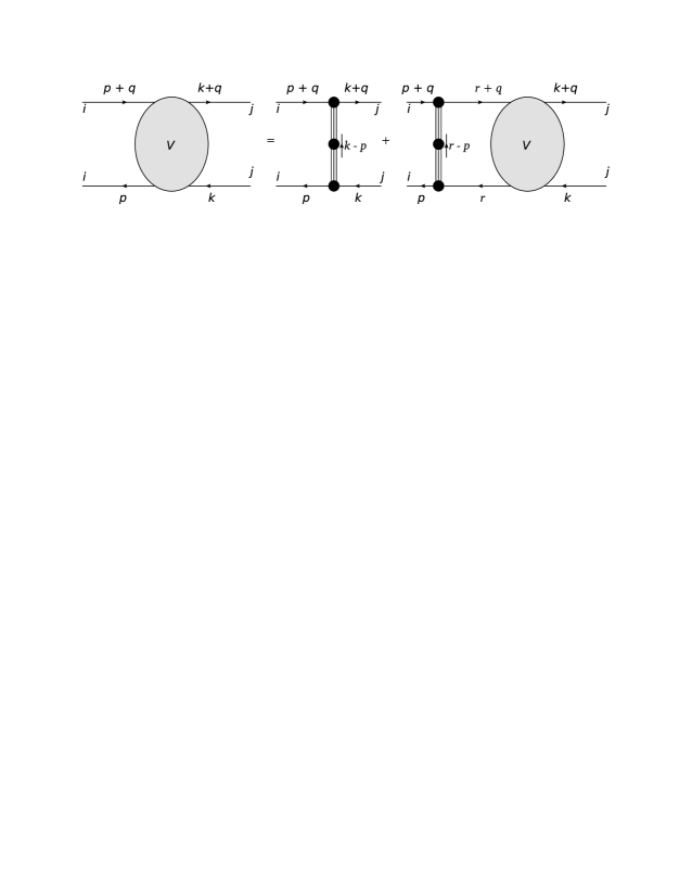
Figure 5: A diagrammatic depiction of the integral equation obeyed by offshell four point scattering amplitudes. The blob here represents the all orders scattering amplitude while the triple line represents the effective single particle exchange four point interaction between quanta. Here, and in every Feynman diagram in this paper, all momenta flow in the direction of the arrows of the propagators.

According to the labeling of momenta in Fig. 5, $q^{\mu}$ is the three momentum that flows, from left to right in graphs of Fig. 3. $q^{\mu}$ is a ‘constant of motion’ in the sense that if a given ladder diagram has a particular value of $q^{\mu}$ then every sub ladder within the original ladder also has the same value of $q^{\mu}$ (this is not true of the momenta $p$ and $k$ in Fig. 3). This implies that different values of $q^{\mu}$ do not ‘mix’ in the integral equation of Fig. 5. In other words Fig. 5 represents an infinite set of decoupled integral equations; one for every value of $q^{\mu}$. It was pointed out in [5] that the integral equations in Fig. 5 simplifies dramatically when $q^{\pm}=0$. The authors of [5] infact solved the relevant integral equations for the bosonic theory in massless limit. In this paper to find exact formulae for the sum over planar graphs with four external lines with $q^{\pm}=0$ by explicitly solving the integral equations relevant to that case. In the case of the bosonic theory our results are a generalization of those of [5] to nonzero mass The integral equation turns out to be more complicated to solve in the case of the fermionic theory, but we are able to find the exact solution in this case as well.

With exact off shell results in hand, we proceed to evaluate the S-matrices for our problem by taking the appropriate on shell limits. The on shell condition determines the energy of each of the participating particles (in terms of their momenta) upto a sign. Energy and momentum conservation require that two of the external lines have positive energy while the other two have negative energy, leaving a total of six distinct cases. Recalling that external lines with positive energy represent initial states while external lines with negative energy represent final states, it is not difficult to convince oneself that one of these six cases determines the function $T_{S}$, another determines $T_{T}$, two others determine $T_{U_{d}}$, $T_{U_{e}}$ respectively, while the last two processes compute the CPT conjugates of scattering in the $U$-channel. In other words the four different scattering functions introduced, in the previous subsection, are all different limits of the single four point amplitudes determined by the integral equation of Fig. 5.

As we have emphasized above, we have been able to evaluate the off shell four point amplitude only in the special case $q^{\pm}=0$. This technical limitation has different implications for our ability to compute the $S$ matrices in the different channels.

$q^{\mu}$ turns out to be the center of mass 3 momentum for $S$-channel scattering. The condition $q^{\pm}=0$ ensures that the center of mass energy is spacelike; this is impossible for an onshell scattering process. It follows that the technical limitations which restricted us to $q^{\pm}=0$ forbid us from directly computing $S$-channel scattering, a fact that will force us to resort to conjecture in this channel.

In the $T$ and $U$-channels, on the other hand, $q$ represents the 3 momentum transfer between an initial and final particle. As all participating particles have the same mass, the 3 momentum transfer is always spacelike (this is most easily seen in the center of mass frame), there is no barrier to setting $q^{\pm}=0$ in these processes. For an arbitrary $T$ or $U$-channel process, it is always possible to find an inertial frame in which $q^{\pm}=0$. In these channels, in other words, the restriction to $q^{\pm}=0$ is simply a choice of frame. Assuming that the S-matrix for our process is Lorentz invariant, the on shell limits of our off shell four point amplitude completely fix the S-matrix in these channels. We are thus able to report definite results for the scattering matrices in these channels.

3.2 Results in the $U$ and $T$ channels

In this subsection we simply present our final results for $U$ and $T$-channel scattering, separately for the bosonic and the fermionic theories. We first report our results for the bosonic theory. In the $T$-channel (adjoint exchange) we find

$$\begin{split}&T^{B}_{T}(p_{1},p_{2},p_{3},p_{4},k_{B},\lambda_{B},{\tilde{b}}_{4},c_{B})\\ =&E(p_{1},p_{2},p_{3})\frac{4i\pi}{k_{B}}\sqrt{\frac{u~{}t}{s}}\\ &-\frac{4~{}i\pi}{k_{B}}\sqrt{-t}~{}~{}\frac{({\tilde{b}}_{4}-4\pi i\lambda_{B}\sqrt{-t})e^{i\pi\lambda_{B}}+({\tilde{b}}_{4}+4\pi i\lambda_{B}\sqrt{-t})e^{2i\lambda_{B}\tan^{-1}\left(\frac{2|c_{B}|}{\sqrt{-t}}\right)}}{-({\tilde{b}}_{4}-4\pi i\lambda_{B}\sqrt{-t})e^{i\pi\lambda_{B}}+({\tilde{b}}_{4}+4\pi i\lambda_{B}\sqrt{-t})e^{2i\lambda_{B}\tan^{-1}\left(\frac{2|c_{B}|}{\sqrt{-t}}\right)}}~{}~{}\\ =&E(p_{1},p_{2},p_{3})\frac{4i\pi}{k_{B}}\sqrt{\frac{u~{}t}{s}}\\ &-\frac{4~{}i\pi}{k_{B}}\sqrt{-t}~{}~{}\frac{({\tilde{b}}_{4}-4\pi i\lambda_{B}\sqrt{-t})+({\tilde{b}}_{4}+4\pi i\lambda_{B}\sqrt{-t})e^{-2i\lambda_{B}\tan^{-1}\left(\frac{\sqrt{-t}}{2|c_{B}|}\right)}}{-({\tilde{b}}_{4}-4\pi i\lambda_{B}\sqrt{-t})+({\tilde{b}}_{4}+4\pi i\lambda_{B}\sqrt{-t})e^{-2i\lambda_{B}\tan^{-1}\left(\frac{\sqrt{-t}}{2|c_{B}|}\right)}}~{}~{}\\ \end{split}$$ (71)

where we have used

$$\tan^{-1}(x)+\tan^{-1}(\frac{1}{x})=\frac{\pi}{2},~{}~{}\rm{for}~{}~{}x>0$$

and $\tilde{b}_{4}=-b_{4}+2\pi\lambda_{B}^{2}|c_{B}|.$ Here form of the $\tan^{-1}(x)$ is

$$\tan^{-1}x=\frac{1}{2i}\ln\left(\frac{1+ix}{1-ix}\right)$$ (72)

and the domain and the branch cut structure of the function $\tan^{-1}(x)$ are depicted in Fig. 6.

In the special case $b_{4}\to\infty$, $T_{T}$ reduces to

$$\begin{split}T^{B\infty}_{T}(p_{1},p_{2},p_{3},p_{4},k_{B},\lambda_{B},c_{B})=&E(p_{1},p_{2},p_{3})\frac{4i\pi}{k_{B}}\sqrt{\frac{u~{}t}{s}}\\ &-\frac{4~{}i\pi}{k_{B}}\sqrt{-t}~{}~{}\frac{1+e^{-2i\lambda_{B}\tan^{-1}\left(\frac{\sqrt{-t}}{2|c_{B}|}\right)}}{1-e^{-2i\lambda_{B}\tan^{-1}\left(\frac{\sqrt{-t}}{2|c_{B}|}\right)}}~{}~{}.\end{split}$$ (73)

In the $U$-channel we find

$$\begin{split}&T^{B}_{U_{d}}(p_{1},p_{2},p_{3},p_{4},k_{B},\lambda_{B},{\tilde{b}}_{4},c_{B})\\ =&E(p_{1},p_{2},p_{3})\frac{4i\pi}{k_{B}}\sqrt{\frac{s~{}t}{u}}\\ &-\frac{4~{}i\pi}{k_{B}}\sqrt{-t}~{}~{}\frac{({\tilde{b}}_{4}-4\pi i\lambda_{B}\sqrt{-t})+({\tilde{b}}_{4}+4\pi i\lambda_{B}\sqrt{-t})e^{-2i\lambda_{B}\tan^{-1}\left(\frac{\sqrt{-t}}{2|c_{B}|}\right)}}{-({\tilde{b}}_{4}-4\pi i\lambda_{B}\sqrt{-t})+({\tilde{b}}_{4}+4\pi i\lambda_{B}\sqrt{-t})e^{-2i\lambda_{B}\tan^{-1}\left(\frac{\sqrt{-t}}{2|c_{B}|}\right)}}.~{}~{}\\ \end{split}$$ (74)

In the limit $b_{4}\to\infty$ we have

$$\begin{split}T^{B\infty}_{U_{d}}(p_{1},p_{2},p_{3},p_{4},k_{B},\lambda_{B},c_{B})=&E(p_{1},p_{2},p_{3})\frac{4i\pi}{k_{B}}\sqrt{\frac{s~{}t}{u}}\\ &-\frac{4~{}i\pi}{k_{B}}\sqrt{-t}~{}~{}\frac{1+e^{-2i\lambda_{B}\tan^{-1}\left(\frac{\sqrt{-t}}{2|c_{B}|}\right)}}{1-e^{-2i\lambda_{B}\tan^{-1}\left(\frac{\sqrt{-t}}{2|c_{B}|}\right)}}.~{}~{}\end{split}$$ (75)

Finally, the amplitude $T^{B}_{U_{e}}$ is obtained from $T^{B}_{U_{d}}$ simply by interchanging the two initial momenta. The usual symmetry of bosonic amplitudes immediately implies

$$T^{B}_{U_{e}}(p_{1},p_{2},p_{3},p_{4},k_{B},\lambda_{B},b_{4},c_{B})=T^{B}_{U_{d}}(p_{2},p_{1},p_{3},p_{4},k_{B},\lambda_{B},b_{4},c_{B})$$ (76)

with a similar formula for $S^{\infty}_{U_{e}}(p_{1},p_{2},p_{3},p_{4},k_{B},\lambda_{B},c_{B}).$

We now report our results for the fermionic theory. In this case S-matrix in the $T$-channel is given by

$$\begin{split}&T^{F}_{T}(p_{1},p_{2},p_{3},p_{4},k_{F},\lambda_{F},c_{F})\\ =&-E(p_{1},p_{2},p_{3})\frac{4i\pi}{k_{F}}\sqrt{\frac{u~{}t}{s}}\\ &+\frac{4~{}i\pi}{k_{F}}\sqrt{-t}~{}~{}\frac{e^{i\pi\left(\lambda_{F}-{\rm sgn}(m_{F})\right)}+e^{2i\left(\lambda_{F}-{\rm sgn}(m_{F})\right)\tan^{-1}\left(\frac{2|c_{F}|}{\sqrt{-t}}\right)}}{e^{i\pi\left(\lambda_{F}-{\rm sgn}(m_{F})\right)}-e^{2i\left(\lambda_{F}-{\rm sgn}(m_{F})\right)\tan^{-1}\left(\frac{2|c_{F}|}{\sqrt{-t}}\right)}}~{}~{}\\ =&-E(p_{1},p_{2},p_{3})\frac{4i\pi}{k_{F}}\sqrt{\frac{u~{}t}{s}}+\frac{4~{}i\pi}{k_{F}}\sqrt{-t}~{}~{}\frac{1+e^{-2i\left(\lambda_{F}-{\rm sgn}(m_{F})\right)\tan^{-1}\left(\frac{\sqrt{-t}}{2|c_{F}|}\right)}}{1-e^{-2i\left(\lambda_{F}-{\rm sgn}(m_{F})\right)\tan^{-1}\left(\frac{\sqrt{-t}}{2|c_{F}|}\right)}}.~{}~{}\\ \end{split}$$ (77)

In the $U$-channel we find

$$\begin{split}&T_{U_{d}}^{F}(p_{1},p_{2},p_{3},p_{4},k_{F},\lambda_{F},c_{F})\\ =&-\Bigg{(}-E(p_{1},p_{2},p_{3})\frac{4i\pi}{k_{F}}\sqrt{\frac{s~{}t}{u}}\\ &\qquad+\frac{4~{}i\pi}{k_{F}}\sqrt{-t}~{}~{}\frac{e^{i\pi\left(\lambda_{F}-{\rm sgn}(m_{F})\right)}+e^{2i\left(\lambda_{F}-{\rm sgn}(m_{F})\right)\tan^{-1}\left(\frac{2|c_{F}|}{\sqrt{-t}}\right)}}{e^{i\pi\left(\lambda_{F}-{\rm sgn}(m_{F})\right)}-e^{2i\left(\lambda_{F}-{\rm sgn}(m_{F})\right)\tan^{-1}\left(\frac{2|c_{F}|}{\sqrt{-t}}\right)}}\Bigg{)}~{}~{}\\ &=-\Bigg{(}-E(p_{1},p_{2},p_{3})\frac{4i\pi}{k_{F}}\sqrt{\frac{s~{}t}{u}}+\frac{4~{}i\pi}{k_{F}}\sqrt{-t}~{}~{}\frac{1+e^{-2i\left(\lambda_{F}-{\rm sgn}(m_{F})\right)\tan^{-1}\left(\frac{\sqrt{-t}}{2|c_{F}|}\right)}}{1-e^{-2i\left(\lambda_{F}-{\rm sgn}(m_{F})\right)\tan^{-1}\left(\frac{\sqrt{-t}}{2|c_{F}|}\right)}}\Bigg{)}.\end{split}$$ (78)

Finally, the usual symmetry for fermionic amplitudes immediately implies that

$$T^{F}_{U_{e}}(p_{1},p_{2},p_{3},p_{4},k_{F},\lambda_{F},c_{F})=-T^{F}_{U_{d}}(p_{2},p_{1},p_{3},p_{4},k_{F},\lambda_{F},c_{F}).$$ (79)

As we have mentioned earlier in this introduction, in the limit $b_{4}\to\infty$, the bosonic theory studied in this paper has been conjectured to be dual to the fermionic theory, when the parameters of the two theories are related by (14). Our results for the scattering amplitudes reported above are in perfect agreement with this conjecture. In particular it may be verified that, provided the inequality (15) is obeyed, the bosonic and fermionic S-matrices (including the identity pieces, see subsections 2.3 and 2.4)

$$\begin{split}&{\bf S}^{B\infty}_{T}(p_{1},p_{2},p_{3},p_{4},-k_{F},\lambda_{F}-{\rm sgn}(\lambda_{F}),c_{F})={\bf S}^{F}_{T}(p_{1},p_{2},p_{3},p_{4},k_{F},\lambda_{F},c_{F}),\\ &{\bf S}^{B\infty}_{U_{d}}(p_{1},p_{2},p_{3},p_{4},-k_{F},\lambda_{F}-{\rm sgn}(\lambda_{F}),c_{F})=-{\bf S}^{F}_{U_{d}}(p_{1},p_{2},p_{3},p_{4},k_{F},\lambda_{F},c_{F}),\\ &{\bf S}^{B\infty}_{U_{e}}(p_{1},p_{2},p_{3},p_{4},-k_{F},\lambda_{F}-{\rm sgn}(\lambda_{F}),c_{F})={\bf S}^{F}_{U_{e}}(p_{1},p_{2},p_{3},p_{4},k_{F},\lambda_{F},c_{F}),\\ &{\bf S}^{B\infty}_{U_{s}}(p_{1},p_{2},p_{3},p_{4},-k_{F},\lambda_{F}-{\rm sgn}(\lambda_{F}),c_{F})={\bf S}^{F}_{U_{a}}(p_{1},p_{2},p_{3},p_{4},k_{F},\lambda_{F},c_{F}),\\ &{\bf S}^{B\infty}_{U_{a}}(p_{1},p_{2},p_{3},p_{4},-k_{F},\lambda_{F}-{\rm sgn}(\lambda_{F}),c_{F})={\bf S}^{F}_{U_{s}}(p_{1},p_{2},p_{3},p_{4},k_{F},\lambda_{F},c_{F}).\\ \end{split}$$ (80)

3.3 A conjecture for identity exchange and modified crossing symmetry

In the case of the bosonic theory we conjecture that $S$ matrix in the $S$-channel is given by

$${\bf S}_{S}^{B}=\cos(\pi\lambda_{B})I(p_{1},p_{2},p_{3},p_{4})+i\frac{\sin(\pi\lambda_{B})}{\pi\lambda_{B}}T_{S}^{trial}$$ (81)

where $T_{S}^{trial}$ is the $S$-channel S-matrix obtained from analytic continuation of the $T$ or $U$-channel results using the usual rules of ‘naive’ crossing symmetry, and is given by

$$\begin{split}T_{S}^{trial}=&\left(\pi\lambda_{B}\right)4~{}i\sqrt{s}E(p_{1},p_{2},p_{3})\sqrt{\frac{u}{t}}\\ &+\left(\pi\lambda_{B}\right)4\sqrt{s}\left(\frac{\left(4\pi\lambda_{B}\sqrt{s}+\widetilde{b}_{4}\right)+e^{i\pi\lambda_{B}}\left(-4\pi\lambda_{B}\sqrt{s}+\widetilde{b}_{4}\right)\left(\frac{\frac{1}{2}+\frac{c_{B}}{\sqrt{s}}}{\frac{1}{2}-\frac{c_{B}}{\sqrt{s}}}\right)^{\lambda_{B}}}{\left(4\pi\lambda_{B}\sqrt{s}+\widetilde{b}_{4}\right)-e^{i\pi\lambda_{B}}\left(-4\pi\lambda_{B}\sqrt{s}+\widetilde{b}_{4}\right)\left(\frac{\frac{1}{2}+\frac{c_{B}}{\sqrt{s}}}{\frac{1}{2}-\frac{c_{B}}{\sqrt{s}}}\right)^{\lambda_{B}}}\right).\\ \end{split}$$ (82)

In the limit $b_{4}\to\infty,$ $T_{S}^{trial}$ simplifies to

$$T_{S}^{trial}=\left(\pi\lambda_{B}\right)4~{}i\sqrt{s}\left(E(p_{1},p_{2},p_{3})\sqrt{\frac{u}{t}}+\left(\frac{1+e^{i\pi\lambda_{B}}\left(\frac{\frac{1}{2}+\frac{c_{B}}{\sqrt{s}}}{\frac{1}{2}-\frac{c_{B}}{\sqrt{s}}}\right)^{\lambda_{B}}}{1-e^{i\pi\lambda_{B}}\left(\frac{\frac{1}{2}+\frac{c_{B}}{\sqrt{s}}}{\frac{1}{2}-\frac{c_{B}}{\sqrt{s}}}\right)^{\lambda_{B}}}\right)\right).\\$$ (83)

In a similar manner we expect that the fermionic S-matrix is given by

$$\begin{split}S_{S}^{F}&=\cos(\pi\lambda_{F})I(p_{1},p_{2},p_{3},p_{4})+i\frac{\sin(\pi\lambda_{F})}{\pi\lambda_{F}}T_{F}^{trial}\\ &=\sin(\pi\lambda_{F})\Bigg{(}4E(p_{1},p_{2},p_{3})\sqrt{\frac{s~{}t}{u}}+4\sqrt{s}~{}~{}\frac{1+e^{-2i\left(\lambda_{F}-{\rm sgn}(m_{F})\right)\tan^{-1}\left(\frac{\sqrt{s}}{2|c_{F}|}\right)}}{1-e^{-2i\left(\lambda_{F}-{\rm sgn}(m_{F})\right)\tan^{-1}\left(\frac{\sqrt{s}}{2|c_{F}|}\right)}}~{}~{}\Bigg{)}\\ &+\cos(\pi\lambda_{F})I(p_{1},p_{2},p_{3},p_{4}).\end{split}$$ (84)

It follows from (81), (84) and the results of the previous subsection the fermionic and bosonic $S$-channel $S$ matrices map to each other under duality upto an overall minus sign (recall that overall phases in an S-matrix are unobservable and so unimportant).

4 Scattering in the scalar theory

In this section we compute the four point scattering amplitude in the theory of fundamental bosons coupled to Chern-Simons theory. Very briefly we integrate out the gauge boson to obtain an offshell effective four boson term in the quantum effective action for our theory, given by

$$\frac{1}{2}\int\frac{d^{3}p}{(2\pi)^{3}}\frac{d^{3}k}{(2\pi)^{3}}\frac{d^{3}q}{(2\pi)^{3}}V(p,k,q){\phi}_{i}(p+q){\bar{\phi}}^{j}(-(k+q)){\bar{\phi}}^{i}(-p)\phi_{j}(k).$$ (85)

We then take an appropriate on shell limit to evaluate the S-matrix.

4.1 Integral equation for off shell four point amplitude

As explained in the previous section, $V(p,k,q)$ obeys the integral equation depicted in Fig 5. In formulas

$$\begin{split}V(p,k,q)&=V_{0}(p,k,q)-i\int\frac{d^{3}r}{(2\pi)^{3}}V(p,r,q_{3})\frac{NV_{0}(r,k,q_{3})}{\left(r^{2}+c_{B}^{2}-i\epsilon\right)\left((r+q)^{2}+c_{B}^{2}-i\epsilon\right)},\\ V(p,k,q)&=V_{0}(p,k,q)-i\int\frac{d^{3}r}{(2\pi)^{3}}V_{0}(p,r,q_{3})\frac{NV(r,k,q_{3})}{\left(r^{2}+c_{B}^{2}-i\epsilon\right)\left((r+q)^{2}+c_{B}^{2}-i\epsilon\right)},\end{split}$$ (86)

where the ‘one particle’ amplitude $V_{0}$ is given by the sum of graphs in Fig. 4. Summing these graphs (see Appendix D.1 for details) we find

$$\begin{split}NV_{0}(p,k,q_{3})&=-4\pi i\lambda_{B}q_{3}\frac{(k+p)_{-}}{(k-p)_{-}}+\widetilde{b}_{4},\\ \widetilde{b}_{4}&=2\pi\lambda_{B}^{2}c_{B}-b_{4}.\end{split}$$ (87)

Here

$$d^{3}r=dr^{0}dr^{1}dr^{3},~{}~{}~{}k_{\pm}=\frac{\pm k_{0}+k_{1}}{\sqrt{2}}.~{}~{}~{}$$ (88)

(87) is actually ambiguous as stated. The first term on the RHS of (87) is proportional to $\frac{1}{(k-p)_{-}}$: the gauge boson propagator in lightcone gauge. This term is ill defined when $k_{-}=p_{-}$, a point that lies on the integration contour on the RHS of (34).

The reason that the gauge boson has a codimension two singularity in momentum space is that the choice of lightcone gauge, $A_{-}=0$, leaves unfixed the residual gauge transformations that depend only on $x^{+}$ and $x^{3}$. In this paper we resolve this ambiguity of the propagator at $p_{-}=0$ with the ‘Feynman’ prescription

$$\frac{1}{p_{-}}\rightarrow\frac{p_{+}}{p_{+}p_{-}-i\epsilon}.$$ (89)

We adopt this prescription for several reasons.

• 1. It is the only resolution of the singularity of the gauge propagator that permits continuation to Euclidean space. It therefore appears to be the only resolution of the singularity that can make contact with all the beautiful Euclidean results of [1, 2, 7, 3, 4, 8, 9, 10, 5].

• 2. Its use leads to sensible results with no unphysical divergences.  

• 3. In special cases, results obtained by use of this prescription turn out to agree with results in the covariant Landau gauge (see subsection 5 below).

Of course the pragmatic reasons spelt out above are ultimately unsatisfactory; we would like eventually to have a justification of this prescription on physical grounds (such a justification would presumably involve a careful accounting for the unfixed gauge symmetry of the problem). However we leave this potentially subtle exercise to future work.

4.2 Euclidean continuation

In order to solve the integral equation (86) we will find it convenient to use a standard maneuver to ‘continue this equation to Euclidean space’. Operationally, the procedure is to define a Euclidean amplitude via $V^{E}(p^{0},k^{0})=V(ip^{0},ik^{0})$. Once the amplitude $V^{E}$ has been solved for, the amplitude of real physical interest, $V$, is obtained by the inverse relation

$$V(p^{0},k^{0})=V^{E}(-ip^{0},-ik^{0}).$$

Even though the method of Euclidean continuation is standard in the study of scattering amplitudes, for completeness we recall the justification of this method, in the context of our problem, in Appendix D.2. We emphasize that this procedure is valid only when the singularities of all propagators in the Lorentzian problem are resolved by the Feynman $i\epsilon$ prescription. This is one of the main reasons we adopted the $i\epsilon$ prescription of (89) above.

The Euclidean continuation of the scattering amplitude obeys the integral equation

$$\begin{split}V^{E}(p,k,q)&=V^{E}_{0}(p,k,q)+\int\frac{d^{3}r}{(2\pi)^{3}}V_{0}^{E}(p,r,q_{3})\frac{NV^{E}(r,k,q_{3})}{\left(r^{2}+c_{B}^{2}\right)\left((r+q)^{2}+c_{B}^{2}\right)}\\ V^{E}(p,k,q)&=V^{E}_{0}(p,k,q)+\int\frac{d^{3}r}{(2\pi)^{3}}V^{E}(p,r,q_{3})\frac{NV^{E}_{0}(r,k,q_{3})}{\left(r^{2}+c_{B}^{2}\right)\left((r+q)^{2}+c_{B}^{2}\right)}\\ NV^{E}_{0}(p,k,q_{3})&=-4\pi i\lambda_{B}q_{3}\frac{(k+p)_{-}}{(k-p)_{-}}+\widetilde{b}_{4}\\ \end{split}$$ (90)

where

$$d^{3}r=dr^{0}dr^{1}dr^{3},~{}~{}~{}k_{\pm}=\frac{k_{1}\pm ik_{0}}{\sqrt{2}}.~{}~{}~{}$$ (91)

Note, in particular, that $k_{\pm}$ are now complex conjugates of each other. Below we will sometimes use the notation

$$k_{s}^{2}=2k_{+}k_{-}=k_{1}^{2}+k_{0}^{2}.$$ (92)

4.3 Solution of the Euclidean integral equation

The integral equation (90) may be solved in a completely systematic manner. We have presented a detailed derivation of our solution of this equation in Appendix D.3. In this subsection we simply quote our final results.

Our solution takes the form

$$NV=e^{-2i\lambda_{B}\left(\tan^{-1}\left(\frac{2(a(k))}{q_{3}}\right)-\tan^{-1}\left(\frac{2(a(p))}{q_{3}}\right)\right)}\left(4\pi i\lambda_{B}q_{3}\frac{p_{-}+k_{-}}{p_{-}-k_{-}}+j(q_{3},\lambda_{B})\right)$$ (93)

where

$$a(p)=\sqrt{2p_{+}p_{-}+c_{B}^{2}}$$ (94)

and

$$j(q_{3},\lambda_{B})={4\pi i\lambda_{B}q_{3}}\left(\frac{\left(4\pi i\lambda_{B}q_{3}+\widetilde{b}_{4}\right)e^{2i\lambda_{B}\tan^{-1}\left(\frac{2c_{B}}{q_{3}}\right)}+\left(-4\pi i\lambda_{B}q_{3}+\widetilde{b}_{4}\right)e^{\pi i\lambda_{B}{\rm sgn}(q_{3})}}{\left(4\pi i\lambda_{B}q_{3}+\widetilde{b}_{4}\right)e^{2i\lambda_{B}\tan^{-1}\left(\frac{2c_{B}}{q_{3}}\right)}-\left(-4\pi i\lambda_{B}q_{3}+\widetilde{b}_{4}\right)e^{\pi i\lambda_{B}{\rm sgn}(q_{3})}}\right).$$ (95)

It is not difficult to verify that

$$j(q_{3},\lambda_{B})=j(-q_{3},\lambda_{B})=j(q_{3},-\lambda_{B})=j(-q_{3},-\lambda_{B})=j(|q_{3}|,|\lambda_{B}|).$$ (96)

In other words, $j$ is an even function of $q_{3}$ and $\lambda_{B}$ separately. It follows in particular that

$$j(q,\lambda_{B})={4\pi i\lambda_{B}|q|}\left(\frac{\left(4\pi i\lambda_{B}|q|+\widetilde{b}_{4}\right)e^{2i\lambda_{B}\tan^{-1}\left(\frac{2c_{B}}{|q|}\right)}+\left(-4\pi i\lambda_{B}|q|+\widetilde{b}_{4}\right)e^{\pi i\lambda_{B}}}{\left(4\pi i\lambda_{B}|q|+\widetilde{b}_{4}\right)e^{2i\lambda_{B}\tan^{-1}\left(\frac{2c_{B}}{|q_{3}|}\right)}-\left(-4\pi i\lambda_{B}|q|+\widetilde{b}_{4}\right)e^{\pi i\lambda_{B}}}\right).$$ (97)

This formula may be rewritten as follows. Let us define

$$\begin{split}H(q)&=\int\frac{d^{3}r}{(2\pi)^{3}}\frac{1}{\left(r^{2}+c_{B}^{2}\right)\left((r+q)^{2}+c_{B}^{2}\right)}=\left(-\frac{\tan^{-1}\left(\frac{2c_{B}}{|q_{3}|}\right)}{4\pi|q_{3}|}+\frac{1}{8|q_{3}|}\right)\\ &=\frac{\tan^{-1}\left(\frac{|q_{3}|}{2c_{B}}\right)}{4\pi|q_{3}|}\\ &=\frac{1}{8\pi i|q|}\ln\left(\frac{\frac{1}{2}+\frac{c_{B}}{iq}}{-\frac{1}{2}+\frac{c_{B}}{iq}}\right).\end{split}$$ (98)

Here to get the last line, we have used the formula (72). $H(q)$ is simply the one loop four boson scattering amplitude in $\phi^{4}$ theory. In terms of this function we have

$$j(q)={4\pi i\lambda_{B}|q|}\left(\frac{\left(4\pi i\lambda_{B}|q|+\widetilde{b}_{4}\right)+\left(-4\pi i\lambda_{B}|q|+\widetilde{b}_{4}\right)e^{8i\pi\lambda_{B}|q|H(q)}}{\left(4\pi i\lambda_{B}|q|+\widetilde{b}_{4}\right)-\left(-4\pi i\lambda_{B}|q|+\widetilde{b}_{4}\right)e^{8i\pi\lambda_{B}|q|H(q)}}\right).$$ (99)

Using the last line in (98) $j(q)$ may also be rewritten as

$$j(q)=4\pi iq\lambda_{B}\left(\frac{\left(4\pi iq\lambda_{B}+\widetilde{b}_{4}\right)+\left(-4\pi iq\lambda_{B}+\widetilde{b}_{4}\right)\left(\frac{\frac{1}{2}+\frac{c_{B}}{iq}}{-\frac{1}{2}+\frac{c_{B}}{iq}}\right)^{\lambda_{B}}}{\left(4\pi iq\lambda_{B}+\widetilde{b}_{4}\right)-\left(-4\pi iq\lambda_{B}+\widetilde{b}_{4}\right)\left(\frac{\frac{1}{2}+\frac{c_{B}}{iq}}{-\frac{1}{2}+\frac{c_{B}}{iq}}\right)^{\lambda_{B}}}\right).$$ (100)

4.3.1 Transformation under parity

While parity transformations are not a symmetry of the bosonic theory, the simultaneous action of a parity transformation and the flip in the sign of $k_{B}$ (or $\lambda_{B}$) is symmetry of this theory. Every physical quantity in this theory must, therefore, transform in a suitably ‘nice’ way under the combined action of these two transformations.

The off shell Greens function computed in the previous subsection is not physical as it is not gauge invariant, and so need not transform ‘nicely’ under parity operations. Indeed it is easily verified by inspection that the amplitude $V$ is left invariant by a reflection in the $3$ direction accompanied by a flip in the sign of $\lambda_{B}$. However the combined operation of a flip in the sign of $\lambda_{B}$ and a reflection in either the $0$ or $1$ directions is not an invariance of this amplitude. The reason for this asymmetry is that reflections in the 3 direction are the only parity transformations that commute with the choice of light cone gauge (for instance a reflection in the $1$ direction changes the gauge $A_{-}=0$ to $A_{+}=0$. ).

As we will see below, the physical $S$ matrix indeed enjoys the full parity symmetry expected of this theory.

4.4 Analytic continuation of $j(q)$

In our study of $S$-channel scattering later in this paper we will need to continue the function $j(q)$ to $q^{2}=-s$. This analytic continuation is achieved by setting $q=\lim_{\alpha\to\frac{\pi}{2}}e^{-i\alpha\frac{\pi}{2}}\sqrt{s}$ or equivalently by setting

$$q\rightarrow-i\left(\sqrt{s}+i\epsilon\right)$$

The precise analytic continuation we will use is the following. We will take the function $j(q)$ to be defined by (99), where $H(q)$ is defined by (98). The function $\tan^{-1}(x)$ that appears in some versions of the definition of $H(q)$ is taken to have the analytic structure depicted in Fig. 6

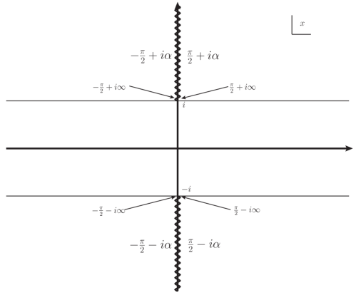
Figure 6: Branch cut structure of the function $\tan^{-1}x$. $\alpha$ is a real function of x along the branch cut which vanishes at infinities and becomes $\infty$ at $|Im(x)|=1$.

The function $H(q)$ (see (98) ) analytically continues to $H^{M}(\sqrt{s})$

$$\begin{split}H^{M}(\sqrt{s})=&-i\int\frac{d^{3}r}{(2\pi)^{3}}\frac{1}{\left(r^{2}+c_{B}^{2}-i\epsilon\right)\left((r+q)^{2}+c_{B}^{2}-i\epsilon\right)}\\ =&\frac{1}{8\pi\sqrt{s}}\ln\left(\frac{\frac{1}{2}+\frac{c_{B}}{\sqrt{s+i\epsilon}}}{-\frac{1}{2}+\frac{c_{B}}{\sqrt{s+i\epsilon}}}\right).\end{split}$$ (102)

For $\sqrt{s}<2c_{B}$, the factors of $i\epsilon$ make no difference in the formula (102) and may simply be dropped. When $\sqrt{s}>2c_{B}$, the factors of $i\epsilon$ choose out the branch of logarithmic function and we have

$$H^{M}(\sqrt{s})=\begin{cases}\frac{1}{8\pi\sqrt{s}}\ln\left(\frac{\frac{1}{2}+\frac{c_{B}}{\sqrt{s}}}{-\frac{1}{2}+\frac{c_{B}}{\sqrt{s}}}\right)&(\sqrt{s}<2c_{B})\\ \frac{1}{8\pi\sqrt{s}}\left(\ln\left(\frac{\frac{1}{2}+\frac{c_{B}}{\sqrt{s}}}{\frac{1}{2}-\frac{c_{B}}{\sqrt{s}}}\right)+i\pi\right)&(\sqrt{s}>2c_{B})\end{cases}.$$ (103)

It follows, in particular, that

$$-i\left(H(\sqrt{s}-H^{*}(\sqrt{s})\right)=\frac{\theta(\sqrt{s}-2c_{B})}{4\pi\sqrt{s}}.$$ (104)

Let $j^{M}$ denote the analytic continuation of $j(q)$. It follows that

$$\begin{split}j^{M}(\sqrt{s})=&(\pi\lambda_{B})(4\sqrt{s})\left(\frac{\left(4\pi\lambda_{B}\sqrt{s}+\widetilde{b}_{4}\right)+\left(-4\pi\lambda_{B}\sqrt{s}+\widetilde{b}_{4}\right)e^{8\pi\lambda_{B}\sqrt{s}H^{M}(\sqrt{s})}}{\left(4\pi\lambda_{B}\sqrt{s}+\widetilde{b}_{4}\right)-\left(-4\pi\lambda_{B}\sqrt{s}+\widetilde{b}_{4}\right)e^{8\pi\lambda_{B}\sqrt{s}H^{M}(\sqrt{s})}}\right),\\ j^{M}(\sqrt{s})=&\begin{cases}(\pi\lambda_{B})(4\sqrt{s})\left(\frac{\left(4\pi\lambda_{B}\sqrt{s}+\widetilde{b}_{4}\right)+\left(-4\pi\lambda_{B}\sqrt{s}+\widetilde{b}_{4}\right)\left(\frac{\frac{1}{2}+\frac{c_{B}}{\sqrt{s}}}{-\frac{1}{2}+\frac{c_{B}}{\sqrt{s}}}\right)^{\lambda_{B}}}{\left(4\pi\lambda_{B}\sqrt{s}+\widetilde{b}_{4}\right)-\left(-4\pi\lambda_{B}\sqrt{s}+\widetilde{b}_{4}\right)\left(\frac{\frac{1}{2}+\frac{c_{B}}{\sqrt{s}}}{-\frac{1}{2}+\frac{c_{B}}{\sqrt{s}}}\right)^{\lambda_{B}}}\right),&(\sqrt{s}<2c_{B})\\ (\pi\lambda_{B})(4\sqrt{s})\left(\frac{\left(4\pi\lambda_{B}\sqrt{s}+\widetilde{b}_{4}\right)+e^{i\pi\lambda_{B}}\left(-4\pi\lambda_{B}\sqrt{s}+\widetilde{b}_{4}\right)\left(\frac{\frac{1}{2}+\frac{c_{B}}{\sqrt{s}}}{\frac{1}{2}-\frac{c_{B}}{\sqrt{s}}}\right)^{\lambda_{B}}}{\left(4\pi\lambda_{B}\sqrt{s}+\widetilde{b}_{4}\right)-e^{i\pi\lambda_{B}}\left(-4\pi\lambda_{B}\sqrt{s}+\widetilde{b}_{4}\right)\left(\frac{\frac{1}{2}+\frac{c_{B}}{\sqrt{s}}}{\frac{1}{2}-\frac{c_{B}}{\sqrt{s}}}\right)^{\lambda_{B}}}\right),&(\sqrt{s}>2c_{B})\end{cases}\end{split}$$ (105)

4.5 Poles of the functions $j(q)$ and $j^{M}(\sqrt{s})$

In this subsection we will analyze the conditions under which the functions $j(q)$ and $j^{M}(\sqrt{s})$ have poles for real values of their arguments. The conditions are most conveniently presented in terms of inequalities on $b_{4}$ for fixed values of all other parameters.

Substituting $\widetilde{b}_{4}=2\pi\lambda_{B}^{2}c_{B}-b_{4}$ in the formulas (105) and (100) we can see that for $b_{4}>-2\pi\lambda_{B}c_{B}(4-\lambda_{B})$ neither of the functions above has a pole at real values of its argument. When $-2\pi\lambda_{B}c_{B}(4-\lambda_{B})\geq b_{4}\geq-2\pi c_{B}(4-\lambda_{B}^{2})$ the function $j^{M}$ has a pole, but $j$ has no pole. At the upper end of this interval the pole occurs at $\sqrt{s}=2c_{B}$. At the lower end of this interval the pole value is $\sqrt{s}=0$. For $b_{4}\leq-2\pi c_{B}(4-\lambda_{B}^{2})$, $j^{M}(\sqrt{s})$ has no real poles, but the function $j(q)$ develops a pole. This pole starts out at $q=0$ and migrates to $q=\infty$ as $b_{4}\to-\infty$.

A pole in the function $j^{M}(\sqrt{s})$ at $s=s_{B}$ signals the presence of a particle - antiparticle bound state in the singlet channel. As we have seen above, bound states exist only for $b_{4}$ less than a certain minimum value. We will now explain how this result fits with physical intuition; let us first focus on the special case $\lambda_{B}=0$. In this case poles exist for $b_{4}\leq 0$. In the non-relativistic limit a term $+\int b_{4}\frac{({\bar{\phi}}\phi)^{2}}{2N}$ in the Minkowskian action represents a negative (attractive) delta function interaction between particles and antiparticles when $b_{4}>0$. It seems plausible that such an attractive potential could support a bound state, as appears to be the case. Clearly the binding energy of this system is proportional to $b_{4}$, and so goes to zero in the limit $b_{4}\to 0$. In other words we should expect the mass of the bound state to be given precisely by $2c_{B}$ at $b_{4}=0$, exactly as we find. As $b_{4}$ decreases we should expect the binding energy to increase, i.e. for the bound state energy to decrease, exactly as we find. Above a critical value of $c_{B}$ we find above that the binding energy is so large that the bound state energy vanishes. At even lower values of $b_{4}$ the vacuum is unstable as it is energetically favorable for particle - antiparticle pairs to spontaneously bubble out of the vacuum. This instability is, presumably, signalled by the appearance of the tachyonic pole in $b_{4}$. The instability of the vacuum also seems reasonable from the viewpoint of quantum field theory; a large negative value of $b_{4}$ the classical scalar potential is unbounded from below; plausibly the same is true of the exact potential in the quantum effective action in this regime.

The pattern is very similar at nonzero $\lambda_{B}$; though the precise values of the critical values for $b_{4}$ shift around. Apparently the anyonic interaction in the singlet channel renormalizes the effective interaction of the theory.

Note that bound states do not exist in the limit $b_{4}\to\infty$, the limit in which the bosonic theory is dual to the fermionic theory.

It would be interesting to flesh out the qualitative discussion presented in this subsection. Near the threshold of bound state formation the interacting particles are approximately non-relativistic, so it may be possible to reproduce the pole mass in this regime by solving a Schrodinger equation. We leave this to future work.

4.6 Various limits of the function $j(q)$.

The explicit form of the function $j(q)$ (here $q=\sqrt{|q_{3}|^{2}}$) is one of the principal computational results of this section. $j(q)$ has the dimensions of mass. It is a function of one dimensionless variable $\lambda_{B}$, and three quantities of mass dimension 1; $q$, $c_{B}$ and $b_{4}$. It follows that $j$ takes the form $j=qh(x,y,\lambda_{B})$ where

$$x=\frac{q}{2c_{B}},~{}~{}~{}y=\frac{q}{b_{4}}.$$ (106)

In this subsection we study the behavior of the function $j$ at extreme values of its three dimensionless arguments.

4.6.1 Large $b_{4}$ limit

When $|b|_{4}\gg\lambda_{B}q$ (i.e. when $\lambda_{B}y\ll 1$) the function $j(q)$ simplifies to

$$j(q_{3},\lambda_{B})={4\pi i\lambda_{B}|q_{3}|}\left(\frac{1+e^{8i\pi\lambda_{B}|q_{3}|H(q)}}{1-e^{8i\pi\lambda_{B}|q_{3}|H(q)}}\right)=-4\pi i\lambda_{B}|q_{3}|\left(\frac{1+e^{-2i\lambda_{B}\tan^{-1}\left(\frac{|q_{3}|}{2c_{B}}\right)}}{1-e^{-2i\lambda_{B}\tan^{-1}\left(\frac{|q_{3}|}{2c_{B}}\right)}}\right).$$ (107)

4.6.2 Small $\lambda_{B}$

The function $j$ may be expanded in a Taylor series in $\lambda_{B}$ at fixed values of $x$ and $y$. We find

$$\begin{split}j&=\frac{-b_{4}}{1+b_{4}H(q)}-\frac{16\pi^{2}\lambda_{B}^{2}q_{3}^{2}}{3b_{4}}\left(\frac{1}{\left(b_{4}H(q)+1\right){}^{2}}-b_{4}H(q)-1\right)+{\cal O}(\lambda_{B}^{4}).\end{split}$$ (108)

The limits $\lambda_{B}\to 0$ and $b_{4}\to\infty$ (i.e $\lambda_{B}\to 0$ and $y\to 0$ at fixed $x$ ) commute, so one may obtain the small $\lambda_{B}$ expansion of (107) by simply setting $b_{4}\to\infty$ in (108).

Note that, in the strict $\lambda_{B}\to 0$ limit,

$$\begin{split}&\lim_{\lambda_{B}\to 0}NV(p,k,q^{3})=\lim_{\lambda_{B}\to 0}j(q_{3})=\frac{-b_{4}}{1+b_{4}\frac{\tan^{-1}\left(\frac{|q_{3}|}{2c_{B}}\right)}{4\pi|q_{3}|}}=\frac{-b_{4}}{1+H(q_{3})b_{4}}.\end{split}$$ (109)

(109) is the well known result for the off shell amplitude in large $N$ $\phi^{4}$ theory. It is easily verified by directly solving the integral equation (90) at $\lambda_{B}=0$.

4.6.3 The limit $|\lambda_{B}|\to 1$

The expression for $j(q)$ simplifies somewhat in the limit $\lambda_{B}\to 1$. The simplification is especially dramatic if we also take the limit $b_{4}\to\infty$. In the combined limit $y\to 0$ and $\lambda_{B}\to 1$ (the order of limits does not matter) we have

$$\begin{split}j(q)=&{4\pi iq}\frac{e^{i\tan^{-1}\left(\frac{2c_{B}}{q}\right)}-e^{-i\tan^{-1}\left(\frac{2c_{B}}{q}\right)}}{e^{i\tan^{-1}\left(\frac{2c_{B}}{q}\right)}+e^{-i\tan^{-1}\left(\frac{2c_{B}}{q}\right)}}\\ =&{4\pi iq}(i)\tan\left(\tan^{-1}\left(\frac{2c_{B}}{q}\right)\right)\\ =&-8\pi c_{B}.\end{split}$$ (110)

4.6.4 The ultra-relativistic limit

If $c_{B}$ and $b_{4}$ are held fixed while $\sqrt{-t}$ is taken to infinity (this is the case, for instance, in fixed angle high energy scattering in the $U$ and $T$-channels, see below) , we take $x$ and $y$ to infinity at fixed $\lambda_{B}$ and $j$ simplifies to

$$j(q)=4\pi q\lambda_{B}\tan\frac{\pi\lambda_{B}}{2}.$$ (111)

The ultra relativistic limit does not commute with the limit $b_{4}\to\infty$. If $b_{4}$ is taken to $\infty$ first and $q\to\infty$ next then we work with $y\to 0$, $x\to\infty$ at fixed $\lambda_{B}$ and find

$$j(q)=-4\pi\lambda_{B}q\cot\left(\frac{\pi\lambda_{B}}{2}\right).$$ (112)

The ultra relativistic limit also does not commute with the limit $\lambda_{B}\to 0$. At $\lambda_{B}=0$ the function $j(q)$ tends to a constant proportional to $b_{4}$. Physically this is we have a dimensionless coupling constant at nonzero $\lambda_{B}$, but only a dimensionful coupling constant at any finite $\lambda_{B}$; at zero lambda the theory is very weakly coupled at high energies, and receives contributions only from tree level graphs.

4.6.5 The massless limit

If $c_{B}$ is taken to zero at fixed $b_{4},\lambda_{B}$ and $q$ (i.e. if $x$ is taken to infinity at fixed $y$ and $\lambda_{B}$) then $j$ simplifies to the rational function

$$j(q)={4\pi\lambda_{B}q}\left(\frac{4\pi\lambda_{B}\sin\left(\frac{\pi\lambda_{B}}{2}\right)q+{\tilde{b}}_{4}\cos\left(\frac{\pi\lambda_{B}}{2}\right)}{4\pi\lambda_{B}\cos\left(\frac{\pi\lambda_{B}}{2}\right)q-{\tilde{b}_{4}}\sin\left(\frac{\pi\lambda_{B}}{2}\right)}\right).$$ (113)

The massless limit commutes with the limit $b_{4}\to\infty$. In this limit (113) reduces to (112).

4.6.6 The non-relativistic limit in the $U$ and $T$-channels

As we will see below, the non-relativistic limit in the $U$ and $T$-channels is obtained by taking $c_{B}$ to infinity at fixed $q$. In other words, this limit is obtained by taking $x$ to zero at fixed $\lambda_{B}$ and $y$. In this limit $2i\lambda_{B}\tan^{-1}\left(\frac{2c_{B}}{q_{3}}\right)$ in (97) reduces to $\pi i\lambda_{B}$ and we have

$$j(\sqrt{-t})={\tilde{b}_{4}}.$$ (114)

In this limit, in other words, the function $j$ receives contributions only from tree level scattering with the effective four point coupling ${\tilde{b}}_{4}$ in this limit. No genuine loop diagrams contribute to $T$ and $U$-channel scattering in this limit.

If we first take $b_{4}\to\infty$ and then take the non-relativistic limit we find

$$j(q)=-8\pi c_{B}$$ (115)

As (114) and (115) both tend to infinity in the combined non-relativistic and $b_{4}\to\infty$ limit, the reader may find herself tempted to conclude that the non-relativistic and $b_{4}\to\infty$ commute. This conclusion is, infact, slightly misplaced. As we have emphasized in section 2.6, the true dynamical information in the non-relativistic limit lies in the function

$$h=-\frac{j}{8ic_{B}}$$

which is derived from (54). The correct interpretation of the results of this subsection are that the function $h$ vanishes in the non-relativistic limit at fixed $b_{4}$, but reduces to a $\lambda_{B}$ independent numerical constant if $b_{4}$ is first taken to infinity.

4.7 The non-relativistic limit in the $S$-channel

As we will see below, the function relevant for scattering in the $S$-channel is the analytically continued function $j^{M}(\sqrt{s})$, see (105). The non-relativistic limit of $S$-channel scattering is obtained in the limit $\sqrt{s}\to 2c_{B}$ where the limit is taken from above with all other parameters held fixed. It is easily seen from (105) that in this limit

$$j^{M}(\sqrt{s})=-(\pi\lambda_{B})(4\sqrt{s}){\rm sgn}(\lambda_{B}).$$ (116)

Note that $j^{M}(\sqrt{s})$ is a non-analytic function of $\lambda_{B}$ as $\lambda_{B}\to 0$ in this limit. The non-analyticity is precisely of the form expected from the non-relativistic limit; infact, in this limit

$$W_{1}(\sqrt{s})=\frac{\sin(\pi\lambda_{B})}{\pi\lambda_{B}}j^{M}(\sqrt{s}).$$ (117)

We will suggest an interpretation of this fact in section 7 below.

4.8 The onshell limit

In order to compute the physical S-matrix we analytically continue the amplitude $V$ to Minkowski space. It follows from (85) that the onshell value of this analytically continued $V$ may directly be identified with the scattering amplitude $T$ (see subsection 2.3) once all momenta are taken onshell.

As the 3 vectors $p$ and $p+q$ are simultaneously onshell, it follows that $p_{3}=-\frac{q_{3}}{2}$. Similarly $k_{3}=-\frac{q_{3}}{2}$. As $p$ and $k$ are themselves onshell it follows that

$$a(p)^{2}=-\frac{q_{3}^{2}}{4},~{}~{}~{}~{}a(k)^{2}=-\frac{q_{3}^{2}}{4},~{}~{}~{}a(p)=a(k)=-i\frac{q_{3}}{2}.$$

4.8.1 An infrared ‘ambiguity’ and its resolution

The offshell amplitude (241) takes the form

$$\begin{split}&NV=PT,\\ T&=\left(4\pi i\lambda_{B}q_{3}\frac{p_{-}+k_{-}}{p_{-}-k_{-}}+j(q_{3})\right),\\ P&=e^{-2i\lambda_{B}\left(\tan^{-1}\left(\frac{2(a(k)}{q_{3}}\right)-\tan^{-1}\left(\frac{2(a(p)}{q_{3}}\right)\right).}\end{split}$$ (118)

The expression $T$ defined above has a perfectly smooth on shell limit that we will study below. The onshell limit of $P$ is more singular,

$$P=e^{-2i\lambda_{B}\left(\tan^{-1}(-i)-\tan^{-1}(-i)\right)},$$ (119)

recall that $\tan^{-1}(i)$ diverges, $P$ thus takes the schematic form

$$P=e^{i\lambda_{B}\left(\infty-\infty\right)}$$

and is ambiguous.

The ambiguity in the expression for $P$ has its origins in ladder graphs in which the scalars interact via the exchange of a very soft gauge boson. The integration over very small gauge boson momenta is divergent; however we encounter two classes of divergences which could potentially cancel, leading to the ambiguous result for $P$.

In a theory with physical gluonic states, the IR divergence obtained upon integrating out soft gluons is a real effect in scattering amplitudes (even though it cancels out in physical IR safe observables). However Chern-Simons theory has no physical gluons. On physical grounds, therefore, we do not expect the scattering amplitude to be divergent or ambiguous in any way. We will now explain that the correct on shell value for $P$ is infact unity.

We first note that the $\lambda_{B}$ dependence of the ambiguity is extremely simple; it follows that if we can accurately establish the on shell value of $P$ at one loop, we know its correct value at all loops. In order to determine $P$ at one loop, in Appendix D.4 we have performed a careful computation of the one loop amplitude directly in Minkowski space. Offshell our result agrees perfectly with the analytic continuation of (93), as we would expect. On being careful about all factors of $i\epsilon$ however, we find that the on shell result is unambiguous, and we find that the two terms in (119) actually cancel. It follows that the correct on shell continuation of $P$ above is simply unity. In the next subsection we present a completely independent verification of this result from a rather different point of view.

In this subsubsection we have already encountered an unusual phenomenon: the analytic continuation of the Euclidean answer is ambiguous or incomplete due to potential IR on shell singularities, and this ambiguity is resolved by performing a computation directly in Minkowski space. In the case at hand the ambiguity had a relatively simple and straightforward resolution. A similar issue will come back to haunt us in a more virulent form in our study of $S$-channel scattering below.

4.8.2 Covariantization of the amplitude

We now turn to the onshell limit of $T$ in (118). In this limit the expression for $T$ may equally well be written in the manifestly covariant form

$$T=4\pi i\lambda_{B}\epsilon_{\mu\nu\rho}\frac{q^{\mu}(p-k)^{\nu}(p+k)^{\rho}}{(p-k)^{2}}+j(\sqrt{q^{2}}).$$ (120)

The manifestly covariant expression (120) also enjoys invariance under the simultaneous operation of an arbitrary parity flip together with a flip in the sign of $\lambda_{B}$. The first term in (120) is odd under parity flips as well as under a flip in the sign of $\lambda_{B}$. The second term in (120) is even under both operations.

As we will explain in more detail below, the magnitude of the expression $\epsilon_{\mu\nu\rho}\frac{q^{\mu}(p-k)^{\nu}(p+k)^{\rho}}{(p-k)^{2}}$ can be written in terms of the standard kinematical invariants $s,t,u$. However the sign of this expression is not a function of these invariants. This is a peculiar kinematical feature of 2-2 scattering in $2+1$ dimensions. The most general amplitude in this dimension is a function of $s,t$ and the $Z_{2}$ valued variable

$$E(q,p-k,p+k)={\rm sgn}\left(\epsilon_{\mu\nu\rho}q^{\mu}(p-k)^{\nu}(p+k)^{\rho}\right).$$

The quantity $E(a,b,c)$ measures the ‘handedness’ of the triad of three vectors $a,b,c$. Note that it is odd under parity as well as under the interchange of any two vectors.

In order to obtain the onshell amplitude from the offshell one, one can utilize LSZ formula. By making different choices for the signs of the energies of the four external particles, the single master expression (120) determines the T-matrix for particle-particle scattering in both channels, as well as the T-matrix for particle antiparticle scattering in the adjoint channel; this observation also makes clear that these three T-matrices are related as usual by crossing symmetry. In the rest of this section we explicitly evaluate the T-matrix in each of these channels and comment on our results.

4.9 The S-matrix in the adjoint channel

In order to determine the scattering function $T^{B}_{T}$ (particle - antiparticle scattering in the adjoint channel) we study the scattering process

$$P_{i}(p_{1})+A^{j}(p_{2})\rightarrow P_{i}(p_{3})+A^{j}(p_{4})$$ (121)

for $i\neq j$. It follows from the definitions (36) that the scattering amplitude for this process is precisely the function $T^{B}_{T}$.

The S-matrix for the scattering process (121) is evaluated by the exact onshell amplitude (120), once we make the identifications

$$p_{1}=p+q,~{}~{}~{}p_{2}=-(k+q),~{}~{}~{}p_{3}=-p,~{}~{}~{}p_{4}=k.$$

It follows that

$$s=-(p-k)^{2},~{}~{}~{}t=-q^{2},~{}~{}~{}u=-(p+q+k)^{2}$$

which implies

$$p_{1}^{2}=p_{2}^{2}=p_{3}^{2}=-c_{B}^{2},~{}~{}p_{1}\cdot p_{2}=\frac{-s+2c_{B}^{2}}{2},$$

$$p_{1}\cdot p_{3}=\frac{-t+2c_{B}^{2}}{2},~{}~{}p_{2}\cdot p_{3}=\frac{-u+2c_{B}^{2}}{2}.$$

Note also that

$$\begin{split}&|\epsilon_{\mu\nu\rho}q^{\mu}(p-k)^{\nu}(p+k)^{\rho}|^{2}=4|\epsilon_{\mu\nu\rho}(p+q)^{\mu}(k+q)^{\nu}p^{\rho}|^{2}=4|\epsilon_{\mu\nu\rho}p_{1}^{\mu}p_{2}^{\nu}p_{3}^{\rho}|^{2}\\ =&-4\biggl{(}p_{1}^{2}p_{2}^{2}p_{3}^{2}+2(p_{1}\cdot p_{2})(p_{2}\cdot p_{3})(p_{3}\cdot p_{1})\\ &\qquad\quad-p_{3}^{2}(p_{1}\cdot p_{2})^{2}-p_{2}^{2}(p_{1}\cdot p_{3})^{2}-p_{1}^{2}(p_{3}\cdot p_{2})^{2}\biggr{)}\\ =&-\left(16c_{B}^{6}-8c_{B}^{4}(s+t+u)+c_{B}^{2}(s+t+u)^{2}-s~{}t~{}u\right)\\ =&s~{}t~{}u.\end{split}$$ (122)

It follows that

$$T_{T}^{B}(p_{1},p_{2},p_{3},p_{4},\lambda_{B},b_{4},c_{B})=\frac{4i\pi}{k_{B}}E(p_{1},p_{2},p_{3})\sqrt{\frac{tu}{s}}+\frac{1}{N}j(\sqrt{-t}),$$ (123)

where the field renormalization factor is trivial in the leading order in $1/N$ expansion. In the center of mass frame, this S-matrix is given by

$$T_{T}^{B}(s,\theta,\lambda_{B},b_{4},c_{B})=\frac{4i\pi}{k_{B}}\frac{s-4c_{B}^{2}}{2\sqrt{s}}\sin(\theta)+\frac{1}{N}j\left(\sqrt{s-4c_{B}^{2}}\left|\sin\left(\frac{\theta}{2}\right)\right|\right).$$ (124)

Notice that the scattering amplitude is completely regular at $\theta=0$; in particular In the non-relativistic limit we find that the scattering function $h(\theta)$ is given by

$$h_{T}^{B}(\theta)=0$$ (125)

at finite $b_{4}$. If $b_{4}$ is taken to infinity first, on the other hand, in the non-relativistic limit we find

$$h_{T}^{B}(\theta)=-i\pi.$$ (126)

Notice that in neither case does $h(\theta)$ have a term proportional either to $\cot\left(\frac{\theta}{2}\right)$ or to $\delta(\theta)$ ) as anticipated in our discussion of the non-relativistic limit in subsection 2.6.2.

4.10 The S-matrix for particle- particle scattering

In order to determine the scattering function $T^{B}_{U_{d}}$ we study the scattering process

$$P_{i}(p_{1})+P_{j}(p_{2})\rightarrow P_{i}(p_{3})+P_{j}(p_{4}).$$ (127)

It follows from the definitions (44) that the scattering amplitude for this process is precisely the function $T^{B}_{U_{d}}$, provided $i\neq j$.

The S-matrix for the scattering process (121) is evaluated by the exact onshell amplitude (120), once we make the identifications

$$p_{1}=p+q,~{}~{}~{}p_{2}=k,~{}~{}~{}p_{3}=-p,~{}~{}~{}p_{4}=-(k+q).$$

It follows that

$$s=-(p+q+k)^{2},~{}~{}~{}t=-q^{2},~{}~{}~{}u=-(p-k)^{2}$$

$$T^{B}_{U_{d}}(p_{1},p_{2},p_{3},p_{4},\lambda_{B},b_{4},c_{B})=\frac{4i\pi}{k_{B}}E(p_{1},p_{2},p_{3})\sqrt{\frac{ts}{u}}+\frac{1}{N}j(\sqrt{-t})$$ (128)

where $E(p_{1},p_{2},p_{3})$ was defined in (18). Notice that, upto the issues involving the sign $E$, $T^{B}_{U_{d}}$ is obtained from $T^{B}_{T}$ by the interchange $s\leftrightarrow u$.

In the bosonic theory under study, $T^{B}_{U_{e}}$ is obtained from $T^{B}_{U_{d}}$ by the interchange $p_{1}\leftrightarrow p_{2}$. This interchange flips the sign of $E$ and also interchanges $u$ and $t$, so we find

$$T^{B}_{U_{e}}(p_{1},p_{2},p_{3},p_{4},\lambda_{B},b_{4},c_{B})=-\frac{4i\pi}{k_{B}}E(p_{1},p_{2},p_{3})\sqrt{\frac{us}{t}}+\frac{1}{N}j(\sqrt{-u}).$$ (129)

If the non-relativistic limit is taken at nonzero $b_{4}$ we have using (54)

$$\begin{split}h_{U_{d}}^{B}(\theta)&=-\frac{\pi}{k_{B}}\tan\left(\frac{\theta}{2}\right),\\ h_{U_{e}}^{B}(\theta)&=\frac{\pi}{k_{B}}\cot\left(\frac{\theta}{2}\right).\end{split}$$ (130)

If $b_{4}$ is first taken to infinity, on the other hand, we have

$$\begin{split}h_{U_{d}}^{B}(\theta)&=-\frac{\pi}{k_{B}}\tan\left(\frac{\theta}{2}\right)-i\pi,\\ h_{U_{e}}^{B}(\theta)&=\frac{\pi}{k_{B}}\cot\left(\frac{\theta}{2}\right)-i\pi,\end{split}$$ (131)

in good agreement with the predictions of subsection 2.6.2.

5 The onshell one loop amplitude in Landau Gauge

In this section we present a consistency check of (120) and (95), the main results of the previous section. Our check proceeds by independently evaluating the onshell 4 point function at one loop in the covariant Landau gauge. As we describe below, the results of our computation are in perfect agreement with the expansion of (120) and (95) to ${\cal O}(\lambda_{B}^{2})$.

We believe that the check performed in this subsection has value for several reasons. First, the lightcone gauge employed in this paper is nonstandard in several respects. It is not manifestly covariant. It leads to a gauge boson propagator that is singular when $p_{-}=0$: as we have emphasized above, in order to make progress in our computation we were forced to simply postulate an $i\epsilon$ prescription that resolves this singularity in an appealing manner. And finally the offshell result of this computation appears, at first sight, to be ambiguous when continued onshell.

The computation we describe in this subsection, on the other hand, suffers from none of these deficiencies. It is manifestly covariant; it is an entirely standard computation, following rules that have been developed and repeatedly utilized over several decades, and it will turn out to have no confusing IR ambiguities. For this reason, the match between our results of the previous subsection and those that we report in this subsection may be regarded as rather nontrivial evidence that we have correctly dealt with all the tricky aspects of the computation in the lightcone gauge.

Figure 7: Gauge loop in gauge field propagator is cancelled by the ghost loop.

We now turn to a brief description of the Landau gauge computation, relegating most details to Appendix E. For simplicity we work with the scalar theory in special case $b_{4}=0$. In the Landau Gauge, the gauge boson propagator receives two corrections at one loop: from a gauge boson loop and from a ghost loop. It is easily verified that these two diagrams cancel each other (see Fig 7). It is also easily seen that the ghosts make no appearance in any other diagram that contributes to one loop scattering of four gauge bosons. It follows that, at the one loop level, we may ignore both renormalizations of the gauge boson propagator as well as the ghosts: These two complications cancel each other out.

Figure 8: The box diagram in Landau Gauge

Figure 9: H diagrams in the lightcone gauge.

Figure 10: V diagrams in the Landau Gauge.

Figure 11: Y diagram in the Landau gauge.

Figure 12: Eye diagram in the Landau gauge.

Figure 13: Lollipop diagram in the Landau Gauge.

With this understanding it is easily verified that the one loop scattering amplitude of four scalar bosons receives contributions from six classes of diagrams, (see six figures, Figs. 8$\sim$13). These are the box diagrams of Fig. 8, the h diagrams of Fig. 9, the V diagrams of Fig. 10, the Y diagrams of Fig. 11, the Eye diagram of Fig. 12, and the Lollipop diagram of Fig. 13. In order to evaluate the one loop contribution to four scalar scattering, we need to evaluate the sum of these six classes of diagrams. It is well known, however, that in the study of planar diagrams there is a canonical way to sum the integrands of these diagrams before performing the integral. We choose a uniform definition of the loop momentum across all the six sets of graphs; the loop momentum $l$ is the momentum that flows clockwise between the external line with momentum $p$ and the external line with momentum $p+q$ (see Fig. 8). Adopting this definition, we then evaluate the integrand for each class of diagrams, and sum the integrands.

It turns out that the process of summing integrands leads to several cancellations and simplifications. In order to see the cancellations between integrands, it is important that each integrand be expressed in a canonical form. There is, of course, a standard way to achieve this. It is a well known result that an arbitrary one loop integrand in $d$ dimensions may be reduced, under the integral sign to a linear sum over scalar integrals with at most $d$ propagators. The coefficients in this decomposition are rational functions of the external momenta. There also exists a rather simple algorithmic procedure for decomposing an arbitrary integrand into this canonical form. Finally the scalar integrals are not all independent. The canonical form of the integrand is obtained by decomposing the integrand into a linear combination of linearly independent scalar integrands.

Implementing this procedure (see Appendix E for several details) we find that the full one loop integrand for 4 scalar boson scattering turns out to be given by the remarkably simple expression

$$\begin{split}I_{full}=4\pi^{2}\lambda_{B}^{2}\biggl{(}&-\frac{2}{c_{B}^{2}+(l+p)^{2}}-\frac{2}{(l+p-k)^{2}}\\ &-\frac{8k\cdot q}{\left(c_{B}^{2}+(l+p)^{2}\right)\left(c_{B}^{2}+(p+q+l)^{2}\right)}\biggr{)}.\end{split}$$ (132)

In the dimensional regulation scheme that we employ, the integral of the first term in (132) is $4\pi^{2}\lambda_{B}^{2}\times\frac{c_{B}}{2\pi}$. The integral of the second term simply vanishes. The integral of the third term is $32\pi^{2}(k\cdot q)\lambda_{B}^{2}H(q)$ where $H(q)$, the one loop amplitude for four boson scattering, was defined in (109). It follows that the full one loop onshell scattering amplitude is given by

$$\int\frac{d^{3}l}{(2\pi)^{3}}I_{full}=V_{\rm one~{}loop}=2\pi c_{B}\lambda_{B}^{2}+32\pi^{2}(k\cdot q)\lambda_{B}^{2}H(q)$$ (133)

in perfect agreement with (108) at $b_{4}=0$.

We end this brief subsection with two further comments. We first note that the one loop amplitude in the Landau gauge was manifestly infrared safe. While integrands that would have given rise to infrared divergences (associated with the exchange of arbitrarily soft gluons in loop) appear at intermediate stages in the computation, they all cancel already at the level of the integrand (i.e. before performing any integrals). This is the analogue of the slightly more subtle cancellation of IR divergences in lightcone gauge mentioned above and described in more detail in Appendix D.4.

The second comment is that the derivation integrand reported in (132) uses a reduction formula that is valid only at generic values of external momenta. Our derivation of this formula fails, for instance, when two of the external momenta are collinear. In more familiar quantum field theories this caveat would be of little consequence; the analyticity of the amplitude as a function of external momenta would guarantee that the result applied at all values of the momenta. As we will see below, however, this amplitudes in Chern-Simons theories sometimes appear to have non analytic singularities, so the caveat spelt out in this paragraph may turn out to be more than a pedantic technicality.

6 Scattering in the fermionic theory

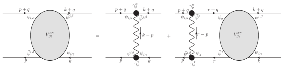
Figure 14: A diagrammatic depiction of the integral equation obeyed by offshell four point scattering amplitudes in the fermionic theory. The blob here represents the all orders scattering amplitude.

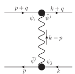
Figure 15: Fermionic tree level diagram

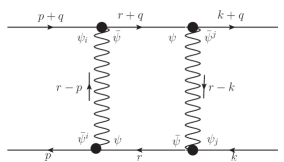
Figure 16: Fermionic 1 loop diagram

In this section we compute the four point scattering amplitude in the theory of fundamental fermions coupled to Chern-Simons theory. As in the bosonic theory, we integrate out the gauge boson to obtain an offshell effective four fermi term in the quantum effective action for our theory, given by

$$\frac{1}{2}\int\frac{d^{3}p}{(2\pi)^{3}}\frac{d^{3}k}{(2\pi)^{3}}\frac{d^{3}q}{(2\pi)^{3}}V^{\alpha\gamma}_{\beta\delta}(p,k,q){\psi}_{i,\alpha}(p+q){\bar{\psi}}^{j,\beta}(-(k+q)){\bar{\psi}}^{i,\delta}(-p)\psi_{j,\gamma}(k).$$ (134)

We then take an appropriate onshell limit to evaluate the S-matrix.

6.1 The offshell four point amplitude

As in the case of the bosonic theory, the offshell four point amplitude $V^{\alpha\gamma}_{\beta\delta}(p,k,q)$ obeys a closed Schwinger-Dyson equation. As for the bosonic theory, we work with the special case $q^{\pm}=0$. As above we first set up this Schwinger-Dyson equation for the Lorentzian theory, but find it more convenient, technically, to work with the Euclidean rotated amplitude. The Euclidean rotated amplitude is defined in a manner very similar to the bosonic theory (see below for a few more details), and may be shown to obey the Schwinger-Dyson equation

$$\begin{split}V^{\alpha\gamma}_{\beta\delta}(p,k,q)&=\frac{1}{2}(\gamma^{\mu})^{\alpha}_{\beta}G_{\mu\nu}(p-k)(\gamma^{\nu})^{\gamma}_{\delta}\\ &+\frac{1}{2}\int\frac{d^{3}r}{(2\pi^{3})}[\gamma^{\mu}G(r+q)]^{\alpha}_{\sigma}V^{\sigma\gamma}_{\beta\tau}(r,k,q)[G(r)\gamma^{\nu}]^{\tau}_{\delta}G_{\mu\nu}(p-r).\end{split}$$ (135)

Here $G(p)_{\alpha\sigma}$ is the exact fermionic propagators determined in (9) (see also [1]), while $G_{\mu\nu}$ is the gauge boson propagator defined by

$$\langle A_{\mu}^{a}(-p)A^{b}_{\nu}(q)\rangle=(2\pi)^{3}\delta^{3}(p-q)G_{\mu\nu}(q)$$ (136)

where $A_{\mu}=A^{a}T^{a}$ and we work with generators normalized so that

$$\sum_{a}(T^{a})^{i}_{j}(T^{a})^{k}_{l}=\frac{1}{2}\delta^{i}_{l}\delta^{k}_{j}.$$ (137)

And here $\gamma^{\mu}$ compose the Euclidean Clifford algebra,

$$\{\gamma^{\mu},\gamma^{\nu}\}=2\delta^{\mu\nu},\quad[\gamma^{\mu},\gamma^{\nu}]=2i\epsilon^{\mu\nu\rho}\gamma_{\rho},\qquad(\epsilon^{103}=\epsilon_{103}=1).$$

In the lightcone gauge in which we work the only nonzero components of $G_{\mu\nu}$ are

$$G_{+3}(p)=-G_{3+}(p)=\frac{4\pi~{}i}{\kappa~{}p^{+}}.$$ (138)

Now noting the fact that only non zero component is $G_{+3}(p)=-G_{3+}(p)$ and using rearrangement with $\gamma^{+}=\frac{i\gamma^{0}+\gamma^{1}}{\sqrt{2}}$,

$$(\gamma^{+})^{\alpha}_{\beta}(\gamma^{3})_{\delta}^{\gamma}-(\gamma^{3})^{\alpha}_{\beta}(\gamma^{+})_{\delta}^{\gamma}=-\left(\delta^{\gamma}_{\beta}(\gamma^{+})^{\alpha}_{\delta}-(\gamma^{+})^{\gamma}_{\beta}\delta^{\alpha}_{\delta}\right),$$ (139)

as well as

$$\gamma^{+}X\gamma^{3}-\gamma^{3}X\gamma^{+}=-2(X_{I}\gamma^{+}-X_{-}I),$$ (140)

(here $X=X_{i}\gamma^{i}+X_{I}I$ is an arbitrary $2\rightarrow 2$ matrix), we conclude that in the $\alpha,\delta$ indices of R.H.S of the Eq.(135) - and therefore the LHS , and so $V$ takes the form

$$V^{\alpha\gamma}_{\beta\delta}(p,k,q)=g(p,k,q)\delta^{\alpha}_{\delta}\delta^{\gamma}_{\beta}+f(p,k,q)(\gamma^{+})^{\alpha}_{\delta}\delta^{\gamma}_{\beta}+g_{1}(p,k,q)\delta^{\alpha}_{\delta}(\gamma^{+})^{\gamma}_{\beta}+f_{1}(p,k,q)(\gamma^{+})^{\alpha}_{\delta}(\gamma^{+})^{\gamma}_{\beta}.$$ (141)

Plugging this form $V$ into (135) yields a set of four integral equations for the four component functions in (141). We have succeeded in finding the exact solution to these equations. We present the derivation of our solution in Appendix F. The final result for this offshell amplitude is extremely complicated. The result, which takes multiple pages to write, is given in (300), (307) and (308) of the Appendix. We see no benefit in reproducing this extremely complicated final result in the main text.

6.2 The onshell limit

As we have seen above, the offshell four point function defined in (134) is quite a complicated object. In this section we will argue that the onshell S-matrix is, however, rather simple.

In order to study the S-matrix it is first convenient to continue our result for $V$ in (134) to Minkowski space. This is achieved by making the substitution

$$p^{0}\rightarrow-ip^{0},~{}~{}~{}k^{0}\rightarrow-ik^{0},~{}~{}~{}\gamma^{0}\rightarrow-i\gamma^{0},$$

on the Euclidean result of the previous subsection. This substitution yields the four fermi term in the effective action (85) in Lorentzian space.

In order to convert this four point vertex to a scattering amplitude, we must now go onshell. We now pause to carefully explain how this is achieved.

In free field theory (i.e. in the absence of the four point function interaction) the fermion field operators may be expanded in creation and annihilation modes in the standard fashion

$$\begin{split}\psi(x)&=\int\frac{d^{3}p}{(2\pi)^{3}}\psi(p)e^{ip\cdot x}\\ &=\int\frac{d^{2}p}{(2\pi)^{2}}\frac{1}{\sqrt{2~{}E_{p}}}\left(u(\vec{p})a_{\vec{p}}e^{ip\cdot x}+v(\vec{p})b_{\vec{p}}^{\dagger}e^{-ip\cdot x}\right),\\ {\bar{\psi}}(x)&=\int\frac{d^{3}p}{(2\pi)^{3}}{\bar{\psi}}(p)e^{ip\cdot x}\\ &=\int\frac{d^{2}p}{(2\pi)^{2}}\frac{1}{\sqrt{2~{}E_{p}}}\left({\bar{u}}(\vec{p})a_{\vec{p}}^{\dagger}e^{-ip\cdot x}+{\bar{v}}(\vec{p})b_{\vec{p}}e^{ip\cdot x}\right),\end{split}$$ (142)

where $p^{0}=\omega=\sqrt{c_{F}^{2}+p_{1}^{2}+p_{3}^{2}}$. As always we use the mostly positive convention, so $e^{ip.x}$ has negative ‘frequency’ in time, while $e^{-ip.x}$ has positive frequency in time. As is usual, the coefficients of negative frequency wave functions are annihilation operators, while the coefficients of positive frequency wave functions are creation operators. We refer to $a$ and $a^{\dagger}$ as particle destruction and creation operators, while $b$ and $b^{\dagger}$ are antiparticle destruction and creation operators. The wave functions $u(p)e^{ip.x}$ and $v(p)e^{-ip.x}$ are solutions to the Dirac equation

$$\left(i(p_{\mu}+\Sigma_{\mu})\gamma^{\mu}+\Sigma_{I}\right)\psi(p)=0$$

and, as usual, ${\bar{\psi}}=i\psi^{\dagger}\gamma^{0}$, where $\Sigma$ is defined in (10). For later convenience, we introduce the following notation,

$$\Sigma_{I}(p_{s})=f(p_{s})p_{s},~{}~{}~{}\Sigma_{+}=g(p_{s})p_{s}.$$

The Dirac equation uniquely determines $u(p)$ and $v(p)$ upto multiplicative constants. We fix the normalization ambiguity by demanding

$$\bar{u}(\vec{p})u(\vec{p})=2f(p_{s})p_{s},~{}~{}~{}\bar{v}(\vec{p})v(\vec{p})=-2f(p_{s})p_{s}.$$ (143)

These requirements leave the phase of the functions $u(p)$ and $v(p)$ undetermined: we will make an arbitrary choice for this phase below.

We will find it useful to have explicit expressions for $u$ and $v$. In order to obtain these expressions, it is useful to fix a particular convention for $\gamma$ matrices. In Euclidean space we make the choice $\gamma^{+}=\left(\begin{array}[]{cc}0&\sqrt{2}\\ 0&0\end{array}\right)$, $\gamma^{-}=\left(\begin{array}[]{cc}0&0\\ \sqrt{2}&0\end{array}\right)$ and $\gamma^{3}=\left(\begin{array}[]{cc}1&0\\ 0&-1\end{array}\right).$ This choice determines the Lorentzian $\gamma$ matrices to be

$$\begin{split}\gamma^{3}=\left(\begin{array}[]{cc}1&0\\ 0&-1\end{array}\right),\qquad\gamma^{+}=\left(\begin{array}[]{cc}0&\sqrt{2}\\ 0&0\end{array}\right),\\ \gamma^{-}=\left(\begin{array}[]{cc}0&0\\ \sqrt{2}&0\end{array}\right),\qquad\gamma^{0}=\left(\begin{array}[]{cc}0&1\\ -1&0\end{array}\right).\end{split}$$ (144)

The quadratic Dirac Lagrangian consequently takes the explicit form

$$\int\frac{d^{3}p}{(2\pi)^{3}}\bar{\psi}(-p)\left(\begin{array}[]{cc}ip_{2}+f(p_{s})p_{s}&i\sqrt{2}p_{+}(1+g(p_{s}))\\ i\sqrt{2}p_{-}&-ip_{2}+f(p_{s})p_{s}\end{array}\right)\psi(p).$$ (145)

The equations of motion for $u$ and ${\bar{u}}$ are

$$\begin{split}\left(\begin{array}[]{cc}ip_{2}+f(p_{s})p_{s}&-i(E_{\vec{p}}-p_{1})(1+g(p_{s}))\\ i(E_{\vec{p}}+p_{1})&-ip_{2}+f(p_{s})p_{s}\end{array}\right)u(\vec{p})&=0,\\ \bar{u}(\vec{p})\left(\begin{array}[]{cc}ip_{2}+f(p_{s})p_{s}&-i(E_{\vec{p}}-p_{1})(1+g(p_{s}))\\ i(E_{\vec{p}}+p_{1})&-ip_{2}+f(p_{s})p_{s}\end{array}\right)&=0,\end{split}$$ (146)

while those for $v$ and ${\bar{v}}$ are

$$\begin{split}\left(\begin{array}[]{cc}ip_{2}-f(p_{s})p_{s}&-i(E_{\vec{p}}-p_{1})(1+g(p_{s}))\\ i(E_{\vec{p}}+p_{1})&-ip_{2}-f(p_{s})p_{s}\end{array}\right)v(\vec{p})&=0,\\ \bar{v}(\vec{p})\left(\begin{array}[]{cc}ip_{2}-f(p_{s})p_{s}&-i(E_{\vec{p}}-p_{1})(1+g(p_{s}))\\ i(E_{\vec{p}}+p_{1})&-ip_{2}-f(p_{s})p_{s}\end{array}\right)&=0.\end{split}$$ (147)

Note that, (146) and (147) admits solution only when, determinant of the matrix appearing in those equations are zero. This gives onshell condition $p^{2}+c_{F}^{2}=0,$ equivalently

$$p_{2}^{2}+f(p_{s})^{2}p_{s}^{2}-\left(E_{\vec{p}}^{2}-p_{1}^{2}\right)\left(1+g(p_{s})\right)=0.$$

Solving these equations subject to the normalization conventions described above (plus an arbitrary choice of phase) we find

$$\begin{split}u(\vec{p})&=\frac{1}{\sqrt{E_{\vec{p}}+p_{1}}}\begin{pmatrix}ip_{2}-f(p_{s})p_{s}\\ i(E_{\vec{p}}+p_{1})\end{pmatrix},\\ \bar{u}(\vec{p})&=\frac{1}{\sqrt{E_{\vec{p}}+p_{1}}}\left(\begin{array}[]{cc}-(E_{\vec{p}}+p_{1})&~{}~{}~{}p_{2}-if(p_{s})p_{s}\end{array}\right),\end{split}$$ (148)

and

$$\begin{split}v(\vec{p})&=\frac{1}{\sqrt{E_{\vec{p}}+p_{1}}}\left(\begin{array}[]{c}ip_{2}+f(p_{s})p_{s}\\ i(E_{\vec{p}}+p_{1})\end{array}\right),\\ \bar{v}(\vec{p})&=\frac{1}{\sqrt{E_{\vec{p}}+p_{1}}}\left(\begin{array}[]{cc}-(E_{\vec{p}}+p_{1})&~{}~{}~{}p_{2}+if(p_{s})p_{s}\end{array}\right).\end{split}$$ (149)

6.3 S-matrices

With explicit expressions for $u({\vec{p}})$ and $v({\vec{p}})$ in hand, it might seem like an easy task to take the onshell limit of the ofshell 4 Fermi correlators. Infact that is not the case. As in the bosonic theory the onshell limit of these correlators is apparently ambiguous, and must be taken very carefully. The reader will recall that we discussed this issue at great detail in the bosonic theory, came to the conclusion that the correct final prescription is simply to first set $|{\vec{k}}|$ to $|{\vec{p}}|$ before taking either of these momenta individuallyonshell. We adopt a similar prescription for the bosonic theories. We first replace the quantities $E_{p}$ and $E_{k}$ that appear in our solutions for $u({\vec{p}})$ and $v({\vec{p}})$ with $\pm p^{0}$ and $\pm k^{0}$ respectively. We then evaluate the offshell amplitude with $|{\vec{k}}|=|{\vec{p}}|$ and only then take the momenta to individually be onshell. This process yields unambiguous answers which we present below. As in the bosonic case, it should be possible to justify this order of limits with a careful evaluation of the amplitude directly in Minkoski space keeping careful track of the factors of $i\epsilon$ but we have not persued this thought.

6.3.1 S-matrix for adjoint exchange in particle - antiparticle scattering

As we have explained above, the offshell four fermion scattering amplitude is extremely complicated. Quite remarkably, however, the onshell limit displays remarkable simplifications. In the $T$-channel the onshell S-matrix is given by

$$\begin{split}T_{T}^{F}&=V^{\alpha\gamma}_{\beta\delta}(p,k,q){u}_{i,\alpha}(p+q){\bar{v}}^{j,\beta}(-(k+q)){\bar{u}}^{i,\delta}(p)v_{j,\gamma}(-k)\\ &=-\frac{4\pi i}{k_{F}}q_{3}\frac{p_{-}+k_{-}}{p_{-}-k_{-}}\\ &-\frac{4i\pi}{k_{F}}q_{3}~{}~{}\frac{\left(q_{3}-2i~{}{\rm sgn}(m_{F})|c_{F}|\right)e^{2i\lambda_{F}\tan^{-1}\left(\frac{2|c_{F}|}{q_{3}}\right)}-e^{i\pi{\rm sgn}(q_{3})\lambda_{F}}\left(q_{3}+2i~{}{\rm sgn}(m_{F})|c_{F}|\right)}{e^{i\pi{\rm sgn}(q_{3})\lambda_{F}}\left(q_{3}+2i~{}{\rm sgn}(m_{F})|c_{F}|\right)+\left(q_{3}-2i~{}{\rm sgn}(m_{F})|c_{F}|\right)e^{2i\lambda_{F}\tan^{-1}\left(\frac{2|c_{F}|}{q_{3}}\right)}}\\ &=-E(p_{1},p_{2},p_{3})\frac{4i\pi}{k_{F}}\sqrt{\frac{u~{}t}{s}}\\ &-\frac{4i\pi}{k_{F}}\sqrt{-t}~{}~{}\frac{\left(\sqrt{-t}-2i~{}{\rm sgn}(m_{F})|c_{F}|\right)e^{2i\lambda_{F}\tan^{-1}\left(\frac{2|c_{F}|}{\sqrt{-t}}\right)}-e^{i\pi\lambda_{F}}\left(\sqrt{-t}+2i~{}{\rm sgn}(m_{F})|c_{F}|\right)}{e^{i\pi\lambda_{F}}\left(\sqrt{-t}+2i~{}{\rm sgn}(m_{F})|c_{F}|\right)+\left(\sqrt{-t}-2i~{}{\rm sgn}(m_{F})|c_{F}|\right)e^{2i\lambda_{F}\tan^{-1}\left(\frac{2|c_{F}|}{\sqrt{-t}}\right)}}\\ &=-E(p_{1},p_{2},p_{3})\frac{4i\pi}{k_{F}}\sqrt{\frac{u~{}t}{s}}\\ &-\frac{4i\pi}{k_{F}}\sqrt{-t}~{}~{}\frac{\left(\sqrt{-t}-2i~{}{\rm sgn}(m_{F})|c_{F}|\right)e^{2i\lambda_{F}\tan^{-1}\left(\frac{2|c_{F}|}{\sqrt{-t}}\right)}-e^{i\pi\lambda_{F}}\left(\sqrt{-t}+2i~{}{\rm sgn}(m_{F})|c_{F}|\right)}{e^{i\pi\lambda_{F}}\left(\sqrt{-t}+2i~{}{\rm sgn}(m_{F})|c_{F}|\right)+\left(\sqrt{-t}-2i~{}{\rm sgn}(m_{F})|c_{F}|\right)e^{2i\lambda_{F}\tan^{-1}\left(\frac{2|c_{F}|}{\sqrt{-t}}\right)}}\\ &=-E(p_{1},p_{2},p_{3})\frac{4i\pi}{k_{F}}\sqrt{\frac{u~{}t}{s}}+\frac{4~{}i\pi}{k_{F}}\sqrt{-t}~{}~{}\frac{e^{i\pi\left(\lambda_{F}-{\rm sgn}(m_{F})\right)}+e^{2i\left(\lambda_{F}-{\rm sgn}(m_{F})\right)\tan^{-1}\left(\frac{2|c_{F}|}{\sqrt{-t}}\right)}}{e^{i\pi\left(\lambda_{F}-{\rm sgn}(m_{F})\right)}-e^{2i\left(\lambda_{F}-{\rm sgn}(m_{F})\right)\tan^{-1}\left(\frac{2|c_{F}|}{\sqrt{-t}}\right)}}~{}~{}\\ &=-E(p_{1},p_{2},p_{3})\frac{4i\pi}{k_{F}}\sqrt{\frac{u~{}t}{s}}+\frac{4~{}i\pi}{k_{F}}\sqrt{-t}~{}~{}\frac{1+e^{-2i\left(\lambda_{F}-{\rm sgn}(m_{F})\right)\tan^{-1}\left(\frac{\sqrt{-t}}{2|c_{F}|}\right)}}{1-e^{-2i\left(\lambda_{F}-{\rm sgn}(m_{F})\right)\tan^{-1}\left(\frac{\sqrt{-t}}{2|c_{F}|}\right)}}.~{}~{}\\ \end{split}$$ (150)

As we have emphasized above, we have obtained this result only after taking the onshell limit in a particular manner. In particular, in the solution in (148),(149) we treated $E_{p}$ as a free symbol to start with; we set $p_{s}=k_{s}$ first and then set $E_{p}^{2}={\overrightarrow{p}}^{2}+c_{F}^{2}.$

6.3.2 S-matrix for particle - particle scattering

In the $U$-channel

$$\begin{split}T_{U_{d}}^{F}&=V^{\alpha\gamma}_{\beta\delta}(p,k,q){u}_{i,\alpha}(p+q){\bar{u}}^{j,\beta}(k+q){\bar{u}}^{i,\delta}(p)u_{j,\gamma}(k)\\ &=\frac{4\pi i}{k_{F}}q_{3}\frac{p_{-}+k_{-}}{p_{-}-k_{-}}\\ &+\frac{4i\pi}{k_{F}}q_{3}~{}~{}\frac{\left(q_{3}-2i~{}{\rm sgn}(m_{F})|c_{F}|\right)e^{2i\lambda_{F}\tan^{-1}\left(\frac{2|c_{F}|}{q_{3}}\right)}-e^{i\pi{\rm sgn}(q_{3})\lambda_{F}}\left(q_{3}+2i~{}{\rm sgn}(m_{F})|c_{F}|\right)}{e^{i\pi{\rm sgn}(q_{3})\lambda_{F}}\left(q_{3}+2i~{}{\rm sgn}(m_{F})|c_{F}|\right)+\left(q_{3}-2i~{}{\rm sgn}(m_{F})|c_{F}|\right)e^{2i\lambda_{F}\tan^{-1}\left(\frac{2|c_{F}|}{q_{3}}\right)}}\\ &=-\Bigg{(}E(p_{1},p_{2},p_{3})\frac{4i\pi}{k_{B}}\sqrt{\frac{s~{}t}{u}}\\ &-\frac{4i\pi}{k_{F}}\sqrt{-t}~{}~{}\frac{\left(\sqrt{-t}-2i~{}{\rm sgn}(m_{F})|c_{F}|\right)e^{2i\lambda_{F}\tan^{-1}\left(\frac{2|c_{F}|}{\sqrt{-t}}\right)}-e^{i\pi\lambda_{F}}\left(\sqrt{-t}+2i~{}{\rm sgn}(m_{F})|c_{F}|\right)}{e^{i\pi\lambda_{F}}\left(\sqrt{-t}+2i~{}{\rm sgn}(m_{F})|c_{F}|\right)+\left(\sqrt{-t}-2i~{}{\rm sgn}(m_{F})|c_{F}|\right)e^{2i\lambda_{F}\tan^{-1}\left(\frac{2|c_{F}|}{\sqrt{-t}}\right)}}\Bigg{)}\\ &=-\Bigg{(}-E(p_{1},p_{2},p_{3})\frac{4i\pi}{k_{F}}\sqrt{\frac{s~{}t}{u}}+\frac{4~{}i\pi}{k_{F}}\sqrt{-t}~{}~{}\frac{e^{i\pi\left(\lambda_{F}-{\rm sgn}(m_{F})\right)}+e^{2i\left(\lambda_{F}-{\rm sgn}(m_{F})\right)\tan^{-1}\left(\frac{2|c_{F}|}{\sqrt{-t}}\right)}}{e^{i\pi\left(\lambda_{F}-{\rm sgn}(m_{F})\right)}-e^{2i\left(\lambda_{F}-{\rm sgn}(m_{F})\right)\tan^{-1}\left(\frac{2|c_{F}|}{\sqrt{-t}}\right)}}~{}~{}\Bigg{)}\\ &=-\Bigg{(}-E(p_{1},p_{2},p_{3})\frac{4i\pi}{k_{F}}\sqrt{\frac{s~{}t}{u}}+\frac{4~{}i\pi}{k_{F}}\sqrt{-t}~{}~{}\frac{1+e^{-2i\left(\lambda_{F}-{\rm sgn}(m_{F})\right)\tan^{-1}\left(\frac{\sqrt{-t}}{2|c_{F}|}\right)}}{1-e^{-2i\left(\lambda_{F}-{\rm sgn}(m_{F})\right)\tan^{-1}\left(\frac{\sqrt{-t}}{2|c_{F}|}\right)}}~{}~{}\Bigg{)}.\\ \end{split}$$ (151)

As in the previous subsubsection, we have obtained this resultafter taking the onshell limit in a particular manner. In particular, in the solution in (148),(149) we treated $E_{p}$ as a free symbol to start with; we set $p_{s}=k_{s}$ first and then set $E_{p}^{2}={\overrightarrow{p}}^{2}+c_{F}^{2}.$

7 Scattering in the identity channel and crossing symmetry

7.1 Crossing symmetry

It is sometimes asserted that the S-matrix for particle - antiparticle scattering, in any quantum field theory, may be obtained from the S-matrix for particle - particle scattering. This claim goes by the name of crossing symmetry. In the context of the $2\rightarrow 2$ scattering studied in this paper, the formulae asserted with the claim are (we work with the bosonic theory for definiteness)

$$T_{S}(s,t,u)=NT_{U_{d}}(t,u,s),~{}~{}~{}~{}T_{T}(s,t,u)=T_{U_{d}}(u,t,s).$$ (152)

These equations assert that the formulae for particle - antiparticle scattering may be read off from the analytic continuation of the physical particle - particle scattering amplitude .

In the case of an ungauged field theory - or in the case of the scattering of gauge invariant particles in a gauge theory, there is a rather straightforward intuitive argument for crossing symmetry of amplitudes. The LSZ formula relates S-matrices to onshell limits of well-defined offshell correlators. The offshell correlators are expected to be analytic functions of their insertion positions. The on shell limit of these correlators is the ‘master function’ referred to in the footnote above which plausibly inherits analytic properties from those of the underlying correlators.

This intuitive argument does not work for the scattering of non gauge singlet particles in a gauge theory, as the relevant scattering amplitudes cannot be obtained from the onshell limit of an offshell correlator (the putative offshell correlators are not gauge invariant and so are ill defined).

While the argument for crossing symmetry presented in this subsection does not apply to, for instance, the scattering of gluons in ${\cal N}=4$ Yang Mills theory, the final result (i.e. that scattering amplitudes obey crossing symmetry) is widely expected to hold true for these amlitudes, at least with a suitable definition of the scattering amplitudes (a definition is needed to deal with IR ambiguities having to do with soft gluons and other soft particles). In this context we expect that the failure of the argument outlined in this subsection is just a technicality; other arguments (perhaps based on diagrammatics) guarantee the final result.

As in the previous paragraph, current paper we are also interested in the scattering of non singlet excitations. Unlike the case of gluonic scattering in ${\cal N}=4$ Yang Mills, however, we will argue below that the failure of the argument for crossing symmetry is more than a technicality. The crossing relations are actually modified in our theories. We suspect that the underlying reason for the modification is that the Chern-Simons action, which controls the dynamics of our gauge fields, effectively turns our scattering particles into anyons. Apparently, the usual crossing relations are true for the scattering of bosons and fermions, but are modified in the scattering of anyons.

7.2 A conjecture for the S-matrix in the singlet channel

As we have explained above, a naive application of crossing symmetry predicts that, the $S$-channel scattering amplitude is given by $T_{S}^{B}(s,t,u)=NT^{B}_{U_{d}}(t,u,s)$. We have performed the analytic continuations needed to make sense of this formula in subsection 4.4. Utilizing the results of that subsection, the naive prediction of crossing symmetry is

$$\begin{split}&T_{S}^{trial}=\left(\pi\lambda_{B}\right)4i\sqrt{s}E(p_{1},p_{2},p_{3})\sqrt{\frac{u}{t}}+j^{M}(\sqrt{s})\\ &=\left(\pi\lambda_{B}\right)4\sqrt{s}\left(i~{}E(p_{1},p_{2},p_{3})\sqrt{\frac{u}{t}}+\left(\frac{\left(4\pi\lambda_{B}\sqrt{s}+\widetilde{b}_{4}\right)+\left(-4\pi\lambda_{B}\sqrt{s}+\widetilde{b}_{4}\right)e^{8\pi\lambda_{B}\sqrt{s}H^{M}(\sqrt{s})}}{\left(4\pi\lambda_{B}\sqrt{s}+\widetilde{b}_{4}\right)-\left(-4\pi\lambda_{B}\sqrt{s}+\widetilde{b}_{4}\right)e^{8\pi\lambda_{B}\sqrt{s}H^{M}(\sqrt{s})}}\right)\right)\\ &=\left(\pi\lambda_{B}\right)4\sqrt{s}\left(i~{}E(p_{1},p_{2},p_{3})\sqrt{\frac{u}{t}}+\left(\frac{\left(4\pi\lambda_{B}\sqrt{s}+\widetilde{b}_{4}\right)+e^{i\pi\lambda_{B}}\left(-4\pi\lambda_{B}\sqrt{s}+\widetilde{b}_{4}\right)\left(\frac{\frac{1}{2}+\frac{c_{B}}{\sqrt{s}}}{\frac{1}{2}-\frac{c_{B}}{\sqrt{s}}}\right)^{\lambda_{B}}}{\left(4\pi\lambda_{B}\sqrt{s}+\widetilde{b}_{4}\right)-e^{i\pi\lambda_{B}}\left(-4\pi\lambda_{B}\sqrt{s}+\widetilde{b}_{4}\right)\left(\frac{\frac{1}{2}+\frac{c_{B}}{\sqrt{s}}}{\frac{1}{2}-\frac{c_{B}}{\sqrt{s}}}\right)^{\lambda_{B}}}\right)\right)\\ \end{split}$$ (153)

(in the last line we have specialized to the physical domain $s\geq 4c_{B}^{2}$).

The function $T_{S}^{trial}$ cannot be the true scattering matrix in the $S$-channel for three related reasons.

• $T_{S}^{trial}$ does not include the last term in (53); a term delta function localized on forward scattering with a coefficient proportional to $(\cos(\pi\lambda_{B})-1)$. This term is certainly present in the scattering amplitude at least in the non-relativistic limit.

• Even ignoring the term localized at forward scattering, the non-relativistic limit of $T_{S}^{trial}$ does not agree with (53).

• $T_{S}^{trial}$ does not obey the unitarity relation (64).

In the rest of this subsection we will demonstrate that all these problems are simultaneously cured if we conjecture that the scattering matrix in the $S$-channel is given by a rescaled $T_{S}^{trial}$ plus a contact term added by hand. We conjecture that the bosonic scattering matrix in the $S$-channel is given by

$$T_{S}^{B}=\frac{\sin(\pi\lambda_{B})}{\pi\lambda_{B}}T_{S}^{trial}-i(\cos(\pi\lambda_{B})-1)I(p_{1},p_{2},p_{3},p_{4})$$ (154)

(see subsection 2.3 for a definition of the Identity matrix). In subsection 7.4 we will present a tentative justification for the modification of the usual rules of crossing symmetry implicit in (81). In the rest of this subsection we will demonstrate that the conjectured scattering amplitude $T_{S}^{B}$ passes various consistency checks.

In the center of mass frame our conjectured scattering amplitude (154) takes the form (65) with

$$\begin{split}&H(\sqrt{s})=4\sqrt{s}\sin(\pi\lambda_{B}),\\ &W_{1}(\sqrt{s})=4\sqrt{s}\sin(\pi\lambda_{B})G,\\ &W_{2}(\sqrt{s})=8\pi\sqrt{s}\left(\cos(\pi\lambda_{B})-1\right),\\ &G=\left(\frac{\left(4\pi\lambda_{B}\sqrt{s}+\widetilde{b}_{4}\right)+e^{i\pi{\lambda_{B}}}\left(-4\pi{\lambda_{B}}\sqrt{s}+\widetilde{b}_{4}\right)\left(\frac{\frac{1}{2}+\frac{c_{B}}{\sqrt{s}}}{\frac{1}{2}-\frac{c_{B}}{\sqrt{s}}}\right)^{\lambda_{B}}}{\left(4\pi{\lambda_{B}}\sqrt{s}+\widetilde{b}_{4}\right)-e^{i\pi{\lambda_{B}}}\left(-4\pi{\lambda_{B}}\sqrt{s}+\widetilde{b}_{4}\right)\left(\frac{\frac{1}{2}+\frac{c_{B}}{\sqrt{s}}}{\frac{1}{2}-\frac{c_{B}}{\sqrt{s}}}\right)^{\lambda_{B}}}\right).\end{split}$$ (155)

Let us first demonstrate that our conjectured expressions (155) have the correct non-relativistic limit. The functions $H$ and $W_{2}$ in (66) are independent of the energy $s$ and already agree perfectly with the same functions in (66). Moreover

$$\lim_{\sqrt{s}\rightarrow 2c_{B}}G=-{\rm sgn}({\lambda_{B}})$$ (156)

it follows that

$$\lim_{\sqrt{s}\to 2c_{B}}W_{1}(\sqrt{s})=-4\sqrt{s}|\sin(\pi{\lambda_{B}})|$$ (157)

in agreement with (66). We conclude that our conjectured scattering amplitude (155) reduces precisely to the expected Aharonov-Bohm scattering amplitude in the non-relativistic limit.

We next demonstrate that our conjecture for the $S$-channel S-matrix obeys the constraints of unitarity, i.e. that (155) obeys the equations (70). As we have explained in subsection 2.7.4, the fact that $H$ and $W_{2}$ in (155) agree with the corresponding functions in (66) immediately implies that the first two equations in (70) are obeyed. We will now demonstrate that the functions in (155) also obey the third equation in (70).

The third equation in (70) may be rewritten, in terms of the function $G$, as

$$G-G^{*}=(1-\cos(\pi{\lambda_{B}}))(G-G^{*})-i\sin(\pi{\lambda_{B}})(1-GG^{*})$$

This equation is holds if

$$G-G^{*}=-i\tan(\pi{\lambda_{B}})(1-GG^{*}).$$ (158)

Now

$$G=\frac{1+e^{i\pi{\lambda_{B}}}y}{1-e^{i\pi{\lambda_{B}}}y},$$

where

$$y=\frac{\left(-4\pi{\lambda_{B}}\sqrt{s}+\widetilde{b}_{4}\right)}{\left(4\pi{\lambda_{B}}\sqrt{s}+\widetilde{b}_{4}\right)}\left(\frac{\frac{1}{2}+\frac{c_{B}}{\sqrt{s}}}{\frac{1}{2}-\frac{c_{B}}{\sqrt{s}}}\right)^{\lambda_{B}}.$$

Note in particular that $y$ is real (its detailed form is irrelevant for what follows). It follows that

$$G-G^{*}=\frac{4iy\sin(\pi{\lambda_{B}})}{|1-e^{i\pi{\lambda_{B}}}y|^{2}},~{}~{}~{}(1-GG^{*})=\frac{-4y\cos(\pi{\lambda_{B}})}{|1-e^{i\pi{\lambda_{B}}}y|^{2}}.$$

It follows that (158) is satisfied so that our proposal (81) defines a unitary S-matrix.

Finally, in the limit ${\lambda_{B}}\to 0$, our conjecture reduces to (see the second line of (82))

$$T_{S}^{B}=\frac{-b_{4}}{1+b_{4}H^{M}(\sqrt{s})}.$$

It is easily independently verified that this is the correct formula for the scattering amplitude of the large $N$ $\phi^{4}$ theory that (5) reduces to in the small ${\lambda_{B}}$ limit. In other words our conjectured scattering amplitude has the correct small ${\lambda_{B}}$ limit.

7.3 Bose-Fermi duality in the $S$-channel

We have conjectured above that, in the $S$-channel, the bosonic S-matrix is given by

$$T_{S}^{B}(s,t,u,\lambda_{B})=\frac{k_{B}\sin(\pi\lambda_{B})}{\pi}T_{U_{d}}^{B}(t,u,s,\lambda_{B})-i\left(\cos(\pi\lambda_{B})-1\right)I(p_{1},p_{2},p_{3},p_{4}),$$ (159)

This implies that the S-matrix in the $S$-channel is given by

$$S_{S}^{B}(s,t,u,\lambda_{B})=i\frac{k_{B}\sin(\pi\lambda_{B})}{\pi}T_{U_{d}}^{B}(t,u,s,\lambda_{B})+\cos(\pi\lambda_{B})I(p_{1},p_{2},p_{3},p_{4}),$$ (160)

where $I$ is the identity S-matrix, see subsection 2.3.

In this section we have, so far, presented our conjecture for the $S$-channel S-matrix in the bosonic theory. It is natural to conjecture a similar formula in the fermionic theory. In analogy with our conjecture for the bosonic theory we conjecture that

$$T_{S}^{F}(s,t,u,\lambda_{F})=\frac{k_{F}\sin(\pi\lambda_{F})}{\pi}T_{U_{d}}^{F}(t,u,s,\lambda_{F})-i\left(\cos(\pi\lambda_{F})-1\right)I(p_{1},p_{2},p_{3},p_{4})$$ (161)

so that

$$S_{S}^{F}(s,t,u,\lambda_{F})=i\frac{k_{F}\sin(\pi\lambda_{F})}{\pi}T_{U_{d}}^{F}(t,u,s,\lambda_{F})+\cos(\pi\lambda_{F})I(p_{1},p_{2},p_{3},p_{4}).$$ (162)

We will now demonstrate that these two conjectures map to each other under duality.

$$\begin{split}&\frac{k_{B}\sin(\pi\lambda_{B})}{\pi}=\frac{k_{F}\sin(\pi\lambda_{F})}{\pi},\\ &T_{U_{d}}^{B}(t,u,s,\lambda_{B})=-T_{U_{d}}^{F}(t,u,s,\lambda_{F}),\\ &\cos(\pi\lambda_{B})=-\cos(\pi\lambda_{F}),\\ \end{split}$$ (163)

(through this subsection we specialize to the limit $b_{4}\to\infty$ in the bosonic theory). it follows that

$$S_{S}^{B}(s,t,u,\lambda_{B})=-S_{S}^{F}(s,t,u,\lambda_{F}),$$ (164)

which implies that

$$\begin{split}S_{S}^{F}(s,t,u,\lambda_{F})=&\sin(\pi\lambda_{F})\Bigg{(}4E(p_{1},p_{2},p_{3})\sqrt{\frac{s~{}t}{u}}+4\sqrt{s}~{}~{}\frac{1+e^{-2i\left(\lambda_{F}-{\rm sgn}(m_{F})\right)\tan^{-1}\left(\frac{\sqrt{s}}{2|c_{F}|}\right)}}{1-e^{-2i\left(\lambda_{F}-{\rm sgn}(m_{F})\right)\tan^{-1}\left(\frac{\sqrt{s}}{2|c_{F}|}\right)}}~{}~{}\Bigg{)}\\ &+\cos(\pi\lambda_{F})I(p_{1},p_{2},p_{3},p_{4}).\end{split}$$ (165)

Note that, $S_{S}^{F}(s,t,u,\lambda_{F})$ reduces to correct tree level S-matrix presented in section 2.5. The overall minus sign on the RHS of (164) has no physical significance, as the sign of fermionic scattering amplitudes is largely a matter of convention. (164) demonstrates the unitarity singlet fermionic S-matrix obtained from the conjecture (162), as we have already checked the unitarity of the bosonic S-matrix.

In summary, our conjecture for the $S$-channel S-matrices is consistent with Bose-Fermi duality. This observation may be taken as one more piece of evidence in support of our conjecture.

7.4 A heuristic explanation for modified crossing symmetry

In this section we have conjectured that the naive crossing symmetry (152) are modified in fundamental matter Chern-Simons theory; in the large N limit of interest to this paper, we have proposed that the second of (152) continues to apply, while the first of (152) is replaced by (81). The arguments presented so far for this replacement have been entirely pragmatic; we guessed the modified crossing relation in order that the S-matrix in the $S$-channel obey various consistency conditions.

In this subsection we will attempt to sketch a logical explanation for this modified crossing relation (82). Our explanation is heuristic in several respects, but we hope that its defects will be remedied by more careful studies in the future.

The starting point of our analysis is the argument for crossing symmetry in the bosonic theory in the limit ${\lambda_{B}}\to 0$, briefly alluded to in subsection 7.1. When ${\lambda_{B}}$ is set to zero, the bosonic theory effectively reduces to a theory of scalars with global $U(N)$ symmetry . In this theory the offshell correlator

$$C=\langle\phi_{i}(x_{1}){\bar{\phi}}^{j}(x_{2}){\bar{\phi}}^{k}(x_{3})\phi_{m}(x_{4})\rangle$$ (166)

is a well-defined meromorphic function of its arguments. By $U(N)$ invariance this correlator is given by

$$C_{im}^{jk}(x_{1},x_{2},x_{3},x_{4})=A(x_{1},x_{2},x_{3},x_{4})\delta_{i}^{j}\delta_{m}^{k}+B(x_{1},x_{2},x_{3},x_{4})\delta_{i}^{k}\delta_{m}^{j}$$ (167)

where the coefficient functions $A$ and $B$ are functions of the insertion points $x^{1}\ldots x^{4}$. crossing symmetry follows from the observation that distinct scattering amplitudes are simply distinct onshell limits of the same correlators.

This statement is usually made precise in momentum space, but we will find it more convenient to work in position space. Consider an $S^{2}$ of size $R$, inscribed around the origin in Euclidean $R^{3}$ (we will eventually be interested in the limit $R\to\infty$). The S-matrices $S_{U_{d}}$ and $S_{S}$ may both be obtained from the correlator $A$ as follows. Consider free incoming particles of momentum $p_{i}$ and $p_{m}$ starting out at very early times and focussed so that their worldlines will both intersect the origin of $R^{3}$. These two world lines intersect the $S^{2}$ described above at easily determined locations $x_{1}$ and $x_{4}$ respectively. Similarly the coordinates $x_{2}$ and $x_{3}$ are chosen to be the intercepts of the world lines of particles with index $j$ and $k$, starting out from the origin of $R^{3}$ and proceeding to the future along world lines of momentum $p_{2}$ and $p_{3}$ respectively. Having now chosen the insertion points of all operators as definite functions of momenta, the correlator $A(x_{1},x_{2},x_{3},x_{4})$ is now a function only of the relevant particle - particle scattering data; the particle-particle S-matrix may infact be read off from this correlator in the limit $R\to\infty$ after we strip off factors pertaining to free propagation of our particles from the surface of the $S^{2}$ to the origin of $R^{3}$. Particle- antiparticle scattering may be obtained in an identical manner, by choosing $x_{1}$ and $x_{2}$ to lie along the trajectory of incoming particles or antiparticles of momentum $p_{1}$ and $p_{2}$ respectively, while $x_{3}$ and $x_{4}$ lie along particle trajectories of outgoing particles and antiparticles of momentum $p_{3}$ and $p_{4}$ respectively. Intuitively we expect that crossing symmetry - the first of (152) - follows from the analyticity of the correlator $A$ as a function of $x_{1}$, $x_{2}$, $x_{3}$ and $x_{4}$ on the large $S^{2}$.

In the large $N$ limit $A$ may be obtained from the correlator $C_{im}^{jk}$ in (167) from the identity

$$A=\frac{1}{N^{2}}C^{jk}_{im}\delta_{j}^{i}\delta_{k}^{m}$$ (168)

At nonzero ${\lambda_{B}}$ the correlator $C_{im}^{jk}$ no longer makes sense as it is not gauge invariant. In order to construct an appropriate gauge invariant quantity let $W_{12}$ denote an open Wilson line, in the fundamental representation, starting at $x_{1}$, ending at $x_{2}$ and running entirely outside the $S^{2}$ one which the operators are inserted. In a similar manner let $W_{43}$ denote an open Wilson starting at $x_{4}$ and ending at $x_{3}$, once again traversing a path that lies entirely outside the $S^{2}$ on which operators are inserted. Then the quantity

$$A^{\prime}=C_{im}^{jk}(W_{12})^{i}_{j}(W_{43})^{m}_{k}$$ (169)

is a rough analogue of $A$ in the gauged theory. The precise relationship is that $A^{\prime}$ reduces to $A$ in the limit ${\lambda_{B}}\to 0$ in which gauge dynamics decouples from matter dynamics. $A^{\prime}$ is clearly gauge invariant at all ${\lambda_{B}}$; moreover there seems no reason to doubt that $A^{\prime}$ is an analytic function of $x_{1}\ldots x_{4}$.

We can now evaluate $A^{\prime}$ in the same two onshell limits discussed in the paragraph above; as in the paragraph above this yields two functions of onshell momenta that are analytic continuations of each other. In the limit ${\lambda_{B}}\to 0$ these two functions are simply the direct channel and singlet channel S-matrices. We will now address the following question: what is the interpretation of these two functions, obtained out of $A^{\prime}$, at finite ${\lambda_{B}}$?

The path integral that evaluates the quantity $A^{\prime}$ may conceptually be split up into three parts. The path integral inside the $S^{2}$ may be thought of as defining a ket $|\psi_{1}>$ of the field theory that lives on $S^{2}$. The path integral outside the $S^{2}$ defines a bra of the field theory on $S^{2}$, lets call it $<\psi_{2}|$. And, finally, the path integral on $S^{2}$ evaluates $<\psi_{2}|\psi_{1}>$.

The key observation here is that the inner product occurs in the direct product of the matter Hilbert space, and the pure gauge Hilbert Space. The pure gauge Hilbert space is the two dimensional Hilbert Space of conformal blocks of pure Chern-Simons theory on $S^{2}$ with two fundamental and two antifundamental Wilson line insertions.

The inner product in the gauge sector depends only on the topology of the paths of matter particles inside the $S^{2}$. The distinct topological sectors are distinguished by a relative winding number of the two scattering particles around each other. In the large $N$ limit where the probability for reconnections in the Skein relations (see Eq. $4.22$ of [22]) vanishes, the gauge theroy inner product in a sector of winding number $w$ difffers from the inner product in a sector of winding number zero merely by the relevant Aharonov-Bohm phase. This relative weighting is, of course, a very important part of the scattering amplitude of the theory, producing all the nontrivial behaviour. However the gauge theory inner product is nontrivial even at $w=0$. The details of this extra factor depend on the apparently unphysical external Wilson lines. This extra factor is not present in the ‘S-matrix’ computed in this paper (as we had no external Wilson lines connecting the various particles). In order to compare with the S-matrices presented in this paper, we must remove this overall inner product factor.

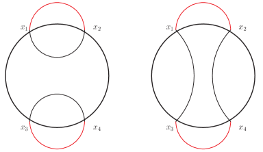
Figure 17: The full effective Wilson lines for $S$ and $U_{d}$ channels

Figure 18: The full effective Wilson lines for $T$-channel

The gauge inner product $<\psi_{2}^{G}|\psi_{1}^{G}>$ corresponding to identity matter scattering (i.e. the geodesic paths of the matter particles from prduction to annihilations) depends on the scattering channel. Let us first study scattering in the identity channel. The initial particle created at $x_{1}$ connects up to the final particle at $x_{3}$, while the particle created at $x_{2}$ connects up with the final particle at $x_{4}$. Combining with the external lines, the full effective Wilson line is topologically a circle, see the second of Fig. 17. On the other hand, in the case of particle-particle scattering, the dominant dynamical trajectories are from the initial insertion at $x_{1}$ to the final insertion at $x_{2}$ and from the initial insertion at $x_{4}$ to the final insertion at $x_{3}$. Including the external lines, the net effective Wilson line has the topology of two circles, see the first of Fig 17.

As the topology of the effective Wilson loops in the first and second of Fig. 17 differs, it follows that the gauge theory inner product (even at zero winding) is different in the two sectors. It was demonstrated by Witten in [22] that the ratio of the path integral with two circular Wilson lines to the path integral with a single circular Wilson line is infact given by

$$\frac{k\sin(\pi{\lambda_{B}})}{\pi}=N\frac{\sin(\pi{\lambda_{B}})}{\pi{\lambda_{B}}}$$

in the large $N$ limit. It follows that we should expect that

$$T_{S}=\frac{k\sin(\pi{\lambda_{B}})}{\pi}T_{U_{d}}$$ (170)

in perfect agreement with (82) (the $\delta$ function piece in (82) is presumably related to a contact term in the correlators described in this subsection).

A similar argument relates $T_{U_{e}}$ to $T_{T}$ without any relative factor, as in this case the closed Wilson lines described above has the topology of two circles in both cases.

7.5 Direct evaluation of the S-matrix in the identity channel

The fact that we were able to solve the integral equation that determines four particle scattering only for $q^{\pm}=0$ prevented us from evaluating the S-matrix in the identity channel by direct computation. For this reason we have been forced, in this section, to resort to guesswork and indirect arguments to conjecture a result for the S-matrix in the channel with identity exchange. It would, of course, be very satisfying to be able to verify our conjecture by direct computation. Unfortunately we have not succeeded in doing this. In this subsection we briefly report two potentially promising ideas for a direct evaluation.

7.5.1 Double analytic continuation

As we have already explained above, the planar graphs that evaluate $2\rightarrow 2$ scattering may be summed by an integral equation. As a technical trick to solve the integral equation, earlier in this paper we found it convenient to analytically continue momenta to Euclidean space according to the formula $p^{0}=ip^{0}_{E}$. We then proceeded to solve the integral equation in Euclidean space. In order to evaluate $T$ and $U$-channel scattering we then analytically continued the final result back to Lorentzian space by setting $p^{0}_{E}=ip^{0}$.

There is, however, a natural, inequivalent analytic continuation of the Euclidean space integral equation to Lorentzian space: the continuation

$$p^{3}=-ip^{3}_{L}$$

Under this continuation $x^{3}$ turns into a time like coordinate, while $x^{\pm}$ are complex coordinates $x^{+}\sim z$, $x^{-}\sim{\bar{z}}$ that parameterize the spatial $R^{2}$. This at first strange sounding analytic continuation has been employed with great apparent success in several studies of the thermal partition function of large $N$ Chern-Simons theories [1, 2, 7, 3, 4, 8, 9, 10, 5], a fact that suggests this analytic continuation should be taken seriously.

Under this analytic continuation a center of mass momentum with $q^{\pm}=0$ is timelike; indeed the condition $q^{\pm}=0$ is simply the assertion that the center of mass momentum points entirely in the time direction, so that in the $S$-channel we are studying scattering in the center of mass frame.

In summary, it seems plausible that the double analytic continuation of the integral equation (86) at $q^{\pm}=0$ provides a direct computational handle on the S-matrix in the identity channel.

The discussion of this subsection may seem, at first, to directly contradict (82); surely the solution of an analytically continued integral equation is simply the analytic continuation of the solution of the original equation without any factors or additional singular terms? Infact this is not the case. It turns out that the integral equation after double analytic continuation has new singularities in the integral. These singularities - which are absent in the original equation - spoil naive analytic continuation. We illustrate this complicated set of affairs in Appendix G.1.

If the central idea of this subsection is correct, then it should be possible to obtain the scattering cross section with identity exchange by solving the double analytic continued integral equation taking the new singular contributions into account. This appears to be a delicate task that we have not managed to implement.

As a warm up to the exercise suggested in this section it would be useful to rederive the ordinary non-relativistic Aharonov-Bohm equation by solving the Lippmann Schwinger equation, order by order in perturbation theory, in momentum space, perhaps at the value of the self adjoint extension parameter $w=1$ (see [21] ) at which point the Aharonov-Bohm amplitude is an analytic function of $\nu$ so perturbation theory is well-defined. We suspect that this exercise will encounter all the subtle singularities discussed in this section, and it would be useful to learn how to carefully deal with these singularities in a context where the answer is known without doubt. We postpone further study of these ideas to future work.

7.5.2 Schrodinger equation in lightfront quantization?

It is striking that in the non-relativistic limit, the exact S-matrix was obtained rather easily by solving a Schrodinger equation in position space. One might wonder if the full non-relativistic S-matrix may similarly be obtained by solving an appropriate Schrodinger equation.

An observation that supports this hope is the fact that genuine ‘particle creation’ never occurs in the large $N$ limit. A Feynman diagram that describes virtual fundamental particles being created and destroyed during a scattering process has additional index loops and is suppressed in the large $N$ limit. It thus seems plausible that the scattering matrices of interest to us in this paper may be obtained by solving the relevant quantum mechanical problem.

Although we will not present the details here, we have succeeded in reproducing the effective scattering amplitude of the ungauged large $N$ $\phi^{4}$ theory by solving a two particle Schrodinger equation. The Schrodinger equation in question is obtained from a lightcone quantization of the quantum field theory. It may well prove possible to extend this analysis to the gauged theory, and thereby extract the S-matrix from an effective Schrodinger equation; however we have not yet succeeded in implementing this idea. We leave further study of this idea to future work.

8 Discussion

In this paper we have presented computations and conjectures for the formulas for $2\rightarrow 2$ scattering in large $N$ matter Chern-Simons theories at all orders in the ’t Hooft coupling. All the computations presented in this paper were performed in the light cone gauge together with an assumption of involving the precise definition of the gauge propagator in this gauge. It would be useful to have checks of our results using different methods - perhaps working in a covariant gauge. It might be possible (and would be very interesting) to generalize the covariant computation of section 5 to two loops. It would also be very interesting to study how (and whether) the unusual structural features predicted in our paper manifest themselves in a covariant computation.

Obvious extensions of our paper include the generalization of the computations presented here to the simplest $N=2$ supersymmetric matter Chern-Simons theories, and also to the large class of single boson-fermion theories studied in [6]. It may also be possible to match the finite $b_{4}$ results of the bosonic computations in this paper with a generalized fermionic computation in which we include a $({\bar{\psi}}\psi)^{2}$ term in the fermionic Lagrangian.

Perhaps the most interesting formula presented in this paper is the formula for the scattering matrix in the $S$-channel. (see (81), (82)). This formula is manifestly unitary: it includes an unusual rescaling of the identity piece in the S-matrix; it agrees with the formula for Aharonov-Bohm scattering in the non-relativistic limit, and the formula for large $N$ $\phi^{4}$ scattering in the small ${\lambda_{B}}$ limit. It is also tightly related to scattering in the other channels via rescaled relations of crossing symmetry. In the case of the scalar theory, this S-matrix also has poles signalling the existence of a stable singlet bound state of two particles in the singlet channel over a range of values of $b_{4}$. Unfortunately the formula for $S$-channel scattering presented in this paper has not been derived but has simply been conjectured. A very important problem for the future is to honestly derive the formula for $S$-channel scattering, perhaps along the lines sketched in subsection 7.5.

Another reason to understand scattering after the double analytic continuation described in subsection 7.5 is to better understand the detailed connection between the Lorentzian results of our paper and the Euclidean results of earlier computations [1, 2, 7, 8, 9, 10, 5].

The S-matrices derived in our paper have all been obtained for the scattering of massive particles. There is no barrier to taking the high energy (or equivalently zero mass) limit of our scattering amplitudes. Interestingly, the scattering amplitudes develop no new infrared singlularities in this limit. This fact is probably an artifact of the large N limit that supresses the pair creation of fundamental particles; it seems likely that $\frac{1}{N}$ corrections to the results presented in this paper will have new infrared singularities in the zero mass limit.

As we have explained, the formulas (and conjectures) presented in this paper imply that the usual rules of crossing symmetry are modified in matter Chern-Simons theories. In this paper we have presented a conjecture for the nature of that modification in the ’t Hooft large $N$ limit. It would be interesting to prove this rule analogue of crossing symmetry (perhaps using a refinement of the arguments in subsection 7.4).

A simplifying feature of the ’t Hooft large $N$ is that scattering was truly anyonic (i.e. was characterized by a nonzero anionic phase) only in the singlet channel of Particle-antiparticle scattering. In particular the anyonic phase vanishes in particle-particle scattering (see subsection 2.6) so that we were never forced in this paper to address issues having to do with the generalization of Bose or Fermi statistics. At finite $N$ and $k$ this situation will change, presumably leading to nontrivial phases between particle-particle scattering in the direct and exchange channels. These considerations suggest that the crossing symmetry structure of scattering amplitudes will be very rich at finite $N$ and $k$; it would be fascinating to have even a well motivated conjecture for this structure. It is conceivable that the S-matrix presented in this paper and its generalization to the finite $N$ and $k$ case may have useful applications in the condensed matter problems and also in the area of the topological quantum computation [23].

If the unusual structural properties conjectured in this paper withstand further scrutiny, then they are likely to be general features of all matter Chern-Simons theories. We should, in particular, be able to probe these features in the scattering of maximally supersymmetric Chern-Simons theories (ABJ theories). In this connection it is interesting to note that there is an unresolved paradox in the study of scattering amplitudes in ABJM and ABJ theory. In this theory the $2\rightarrow 2$ scattering amplitude has been argued to vanish at one loop [24, 25, 26], but to be non vanishing at two loops [27, 28, 26]. The paradox arises because although the proposed two loop formula for four particle scattering in ABJM theory has cuts [27], there do not seem to exist any candidate intermediate processes to saturate these cuts. While scattering amplitudes in ABJ theory are more confusing than those considered in this paper because they receive infrared divergences from intermediate massless scalar and fermion propagation, it is at least conceivable that the resolution to this apparent unitarity paradox lies along the lines sketched in this paper. The results of our paper should generalize, in the most straightforward fashion, to scattering in $U(M)\times U(N)$ theory when $\frac{M}{N}<<1$ (in this limit the ABJ theory begins to closely resemble a theory with a single gauge group and only fundamental matter, like the theories studied in this paper). The analysis of our paper suggests that the $2\rightarrow 2$ scattering amplitude does not completely vanish at one loop: it should at least have a $\delta$ function localized singular piece. The contribution of this piece in a one loop sub diagram to two loop graphs could then, additionally, modify the scattering amplitudes as well as the usual rules of crossing symmetry. It would be fascinating to verify these expectations via a direct analysis of scattering amplitudes in the supersymmetric theories.

A significant check of all the computations and conjectures presented in our paper is that they are all consistent with the recently conjectured level-rank duality between bosonic and fermionic Chern-Simons theories. This works in a rather remarkable way. The bosonic S-matrices have nontrivial analytic structure (e.g. two particle cuts) at all values of $\lambda_{B}$ (including $\lambda_{B}=0$ where the cuts come from the four boson contact interaction) provided $|\lambda_{B}|\neq 1$. Precisely at $\lambda_{B}=1$, however, the bosonic S-matrix collapses into precisely the analytically trivial constant that one predicts from fermionic tree level scattering. Indeed the agreement between bosonic and fermionic S-matrices works at all values of $\lambda_{B}$, not just at extreme ends.

Indeed the results of our paper shed some additional light on the working of this duality. The first point, as we have already emphasized in the introduction, is that our S-matrix is effectively anyonic in the singlet channel. The effective anyonic phase can be estimated very simply in the non-relativistic limit, and the duality map from $\lambda_{B}$ to $\lambda_{F}$ can simply be deduced by demanding that the dual theories have equal anyonic phases.

In the $U$-channel, on the other hand, the anyonic phase is trivial. Bosonic and fermionic S matrices map to each other only after we transpose the exchange representations. As we have explained in more detail in the introduction, this suggests that, for scattering purposes, there exists a map between asymptotic multi bosonic states that transform in representation $R$ of $U(N_{B})$ and multi- fermionic states that transform in representation $R^{T}$ of $U(N_{F})$.

There is an obvious puzzle about the identification suggested above; namely the number of states on the two sides do not match (this is true even if we restrict to the simplest representation, namely the fundamental, simply because $N_{B}\neq N_{F}$). It seems possible that the duality between the bosonic and fermionic theories really works only on compact manifolds (and so, effectively, only in the singlet sector on $R^{2}$). If this turns out to be the correct eventual statement of the duality, then the perfect match under duality of the scattering amplidues in non singlet sectors may eventually find its explaination in the match of factorized subsectors in higher point scattering in the singlet channel. For instance one could consider the scattering of two particles, and simultaneously the scatering of two antiparticles very far away, with colour indices chosen so that the full four particle initial state is a singlet and so duality invariant. Presumably the scattering amplitudes factor into the scattering amplitude for particle - particle scattering and the scatterng amplitude for antiparticle-antiparticle scattering, implying the duality invariance of these more basic 2 particle scattering amplitudes, even though they do not occur in a gauge singlet sector, explaining the results obtained in this paper. It would certainly be nice to understand this better.

In summary, the results and conjectures presented in this paper have several unexpected features, have intriguing implications, and throw up several puzzles. If our results stand up to further scrutiny they suggest several fascinating new directions of investigation.

Appendix A The identity S-matrix as a function of $s$, $t$, $u$

As explained in subsection 2.3, the identity S-matrix has a simple form in the center of mass frame; it is given by

$$(2\pi)^{3}\delta^{3}(p_{1}+p_{2}-p_{3}-p_{4})8\pi\sqrt{s}\delta(\theta)$$

As we will see below, the expression $\delta(\theta)$ is slightly singular when recast in terms of invariants, so we will find it convenient to regulate this expression as

$$(2\pi)^{3}\delta^{3}(p_{1}+p_{2}-p_{3}-p_{4})4\pi\sqrt{s}\lim_{\epsilon\to 0}\left(\delta(\theta-\epsilon)+\delta(\theta+\epsilon)\right).$$

Using (23), this expression may be recast in invariant form

$$\delta\left(\sqrt{\frac{4t}{t+u}}-\epsilon\right)(2\pi)^{3}\delta^{3}(p_{1}+p_{2}-p_{3}-p_{4})$$ (171)

as we have already noted in (21).

In this Appendix we present a cumbersome but direct algebraic check that $I$ as defined in (171) coincides with $I$ defined in (20). Our strategy is as follows. We start with the expression (171), and express the arguments of the delta functions in (171) entirely in terms of the 8 variables $p_{1}^{x},p_{1}^{y},p_{2}^{x},p_{2}^{y},p_{3}^{x},p_{3}^{y},p_{4}^{x},p_{4}^{y}$ (the energies of the ingoing and outgoing particles are solved for using the on shell condition). We choose to view the resultant expression as follows. We think of $p_{1}^{x},p_{1}^{y},p_{2}^{x},p_{2}^{y}$ as fixed initial data and the remaining quantities $p_{3}^{x},p_{3}^{y},p_{4}^{x},p_{4}^{y}$ as variable scattering data. The four delta functions in (171) thus determine $p_{3}^{x},p_{3}^{y},p_{4}^{x},p_{4}^{y}$ as functions of $p_{1}^{x},p_{1}^{y},p_{2}^{x},p_{2}^{y}$. At leading order in $\epsilon$ is not difficult to explicitly determine the values for $p_{3}^{x},p_{3}^{y},p_{4}^{x},p_{4}^{y}$ obtained in this manner. We find

$$p_{3,x}=p_{1,x}\pm\epsilon a_{3,x},~{}p_{4,x}=p_{2,x}\pm\epsilon a_{4,x},~{}p_{3,y}=p_{1,y}\pm\epsilon a_{3,y},~{}p_{4,y}=p_{2,y}\pm\epsilon a_{4,y}.$$ (172)

where the four $a$ variables are obtained by solving four linear equations (the $\pm$ above corresponds to the two possibilities $\theta=\epsilon$ or $\theta=-\epsilon$ in the centre- of-mass frame). In what follows below we will not need the explicit form of the solutions for the $a$ variables, but will only need certain identities obeyed by these solutions. These identities turn out, in fact, to be three of the four equations that the $a$ variables obey. The relevant three equations are

$$\begin{split}&a_{4,x}=-a_{3,x},~{}~{}a_{4,y}=-a_{3,y},~{}~{}a_{3,x}=Ba_{3,y},\\ \text{where}\quad&B=\frac{p_{2,y}\sqrt{m^{2}+p_{1,x}^{2}+p_{1,y}^{2}}-p_{1,y}\sqrt{m^{2}+p_{2,x}^{2}+p_{2,y}^{2}}}{p_{1,x}\sqrt{m^{2}+p_{2,x}^{2}+p_{2,y}^{2}}-p_{2,x}\sqrt{m^{2}+p_{1,x}^{2}+p_{1,y}^{2}}}.\end{split}$$ (173)

Let us now return to our task of rewriting the delta function in (171) in terms of delta functions linear in $p_{3}^{x},p_{3}^{y},p_{4}^{x},p_{4}^{y}$. It follows from the usual rules for manipulating delta functions that

$$\begin{split}&\delta\left(\sqrt{\frac{4t}{t+u}}-\epsilon\right)\delta^{3}(p_{1}+p_{2}-p_{3}-p_{4})\\ &=J_{1}\delta^{2}(\overrightarrow{p}_{3}-\overrightarrow{p}_{1}+\epsilon a_{3})\delta^{2}(\overrightarrow{p}_{4}-\overrightarrow{p}_{2}+\epsilon a_{4})+J_{2}\delta^{2}(\overrightarrow{p}_{3}-\overrightarrow{p}_{1}-\epsilon a_{3})\delta^{2}(\overrightarrow{p}_{4}-\overrightarrow{p}_{2}-\epsilon a_{4})\end{split}$$ (174)

where $J_{1}$ and $J_{2}$ are the relevant Jacobians. It remains to compute these Jacobians.

The reader might naively expect that the Jacobians are independent of $a_{3}$ and $a_{4}$ in the limit $\epsilon\to 0$, but that is not the case. It is not difficult verify that, in the $\epsilon\to 0$ limit the derivatives $\frac{\partial\sqrt{\frac{4t}{t+u}}}{\partial p^{x}_{3}}$ and $\frac{\partial\sqrt{\frac{4t}{t+u}}}{\partial p^{y}_{3}}$ (which enter the expression for the Jacobians) are of the form $\frac{A}{B}$ where $A$ and $B$ are both expressions of unit homogeneity in $a_{3}$ and $a_{4}$. The ratio $\frac{A}{B}$ does not depend on the overall scale of $a_{3,x},a_{3,y}$ and $a_{4,x},a_{4,y}$, but does depend on their relative magnitudes. It turns out that the equations (LABEL:asoll) are sufficient to unambiguously determine the ratio $\frac{A}{B}$ (which turns out to be the same for the two solutions corresponding to the $\pm$ signs so that $J_{1}=J_{2}=J$) ; we find

$$J=\sqrt{s}\frac{1}{E_{1}E_{2}}$$ (175)

where $E_{i}=\sqrt{m^{2}+p_{i,x}^{2}+p_{i,y}^{2}}$ and

$$s=\sqrt{2}\sqrt{\sqrt{m^{2}+p_{1,x}^{2}+p_{1,y}^{2}}\sqrt{m^{2}+p_{2,x}^{2}+p_{2,y}^{2}}+m^{2}-p_{1,x}p_{2,x}-p_{1,y}p_{2,y}}.$$ (176)

Collecting factors, it follows that the RHS of (171) coincides with the RHS of (20) in the limit $\epsilon\to 0$.

Appendix B Tree level S-matrix

The bosonic effective action is

$$T_{B}=\frac{1}{2}\int\frac{d^{3}p}{(2\pi)^{3}}\frac{d^{3}k}{(2\pi)^{3}}\frac{d^{3}q}{(2\pi)^{3}}V(p,k,q)\phi_{i}(p+q)\bar{\phi}^{j}(-k-q)\bar{\phi}^{i}(-p)\phi_{j}(k),$$ (177)

where at tree level

$$V(p,k,q)=8\pi i\lambda\epsilon_{\mu\nu\rho}\frac{q^{\mu}p^{\nu}k^{\rho}}{(k-p)^{2}}.$$ (178)

And the fermionic effective action is

$$T_{F}=\frac{1}{2}\int\frac{d^{3}p}{(2\pi)^{3}}\frac{d^{3}k}{(2\pi)^{3}}\frac{d^{3}q}{(2\pi)^{3}}V^{\alpha\gamma}_{\beta\delta}(p,k,q)\psi_{i,\alpha}(p+q)\bar{\psi}^{j,\beta}(-k-q)\bar{\psi}^{i,\delta}(-p)\psi_{j,\gamma}(k),$$ (179)

where at tree level

$$V^{\alpha\gamma}_{\beta\delta}(p,k,q)=2i\pi\lambda\epsilon_{\mu\nu\rho}\frac{(\gamma^{\mu})^{\alpha}_{\beta}(\gamma^{\nu})^{\gamma}_{\delta}(k-p)^{\rho}}{(k-p)^{2}}.$$ (180)

The gauge field propagator that we work with in this section is

$$\langle A_{\mu}(p)A_{\nu}(-q)\rangle=(2\pi)^{3}\delta^{3}(p-q)\frac{4\pi}{p^{2}}\epsilon_{\mu\nu\rho}p^{\rho}.$$ (181)

B.1 Particle-particle scattering

According to the momentum assignments in (37), The bosonic S-matrix is given by

$$\begin{split}&S_{B}(p_{1},p_{2},p_{3},p_{4})\\ =&\langle out|1+iT_{B}|in\rangle\\ =&\langle 0|a_{n}(p_{4})a_{m}(p_{3})a^{b\dagger}(p_{2})a^{a\dagger}(p_{1})|0\rangle\\ &+\frac{i}{2}\int\frac{d^{3}p}{(2\pi)^{3}}\frac{d^{3}k}{(2\pi)^{3}}\frac{d^{3}q}{(2\pi)^{3}}\Biggl{[}V(p,k,q)\\ &~{}~{}~{}~{}~{}~{}~{}~{}\times\langle 0|a_{n}(p_{4})a_{m}(p_{3})\left(\phi_{i}(p+q)\bar{\phi}^{j}(-k-q)\bar{\phi}^{i}(-p)\phi_{j}(k)\right)a^{b\dagger}(p_{2})a^{a\dagger}(p_{1})|0\rangle\Biggr{]}.\end{split}$$ (182)

Using appropriate contractions and commutation relations, we find

$$\begin{split}S_{B}(p_{1},p_{2},p_{3},p_{4})&=\delta^{a}_{m}\delta^{b}_{n}\left(I(p_{1},p_{2},p_{3},p_{4})+iV(-p_{3},p_{2},p_{1}+p_{3})\right)\\ &+\delta^{a}_{n}\delta^{b}_{m}\left(I(p_{1},p_{2},p_{4},p_{3})+iV(-p_{4},p_{2},-p_{3}-p_{2})\right)\end{split}$$ (183)

The first term is for the $U_{d}$ channel while the other is for the $U_{e}$ channel.
Whereas the fermionic S-matrix is

$$\begin{split}&S_{F}(p_{1},p_{2},p_{3},p_{4})\\ =&\langle out|1+iT_{F}|in\rangle\\ =&\langle 0|a_{n}(p_{4})a_{m}(p_{3})a^{b\dagger}(p_{2})a^{a\dagger}(p_{1})|0\rangle\\ &+\frac{i}{2}\int\frac{d^{3}p}{(2\pi)^{3}}\frac{d^{3}k}{(2\pi)^{3}}\frac{d^{3}q}{(2\pi)^{3}}\Biggl{[}V^{\alpha\gamma}_{\beta\delta}(p,k,q)\\ &~{}~{}~{}~{}\times\langle 0|a_{n}(p_{4})a_{m}(p_{3})\left(\psi_{i,\alpha}(p+q)\bar{\psi}^{j,\beta}(-(k+q))\bar{\psi}^{i,\delta}(-p)\psi_{j,\gamma}(k)\right)a^{b\dagger}(p_{2})a^{a\dagger}(p_{1})|0\rangle\Biggr{]}\end{split}$$ (184)

Using appropriate contractions and anticommutation relations,

$$\begin{split}&S_{F}(p_{1},p_{2},p_{3},p_{4})\\ =&-\delta^{a}_{m}\delta^{b}_{n}I(p_{1},p_{2},p_{3},p_{4})\\ &-i\delta^{a}_{m}\delta^{b}_{n}V^{\alpha\gamma}_{\beta\delta}(-p_{3},p_{2},p_{1}+p_{3})\bar{u}^{\beta}(-p_{4})\bar{u}^{\delta}(-p_{3})u_{\alpha}(p_{1})u_{\gamma}(p_{2})\\ &+\delta^{a}_{n}\delta^{b}_{m}I(p_{1},p_{2},p_{4},p_{3})\\ &+i\delta^{a}_{n}\delta^{b}_{m}V^{\alpha\gamma}_{\beta\delta}(-p_{4},p_{2},-p_{3}-p_{2})\bar{u}^{\beta}(-p_{3})\bar{u}^{\delta}(-p_{4})u_{\alpha}(p_{1})u_{\gamma}(p_{2})\end{split}$$ (185)

Again, the first term is for the $U_{d}$ channel while the other is for the $U_{e}$ channel.

B.2 Particle-antiparticle scattering

According to the momentum assignments in (32), The bosonic S-matrix is given by

$$\begin{split}&S_{B}(p_{1},p_{2},p_{3},p_{4})\\ =&\langle out|1+iT_{B}|in\rangle\\ =&\langle 0|b^{n}(p_{4})a_{m}(p_{3})b_{b}^{\dagger}(p_{2})a^{a\dagger}(p_{1})|0\rangle\\ &+\frac{i}{2}\int\frac{d^{3}p}{(2\pi)^{3}}\frac{d^{3}k}{(2\pi)^{3}}\frac{d^{3}q}{(2\pi)^{3}}\Biggl{[}V(p,k,q)\\ &~{}~{}~{}~{}~{}\times\langle 0|b^{n}(p_{4})a_{m}(p_{3})\left(\phi_{i}(p+q)\bar{\phi}^{j}(-k-q)\bar{\phi}^{i}(-p)\phi_{j}(k)\right)b_{b}^{\dagger}(p_{2})a^{a\dagger}(p_{1})|0\rangle\Biggr{]}\end{split}$$ (186)

Using appropriate contractions and commutation relations, we find

$$\begin{split}S_{B}(p_{1},p_{2},p_{3},p_{4})&=\left(\delta^{a}_{m}\delta_{b}^{n}-\frac{\delta^{n}_{m}\delta_{b}^{a}}{N}\right)\left(I(p_{1},p_{2},p_{3},p_{4})+iV(-p_{3},p_{4},p_{1}+p_{3})\right)\\ &+\frac{\delta^{n}_{m}\delta_{b}^{a}}{N}\left(I(p_{1},p_{2},p_{3},p_{4})+iV(-p_{2},p_{4},p_{1}+p_{2})\right)\end{split}$$ (187)

The first term is for the $T$-channel while the other is for the $S$-channel.
Whereas the fermionic S-matrix is

$$\begin{split}&S_{F}(p_{1},p_{2},p_{3},p_{4})=\langle out|1+iT_{F}|in\rangle=\langle 0|b^{n}(p_{4})a_{m}(p_{3})b_{b}^{\dagger}(p_{2})a^{a\dagger}(p_{1})|0\rangle\\ &+\frac{i}{2}\int\frac{d^{3}p}{(2\pi)^{3}}\frac{d^{3}k}{(2\pi)^{3}}\frac{d^{3}q}{(2\pi)^{3}}V^{\alpha\gamma}_{\beta\delta}(p,k,q)\langle 0|b^{n}(p_{4})a_{m}(p_{3})\\ &\Bigg{(}\psi_{i,\alpha}(p+q)\bar{\psi}^{j,\beta}(-k-q)\bar{\psi}^{i,\delta}(-p)\psi_{j,\gamma}(k)\Bigg{)}b_{b}^{\dagger}(p_{2})a^{a\dagger}(p_{1})|0\rangle\end{split}$$ (188)

Using appropriate contractions and anticommutation relations, we find

$$\begin{split}&S_{F}(p_{1},p_{2},p_{3},p_{4})\\ &=-\left(\delta^{a}_{m}\delta_{b}^{n}-\frac{\delta^{n}_{m}\delta_{b}^{a}}{N}\right)\left(I(p_{1},p_{2},p_{3},p_{4})-iV^{\alpha\gamma}_{\beta\delta}(-p_{3},p_{4},p_{1}+p_{3})\bar{u}^{\beta}(-p_{3})\bar{v}^{\delta}(p_{2})u_{\alpha}(p_{1})v_{\gamma}(-p_{4})\right)\\ &-\frac{\delta^{n}_{m}\delta_{b}^{a}}{N}\left(I(p_{1},p_{2},p_{3},p_{4})+iV^{\alpha\gamma}_{\beta\delta}(-p_{2},p_{4},p_{1}+p_{2})\bar{v}^{\beta}(p_{2})\bar{u}^{\delta}(-p_{3})u_{\alpha}(p_{1})v_{\gamma}(-p_{4})\right)\end{split}$$ (189)

Again, the first term is for the $T$-channel while the other is for the $S$-channel.

B.3 Explicit tree level computation

Now we substitute for the $V$s for the respective channels in bosonic case, and obtain

While the fermionic expressions for $S$, $T$, $U_{d}$ and $U_{e}$ channels are (with respect to the identity) respectively,

$$\begin{split}&T_{S}=\frac{2i\pi}{k_{F}(p_{2}+p_{4})^{2}}\epsilon_{\mu\nu\rho}\left(\bar{u}(-p_{3})\gamma^{\mu}u(p_{1})\right)\left(\bar{v}(p_{2})\gamma^{\mu}v(-p_{4})\right)(p_{2}+p_{4})^{\rho}\\ &T_{T}=-\frac{2i\pi}{k_{F}(p_{3}-p_{4})^{2}}\epsilon_{\mu\nu\rho}\left(\bar{v}(p_{2})\gamma^{\mu}u(p_{1})\right)\left(\bar{u}(-p_{3})\gamma^{\mu}v(-p_{4})\right)(p_{3}+p_{4})^{\rho}\\ &T_{U_{d}}=\frac{2i\pi}{k_{F}(p_{2}+p_{3})^{2}}\epsilon_{\mu\nu\rho}\left(\bar{u}(-p_{4})\gamma^{\mu}u(p_{1})\right)\left(\bar{u}(-p_{3})\gamma^{\mu}u(p_{2})\right)(p_{2}+p_{3})^{\rho}\\ &T_{U_{d}}=\frac{2i\pi\lambda_{F}}{(p_{2}+p_{4})^{2}}\epsilon_{\mu\nu\rho}\left(\bar{u}(-p_{3})\gamma^{\mu}u(p_{1})\right)\left(\bar{u}(-p_{4})\gamma^{\mu}u(p_{2})\right)(p_{2}+p_{4})^{\rho}\end{split}$$ (190)

These expressions can be manipulated conveniently using the Gordon Identities which are derived below:
The Dirac equation satisfied by $u(p),{\bar{u}(p)},v(p),{\bar{v}(p)}$ are given by

$$\begin{split}&\left(i\gamma^{\mu}p_{\mu}+m\right)u(p)=0,~{}~{}{\bar{u}(p)}\left(i\gamma^{\mu}p_{\mu}+m\right)=0,\\ &\left(-i\gamma^{\mu}p_{\mu}+m\right)v(p)=0,~{}~{}{\bar{v}(p)}\left(-i\gamma^{\mu}p_{\mu}+m\right)=0.\end{split}$$ (191)

The gamma matrices are given by

$$\begin{split}\gamma^{0}=\left(\begin{array}[]{cc}0&1\\ -1&0\end{array}\right),\\ \gamma^{1}=\left(\begin{array}[]{cc}0&1\\ 1&0\end{array}\right),\\ \gamma^{2}=\left(\begin{array}[]{cc}1&0\\ 0&-1\end{array}\right).\\ \end{split}$$ (192)

They satisfy

$$\gamma^{\mu}\gamma^{\nu}=g^{\mu\nu}-\epsilon^{\mu\nu\rho}\gamma_{\rho}.$$ (193)

Now, using Dirac equation (191), it is easy derive the Gordon identities

$$\begin{split}-{\bar{u}}(p_{1})\gamma^{\mu}u(p_{2})&=i\left({\bar{u}}(p_{1})\frac{(p_{1}+p_{2})^{\mu}}{2m}u(p_{2})-\epsilon^{\mu\nu\rho}\frac{(-p_{1}+p_{2})_{\nu}}{2m}{\bar{u}}(p_{1})\gamma_{\rho}u(p_{2})\right)\\ -{\bar{u}}(p_{1})\gamma^{\mu}v(p_{2})&=i\left({\bar{u}}(p_{1})\frac{(p_{1}-p_{2})^{\mu}}{2m}v(p_{2})+\epsilon^{\mu\nu\rho}\frac{(p_{1}+p_{2})_{\nu}}{2m}{\bar{u}}(p_{1})\gamma_{\rho}v(p_{2})\right)\\ -{\bar{v}}(p_{1})\gamma^{\mu}u(p_{2})&=i\left({\bar{v}}(p_{1})\frac{(-p_{1}+p_{2})^{\mu}}{2m}u(p_{2})-\epsilon^{\mu\nu\rho}\frac{(p_{1}+p_{2})_{\nu}}{2m}{\bar{v}}(p_{1})\gamma_{\rho}u(p_{2})\right)\\ -{\bar{v}}(p_{1})\gamma^{\mu}v(p_{2})&=i\left(-{\bar{v}}(p_{1})\frac{(p_{1}+p_{2})^{\mu}}{2m}v(p_{2})+\epsilon^{\mu\nu\rho}\frac{(p_{1}+p_{2})_{\nu}}{2m}{\bar{v}}(p_{1})\gamma_{\rho}v(p_{2})\right)\end{split}$$ (194)

Using this, it is easy to show that

$$\begin{split}{\bar{u}}(p_{1})\gamma^{\mu}u(p_{2})&=\frac{1}{1+(\frac{p_{1}-p_{2}}{2m})^{2}}\left(-i\frac{(p_{1}+p_{2})^{\mu}}{2m}-\frac{1}{2m^{2}}\epsilon^{\mu\nu\rho}(p_{1})_{\nu}(p_{2})_{\rho}\right){\bar{u}}(p_{1})u(p_{2})\\ {\bar{v}}(p_{1})\gamma^{\mu}u(p_{2})&=\frac{1}{1+(\frac{p_{1}+p_{2}}{2m})^{2}}\left(-i\frac{(-p_{1}+p_{2})^{\mu}}{2m}+\frac{1}{2m^{2}}\epsilon^{\mu\nu\rho}(p_{1})_{\nu}(p_{2})_{\rho}\right){\bar{v}}(p_{1})u(p_{2})\\ {\bar{u}}(p_{1})\gamma^{\mu}v(p_{2})&=\frac{1}{1+(\frac{p_{1}+p_{2}}{2m})^{2}}\left(-i\frac{(p_{1}-p_{2})^{\mu}}{2m}+\frac{1}{2m^{2}}\epsilon^{\mu\nu\rho}(p_{1})_{\nu}(p_{2})_{\rho}\right){\bar{u}}(p_{1})v(p_{2})\\ {\bar{v}}(p_{1})\gamma^{\mu}v(p_{2})&=\frac{1}{1+(\frac{p_{1}-p_{2}}{2m})^{2}}\left(i\frac{(p_{1}+p_{2})^{\mu}}{2m}-\frac{1}{2m^{2}}\epsilon^{\mu\nu\rho}(p_{1})_{\nu}(p_{2})_{\rho}\right){\bar{v}}(p_{1})v(p_{2})\\ \end{split}$$ (195)

The only thing that is remaining is to compute the quantities, ${\bar{u}}(p^{\prime})u(p),{\bar{v}}(p^{\prime})v(p),{\bar{u}}(p^{\prime})v(p),{\bar{v}}(p^{\prime})u(p).$ For this, we explicitly construct the solution for $V$ and $u$ starting boosting the rest frame results which are easily computable to a frame where the momenta is $p.$ In the rest frame, equation satisfied by the $u$ and $v$ is given by,

$$\left(-i\gamma^{0}+I\right)u(0)=0,~{}~{}~{}\left(i\gamma^{0}+I\right)v(0)=0,$$ (196)

and for ${\bar{u}}$ and ${\bar{v}}$

$${\bar{u}}(0)\left(-i\gamma^{0}+I\right)=0,~{}~{}~{}{\bar{v}}(0)\left(i\gamma^{0}+I\right)=0,$$ (197)

where $I$ denotes, the $2\times 2$ identity matrix. The solutions are

$$u(0)=\sqrt{m}\left(1,-i\right),~{}~{}v(0)=\sqrt{m}\left(1,i\right),~{}~{}{\bar{u}}(0)=\sqrt{m}\left(1,i\right),~{}~{}{\bar{v}}(0)=\sqrt{m}\left(-1,i\right).$$ (198)

Suppose we are now interested in solution for $u$ and $v$ at momenta $p,$ given by

$$p_{\mu}=\left(-m\cosh(\alpha),m\sinh(\alpha)\cos(\theta),m\sinh(\alpha)\sin(\theta)\right).$$ (199)

The solutions are given by

$$\begin{split}u(p)&=\left(\cosh(\frac{\alpha}{2})I-\sinh(\frac{\alpha}{2})\left(\cos(\theta)\gamma^{2}-\sin(\theta)\gamma^{1}\right)\right)u(0)\\ {\bar{u}}(p)&={\bar{u}}(0)\left(\cosh(\frac{\alpha}{2})I+\sinh(\frac{\alpha}{2})\left(\cos(\theta)\gamma^{2}-\sin(\theta)\gamma^{1}\right)\right)\\ v(p)&=\left(\cosh(\frac{\alpha}{2})I-\sinh(\frac{\alpha}{2})\left(\cos(\theta)\gamma^{2}-\sin(\theta)\gamma^{1}\right)\right)v(0)\\ {\bar{v}}(p)&={\bar{v}}(0)\left(\cosh(\frac{\alpha}{2})I+\sinh(\frac{\alpha}{2})\left(\cos(\theta)\gamma^{2}-\sin(\theta)\gamma^{1}\right)\right).\end{split}$$ (200)

It is now easy to compute ${\bar{u}}(p^{\prime})u(p),{\bar{v}}(p^{\prime})v(p),{\bar{u}}(p^{\prime})v(p),{\bar{v}}(p^{\prime})u(p).$ Results are given by

$$\begin{split}{\bar{u}}(p_{1})u(p_{2})=&e^{i\tan^{-1}\frac{\sin(\theta_{2}-\theta_{1})}{\cos\left(\theta_{2}-\theta_{1}\right)-\coth(\alpha_{1})\coth(\alpha_{2})}}\sqrt{\left(2m^{2}-2~{}p_{1}\cdot p_{2}\right)},\\ {\bar{v}}(p_{1})v(p_{2})=&e^{i\tan^{-1}\frac{\sin(\theta_{1}-\theta_{2})}{\cos\left(\theta_{1}-\theta_{2}\right)-\coth(\alpha_{1})\coth(\alpha_{2})}}\sqrt{\left(2m^{2}-2~{}p_{1}\cdot p_{2}\right)},\\ {\bar{v}}(p_{1})u(p_{2})=&e^{i\tan^{-1}\frac{\sinh\left(\frac{\alpha_{1}}{2}\right)\cosh\left(\frac{\alpha_{2}}{2}\right)\sin\left(\theta_{1}\right)-\sinh\left(\frac{\alpha_{2}}{2}\right)\cosh\left(\frac{\alpha_{1}}{2}\right)\sin\left(\theta_{2}\right)}{\sinh\left(\frac{\alpha_{1}}{2}\right)\cosh\left(\frac{\alpha_{2}}{2}\right)\cos\left(\theta_{1}\right)-\sinh\left(\frac{\alpha_{2}}{2}\right)\cosh\left(\frac{\alpha_{1}}{2}\right)\cos\left(\theta_{2}\right)}}\\ &\times\sqrt{\left(-2m^{2}-2~{}p_{1}\cdot p_{2}\right)},\\ {\bar{u}}(p_{1})v(p_{2})=&e^{i\tan^{-1}\frac{\sinh\left(\frac{\alpha_{2}}{2}\right)\cosh\left(\frac{\alpha_{1}}{2}\right)\sin\left(\theta_{2}\right)-\sinh\left(\frac{\alpha_{1}}{2}\right)\cosh\left(\frac{\alpha_{2}}{2}\right)\sin\left(\theta_{1}\right)}{\sinh\left(\frac{\alpha_{1}}{2}\right)\cosh\left(\frac{\alpha_{2}}{2}\right)\cos\left(\theta_{1}\right)-\sinh\left(\frac{\alpha_{2}}{2}\right)\cosh\left(\frac{\alpha_{1}}{2}\right)\cos\left(\theta_{2}\right)}}\\ &\times\sqrt{\left(-2m^{2}-2~{}p_{1}\cdot p_{2}\right)},\\ \end{split}$$ (201)

As a final ingredient to compute the tree level scattering is

$$\begin{split}&\epsilon_{\mu\nu\rho}{\bar{u}}(p_{1})\gamma^{\mu}u(p_{2}){\bar{u}}(p_{3})\gamma^{\nu}u(p_{4})p_{5}^{\rho}\\ =&\frac{\left({\bar{u}}(p_{1})u(p_{2})\right)\left({\bar{u}}(p_{3})u(p_{4})\right)}{\left(1+\frac{(p_{1}-p_{2})^{2}}{4m^{2}}\right)\left(1+\frac{(p_{3}-p_{4})^{2}}{4m^{2}}\right)}\\ &~{}\times\Big{[}-\frac{1}{4m^{2}}\epsilon_{\mu\nu\rho}(p_{1}+p_{2})^{\mu}(p_{3}+p_{4})^{\nu}p_{5}^{\rho}\\ &~{}~{}~{}~{}~{}~{}+\frac{1}{4m^{4}}\left((p_{1}\cdot p_{5})\epsilon_{\mu\nu\rho}p_{2}^{\mu}p_{3}^{\nu}p_{4}^{\rho}-(p_{2}\cdot p_{5})\epsilon_{\mu\nu\rho}p_{1}^{\mu}p_{3}^{\nu}p_{4}^{\rho}\right)\\ &~{}~{}~{}~{}~{}~{}+\frac{i}{4m^{3}}\biggl{(}(p_{4}\cdot p_{5})\left(p_{3}\cdot(p_{1}+p_{2})\right)-(p_{3}\cdot p_{5})\left(p_{4}\cdot(p_{1}+p_{2})\right)\biggr{)}\\ &~{}~{}~{}~{}~{}~{}+\frac{i}{4m^{3}}\biggl{(}(p_{1}\cdot p_{5})\left(p_{2}\cdot(p_{3}+p_{4})\right)-(p_{2}\cdot p_{5})\left(p_{1}\cdot(p_{3}+p_{4})\right)\biggr{)}\Big{]},\end{split}$$ (202)

where $p\cdot p^{\prime}=p_{\mu}p^{\prime\mu}.$ Now just by few interchange of signs, as it follows from (195), one can compute tree level with any appropriate combinatios of $u^{\prime}s$ and $v^{\prime}s$ using (201). For example,

$$\begin{split}&\epsilon_{\mu\nu\rho}{\bar{v}}(p_{1})\gamma^{\mu}v(p_{2}){\bar{u}}(p_{3})\gamma^{\nu}u(p_{4})p_{5}^{\rho}\\ =&\frac{\left({\bar{v}}(p_{1})v(p_{2})\right)\left({\bar{u}}(p_{3})u(p_{4})\right)}{\left(1+\frac{(p_{1}-p_{2})^{2}}{4m^{2}}\right)\left(1+\frac{(p_{3}-p_{4})^{2}}{4m^{2}}\right)}\\ &~{}\times\Big{[}\frac{1}{4m^{2}}\epsilon_{\mu\nu\rho}(p_{1}+p_{2})^{\mu}(p_{3}+p_{4})^{\nu}p_{5}^{\rho}\\ &~{}~{}~{}~{}~{}~{}+\frac{1}{4m^{4}}\left((p_{1}\cdot p_{5})\epsilon_{\mu\nu\rho}p_{2}^{\mu}p_{3}^{\nu}p_{4}^{\rho}-(p_{2}\cdot p_{5})\epsilon_{\mu\nu\rho}p_{1}^{\mu}p_{3}^{\nu}p_{4}^{\rho}\right)\\ &~{}~{}~{}~{}~{}~{}+\frac{i}{4m^{3}}\left(-(p_{4}\cdot p_{5})\left(p_{3}\cdot(p_{1}+p_{2})\right)+(p_{3}\cdot p_{5})\left(p_{4}\cdot(p_{1}+p_{2})\right)\right)\\ &~{}~{}~{}~{}~{}~{}+\frac{i}{4m^{3}}\left((p_{1}\cdot p_{5})\left(p_{2}\cdot(p_{3}+p_{4})\right)-(p_{2}\cdot p_{5})\left(p_{1}\cdot(p_{3}+p_{4})\right)\right)\Big{]}.\end{split}$$ (203)

Using formulas presented in (LABEL:uchng), (LABEL:tchng) we find

$$\begin{split}{\bf S}_{F,U_{d}}&=-I(p_{1},p_{2},p_{3},p_{4})-e^{i\alpha_{1}}\frac{8\pi}{k_{F}}\left(\frac{\epsilon_{\mu\nu\rho}p_{1}^{\mu}p_{2}^{\nu}p_{3}^{\rho}}{(p_{2}+p_{3})^{2}}-2im_{F}\right)(2\pi)^{3}\delta(p_{1}+p_{2}+p_{3}+p_{4}),\\ {\bf S}_{F,U_{e}}&=I(p_{1},p_{2},p_{4},p_{3})-e^{i\alpha_{2}}\frac{8\pi}{k_{F}}\left(\frac{\epsilon_{\mu\nu\rho}p_{1}^{\mu}p_{2}^{\nu}p_{3}^{\rho}}{(p_{2}+p_{4})^{2}}+2im_{F}\right)(2\pi)^{3}\delta(p_{1}+p_{2}+p_{3}+p_{4}),\\ {\bf S}_{F,T}&=-I(p_{1},p_{2},p_{3},p_{4})+e^{i\alpha_{3}}\frac{8\pi}{k_{F}}\left(\frac{\epsilon_{\mu\nu\rho}p_{1}^{\mu}p_{2}^{\nu}p_{3}^{\rho}}{(p_{4}+p_{3})^{2}}+2im_{F}\right)(2\pi)^{3}\delta(p_{1}+p_{2}+p_{3}+p_{4}),\\ {\bf S}_{F,S}&=-I(p_{1},p_{2},p_{3},p_{4})+e^{i\alpha_{4}}8\pi\lambda_{F}\left(\frac{\epsilon_{\mu\nu\rho}p_{1}^{\mu}p_{2}^{\nu}p_{3}^{\rho}}{(p_{2}+p_{4})^{2}}-2im_{F}\right)(2\pi)^{3}\delta(p_{1}+p_{2}+p_{3}+p_{4}),\end{split}$$ (204)

where $\alpha_{1}$ to $\alpha_{4}$ are some complicated physically irelevant phase factors. They obey interchange symmetry and for equal momneta (for example, in (201), $p_{1}=p_{2}$) phase vanishes. In particular, this implies that the phase factor in $U_{d}$ and $U_{e}$ channel are the same. Although, these phases has no physical relevance, we present the results in the C.M. frame. Let the incoming momenta be $p_{1},p_{2}$ and out going momenta are $-p_{3},-p_{4}$ and the angle between $p_{1}$ and $-p_{3}$ is given by $\theta$ then we find $\alpha_{1}=\alpha_{2}=\alpha_{3}=\alpha_{4}=-\theta.$ Note that, inparticular this has the property that, near identity, phase factors has no contribution, this is what we expect also from physical ground. So the answers obey the duality with the Bosonic answers in the respective channels.
For completeness, we also write answers for bosonic case.

$$\begin{split}{\bf S}_{B,U_{d}}&=I(p_{1},p_{2},p_{3},p_{4})-\frac{8\pi}{k_{B}}\frac{\epsilon_{\mu\nu\rho}p_{1}^{\mu}p_{2}^{\nu}p_{3}^{\rho}}{(p_{2}+p_{3})^{2}}(2\pi)^{3}\delta(p_{1}+p_{2}+p_{3}+p_{4})\\ {\bf S}_{B,U_{e}}&=I(p_{1},p_{2},p_{4},p_{3})+\frac{8\pi}{k_{B}}\frac{\epsilon_{\mu\nu\rho}p_{1}^{\mu}p_{2}^{\nu}p_{3}^{\rho}}{(p_{2}+p_{4})^{2}}(2\pi)^{3}\delta(p_{1}+p_{2}+p_{3}+p_{4})\\ {\bf S}_{B,T}&=I(p_{1},p_{2},p_{3},p_{4})+\frac{8\pi}{k_{B}}\frac{\epsilon_{\mu\nu\rho}p_{1}^{\mu}p_{2}^{\nu}p_{3}^{\rho}}{(p_{4}+p_{3})^{2}}(2\pi)^{3}\delta(p_{1}+p_{2}+p_{3}+p_{4})\\ {\bf S}_{B,S}&=I(p_{1},p_{2},p_{3},p_{4})-8\pi\lambda_{B}\frac{\epsilon_{\mu\nu\rho}p_{1}^{\mu}p_{2}^{\nu}p_{3}^{\rho}}{(p_{2}+p_{4})^{2}}(2\pi)^{3}\delta(p_{1}+p_{2}+p_{3}+p_{4}).\\ \end{split}$$ (205)

Appendix C Aharonov-Bohm scattering

In this section we will review the classic computation, first performed by Aharonov and Bohm, of the scattering of a charged non-relativistic particle off a flux tube; see [18, 16, 19, 14, 20, 21] for relevant references. We assume that the flux tube is oriented in the $z$ direction, and sits at the origin of the transverse two dimensional space. We focus on states that also preserve translational invariance along the $z$ direction, so our problem is effectively two (spatial) dimensional. We assume that the integrated flux of the flux tube equals $2\pi\nu$ so that the phase associated with the charge particle circling the flux tube is $2\pi i\nu$ (the particle is assumed to carry unit charge and mass $m$). Throughout this appendix we assume $|\nu|<1$.

C.1 Derivation of the scattering wave function

We will find scattering state solutions at energy $E=\frac{k^{2}}{2m}$ of the Schrodinger equation for this particle; intuitively $k$ is the momentum of the particle incident on the flux.

The time independent Schrodinger equation that governs our system is

$$\left(-\frac{1}{2m}\left({\bf\nabla}+2\pi i\nu{\bf G}\right)^{2}-\frac{k^{2}}{2m}\right){\psi}=0$$ (206)

where

$$G_{i}=\frac{\epsilon_{ij}}{2\pi}\partial_{j}\ln r$$ (207)

In polar coordinates the one form $G$ is given by

$$G=\frac{d\phi}{2\pi}.$$

Following Aharonov and Bohm we adopt ‘regular’ boundary conditions at the origin of our space, i.e. we demand that the wave function at the origin remain finite. As we will see below this requirement forces the wave function to vanish at the origin like $r^{|}\nu|$ in the $s$ wave channel. The appearance of $|\nu|$ in this boundary condition results in a scattering amplitude that is non-analytic as a function of $\nu$ and $\nu=0$.

The most general solution to the Schrodinger equation consistent with the boundary conditions described above is given by

$$\psi(r,\theta)=\sum_{n>0}a_{n}e^{in\theta}J_{n+\nu}(kr)+\sum_{n>0}a_{-n}e^{-in\theta}J_{n-\nu}+a_{0}J_{|\nu|}(kr)$$ (208)

Recall the asymptotic expansion of Bessel functions at small and large values of the argument

$$J_{\alpha}(x)=\frac{\left(\frac{x}{2}\right)^{\alpha}}{\Gamma(\alpha+1)}+\ldots,~{}~{}~{}=\frac{1}{\sqrt{2\pi x}}\left(e^{ix-i\frac{\pi}{4}-i\frac{\alpha\pi}{2}}+e^{-ix+i\frac{\pi}{4}+i\frac{\alpha\pi}{2}}\right)$$ (209)

and the expansion of the plane wave in terms of Bessel functions

$$e^{ikx}=\sum_{n}i^{n}J_{n}(kr)e^{in\theta}$$ (210)

and the large $r$ expansion of this plane wave (obtained by substituting (208) into (210))

$$\begin{split}e^{ikx^{\prime}}&=e^{ikr^{\prime}\cos(\theta)}=\sum_{n}i^{n}e^{in\theta}J_{n}(kr)\\ \sum_{n}i^{n}e^{in\theta}J_{n}(kr)&\approx\frac{1}{\sqrt{2\pi kr}}\sum_{n}i^{n}e^{in\theta}\left((e^{ikr-\frac{i\pi n}{2}-\frac{i\pi}{4}}+e^{-ikr+\frac{i\pi n}{2}+\frac{i\pi}{4}}\right)\qquad(r\gg 1)\\ &=\frac{2\pi}{\sqrt{2\pi kr}}\left(e^{\frac{-i\pi}{4}}e^{ikr}\delta(\theta)+e^{\frac{i\pi}{4}}e^{-ikr}\delta(\theta-\pi)\right).\end{split}$$ (211)

It is easy to see that the unique solution of the form (208) whose ingoing part - i.e. part proportional to $e^{-ikr}$ - is identical to the plane wave (210) is given by

$$\psi(r,\theta)=\sum_{n=1}^{\infty}i^{n}e^{-i\frac{\pi\nu}{2}}J_{n+\nu}(kr)e^{in\theta}+\sum_{n=1}^{\infty}i^{n}e^{i\frac{\pi\nu}{2}}J_{n-\nu}(kr)e^{-in\theta}+e^{-i\frac{\pi|\nu|}{2}}J_{|\nu|}(kr)$$ (212)

C.2 The scattering amplitude

At large $r$ $\psi(r)$ reduces to

$$\frac{1}{\sqrt{2\pi kr}}\left(2\pi e^{i\frac{\pi}{4}}\delta(\theta-\pi)e^{-ikr}+H(\theta)e^{-i\frac{\pi}{4}}e^{ikr}\right)$$ (213)

where

$$H(\theta)=e^{-i\pi|\nu|}+\sum_{n=1}^{\infty}\left(e^{-i\pi\nu}e^{in\theta}+e^{i\pi\nu}e^{-in\theta}\right).$$ (214)

Decomposing $H(\theta)$ up into its even and odd parts and then further processing we find

$$\begin{split}H(\theta)&=\left(\sum_{n=1}^{\infty}2\cos(\pi\nu)\cos(n\theta)\right)+e^{-i|\nu|\pi}+\left(\sum_{n=1}^{\infty}2\sin(\pi\nu)\sin(n\theta)\right)\\ &=\left(\cos(\nu\pi)+\sum_{n=1}^{\infty}2\cos(\pi\nu)\cos(n\theta)\right)-i|\sin(\nu\pi)|+\left(\sum_{n=1}^{\infty}2\sin(\pi\nu)\sin(n\theta)\right)\\ &=2\pi\cos(\pi\nu)\delta(\theta)-i|\sin(\nu\pi)|+\left(\sum_{n=1}^{\infty}2\sin(\pi\nu)\sin(n\theta)\right)\\ &=2\pi\cos(\pi\nu)\delta(\theta)+\sin(\pi\nu){\rm Pv}\left(\cot\left(\frac{\theta}{2}\right)\right)-i|\sin(\pi\nu)|\\ &=2\pi\cos(\pi\nu)\delta(\theta)+\sin(\pi\nu){\rm Pv}\left(\frac{e^{-i\frac{\theta{\rm sgn}[\nu]}{2}}}{\sin\left(\frac{\theta}{2}\right)}\right).\\ \end{split}$$ (215)

It is conventional to write the wave function as a plane wave plus a scattered piece ; at large $r$

$$\psi(r)=e^{ikx}+\frac{h(\theta)e^{-i\frac{\pi}{4}}e^{ikr}}{\sqrt{2\pi kr}}.$$ (218)

Plugging (211) into (218) and comparing with (213) we conclude that

$$h(\theta)=H(\theta)-2\pi\delta(\theta)$$ (219)

so that

$$h(\theta)=2\pi\left(\cos(\pi\nu)-1\right)\delta(\theta)+\sin(\pi\nu){\rm Pv}\left(\frac{e^{-i\frac{\theta{\rm sgn}[\nu]}{2}}}{\sin\left(\frac{\theta}{2}\right)}\right).$$ (220)

C.3 Physical interpretation of the $\delta$ function at forward scattering

It is intuitively clear that the amplitude for propagation (path integral) for a particle starting out a large distance away from the origin on the negative real axis, to a position nearer the scattering center has enough information to compute the scattering S-matrix. The amplitude for a particle to propagate from far to the left of the origin to a point near the origin (lets say at angle $\theta\approx\pi$ for definiteness) receives contributions from path whose angular winding around the origin are approximately $...-3\pi,-\pi,\pi,3\pi...$. Of these infinitely many paths those with winding approximately $\pi$ and $-\pi$ are special. These sectors consist of paths that go below the origin, and paths that go above the origin, but do not otherwise wind the origin. It may be shown that these paths are entirely responsible for the terms in $H(\theta)$ (see the previous subsection) proportional to $\delta(\theta)$.

For a free plane wave $H(\theta)=2\pi\delta(\theta)$. In a ‘traditional’ scattering problem $H(\theta)=2\pi\delta(\theta)+{\rm nonsingular}$ i.e. the incident wave goes through largely untouched, and in addition we have some scattering. In the problem with Aharonov-Bohm scattering, however, we have seen in the last subsection that $H(\theta)=2\pi\cos(\pi\nu)\delta(\theta)$. This fact is easily interpreted. The contribution of paths with winding $\pi$ and $-\pi$ in this problem is identical to the contribution of the same paths in the free theory except that the paths with winding $\pi$ are weighted by an additional phase $e^{i\pi\nu}$ while the paths with winding $-\pi$ are weighted by the additional phase $e^{-i\pi\nu}$. The two sectors are flipped by reflection and so otherwise contribute equally. This explains the modulation of the $\delta(\theta)$ part of $H(\theta)$ by $\cos(\pi\nu)$, and the consequent appearance of the term $2\pi(\cos(\pi\nu)-1)\delta(\theta)$ in $h(\theta)$.

Appendix D Details of the computation of the scalar S-matrix

D.1 Computation of the effective one particle exchange interaction

In this subsection we explicitly compute the summation over the effective ‘one particle exchange’ four point interactions depicted in Fig 4. We perform our computation in Euclidean space and analytically continue our final result back to Euclidean space. In Figure 19 we redraw the diagrams of Fig 4, this time including detailed momentum assignments for all legs.

Figure 19: The one loop diagrams that contribute to the unit represented by the triple line excluding the tree level diagram. Note that box diagram is not included here as it is one of the contributions from two units sewn together.

.

The graph in Fig. 19 evaluates to

$$NA_{1} =(-4\pi^{2}\lambda^{2})\int-\frac{(r+p)_{-}}{(r-p)_{-}}\frac{(r+k)_{-}}{(r-k)_{-}}\frac{1}{r^{2}+c_{B}^{2}}\frac{d^{3}r}{(2\pi)^{3}}$$

$$=\int-\left(1+2\frac{(p+k)_{-}}{(p-k)_{-}}\left(\frac{p_{-}}{(r-p)_{-}}-\frac{k_{-}}{(r-k)_{-}}\right)\right)\frac{1}{r^{2}+c_{B}^{2}}\frac{d^{3}r}{(2\pi)^{3}}$$

Let $\theta$ denote the phase of the complex number $r_{-}$. Since $r^{2}$ doesn’t have a $\theta$ dependence, performing the $\theta$ integration first,

$$NA_{1}=(-4\pi^{2}\lambda^{2})\int-\left(1-2\frac{(p+k)_{-}}{(p-k)_{-}}\left(\theta(p_{s}-r_{s})-\theta(k_{s}-r_{s})\right)\right)\frac{1}{r^{2}+c_{B}^{2}}\frac{dr_{3}r_{s}dr_{s}}{(2\pi)^{2}}$$ (226)

The graph in Fig. 19 evaluates to

$$NA_{2}=(-4\pi^{2}\lambda^{2})\int-\frac{(r+p+2q)_{-}}{(r-p)_{-}}\frac{(r+k+2q)_{-}}{(r-k)_{-}}\frac{1}{(r+q)^{2}+c_{B}^{2}}\frac{d^{3}r}{(2\pi)^{3}}$$

we can change the integration variable$r\rightarrow r-q$ and define variables $p^{\prime}=p+q$,$k^{\prime}=k+q$.

$$NA_{2} =(-4\pi^{2}\lambda^{2})\int-\frac{(r+p^{\prime})_{-}}{(r-p^{\prime})_{-}}\frac{(r+k^{\prime})_{-}}{(r-k^{\prime})_{-}}\frac{1}{r^{2}+c_{B}^{2}}\frac{d^{3}r}{(2\pi)^{3}}$$

$$=\int-\left(1+2\frac{(p^{\prime}+k^{\prime})_{-}}{(p-k)_{-}}\left(\frac{p^{\prime}_{-}}{(r-p^{\prime})_{-}}-\frac{k^{\prime}_{-}}{(r-k^{\prime})_{-}}\right)\right)\frac{1}{r^{2}+c_{B}^{2}}\frac{d^{3}r}{(2\pi)^{3}}$$

Again, performing the $\theta$ integration first,

$$NA_{2}=(4\pi^{2}\lambda^{2})\int\left(1-2\frac{(p^{\prime}+k^{\prime})_{-}}{(p-k)_{-}}\left(\theta(p^{\prime}_{s}-r_{s})-\theta(k^{\prime}_{s}-r_{s})\right)\right)\frac{1}{r^{2}+c_{B}^{2}}\frac{dr_{3}r_{s}dr_{s}}{(2\pi)^{2}}$$ (227)

Fig. 19 evaluates to

$$\begin{split}NA_{3}&=(-4\pi^{2}\lambda^{2})\int-\frac{(p+k+2q)_{-}}{(p-k)_{-}}\frac{(r+k)_{-}}{(r-k)_{-}}\frac{1}{r^{2}+c_{B}^{2}}\frac{d^{3}r}{(2\pi)^{3}}\\ &=(-4\pi^{2}\lambda^{2})\int-\frac{(p^{\prime}+k^{\prime})_{-}}{(p-k)_{-}}\left(1+2\frac{k_{-}}{(r-k)_{-}}\right)\frac{1}{r^{2}+c_{B}^{2}}\frac{d^{3}r}{(2\pi)^{3}}\\ &=(-4\pi^{2}\lambda^{2})\int-\frac{(p^{\prime}+k^{\prime})_{-}}{(p-k)_{-}}\left(1-2\theta(k_{s}-r_{s})\right)\frac{1}{r^{2}+c_{B}^{2}}\frac{dr_{3}r_{s}dr_{s}}{(2\pi)^{2}}\end{split}$$ (228)

Fig. 19 evaluates to

$$\begin{split}NA_{4}&=(-4\pi^{2}\lambda^{2})\int-\frac{(p+k)_{-}}{(p-k)_{-}}\frac{(r+k+2q)_{-}}{(r-k)_{-}}\frac{1}{(r+q)^{2}+c_{B}^{2}}\frac{d^{3}r}{(2\pi)^{3}}\\ &=(-4\pi^{2}\lambda^{2})\int-\frac{(p+k)_{-}}{(p-k)_{-}}\frac{(r+k^{\prime})_{-}}{(r-k^{\prime})_{-}}\frac{1}{r^{2}+c_{B}^{2}}\frac{d^{3}r}{(2\pi)^{3}}\\ &=(-4\pi^{2}\lambda^{2})\int-\frac{(p+k)_{-}}{(p-k)_{-}}\left(1+2\frac{k^{\prime}_{-}}{(r-k^{\prime})_{-}}\right)\frac{1}{r^{2}+c_{B}^{2}}\frac{d^{3}r}{(2\pi)^{3}}\\ &=(-4\pi^{2}\lambda^{2})\int-\frac{(p+k)_{-}}{(p-k)_{-}}\left(1-2\theta(k^{\prime}_{s}-r_{s})\right)\frac{1}{r^{2}+c_{B}^{2}}\frac{dr_{3}r_{s}dr_{s}}{(2\pi)^{2}}\end{split}$$ (229)

Fig. 19 evaluates to

$$\begin{split}NA_{5}&=(-4\pi^{2}\lambda^{2})\int\frac{(p+k+2q)_{-}}{(p-k)_{-}}\frac{(r+p)_{-}}{(r-p)_{-}}\frac{1}{r^{2}+c_{B}^{2}}\frac{d^{3}r}{(2\pi)^{3}}\\ &=(-4\pi^{2}\lambda^{2})\int\frac{(p^{\prime}+k^{\prime})_{-}}{(p-k)_{-}}\left(1+2\frac{p_{-}}{(r-p)_{-}}\right)\frac{1}{r^{2}+c_{B}^{2}}\frac{d^{3}r}{(2\pi)^{3}}\\ &=(-4\pi^{2}\lambda^{2})\int\frac{(p^{\prime}+k^{\prime})_{-}}{(p-k)_{-}}\left(1-2\theta(p_{s}-r_{s})\right)\frac{1}{r^{2}+c_{B}^{2}}\frac{dr_{3}r_{s}dr_{s}}{(2\pi)^{2}}\end{split}$$ (230)

Fig. 19 evaluates to

$$\begin{split}NA_{6}&=(-4\pi^{2}\lambda^{2})\int\frac{(p+k)_{-}}{(p-k)_{-}}\frac{(r+p+2q)_{-}}{(r-p)_{-}}\frac{1}{(r+q)^{2}+c_{B}^{2}}\frac{d^{3}r}{(2\pi)^{3}}\\ &=(-4\pi^{2}\lambda^{2})\int-\frac{(p+k)_{-}}{(p-k)_{-}}\frac{(r+p^{\prime})_{-}}{(r-p^{\prime})_{-}}\frac{1}{r^{2}+c_{B}^{2}}\frac{d^{3}r}{(2\pi)^{3}}\\ &=(-4\pi^{2}\lambda^{2})\int\frac{(p+k)_{-}}{(p-k)_{-}}\left(1+2\frac{p^{\prime}_{-}}{(r-p^{\prime})_{-}}\right)\frac{1}{r^{2}+c_{B}^{2}}\frac{d^{3}r}{(2\pi)^{3}}\\ &=(-4\pi^{2}\lambda^{2})\int\frac{(p+k)_{-}}{(p-k)_{-}}\left(1-2\theta(p^{\prime}_{s}-r_{s})\right)\frac{1}{r^{2}+c_{B}^{2}}\frac{dr_{3}r_{s}dr_{s}}{(2\pi)^{2}}\end{split}$$ (231)

The total Amplitude is

$$NA_{tot}=\sum_{i=1}^{6}A_{i}$$ (232)

Which gives

$$\begin{split}NA_{tot}=\int&\frac{dr_{3}r_{s}dr_{s}}{(2\pi)^{2}}\biggl{[}\frac{(-4\pi^{2}\lambda^{2})}{r^{2}+c_{B}^{2}}\\ &\times\left(-2+\frac{4q_{-}}{(p-k)_{-}}\left[\theta(p^{\prime}_{s}-r_{s})-\theta(k^{\prime}_{s}-r_{s})+\theta(k_{s}-r_{s})-\theta(p_{s}-r_{s})\right]\right)\biggr{]}\end{split}$$ (233)

Where we recall that

$$p^{\prime}=p+q,~{}~{}~{}k^{\prime}=k+q.$$

We are interested in the special case $q^{\pm}=0$. In this case the $p^{\prime}_{\pm}=p_{\pm}$ and $k^{\prime}_{\pm}=k_{\pm}$, and so $k^{\prime}s=k_{s}$ and $p^{\prime}_{s}=p_{s}$. It follows that the $\theta$ functions in (233) cancel in pairs and

$$NA_{tot} =(-2)(-4\pi^{2}\lambda^{2})\int\frac{1}{r^{2}+c_{B}^{2}}\frac{dr_{3}r_{s}dr_{s}}{(2\pi)^{2}}$$

$$=8\pi^{2}\lambda^{2}\int\frac{1}{r^{2}+c_{B}^{2}}\frac{d^{3}r}{(2\pi)^{3}}$$ (234)

We use dimensional regularization, which replaces the integral by ($\frac{m}{4\pi}$). So ultimately these diagrams give

$$NA_{loop}=2\pi\lambda^{2}c_{B}$$ (235)

D.2 Euclidean rotation

The integral equation (90) may be used to solve for the function $V(p^{0},{\vec{p}},k^{0},{\vec{k}},q^{3})$. In this subsection we will be interested only in the dependence of $V$ on $p^{0}$ and $k^{0}$ and so use the notation $V=V(p^{0},k^{0})$.

As is often the case in the study of relativistic scattering amplitudes, in this paper we will find it convenient determine $V$ by first computing its ‘Euclidean continuation’. In this brief subsection we pause to define the Euclidean continuation of $V$, and to determine the integral equation it obeys.

Given the amplitude $V(p^{0},k^{0})$ we define the one parameter set of amplitudes, $V_{\alpha}(p^{0},k^{0})$ for $0\leq\alpha\leq\frac{\pi}{2}$ as follows. Let us assume that $V(p^{0},k^{0})$ admits an analytic continuation to the function $V(z,w)$ for $0<Arg(z)<\frac{\pi}{2}$ and $0<Arg(w)<\frac{\pi}{2}$. We also assume that this function can be defined to be free of singularities when $Arg(z)=Arg(w)$. In terms of this analytic function, we define a one parameter extension, $V_{\alpha}$ of $V$ by

$$V_{\alpha}(p^{0},k^{0})=V(p^{0}e^{i\alpha},k^{0}e^{i\alpha}).$$

It follows in particular that $V_{\alpha}$ is a smooth function of $\alpha$.

The Euclidean continuation, $V_{E}$ of $V$ is defined by

$$V_{E}(p^{0},q^{0})=V_{\frac{\pi}{2}}(p^{0},k^{0}).$$

Note in particular that

$$V_{E}(p^{0},k^{0})=V(ip^{0},ik^{0})$$

In order to obtain the integral equation obeyed by $V_{\alpha}(p^{0},q^{0})$ one must, of course, make the replacement $p^{0}\rightarrow e^{i\alpha}p^{0}$, $k^{0}\rightarrow e^{i\alpha}k^{0}$ in (34). However this replacement must also be accompanied by a simultaneous change in the contour of integration of the variable $r^{0}$. If the $r^{0}$ contour is left unchanged then the pole

$$\frac{1}{(p-r)_{+}(p-r)_{-}-i\epsilon}$$

in the integrand in the first of (34) could cross the contour of integration at a particular value of $\alpha$, leading to a non-analyticity in $V_{\alpha}$ as a function of $\alpha$. In order to define $V_{\alpha}$ as a smooth function with no singularities, we adopt the following procedure. For any given $p^{0}$ and $\alpha$ we first deform the contour of integration over the variable $r^{0}$. This deformation is performed without crossing any singularities in the integrand, and so does not change the value of the integral. It is chosen in a manner that ensures that the rotation $p^{0}\rightarrow p^{0}e^{i\alpha}$ can be performed without the pole crossing the contour of integration; for any fixed $p^{0}$ and $\alpha$ such a deformation may always be found. After the rotation on $p^{0}$ is now performed, the integration contour for $r^{0}$ is further modified to suit convenience. It is convenient to choose the final contour for integration over $r^{0}$ to be the rotation of the initial contour counterclockwise by the angle $\alpha$, together with two arcs of angle $\alpha$ at $\infty$. It is easily verified that the arcs at infinity do not contribute to the integral (because the integrand dies off fast enough at infinity) .

In summary, the integral equation obeyed by the function $V_{\alpha}(p^{0},k^{0})$ is given by making the replacements $p^{0}\rightarrow e^{i\alpha}p^{0},~{}~{}k^{0}\rightarrow e^{i\alpha}k^{0},~{}~{}r^{0}\rightarrow e^{i\alpha}r^{0}$ in (34) and then continuing to integrate the new $r^{0}$ variable over its real axis. The integral equation for $V_{E}$ is given by the special case $\alpha=\frac{\pi}{2}$.

D.3 Solution of the Euclidean integral equations

In this subsection we determine the solution to the scalar Euclidean integral equation (90).

Differentiating the first equation in (90) w.r.t. $p^{3}$ we conclude that $\partial_{p^{3}}V^{E}=0$. It follows that $V$ is independent of $k_{3}$ and $p_{3}.$ In a similar manner, from the second equation we conclude that $\partial_{k^{3}}V^{E}=0$. The identity

$$\int_{-\infty}^{\infty}\frac{dx}{(x^{2}+a^{2})((x+y)^{2}+a^{2})}=\frac{2\pi}{|a|(y^{2}+4a^{2})}$$

may now be used to perform the integral over $r_{3}$ on the RHS of the first two equations in (90). Defining

$$a(p)=\sqrt{c_{B}^{2}+{\vec{p}}^{2}}=\sqrt{c_{B}^{2}+2p_{+}p_{-}}$$

where the square root on the RHS is positive by definition, we find

$$\begin{split}V^{E}(p,k,q)&=V^{E}_{0}(p,k,q)+\int\frac{d^{2}r}{(2\pi)^{2}}V_{0}^{E}(p,r,q_{3})\frac{N}{a(r)(q_{3}^{2}+4a^{2}(r))}V^{E}(r,k,q_{3})\\ V^{E}(p,k,q)&=V^{E}_{0}(p,k,q)+\int\frac{d^{2}r}{(2\pi)^{2}}V^{E}(p,r,q_{3})\frac{N}{a(r)(q_{3}^{2}+4a^{2}(r))}V^{E}_{0}(r,k,q_{3})\\ NV^{E}_{0}(p,k,q_{3})&=-4\pi i\lambda q_{3}\frac{(k+p)_{-}}{(k-p)_{-}}+\widetilde{b}_{4}\\ \end{split}$$ (236)

Now if $z=\frac{x+iy}{\sqrt{2}}$ then

$$\partial_{z}=\frac{1}{2}\left(\partial_{x}-i\partial_{y}\right),~{}~{}~{}\nabla^{2}=2\partial_{z}\partial_{{\bar{z}}},~{}~{}~{}\partial_{\bar{z}}\frac{1}{z}=\partial_{z}\partial_{\bar{z}}\ln(z\bar{z})=\nabla^{2}\ln r=2\pi\delta^{2}({\vec{r}}).$$

It follows from (236) that

$$\begin{split}\partial_{p_{+}}\left(V-V_{0}\right)=\frac{4i\lambda q_{3}p_{-}}{a(p)(q_{3}^{2}+4a^{2}(p))}V,\\ \partial_{k_{+}}\left(V-V_{0}\right)=-\frac{4i\lambda q_{3}k_{-}}{a(k)(q_{3}^{2}+4a^{2}(k))}V.\end{split}$$ (237)

The equations (237) may be regarded as first order ordinary differential equations in the variables $p_{+}$ and $k_{+}$ respectively. These equations are easily solved. Using the identities

$$\int\frac{dp_{+}p_{-}}{a(p)(q_{3}^{2}+4a(p)^{2})}=\int\frac{da}{q_{3}^{2}+4a^{2}}=\frac{1}{2|q_{3}|}\tan^{-1}\left(\frac{2a}{|q_{3}|}\right)$$

If we agree to choose a definition of $\tan^{-1}$ that makes it an odd function we can drop the modulus signs in this formula. Of course we would also like the $\tan^{-1}$ function to be continuous; these requirements together fix the branch choice

$$-\frac{\pi}{2}<\tan^{-1}(x)<\frac{\pi}{2}$$

It follows that (237) may be recast as

$$\begin{split}\partial_{p_{+}}\left(e^{-2i\lambda\tan^{-1}\left(\frac{2a(p)}{q_{3}}\right)}V\right)=\left(e^{-2i\lambda\tan^{-1}\left(\frac{2a(p)}{q_{3}}\right)}\right)\partial_{p_{+}}V_{0},\\ \partial_{k_{+}}\left(e^{2i\lambda\tan^{-1}\left(\frac{2a(k)}{q_{3}}\right)}V\right)=\left(e^{2i\lambda\tan^{-1}\left(\frac{2a(k)}{q_{3}}\right)}\right)\partial_{k_{+}}V_{0}.\end{split}$$ (238)

The equations (238) are now easily solved by integration. It might at first seem that the integral of the RHS of these equations is complicated by the fact that the term multiplying $\partial_{p_{+}}V_{0}$ in the first equation on the RHS of (238) is actually a function of $p$. Recall, however, that $\partial_{p_{+}}V_{0}$ is proportional to the $\delta$ function; using the formula $f(x)\delta(x-a)=f(a)\delta(x-a)$ we can replace the argument of this prefactor by the corresponding function of $k_{+}$. Similar remarks apply to the second of (238). Integrating these two equations it follows that

$$\begin{split}NV&=(4\pi i\lambda q_{3})\frac{p_{-}+k_{-}}{p_{-}-k_{-}}e^{-2i\lambda\left(\tan^{-1}\left(\frac{2(a(k)}{q_{3}}\right)-\tan^{-1}\left(\frac{2(a(p)}{q_{3}}\right)\right)}\\ &\qquad-e^{2i\lambda\tan^{-1}\left(\frac{2a(p)}{q_{3}}\right)}h(k,p_{-},q_{3})\\ &=(4\pi i\lambda q_{3})\frac{p_{-}+k_{-}}{p_{-}-k_{-}}e^{-2i\lambda\left(\tan^{-1}\left(\frac{2(a(k)}{q_{3}}\right)-\tan^{-1}\left(\frac{2(a(p)}{q_{3}}\right)\right)}\\ &\qquad-e^{-2i\lambda\tan^{-1}\left(\frac{2a(k)}{q_{3}}\right)}\tilde{h}(k_{-},p,q_{3})\end{split}$$ (239)

Comparing these two equations determines the $k_{+}$ dependence of $h$ and the $p_{+}$ dependence of ${\tilde{h}}$, and we conclude

$$NV(p,k,q_{3})=e^{-2i\lambda\left(\tan^{-1}\left(\frac{2(a(k)}{q_{3}}\right)-\tan^{-1}\left(\frac{2(a(p)}{q_{3}}\right)\right)}\left(4\pi i\lambda q_{3}\frac{p_{-}+k_{-}}{p_{-}-k_{-}}+j(k_{-},p_{-},q_{3})\right)$$ (240)

Now the function $j(k_{-},p_{-})$ above must be a function of charge zero, and so must be a function of $\frac{k_{-}}{p_{-}}$. It must also be singularity free (i.e. its derivative w.r.t both $p_{+}$ and $k_{+}$ must vanish. This seems impossible unless the function $j$ is a constant, so we conclude

$$NV=e^{-2i\lambda\left(\tan^{-1}\left(\frac{2(a(k)}{q_{3}}\right)-\tan^{-1}\left(\frac{2(a(p)}{q_{3}}\right)\right)}\left(4\pi i\lambda q_{3}\frac{p_{-}+k_{-}}{p_{-}-k_{-}}+j(q_{3})\right)$$ (241)

In order to evaluate $j(q_{3})$ we now plug the form (241) back into (236), explicitly perform the integral over ${\vec{r}}$ and compare both sides of the integral equation. The integral over ${\vec{r}}$ may be evaluated in polar coordinates by integrating over the modulus $r$ and the angle $\theta$. We will find it convenient to perform the angular integral by contour methods. Let us define $z=e^{i\theta}$. Then $\int d\theta=\int_{C}\frac{dz}{2\pi iz}$ where the contour $C$ runs counterclockwise over the unit circle on the complex plane. The first of (236) turns into

$$\begin{split}&e^{2i\lambda\tan^{-1}\left(\frac{2\sqrt{k^{2}+c_{B}^{2}}}{q_{3}}\right)}\left(NV(p,k,q)-NV_{0}(p,k,q)\right)\\ =&\int dr\frac{re^{2i\lambda\tan^{-1}\left(\frac{2\sqrt{r^{2}+c_{B}^{2}}}{q_{3}}\right)}}{\sqrt{c_{B}^{2}+r^{2}}(q_{3}^{2}+4(c_{B}^{2}+r^{2}))}I(r)=\frac{1}{4i\lambda q_{3}}\int dr\partial_{r}\left(e^{2i\lambda\tan^{-1}\left(\frac{2\sqrt{r^{2}+c_{B}^{2}}}{q_{3}}\right)}\right)I(r)\\ &I(r)=\int_{C}\frac{dz}{(2\pi)^{2}iz}\left(-4\pi i\lambda q_{3}\frac{rz+p_{-}}{rz-p_{-}}+\widetilde{b}_{4}\right)\left(-4\pi i\lambda q_{3}\frac{rz+k_{-}}{-rz+k_{-}}+j(q_{3})\right)\end{split}$$ (242)

Where $z$ in $I(r)$ is integrated over the unit circle. We now proceed to evaluate I(r) using Cauchy’s theorem. We find

$$\begin{split}2\pi I(r)&=(4\pi i\lambda q_{3}+\widetilde{b}_{4})(-4\pi i\lambda q_{3}+h)\\ &-\theta(r-p)8\pi i\lambda q_{3}\left(-4\pi i\lambda q_{3}\frac{k_{-}+p_{-}}{k_{-}-p_{-}}+j(q_{3})\right)\\ &+\theta(r-k)8\pi i\lambda q_{3}\left(-4\pi i\lambda q_{3}\frac{k_{-}+p_{-}}{k_{-}-p_{-}}+\widetilde{b}_{4}\right)\end{split}$$ (243)

where the first line is the contribution from the pole at $z=0$, the second line is the contribution from the pole at $z=\frac{p_{-}}{r}$ and the third line is the contribution of the pole at $z=\frac{k_{-}}{r}$. Let us define

$$F(r)=e^{2i\lambda\tan^{-1}\left(\frac{2\sqrt{r^{2}+c_{B}^{2}}}{q_{3}}\right)}$$

It follows from (243) and (LABEL:intermed) that

$$\begin{split}&(8\pi i\lambda q_{3})e^{2i\lambda\tan^{-1}\left(\frac{2\sqrt{k^{2}+c_{B}^{2}}}{q_{3}}\right)}\left(NV(p,k,q)-NV_{0}(p,k,q)\right)\\ &=(4\pi i\lambda q_{3}+\widetilde{b}_{4})(-4\pi iq_{3}+j(q_{3}))(F(\infty)-F(0))\\ &-8\pi i\lambda q_{3}\left(-4\pi i\lambda q_{3}\frac{k_{-}+p_{-}}{k_{-}-p_{-}}+j(q_{3})\right)(F(\infty)-F(p))\\ &+8\pi i\lambda q_{3}\left(-4\pi i\lambda q_{3}\frac{k_{-}+p_{-}}{k_{-}-p_{-}}+\widetilde{b}_{4}\right)(F(\infty)-F(k))\end{split}$$ (244)

Substituting in for $V$ and $V_{0}$, the LHS of this equation may be rewritten as

$$(8\pi i\lambda q_{3})\left(F(p)\left(4\pi i\lambda q_{3}\frac{p_{-}+k_{-}}{p_{-}-k_{-}}+j(k_{-},p_{-},q_{3})\right)-F(k)\left(4\pi i\lambda q_{3}\frac{p_{-}+k_{-}}{p_{-}-k_{-}}+\widetilde{b}_{4}\right)\right)$$

It follows LHS exactly cancels the terms proportional to $F(k)$ and $F(p)$, and (LABEL:alm) may be rewritten as

$$(-4\pi i\lambda q_{3}+\widetilde{b}_{4})(+4\pi i\lambda q_{3}+j(q_{3}))F(\infty)=(4\pi i\lambda q_{3}+\widetilde{b}_{4})(-4\pi i\lambda q_{3}+j(q_{3}))F(0)$$

This is a linear equation for $j(q_{3})$ whose solution is given by

$$j(q_{3})={4\pi i\lambda q_{3}}\left(\frac{\left(4\pi i\lambda q_{3}+\widetilde{b}_{4}\right)F(0)+\left(-4\pi i\lambda q_{3}+\widetilde{b}_{4}\right)F(\infty)}{\left(4\pi i\lambda q_{3}+\widetilde{b}_{4}\right)F(0)-\left(-4\pi iq_{3}+\widetilde{b}_{4}\right)F(\infty)}\right)$$ (245)

Using

$$F(\infty)=e^{\pi i\lambda{\rm sgn}(q_{3})},~{}~{}~{}F(0)=e^{2i\lambda\tan^{-1}\left(\frac{2c_{B}}{q_{3}}\right)}$$

we have

$$j(q_{3})={4\pi i\lambda q_{3}}\left(\frac{\left(4\pi i\lambda q_{3}+\widetilde{b}_{4}\right)e^{2i\lambda\tan^{-1}\left(\frac{2c_{B}}{q_{3}}\right)}+\left(-4\pi i\lambda q_{3}+\widetilde{b}_{4}\right)e^{\pi i\lambda{\rm sgn}(q_{3})}}{\left(4\pi i\lambda q_{3}+\widetilde{b}_{4}\right)e^{2i\lambda\tan^{-1}\left(\frac{2c_{B}}{q_{3}}\right)}-\left(-4\pi i\lambda q_{3}+\widetilde{b}_{4}\right)e^{\pi i\lambda{\rm sgn}(q_{3})}}\right)$$ (246)

In the limit $b_{4}\to\infty$ we have

$$\begin{split}j(q_{3})&=-4\pi i\lambda q_{3}\left(\frac{e^{\pi i\lambda{\rm sgn}(q_{3})}+e^{2i\lambda\tan^{-1}\left(\frac{2c_{B}}{q_{3}}\right)}}{e^{\pi i\lambda{\rm sgn}(q_{3})}-e^{2i\lambda\tan^{-1}\left(\frac{2c_{B}}{q_{3}}\right)}}\right)\\ &=-4\pi i\lambda|q_{3}|\left(\frac{1+e^{-2i\lambda\tan^{-1}\left(\frac{|q_{3}|}{2c_{B}}\right)}}{1-e^{-2i\lambda\tan^{-1}\left(\frac{|q_{3}|}{2c_{B}}\right)}}\right)\end{split}$$ (247)

In summary, the off shell Euclidean sum of the diagrams depicted in Fig 3 is given by (241) with $j(q_{3})$ given by (246).

D.4 The one loop box diagram computed directly in Minkowski space

Figure 20: Box diagram in the light cone gauge.

In this subsection, by the direct calculation of the one loop box diagram in the Minkowski space, we will show the cancellation of IR divergence of gauge propagator and that $P$ in (119) becomes unity $P=1$. In Minkowski space, the one loop box diagram (see Fig 20) evaluates to

$$\begin{split}I_{oneloop}=(4\pi\lambda q_{3})^{2}\int&\frac{d^{3}r}{(2\pi)^{3}}\frac{(r+p)_{-}(p-r)_{+}}{(p-r)_{+}(p-r)_{-}-i\epsilon_{1}}\frac{(r+k)_{-}(k-r)_{+}}{(k-r)_{+}(k-r)_{-}-i\epsilon_{1}}\\ &\frac{1}{2r_{-}r_{+}+r_{3}^{2}+c_{B}^{2}-i\epsilon}\frac{1}{2(r+q)_{-}(r+q)_{+}+(r+q)_{3}^{2}+c_{B}^{2}-i\epsilon}.\end{split}$$ (248)

Although we are interested in the value of this integral at $q_{\pm}=0$, we have allowed $q_{\pm}\neq 0$ in the scalar propagators as a regulator; we will take the limit at the end of the computation. This manoever allows us to evaluate the integral in a particularly simple manner.

Before embarking on the calculation, let us recall the issues involved. The term of ${\cal O}(\lambda^{2})$ in the expansion of the offshell amplitude (93) (we set $b_{4}=0$ for simplicity) is

$$V_{2}= 8\pi\lambda^{2}q_{3}\left(\tan^{-1}\left(\frac{2a(k)}{q_{3}}\right)-\tan^{-1}\left(\frac{2a(p)}{q_{3}}\right)\right)\frac{p_{-}+k_{-}}{p_{-}-k{-}}$$

$$+16\pi^{2}q_{3}^{2}\lambda^{2}H(q_{3})+2\pi c_{B}\lambda^{2}.$$ (249)

The last term in this equation is the contribution of the one loop diagrams in Fig. 4 to $V$. Offshell, consequently, we expect (248) to evaluate to

$$-iI_{oneloop}= 8\pi\lambda^{2}q_{3}\left(\tan^{-1}\left(\frac{2a(k)}{q_{3}}\right)-\tan^{-1}\left(\frac{2a(p)}{q_{3}}\right)\right)\frac{p_{-}+k_{-}}{p_{-}-k{-}}$$

$$+16\pi^{2}q_{3}^{2}\lambda^{2}H(q_{3}).$$ (250)

Here extra $-i$ factor comes from the analytic continuation as we can check by the relationship between (86) and (90). As mentioned at the beginning of this subsection, the reason we are undertaking this whole exercise is that the first term in (D.4) is naively ambiguous onshell, and we aim to discover its true value via a careful evaluation of (248).

In order to evaluate (248) we first evaluate the integral over $r_{+}$ integral using the methods of complex analysis. The integral over $r_{+}$ may be regarded as contour integral, where the contour runs from left to right along the real axis and then closes in a giant semi circle at infinity in the upper half plane. The integrand has four poles located at

$$\begin{split}r_{+}&=p_{+}+i\frac{\epsilon_{1}}{(r-p)_{-}},\\ r_{+}&=k_{+}+i\frac{\epsilon_{1}}{(r-k)_{-}},\\ r_{+}&=-\frac{r_{3}^{2}+c_{B}^{2}}{2r_{-}}+i\frac{\epsilon}{2r_{-}},\\ r_{+}&=-q_{+}-\frac{(r_{3}+q_{3})^{2}+c_{B}^{2}}{2(r+q)_{-}}+i\frac{\epsilon}{2(r+q)_{-}}.\\ \end{split}$$ (251)

D.4.1 Scalar poles

From the point of view of IR divergences, the main point of interest in this section is the contribution from the first two poles in (251); the poles that have their origin in the gauge boson propagator. In order to be able to focus on the interesting part, however, it is useful to first get the ‘boring’ part of the answer out of the way. (Irrelevant part for the subtraction between $\tan^{-1}$ functions.) In this subsection we evaluate the contribution of the last two poles to the integral. In this subsection we assume for definiteness that the regulator $q_{-}<0$ (it is not difficult to see that the final results do not depend on this assumption).

If $r_{-}<0$ then neither of the third or fourth poles in (251) lie in the upper half plane, and so these poles do not contribute to the $r_{+}$ integral. On the other hand if $r_{-}>-q_{-}>0$, both poles contribute to the integral, and it is not difficult to verify that the contribution of the two poles infact cancels. In other words the poles of interest contribute only in the range

$$0<r_{-}<-q_{-}.$$

When $r_{-}$ is in this window, we integrate over $r_{+}$ receives contributions only from the third pole in (251). Evaluating the residue of this pole redefining $r_{-}=-q_{-}x$, it is easily seen that

$$\begin{split}I^{3}_{oneloop}=\frac{i}{2}(4\pi\lambda q_{3})^{2}&\int_{0}^{1}\frac{dx}{2\pi}\int_{-\infty}^{\infty}\frac{dr_{3}}{2\pi}\biggl{[}\left(1-2\frac{(p+k)_{-}}{(p-k)_{-}}\left(\frac{p_{-}}{p_{-}+q_{-}~{}x}-\frac{k_{-}}{k_{-}+q_{-}~{}x}\right)\right)\\ &~{}~{}~{}~{}~{}~{}~{}~{}~{}~{}~{}~{}\times\frac{1}{r_{3}^{2}+c_{B}^{2}+q_{3}^{2}~{}x+2q_{3}r_{3}x-i\epsilon-2q_{-}q_{+}(x^{2}-x)}\biggr{]}.\end{split}$$ (252)

In the limit $q_{\pm}\rightarrow 0$ ,

$$\begin{split}I^{3}_{oneloop}=\frac{i}{2}(4\pi\lambda q_{3})^{2}\int_{0}^{1}\frac{dx}{2\pi}\int_{-\infty}^{\infty}\frac{dr_{3}}{2\pi}\frac{1}{r_{3}^{2}+c_{B}^{2}+q_{3}^{2}~{}x+2q_{3}r_{3}x-i\epsilon},\end{split}$$ (253)

(where $I^{3}_{oneloop}$ is the contribution of the third and fourth poles to the integral (248).)

We now evaluate the integral over $r_{3}$ by closing the contour in the upper half plane. The pole that contributes is at

$$r_{3}=-q_{3}x+i\sqrt{c_{B}^{2}+q_{3}^{2}x-q_{3}^{2}x^{2}-i\epsilon},$$

(note that $c_{B}^{2}+q_{3}^{2}x-q_{3}^{2}x^{2}>0$). We find

$$\begin{split}I^{3}_{oneloop}&=\frac{i}{4}(4\pi\lambda q_{3})^{2}\int_{0}^{1}\frac{dx}{2\pi}\frac{1}{\sqrt{c_{B}^{2}+q_{3}^{2}x-q_{3}^{2}x^{2}}}\\ &=2\pi\lambda^{2}\sqrt{q_{3}^{2}}\left(\log(2m+i\sqrt{q_{3}^{2}})-\log(2m-i\sqrt{q_{3}^{2}})\right)\\ &=i(4\pi\lambda q_{3})^{2}H(q),\end{split}$$ (254)

in precise agreement with the second term in (D.4).

As the sum of the third and fourth poles in (251) yields the second term in (D.4), the sum of the first two poles must give rise to the first term in (D.4). We will now verify that that is indeed the case.

D.4.2 Contributions of the gauge boson poles off shell

The first two poles in (251) are a consequence of our resolution of the singularity of the gauge boson propagator. Offshell, the contribution of these poles to the integral (248) is very simple: we pause to explain this fact. Consider the integral

$$\int dl_{+}dl_{-}\frac{l_{+}}{l_{+}l_{-}-i\epsilon_{1}}f(l_{+},l_{-}),$$

where $f$ is any sufficiently smooth function. The integrand has a pole at

$$l_{+}=\frac{i\epsilon_{1}}{l_{-}}.$$

If we evaluate the $l_{+}$ integral by closing the contour with a giant semicircle in the upper half plane, this pole contributes only if $l_{-}>0$. The contribution of this pole to the integral is

$$2\pi i\int^{\infty}_{0}dl_{-}\frac{i\epsilon_{1}}{l_{-}^{2}}\theta(l_{-})f(\frac{i\epsilon_{1}}{l_{-}},l_{-}).$$

Provided $f(l_{+},l_{-})$ has no singularities if either of its arguments vanish, then in the limit $\epsilon_{1}\to 0$ the integral over $l_{-}$ receives contributions only from $l_{-}\sim\epsilon_{1}$, i.e. at finite values of the variable $y=\frac{\epsilon_{1}}{l_{-}}$. Changing integration variables to $y$ we find that the contribution of this pole to the integral is given by

$$-2\pi\int_{0}^{\infty}dyf(iy,0).$$ (255)

Provided all external momenta are offshell the analysis of the paragraph above applies, and allows us to easily evaluate the contribution of the first two poles to (248). Identifying the function $f$, applying the formula (255) and performing the integral over $r_{3}$ we find that the contribution of the first pole

$$\begin{split}I^{1}_{oneloop}&=-(4\pi\lambda q_{3})^{2}\frac{(k+p)_{-}}{(k-p)_{-}}\\ &\times\int_{0}^{\infty}\frac{d\widetilde{y}}{2\pi}\frac{1}{\sqrt{2p_{-}p_{+}+c_{B}^{2}-i\epsilon+i\widetilde{y}}}\frac{1}{4(2p_{-}p_{+}+c_{B}^{2}+i\widetilde{y}-i\epsilon)+q_{3}^{2}},\\ \end{split}$$ (256)

where

$$\tilde{y}=2p_{-}y.$$

In (256), we took $\epsilon_{1}\to 0$ limit already, and we also take into account that $p_{-}<0$ inside the lightcone. Evaluating the integral we obtain

$$\begin{split}I^{1}_{oneloop}&=-(4\pi\lambda q_{3})^{2}\frac{(k+p)_{-}}{(k-p)_{-}}\\ &\times\frac{i}{2\pi\sqrt{q_{3}^{2}}}\left(-\frac{\pi}{2}+\tan^{-1}\left(2\sqrt{\frac{2p_{-}p_{+}+c_{B}^{2}-i\epsilon}{q_{3}^{2}}}\right)\right).\end{split}$$ (257)

Similarly the contribution of the second term is

$$\begin{split}I^{2}_{oneloop}&=(4\pi\lambda q_{3})^{2}\frac{(k+p)_{-}}{(k-p)_{-}}\\ &\times\frac{i}{2\pi\sqrt{q_{3}^{2}}}\left(-\frac{\pi}{2}+\tan^{-1}\left(2\sqrt{\frac{2k_{-}k_{+}+c_{B}^{2}-i\epsilon}{q_{3}^{2}}}\right)\right).\end{split}$$ (258)

Summing these two contributions we find perfect agreement with the first term in (D.4).

All we have seen so far is that the one loop four point function in Minkowski space is, indeed, the continuation of its Euclidean counterpart. Of course we knew this had to be true on general grounds, so the agreements obtained so far have simply been internal consistency checks. In order to get new information we will now investigate the contribution of the first two poles in (251) to the amplitude (248) when the external particles are all onshell. Recall that the continuation of the Euclidean answer - and the naive analysis of this subsection - yielded ambiguous answers for this quantity. Obtaining the correct result for this amplitude requires a more careful calculation which we now turn to .

D.4.3 The onshell contribution of the gauge boson poles

In this subsubsection finally we will show that $P$ in (119) is unity $P=1$. In the previous two subsubsections, we have seen that gauge boson poles contribute to the first term of (D.4) while the scalar boson poles contributes to second term of the (D.4). Therefore our concerning factor

$$\left(\tan^{-1}\left(\frac{2a(k)}{q_{3}}\right)-\tan^{-1}\left(\frac{2a(p)}{q_{3}}\right)\right)\to\left(\tan^{-1}\left(-i\right)-\tan^{-1}\left(-i\right)\right)$$ (259)

in the first term of (D.4) is given by the contribution of the on-shell gauge boson poles.

When the momenta $p$ and $k$ are onshell, the analysis of Appendix D.4.2 yields an ambiguous result. This is because the analysis presented above applies only when the function $f$ of the previous section is sufficiently well behaved. This assumption is valid for generic values of $p$ and $k$. When the two external momenta are onshell, however, it turns out that the function $f(l_{-},l_{+})$ of the previous subsection blows up at $l_{-}=0$, invalidating the approximations used in the previous subsection. We will now present a more careful analysis of this special case. In this subsection we ignore the overall factor $(4\pi\lambda q_{3})^{2}$ in (248); the factor is not important as the conclusion of this subsection is that the net contribution of the two gauge boson poles for the onshell 4 point function actually vanishes.

The contribution of the first gauge boson pole to the $r_{+}$ integral in (248) is given as

$$\int_{0}^{\infty}dy\int_{-\infty}^{\infty}dr_{3} \biggl{[}-\frac{1}{2\pi}(1+\frac{\epsilon_{1}}{y})\frac{1}{X}$$

$$\times\left(\frac{(y(k_{-}+p_{-})+2p_{-}\epsilon_{1})(2p_{-}(k_{+}-p_{+})-iy)}{(y(k_{-}-p_{-})-2p_{-}\epsilon_{1})(2p_{-}(k_{+}-p_{+})-iy)-i2p_{-}y\epsilon_{1}}\right)\biggr{]}$$ (260)

where we have made the variable redefinition

$$r_{-}=p_{-}+2p_{-}\frac{\epsilon_{1}}{y}$$ (261)

and where

$$\begin{split}X=&\left(r_{3}^{2}-p_{3}^{2}-2(p_{3}^{2}+c_{B}^{2})\frac{\epsilon_{1}}{y}+i(y-\epsilon+2\epsilon_{1})\right)\\ &\times\left((r_{3}+q_{3})^{2}-p_{3}^{2}-2(p_{3}^{2}+c_{B}^{2})\frac{\epsilon_{1}}{y}+i(y-\epsilon+2\epsilon_{1})\right).\end{split}$$ (262)

We can obtain the second pole contribution by exchanging the momentum $k$ and $p$.

By noting that

$$p_{s}^{2}=k_{s}^{2},\qquad p_{3}^{2}=k_{3}^{2},$$

when $p,k,(p+q),(k+q)$ are on-shell, we can see that the first line of (260) is symmetric under the exchange. We can see that $O(\epsilon_{1}^{0})$ term of the second line of (260) is antisymmetric under the exchange of $p$ and $k$ because its form is

$$\frac{k_{-}+p_{-}}{k_{-}-p_{-}}.$$

Hence the sum of the contributions from first and second pole of (248) should be $O(\epsilon^{1})$. In the integrand of (260), the variable $r_{3}$ appears only in factor $X$. Therefore the sum of the first and second pole contribution becomes following form

$$\int_{y}^{\infty}dy\int_{-\infty}^{\infty}dr_{3}\left(\epsilon_{1}\times\tilde{I}(y)\frac{1}{X(r_{3},y)}\right).$$ (263)

Because of this explicit factor, in order to establish that (263) vanishes in the limit $\epsilon_{1}\to 0$ it is sufficient to verify that the integral in (263) has no compensating singularity as $\epsilon_{1}\to 0$. To investigate it, it is important to note that

$$(y(k_{-}-p_{-})-2p_{-}\epsilon_{1})(2p_{-}(k_{+}-p_{+})-iy)-i2p_{-}y\epsilon_{1}=0\Rightarrow y=\epsilon_{1}=0.$$ (264)

at the denominator of second line of (260) if $k_{-}\neq p_{-}$. It is also useful to expand

$$-2\pi\tilde{I}(y)\sim \frac{(k_{-}+p_{-})}{(k_{-}-p_{-})^{2}}\left(\frac{2ip_{-}}{2p_{-}(k_{+}-p_{+})-iy}+\frac{2ik_{-}}{2k_{-}(p_{+}-k_{+})-iy}\right)$$

$$+\frac{8p_{-}k_{-}}{y(k_{-}-p_{-})^{2}}+{\cal O}(\epsilon_{1}).$$ (265)

The integral over $r_{3}$ in factor $X$ is elementary, and may be explicitly performed; however the resultant expression is a slightly messy function of $y$ and we do not present the explicit form here.

After performing the $r_{3}$ integral and further changing variables to $y_{1}=\frac{y}{\epsilon_{1}}$, (263) reduces to an expression of the schematic form

$$I=\int_{0}^{\infty}dy_{1}I(y_{1}).$$ (266)

Naively $I(y_{1})$ is of order $\epsilon_{1}^{2}$ (it picks up an additional factor of $\epsilon_{1}$ from the change of variables $y=\epsilon_{1}y_{1}$). Infact the singular behavior that results in the ill definition of the naive expression modifies this estimate for $y_{1}$ of order unity or smaller. Nonetheless it is possible to demonstrate that $I(y_{1})\leq O(\epsilon_{1})$ throughout its integration domain. In pariticular

$$I(y_{1})\sim\begin{cases}\frac{\epsilon_{1}\sqrt{y_{1}}}{(c_{B}^{2}+p_{3}^{2})^{\frac{3}{2}}}&(y_{1}\ll 1)\\ \epsilon_{1}&(y_{1}\sim 1)\\ \epsilon_{1}^{2}&(y_{1}\sim\frac{p_{3}^{2}}{\epsilon_{1}})\\ \frac{1}{\sqrt{\epsilon_{1}}}\left(\frac{1}{y_{1}}\right)^{\frac{5}{2}}&(y_{1}\gg\frac{p_{3}^{2}}{\epsilon_{1}})\end{cases}.$$ (271)

We can immediately see that (263) vanishes in the limit $\epsilon_{1}\to 0$ in the first three cases in (271). Actually also in the case $y_{1}\gg\frac{p_{3}^{2}}{\epsilon_{1}}$, we can check that it vanishes if we integrate over $y_{1}$

$$\left|\int^{\infty}_{\frac{p_{3}^{2}}{\epsilon_{1}}}dy_{1}\frac{1}{\sqrt{\epsilon_{1}}}\left(\frac{1}{y_{1}}\right)^{\frac{5}{2}}\right|\sim\frac{1}{\sqrt{\epsilon_{1}}}\left(\epsilon_{1}\right)^{\frac{3}{2}}\sim\epsilon_{1}\to 0.$$ (272)

So the net contribution of two gauge boson poles for one loop 4 point function, namely contribution for the first term of (248) vanishes. This results that the subtraction of $\tan^{-1}$ function vanishes as

$$\begin{split}0=&\left(\tan^{-1}\left(\frac{2a(k)}{q_{3}}\right)-\tan^{-1}\left(\frac{2a(p)}{q_{3}}\right)\right)\frac{p_{-}+k_{-}}{p_{-}-k{-}}\\ \Rightarrow 0=&\left(\tan^{-1}\left(\frac{2a(k)}{q_{3}}\right)-\tan^{-1}\left(\frac{2a(p)}{q_{3}}\right)\right)\end{split}$$ (273)

in the on-shell $p$ and $k$. Then finally we conclude that the $P$ in (119) becomes unity $P=1$.

Appendix E Details of the one loop Landau gauge computation

In this subsection we provide some details for our evaluation of the one loop scattering amplitude in the covariant Landau gauge. As we have explained in the main text, the evaluation consists of determining the integrand for each graph, and then following standard manipulations that allow one to re-express the integrand in a standard basis. In order to illustrate how this works, we first present all steps in detail for the most complicated diagram (this is the box graph). For the remaining diagrams we content ourselves with a brief explanation or simply stating our results.

E.1 Simplification of the integrand of the box graph

Straightforward use of the Feynman rules leads to an expression for the integrand of the box graph depicted in Fig. 8

$$\begin{split}\frac{1}{64\pi^{2}\lambda^{2}}I_{box}=&\frac{(\epsilon_{\nu_{1}\nu\beta}q_{\nu_{1}}p_{\nu}l_{\beta}\epsilon_{\mu_{1}\mu\beta_{1}}q_{\mu_{1}}(l+p)_{\mu}k_{\beta_{1}})}{l^{2}((l+p)^{2}+c_{B}^{2})(l+p-k)^{2}((l+p+q)^{2}+c_{B}^{2})}\\ =&\frac{k\cdot q\left[2\left((l\cdot k)\left(c_{B}^{2}-l\cdot p\right)+(k\cdot p)(l\cdot(l+p))\right)-(l\cdot q)(l\cdot(k+p))\right]}{l^{2}((l+p)^{2}+c_{B}^{2})(l+p-k)^{2}((l+p+q)^{2}+c_{B}^{2})}\\ &+\frac{(k\cdot q)(q\cdot l)\left(k\cdot p+c_{B}^{2}\right)+(k\cdot q)^{2}(l\cdot(-k+l+p))+(k\cdot p)(q\cdot l)^{2}}{l^{2}((l+p)^{2}+c_{B}^{2})(l+p-k)^{2}((l+p+q)^{2}+c_{B}^{2})}\end{split}$$ (274)

The denominator of the expression above is the product $E_{1}E_{2}E_{3}E_{4}$ where

$$E_{1}=c_{B}^{2}+(l+p)^{2},~{}E_{2}=c_{B}^{2}+(p+q+l)^{2},~{}E_{3}=l^{2},~{}E_{4}=(l+p-k)^{2}.$$ (275)

The terms in the numerator RHS of (274) that involve the loop momentum $l$ can be re-expressed as functions of the denominators plus terms independent of $l$. For example

$$l\cdot l=E_{3},~{}~{}~{}2~{}p\cdot l=E_{1}-E_{3},$$

$$2~{}q\cdot l=E_{2}-E_{1},~{}~{}~{}2~{}k\cdot l=E_{1}-E_{4}-2~{}c_{B}^{2}-2~{}k\cdot p,$$

where we have used onshell conditions

$$p^{2}+c_{B}^{2}=0,~{}~{}k^{2}+c_{B}^{2}=0,~{}~{}(p+q)^{2}+c_{B}^{2}=0,~{}~{}(k+q)^{2}+c_{B}^{2}=0.$$

Judiciously using these and similar identities, it is easy to show that the integrand in (274) may be rewritten as

$$\begin{split}&-\frac{(k\cdot k-k\cdot p)(k\cdot q)(k\cdot q+2k\cdot k)}{E_{1}E_{2}E_{3}E_{4}}+\frac{k\cdot q\left(k\cdot q-2c_{B}^{2}\right)}{2E_{1}E_{2}E_{3}}+\frac{k\cdot q\left(k\cdot q-2c_{B}^{2}\right)}{2E_{1}E_{2}E_{4}}\\ &+\frac{k\cdot q\left(k\cdot p+c_{B}^{2}\right)}{E_{2}E_{3}E_{4}}+\frac{k\cdot q\left(k\cdot p+c_{B}^{2}\right)}{E_{1}E_{3}E_{4}}-\frac{(k\cdot p)(q\cdot l)}{2E_{2}E_{3}E_{4}}+\frac{(k\cdot p)(q\cdot l)}{2E_{1}E_{3}E_{4}}\\ &-\frac{k\cdot q}{2E_{1}E_{2}}+\frac{k\cdot q}{4E_{1}E_{3}}+\frac{k\cdot q}{4E_{1}E_{4}}+\frac{k\cdot q}{4E_{2}E_{3}}+\frac{k\cdot q}{4E_{2}E_{4}}-\frac{k\cdot q}{2E_{3}E_{4}}\end{split}$$ (276)

The expression in (276) includes a term with four denominators. As we have mentioned in the main text, under the integral sign it is always possible to reduce any such expression into a linear combination of expressions with three or fewer denominators (recall we work in 3 spacetime dimensions). This reduction may be achieved by the systematic procedure spelt out in [31]. Implementing this procedure in the case at hand we find the replacement rule

$$-\frac{(k\cdot k-k\cdot p)k\cdot q(k\cdot q+2k\cdot k)}{E_{1}E_{2}E_{3}E_{4}}=\frac{k\cdot q\left(2c_{B}^{2}-k\cdot q\right)}{2E_{1}E_{2}E_{3}}+\frac{k\cdot q\left(2c_{B}^{2}-k\cdot q\right)}{2E_{1}E_{2}E_{4}}$$

$$-\frac{k\cdot q\left(k\cdot p+c_{B}^{2}\right)}{2E_{1}E_{3}E_{4}}-\frac{k\cdot q\left(k\cdot p+c_{B}^{2}\right)}{2E_{2}E_{3}E_{4}}$$ (277)

Using (277), the integrand for the box diagram reduces to

$$\begin{split}\frac{1}{64\pi^{2}\lambda^{2}}I_{box}&=\frac{k\cdot q\left(k\cdot p+c_{B}^{2}\right)}{2E_{1}E_{3}E_{4}}+\frac{k\cdot q\left(k\cdot p+c_{B}^{2}\right)}{2E_{2}E_{3}E_{4}}-\frac{(k\cdot p)(q\cdot l)}{2E_{2}E_{3}E_{4}}+\frac{(k\cdot p)(q\cdot l)}{2E_{1}E_{3}E_{4}}\\ &-\frac{k\cdot q}{2E_{1}E_{2}}+\frac{k\cdot q}{4E_{1}E_{3}}+\frac{k\cdot q}{4E_{1}E_{4}}+\frac{k\cdot q}{4E_{2}E_{3}}+\frac{k\cdot q}{4E_{2}E_{4}}-\frac{k\cdot q}{2E_{3}E_{4}}\end{split}$$ (278)

We now turn to a discussion of the relations between distinct scalar (and other) integrands. Expressing the corresponding integrals in terms of Feynman parameters, it is not difficult to demonstrate that, under the integral sign

$$\begin{split}&\frac{1}{E_{1}E_{2}E_{3}}=\frac{1}{E_{1}E_{2}E_{4}},~{}~{}~{}~{}~{}\frac{1}{E_{1}E_{3}E_{4}}=\frac{1}{E_{2}E_{3}E_{4}}\\ &\frac{q.l}{E_{1}E_{3}E_{4}}=-\frac{q.l}{E_{2}E_{3}E_{4}}\\ &\frac{1}{E_{1}E_{3}}=\frac{1}{E_{1}E_{4}}=\frac{1}{E_{2}E_{3}}=\frac{1}{E_{2}E_{4}}.\end{split}$$ (279)

For instance

$$\begin{split}\frac{1}{E_{1}E_{3}}=&\int_{0}^{1}\frac{dx}{\left(xE_{3}+(1-x)E_{1}\right)^{2}}\\ =&\int_{0}^{1}\frac{dx}{\left(l^{2}+2(1-x)l\cdot p\right)^{2}}\\ =&\int_{0}^{1}\frac{dx}{\left({\tilde{l}}^{2}+(1-x)^{2}c_{B}^{2}\right)^{2}}.\end{split}$$ (280)

Similarly

$$\begin{split}\frac{1}{E_{1}E_{4}}&=\int_{0}^{1}\frac{dx}{\left(xE_{4}+(1-x)E_{1}\right)^{2}}\\ &=\int_{0}^{1}\frac{dx}{\left(l^{2}+2l\cdot p-2~{}p\cdot kx-2~{}l\cdot k~{}x-2c_{B}^{2}~{}x\right)^{2}}\\ &=\int_{0}^{1}\frac{dx}{\left({\tilde{l}}^{2}+(1-x)^{2}c_{B}^{2}\right)^{2}}.\end{split}$$ (281)

Using these relations we may rewrite the integrand for the box diagram as

$$\frac{1}{64\pi^{2}\lambda^{2}}I_{box}=\frac{k\cdot q\left(k\cdot p+c_{B}^{2}\right)}{E_{1}E_{3}E_{4}}+\frac{(k\cdot p)(q\cdot l)}{E_{1}E_{3}E_{4}}-\frac{k\cdot q}{2E_{1}E_{2}}+\frac{k\cdot q}{E_{1}E_{3}}-\frac{k\cdot q}{2E_{3}E_{4}}.$$ (282)

In order to complete our simplification, we must now re-express the term

$$\frac{(k\cdot p)(q\cdot l)}{E_{1}E_{3}E_{4}}$$

in terms of scalar integrals. The procedure for doing this is once again standard [32, 33] and we find

$$\frac{(k\cdot p)(q\cdot l)}{E_{1}E_{3}E_{4}}\rightarrow \frac{(k\cdot p)(k\cdot q)}{\left(c_{B}^{2}-k\cdot p\right)}\frac{1}{E_{1}~{}E_{4}}-\frac{(k\cdot p)(k\cdot q)}{c_{B}^{2}-k\cdot p}\frac{1}{E_{3}~{}E_{4}}$$

$$+\frac{(k\cdot p)(k\cdot q)\left(k\cdot p+c_{B}^{2}\right)}{c_{B}^{2}-k\cdot p}\frac{1}{E_{1}~{}E_{3}~{}E_{4}}.$$

Using this replacement rule the integrand for the box diagram finally reduces to

$$I_{box}=4\pi^{2}\lambda^{2}\biggl{(} -\frac{8k\cdot q}{E_{1}~{}E_{2}}-\frac{8(c_{B}^{2}+k\cdot p)k\cdot q}{c_{B}^{2}-k\cdot p}\frac{1}{E_{3}~{}E_{4}}$$

$$+\frac{16~{}c_{B}^{2}(k\cdot q)}{c_{B}^{2}-k\cdot p}\frac{1}{E_{1}~{}E_{4}}+\frac{16~{}c_{B}^{2}(c_{B}^{2}+k\cdot p)k\cdot q}{c_{B}^{2}-k\cdot p}\frac{1}{E_{1}~{}E_{3}~{}E_{4}}\biggr{)}.$$ (283)

E.2 Simplification of the remaining integrands

We are left with the task of evaluating and simplifying the integrand of the remaining one loop scattering diagrams. These diagrams are listed in Fig. 9-7. The simplification of the integrand follows a procedure that similar to but much simpler than that adopted in the previous subsection. The diagrams of 9-7 are simpler than the box diagram considered in the previous subsection because none of them involves more than 3 propagators, so we never have to employ a replacement rule analogous to (277).

We briefly illustrate how things work in the specially simple case of the $h$ graphs of Fig. 9. Since all of the four h diagrams are interrelated by linear momentum redefinitions, we can evaluate any one of them and multiply the result by 4. We consider first of these diagrams. Apart from come constant overall factor it gives

$$\int\frac{d^{3}l}{(2\pi)^{3}}\frac{\epsilon^{\mu\nu\rho}(l+2p+2q)_{\nu}l_{\rho}g_{\mu\chi}\epsilon^{\chi\sigma\phi}(p+k)_{\sigma}(k-p)_{\phi}}{(k-p)^{2}l^{2}((l+p+q)^{2}+c_{B}^{2})}$$

$$= 4\int\frac{d^{3}l}{(2\pi)^{3}}\frac{\epsilon^{\mu\nu\rho}(p+q)_{\nu}l_{\rho}g_{\mu\chi}\epsilon^{\chi\sigma\phi}p_{\sigma}k_{\phi}}{(k-p)^{2}l^{2}((l+p+q)^{2}+c_{B}^{2})}.$$ (284)

Introducing Feynman parameter x and eliminating cross-terms including l in the denominator by usual drill we get

$$4\int\frac{\epsilon^{\mu\nu\rho}(p+q)_{\nu}l_{\rho}g_{\mu\chi}\epsilon^{\chi\sigma\phi}p_{\sigma}k_{\phi}}{(k-p)^{2}(l^{2}+x(1-x)(p+q)^{2}+xc_{B}^{2})^{2}}\frac{d^{3}l}{(2\pi)^{3}}$$ (285)

The integrand is odd in all components of l, hence the integration vanishes. It follows that

$$I_{h}=0.$$

In a similar manner we find that the integrand for the sum of the two $V$ diagrams (see Fig. 10) is

$$I_{V}=4\pi^{2}\lambda^{2}\left(-\frac{2}{E_{1}}-\frac{8~{}c_{B}^{2}}{E_{1}~{}E_{3}}+\frac{6(c_{B}^{2}+k\cdot p)}{E_{3}~{}E_{4}}-\frac{8~{}c_{B}^{2}~{}(c_{B}^{2}+k\cdot p)}{E_{1}~{}E_{3}~{}E_{4}}\right).$$

The integrand for the sum of the two $Y$ diagrams (see Fig. 11) is

$$\begin{split}\frac{1}{4\pi^{2}\lambda^{2}}I_{Y}=&\frac{8c_{B}^{2}\left(k\cdot p+c_{B}^{2}\right)\left(-k\cdot p-2k\cdot q+c_{B}^{2}\right)}{(c_{B}^{2}-k\cdot p)~{}E_{1}~{}E_{3}~{}E_{4}}\\ &+\frac{8c_{B}^{2}\left(-k\cdot p-2k\cdot q+c_{B}^{2}\right)}{(c_{B}^{2}-k\cdot p)~{}E_{1}~{}E_{4}}-\frac{4\left(k\cdot p+c_{B}^{2}\right)\left(-k\cdot p-2k\cdot q+c_{B}^{2}\right)}{(c_{B}^{2}-k\cdot p)~{}E_{3}~{}E_{4}}.\end{split}$$ (286)

The integrand for the sum of the eye diagrams (see Fig. 12) is

$$I_{Eye}=4\pi^{2}\lambda^{2}\left(-\frac{2}{E_{4}}-\frac{2\left(k\cdot p+c_{B}^{2}\right)}{E_{3}~{}E_{4}}\right)\cdot$$

Note that, contribution from lollipop diagrams (see Fig. 13) vanishes. Similarly, one can show that two diagrams in Fig. 7 each other. Summing all these contributions together, we find the remarkably simple integrand

$$I_{full}=4\pi^{2}\lambda^{2}\left(-\frac{2}{E_{1}}-\frac{2}{E_{4}}-\frac{8k\cdot q}{E_{1}~{}E_{2}}\right).$$ (287)

It follows that (modulo possible subtleties at special values of external momenta, see the main text) the full one loop four boson scattering amplitude is given by

$$S_{\rm one~{}loop}=2\pi m\lambda^{2}+32\pi^{2}(k\cdot p)\lambda^{2}H(q).$$ (288)

Note, of course, that this result precisely matches the ${\cal O}(\lambda^{2})$ term in the Taylor expansion of the function $j(q)$ at $b_{4}=0$.

E.3 Absence of IR divergences

Notice that our scattering amplitude is finite without regulation; in particular the amplitude has no IR divergences. This is satisfying. IR divergences in theories like QED result from the fact that the asymptotic electron states of the theory are surrounded by a cloud of soft photons. The IR finiteness of our amplitude reflects the fact that Chern-Simons theories does not have massless gluonic states. Although the absence of IR divergences is physically very reasonable, at the technical level it appears to be a bit of a miracle, given the appearance of the massless gauge boson propagator at intermediate steps in the computation. Integrands of the form, for instance

$$\frac{1}{E_{1}E_{3}E_{4}},~{}~{}\frac{1}{E_{1}E_{4}},~{}~{}\frac{1}{E_{1}E_{3}}$$ (289)

that appear at intermediate steps in the computation, give rise to integrals that are IR divergent. The lack of IR divergences in our final result is a consequence of the cancellation of all these expressions in the final result for the integrand. For instance, the box diagram integrand Eq.282, first and second term are IR finite where as third and fourth are IR divergent. However, one can show log divergence arising from both the third and fourth integrands cancel each other. Note that, the first line of box integral of Eq.274 has no IR divergence (near $l\sim 0$), so final should also have no IR divergence.

E.4 Absence of gauge boson cuts

The imaginary part of any Feynman diagram may be determined using Cutkosky’s rules. We pause to briefly review these rules (we follow a presentation due to ’t Hooft and Veltman [35]). Given a graph one divides the vertices of the graph into two groups; circled and uncircled vertices. Associated with a particular distribution of circles for vertices , one defines a ‘cut graph’. The expression for the cut graph is obtained from a sequence of modifications on the expression for the usual (uncut) Feynman graph as we now describe. The factor of $i$ in each circled vertex is replaced by a factor of $-i$. Propagators between two circled vertices are replaced by their complex conjugates. Every factor of $\frac{1}{p^{2}+c_{B}^{2}-i\epsilon}$ in a cut propagator: i.e. a propagator that runs between a circled and uncircled vertex - is replaced by $\theta(p^{0})\delta(p^{2}+c_{B}^{2}-i\epsilon)$ where $p^{0}$ is the energy running from the uncircled to the circled vertices. The sequence of modifications described above gives the expression for the ‘cut graph’ associated with a given distribution of circles for vertices.

Cutkowski’s rules state that the imaginary part of any Feryman diagram is given by the sum of the expressions for cut graphs for all possible ways of distributing circles among the vertices of that graph subject to the restriction that at least one vertex in the graph is circled and at least one vertex is uncircled. Cutkowski’s rules are the diagrammatic reflection of the unitarity of scattering amplitudes.

If we were to apply these rule to the one loop diagrams depicted in Fig. 8,9,10,11,1213, it would, at first appear that the imaginary part of the one loop graph would receive contributions from graphs in which two scalar propagators are cut and graphs in which two gauge boson propagators are cut. Our extremely simple final answer (132) and (133) does have two scalar cuts, but has no cut contribution from two intermediate gauge boson lines. From a physical standpoint this is extremely satisfying; the Chern-Simons theory we study has no propagating gauge boson states, and so a two gauge boson cut would likely have signalled a contradiction with unitarity. From the purely technical point of view, however, the absence of two gauge boson cuts seems striking. Individual graphs in Fig. 8,9,10,11,1213 certainly have these cuts, which must, therefore cancel between graphs. In this subsubsection we verify that this is indeed the case.

Two gauge boson cuts naively occur in the $T$-channel. In this channel the two external scalar lines at the top of the graphs in Fig. 8,9,10,11,1213 represent initial states (one particle one antiparticle) while the two external lines at the bottom of the graph are final states. In order to focus on this channel we must take $p_{0}>0$, $k_{0}<0$, $(p+q)_{0}>0$ and $(k+q)_{0}<0$. We find it useful to work in the ‘center of mass frame’ in which the two incoming quanta approach each other along the $x$ axis. Let the final scattering angle be $\alpha$. It follows that

$$p=(p_{0},p,0),\quad k=(-p_{0},p,0),$$

$$p+q=(p_{0},p\cos(\alpha),p\sin(\alpha)),\quad k+q=(-p_{0},p\cos(\alpha),p\sin(\alpha)).$$ (291)

All two gauge boson cuts have a universal factor that comes from delta functions that puts the gauge bosons on shell. This factor is given by

$$\begin{split}&\int\frac{d^{3}l}{(2\pi)^{3}}(-2\pi i)^{2}\delta(-l_{0}^{2}+l^{2})\delta((l+p-k)^{2})\theta(-l_{0})\theta(l_{0}+2p_{0})\\ =&\int\frac{d^{3}l}{(2\pi)^{3}}(-2\pi i)^{2}\frac{1}{2|l_{0}|}\delta(l_{0}+l)\delta(-4l_{0}p_{0}-4~{}p_{0}^{2})\theta(-l_{0})\theta(l_{0}+2p_{0})\\ =&\int\frac{1}{(2\pi)^{3}}ldl_{0}dld\theta(-2\pi i)^{2}\frac{1}{8~{}p_{0}^{2}}\delta(l_{0}+l)\delta(l_{0}+p_{0})\theta(-l_{0})\theta(l_{0}+2p_{0})\\ =&\int\frac{1}{(2\pi)^{3}}p_{0}dl_{0}dld\theta(-2\pi i)^{2}\frac{1}{8~{}p_{0}^{2}}\delta(-p_{0}+l)\delta(l_{0}+p_{0})\theta(-l_{0})\theta(l_{0}+2p_{0})\\ =&-\frac{1}{16\pi p_{0}}\int dl_{0}dld\theta\delta(-p_{0}+l)\delta(l_{0}+p_{0}))\end{split}$$ (292)

in the last line we have dropped the theta function because delta function clicks with in the theta function.

In addition to the universal factor evaluated in (292) each diagram has its own particular factors that arise from the vertex factors, from propagators between circles or between crosses, and from the numerator of the cut gauge boson propagators that we have not yet included in our analysis. For the various diagrams with two gauge bosons cuts, these factors are given by

$$\begin{split}{\rm Eye}_{\rm~{}diagram}=&-4p_{0}^{2}\delta(-p_{0}+l)\delta(l_{0}+p_{0}).\\ {\rm V}_{\rm~{}diagram}=&4\left(2p_{0}^{2}-l\cdot k-\frac{2c_{B}^{2}~{}p_{0}^{2}}{l\cdot p}\right)\delta(-p_{0}+l)\delta(l_{0}+p_{0})\\ \frac{1}{16}\left({\rm Box}_{\rm~{}diagram}\right)=&\biggl{[}-\frac{k\cdot q}{2}+\frac{2k\cdot q\left(k\cdot p+c_{B}^{2}\right)+(k\cdot p)(l\cdot q)}{4l\cdot p}\\ &+\frac{2k\cdot q\left(k\cdot p+c_{B}^{2}\right)-(k\cdot p)(l\cdot q)}{4l\cdot(p+q)}\\ &-\frac{k\cdot q\left(k\cdot p+c_{B}^{2}\right)\left(2c_{B}^{2}-k\cdot q\right)}{4(l\cdot p)~{}~{}(l\cdot(p+q))}\biggr{]}\times\delta(l-p_{0})\delta(l_{0}+p_{0})\\ {\rm Y}_{\rm~{}diagram}=&\biggl{[}8\left(-k\cdot p-k\cdot q-c_{B}^{2}+l\cdot p+q\cdot l\right)\\ &~{}~{}+4\frac{c_{B}^{2}\left(k\cdot p+c_{B}^{2}-2q\cdot l\right)}{l\cdot p}\biggr{]}\times\delta(l-p_{0})\delta(l_{0}+p_{0}).\end{split}$$ (293)

We must now sum these factors, multiply with the universal term in $\delta$ and then integrate the result over the 3 momentum $l$. The delta functions in (292) effectively turn this last integral into an integral over the angle of the spatial part of $l$. This angular integral is easily performed using

$$\begin{split}&\int_{c}\frac{l\cdot q}{l\cdot p}=2\pi(\cos(\alpha)-1)-2\pi(\cos(\alpha)-1)\frac{p_{0}}{m},~{}~{}\\ &\int_{c}\frac{1}{l\cdot(p+q)~{}l\cdot p}=\frac{4\pi}{p_{0}m(2c_{B}^{2}+p^{2}-p^{2}\cos(\alpha))},\\ &\int_{c}1=2\pi,~{}~{}\int_{c}\frac{1}{l\cdot p}=\frac{2\pi}{m~{}p_{0}},\qquad\int_{c}l\cdot k=-\int_{c}l\cdot p=-2\pi p_{0}^{2},\qquad\int_{c}l\cdot q=0\end{split}$$ (294)

where the notation $\int_{c}$ is the angle integral or more formally

$$\int_{c}=\int dl_{0}dld\theta\delta(-p_{0}+l)\delta(l_{0}+p_{0}).$$ (295)

We find that the cut due to the various diagrams is given by $-\frac{1}{16\pi~{}p_{0}}$ times

$$\begin{split}{\rm Box}_{\rm~{}cut}=&-\frac{1}{16\pi~{}p_{0}}\times 2(-m+p_{0})\sin^{2}\left(\frac{\alpha}{2}\right),\\ {\rm Y}_{\rm~{}cut}=&-\frac{1}{16\pi~{}p_{0}}\times(p_{0}-m)\cos(\alpha),\\ {\rm Eye}_{\rm~{}cut}=&-\frac{1}{16\pi~{}p_{0}}\frac{p_{0}}{2},\\ {\rm V}_{\rm~{}cut}=&-\frac{1}{16\pi~{}p_{0}}(m-\frac{3p_{0}}{2}).\end{split}$$ (296)

It follows that

$$({\rm Box}_{\rm~{}cut})+({\rm Y}_{\rm~{}cut})+({\rm Eye}_{\rm~{}cut})+({\rm V}_{\rm~{}cut})=0.$$ (297)

E.5 Potential subtlety at special values of external momenta

We now turn to the discussion of an important subtlety that we have, so far, glossed over. As we have emphasized above, our determination of the integrand for the box diagram made crucial use of the replacement rule (277). The derivation of this replacement rule works at generic values of the external momenta but turns out to fail when any two of the three independent external momenta are parallel (in this case the Gram-determinant vanishes) to each other. As an example, consider the situation when $p^{\mu}\parallel k^{\mu}$ as appearing in 8. In this case, in the centre-of-mass frame, the angle of scattering, $\theta=0$ in $S$-channel. Of course if the amplitude was an analytic function of external momenta then we could simply ignore these exceptional momenta. The scattering amplitude at exceptional external momenta could be obtained by analytic continuation from the generic case. However we have seen that, the scattering amplitude is not an analytic function of external momenta (in the $S$-channel, in the centre-of-mass frame we have a piece $\delta(\theta)$ and this is precisely one of the points where the reduction that we discussed in (277) breaks down). The amplitude actually has singularities that are localized on the $s,t$ plane. Moreover these singularities play an important role in the discussion of unitarity in these theories, as we have already emphasized.

Appendix F Details of scattering in the fermionic theory

F.1 Off shell four point function

We now restrict our attention to the special case $q^{\pm}=0$. Plugging (141) into the Schwinger-Dyson equation (135), performing the integral over the 3 component of the momentum, and comparing coefficients of the different index structures on the two sides of this equation we find

$$\small\begin{split}&f(p,k,q)=-\frac{\lambda}{2}G_{+3}(p-k)\\ &-4\pi i\lambda\int\frac{d^{2}p^{\prime}}{(2\pi)^{2}}\frac{\left(p^{\prime}_{-}f(p^{\prime},k,q)(q_{3}-2i\Sigma_{I}(p^{\prime})p^{\prime}_{s})+2g(p^{\prime},k,q)((-1+\Sigma_{I}^{2}(p^{\prime})){p^{\prime}}_{s}^{2}-c_{F}^{2})\right)G_{+3}(p^{\prime}+p)}{\sqrt{{p^{\prime}}_{s}^{2}+c_{F}^{2}}\left(q_{3}^{2}+4({p^{\prime}}_{s}^{2}+c_{F}^{2})\right)}\\ \\ \\ &g(p,k,q)=\\ &-4\pi i\lambda\int\frac{d^{2}p^{\prime}}{(2\pi)^{2}}\frac{p^{\prime}_{-}}{\sqrt{{p^{\prime}}_{s}^{2}+c_{F}^{2}}\left(q_{3}^{2}+4({p^{\prime}}_{s}^{2}+c_{F}^{2})\right)}\left(2{p^{\prime}}_{-}f(p^{\prime},k,q)+g(p^{\prime},k,q)(q_{3}+2i\Sigma_{I}(p^{\prime}){p^{\prime}}_{s})\right)G_{+3}(p^{\prime}+p)\\ \end{split}$$ (298)

$$\small\begin{split}\\ &f_{1}(p,k,q)=\\ &-4\pi i\lambda\int\frac{d^{2}p^{\prime}}{(2\pi)^{2}}\frac{\left(p^{\prime}_{-}f_{1}(p^{\prime},k,q)(q_{3}-2i\Sigma_{I}(p^{\prime})p^{\prime}_{s})+2g_{1}(p^{\prime},k,q)((-1+\Sigma_{I}^{2}(p^{\prime})){p^{\prime}}_{s}^{2}-c_{F}^{2})\right)G_{+3}(p^{\prime}+p)}{\sqrt{{p^{\prime}}_{s}^{2}+c_{F}^{2}}\left(q_{3}^{2}+4({p^{\prime}}_{s}^{2}+c_{F}^{2})\right)}\\ \\ &g_{1}(p,k,q)=\frac{\lambda}{2}G_{+3}(p-k)\\ &-4\pi i\lambda\int\frac{d^{2}p^{\prime}}{(2\pi)^{2}}\frac{p^{\prime}_{-}}{\sqrt{{p^{\prime}}_{s}^{2}+c_{F}^{2}}\left(q_{3}^{2}+4({p^{\prime}}_{s}^{2}+c_{F}^{2})\right)}\left(2p^{\prime}_{-}f_{1}(p^{\prime},k,q)+g_{1}(p^{\prime},k,q)(q_{3}+2i\Sigma_{I}(p^{\prime})p^{\prime}_{s})\right)G_{+3}(p^{\prime}+p)\\ \end{split}$$ (299)

We have played around with these equations and discovered that they admit a solution of the following structure

$$\begin{split}g(p,k,q)&=\frac{-p_{-}}{2(p-k)_{-}}W_{0}(y,x,q_{3})+\frac{1}{2}W_{1}(y,x,q_{3})\\ f(p,k,q)&=\frac{1}{2(p-k)_{-}}W_{3}(y,x,q_{3})+\frac{-p_{+}}{q_{s}^{2}}W_{2}(y,x,q_{3})\\ g_{1}(p,k,q)&=\frac{k_{+}p_{-}}{2(p-k)_{-}}B_{2}(y,x,q_{3})+\frac{1}{2(p-k)_{-}}B_{3}(y,x,q_{3})\\ f_{1}(p,k,q)&=\frac{-p_{+}}{p_{s}^{2}(p-k)_{-}}B_{0}(y,x,q_{3})+\frac{-k_{+}}{2(p-k)_{-}}B_{1}(y,x,q_{3})\end{split}$$ (300)

where we use $y=\frac{2}{q_{3}}\sqrt{k_{s}^{2}+c_{F}^{2}}$ and $x=\frac{2}{q_{3}}\sqrt{p_{s}^{2}+c_{F}^{2}}.$ Our ansatz completely specifies the dependence of $V$ on the argument of the complex variables $p^{+}$ and $k^{+}$, leaving undetermined the dependence of $V$ on the modulus of these variables. Plugging the above ansatz, it is possible to perform all angular integrals in Eq. 298,299 using the formulae

$$\begin{split}\int_{0}^{2\pi}\frac{d\theta}{2\pi}(p^{\prime}_{-})^{2}\frac{1}{p_{-}-p^{\prime}_{-}}&=-p_{-}\theta(p^{\prime}_{s}-p_{s})\\ \int_{0}^{2\pi}\frac{d\theta}{2\pi}p^{\prime}_{-}\frac{1}{p_{-}-p^{\prime}_{-}}&=-\theta(p^{\prime}_{s}-p_{s})\\ \int_{0}^{2\pi}\frac{d\theta}{2\pi}\frac{1}{p^{\prime}_{-}-p_{-}}&=-2\frac{p_{+}}{p_{s}^{2}}\theta(p_{s}-p^{\prime}_{s})\\ \int_{0}^{2\pi}\frac{d\theta}{2\pi}\frac{1}{(p^{\prime}_{-}-p_{-})(k-p^{\prime})_{-}}&=\frac{2}{(k-p)_{-}}\left(\frac{k_{+}}{k_{s}^{2}}\theta(k_{s}-p^{\prime}_{s})-\frac{p_{+}}{p_{s}^{2}}\theta(p_{s}-p^{\prime}_{s})\right)\\ \int_{0}^{2\pi}\frac{d\theta}{2\pi}\frac{p^{\prime}_{-}k_{+}}{(p^{\prime}_{-}-p_{-})(k-p^{\prime})_{-}}&=\frac{k_{+}}{(k-p)_{-}}\left(\theta(k_{s}-p^{\prime}_{s})-\theta(p_{s}-p^{\prime}_{s})\right)\\ \int_{0}^{2\pi}\frac{d\theta}{2\pi}\frac{(p^{\prime}_{-})^{2}}{(p^{\prime}_{-}-p_{-})(k-p^{\prime})_{-}}&=-\frac{1}{(k-p)_{-}}\left(k_{-}\theta(-k_{s}+p^{\prime}_{s})-p_{-}\theta(-p_{s}+p^{\prime}_{s})\right)\end{split}$$ (301)

Equating the coefficients of the different functions of the arguments of $k^{+}$ and $p^{+}$ we obtain the following equations for the coefficient functions $W_{1}\ldots W_{4}$ and $B_{1}\ldots B_{4}$.

$$\small\begin{split}&W_{1}(y,x,q_{3})=\frac{i\lambda}{q_{3}}\int_{y}^{\infty}dx^{\prime}\frac{XW_{0}(y,x^{\prime},q_{3})+2W_{3}(y,x^{\prime},q_{3})}{(1+x^{\prime 2})}-\frac{i\lambda}{q_{3}}\int_{x}^{\infty}dx^{\prime}\frac{XW_{1}(y,x^{\prime},q_{3})+2W_{2}(y,x^{\prime},q_{3})}{(1+x^{\prime 2})}\\ &W_{0}(y,x,q_{3})=\frac{i\lambda}{q_{3}}\int_{y}^{x}dx^{\prime}\frac{XW_{0}(y,x^{\prime},q_{3})+2W_{3}(y,x^{\prime},q_{3})}{(1+x^{\prime 2})}\\ &W_{3}(y,x,q_{3})=-\frac{i\lambda}{q_{3}}\int_{x}^{y}dx^{\prime}\frac{Y_{1}W_{0}(y,x^{\prime},q_{3})+YW_{3}(y,x^{\prime},q_{3})}{(1+x^{\prime 2})}-4\pi i\lambda\\ &W_{2}(y,x,q_{3})=\frac{i\lambda}{q_{3}}\int_{\frac{2|c_{F}|}{q_{3}}}^{x}dx^{\prime}\frac{Y_{1}W_{1}(y,x^{\prime},q_{3})+YW_{2}(y,x^{\prime},q_{3})}{(1+x^{\prime 2})}\\ &B1(y,x,q_{3})=\\ &-\frac{i\lambda}{q_{3}}\left(\frac{2}{(-c_{F}^{2}+q_{3}^{2}\frac{y^{2}}{4})}\int_{\frac{2|c_{F}|}{q_{3}}}^{y}\frac{YB_{0}(y,x^{\prime},q_{3})+Y_{1}B_{3}(y,x^{\prime},q_{3})}{x^{\prime 2}+1}\,dx^{\prime}+\int_{x}^{y}\frac{YB_{1}(y,x^{\prime},q_{3})+Y_{1}B_{2}(y,x^{\prime},q_{3})}{x^{\prime 2}+1}\,dx^{\prime}\right)\\ \\ &B_{0}(y,x,q_{3})=\frac{i\lambda}{q_{3}}\int_{\frac{2|c_{F}|}{q_{3}}}^{x}\frac{YB_{0}(y,x^{\prime},q_{3})+Y_{1}B_{3}(y,x^{\prime},q_{3})}{x^{\prime 2}+1}\,dx^{\prime}\\ &B_{2}(y,x,q_{3})=-\frac{i\lambda}{q_{3}}\int_{x}^{\infty}\frac{2B_{1}(y,x^{\prime},q_{3})+XB_{2}(y,x^{\prime},q_{3})}{x^{\prime 2}+1}\,dx^{\prime}\\ \\ &B_{3}(y,x,q_{3})=4\pi i~{}\lambda+\\ &\frac{i\lambda}{q_{3}}\left(\frac{(-c_{F}^{2}+q_{3}^{2}\frac{y^{2}}{4})}{2}\int_{y}^{\infty}\frac{2B_{1}(y,x^{\prime},q_{3})+XB_{2}(y,x^{\prime},q_{3})}{x^{\prime 2}+1}\,dx^{\prime}-\int_{x}^{y}\frac{2B_{0}(y,x^{\prime},q_{3})+XB_{3}(y,x^{\prime},q_{3})}{x^{\prime 2}+1}\,dx^{\prime}\right)\end{split}$$ (302)

where

$$\begin{split}a&=2\frac{|c_{F}|}{q_{3}},~{}~{}X=q_{3}\left(1+i\left(\frac{2m_{f}}{q_{3}}+\lambda x\right)\right),\\ Y&=q_{3}\left(1-i\left(\frac{2m_{f}}{q_{3}}+\lambda x\right)\right),~{}~{}Y_{1}=\frac{1}{2}q_{3}^{2}\left(\left(\frac{2m_{f}}{q_{3}}+\lambda x\right){}^{2}-x^{2}\right)\\ x&=\frac{2}{q_{3}}\sqrt{p_{s}^{2}+c_{F}^{2}},~{}~{}y=\frac{2}{q_{3}}\sqrt{k_{s}^{2}+c_{F}^{2}}\end{split}$$ (303)

All of the equations above may be converted into differential equations by differentiating w.r.t. $x$. Notice that the first four equations in (302) (equations for the $W$ variables) are decoupled from the last four variables (equations for the B variables). Furthermore the second and third of the equations above involve only the functions $W_{0}$ and $W_{3}$. These two equations are a set of linear first order differential equations for $W_{0}$ and $W_{3}$. These equations are given by

$$\begin{split}\partial_{x}W_{0}(y,x,q_{3})&=I\frac{\lambda}{q_{3}}\frac{1}{1+x^{2}}\left(W_{0}(y,x,q_{3})~{}X(x)+2W_{3}(y,x,q_{3})\right)\\ \partial_{x}W_{3}(y,x,q_{3})&=I\frac{\lambda}{q_{3}}\frac{1}{1+x^{2}}\left(W_{0}(y,x,q_{3})~{}Y_{1}(x)+Y(x)~{}W_{3}(y,x,q_{3})\right)\\ \end{split}$$ (304)

It is not difficult to simultaneously solve these equations, using the observation that

$$\partial_{x}\left(W_{3}(y,x,q_{3})-\frac{Y(x)}{2}W_{0}(y,x,q_{3})\right)=0.$$ (305)

With this solution in hand, the first of (302) may then be used to solve for $W_{1}$ (we merely have to solve a linear first order differential equation) and the fourth of (302) may be solved for $W_{2}$. A very similar process may be employed to solve for $B_{1}$, $B_{2}$, $B_{3}$, and $B_{4}$. Of course the solution to the differential equations so obtained have four integration ‘constants’ (in the $Ws$) and four integration ‘constants’ in the $Bs$. These integration ‘constants’ are really arbitrary functions of $y$. However their $y$ dependence may be determined either from the requirement of symmetry - or equivalently by setting up the analogue of the (135) ‘from the right’ (this process yields a solutions to $Ws$ and $Bs$ upto unknown functions of $x$. Implementing these steps we find that our functions are given by

$$\small\begin{split}W_{0}(y,x,q_{3})&=\frac{C_{1}(y)+C_{2}(y)e^{2i\lambda\tan^{-1}(x)}}{q_{3}}\\ W_{3}(y,x,q_{3})&=-C_{1}(y)+\frac{\left(C_{1}(y)+C_{2}(y)e^{2i\lambda\tan^{-1}(x)}\right)\left(-2im_{f}-i\lambda q_{3}x+q_{3}\right)}{2q_{3}}\\ W_{1}(y,x,q_{3})&=\frac{D_{1}(y)+D_{2}(y)e^{2i\lambda\tan^{-1}(x)}}{q_{3}}\\ W_{2}(y,x,q_{3})&=-D_{1}(y)+\frac{\left(D_{1}(y)+D_{2}(y)e^{2i\lambda\tan^{-1}(x)}\right)\left(-2im_{f}-i\lambda q_{3}x+q_{3}\right)}{2q_{3}}\\ B_{2}(y,x,q_{3})&=\frac{h_{1}(y)+h_{2}(y)e^{2i\lambda\tan^{-1}(x)}}{q_{3}}\\ B_{1}(y,x,q_{3})&=-h_{1}(y)+\frac{\left(-2im_{f}-i\lambda q_{3}x+q_{3}\right)\left(h_{1}(y)+h_{2}(y)e^{2i\lambda\tan^{-1}(x)}\right)}{2q_{3}}\\ B_{3}(y,x,q_{3})&=\frac{h_{3}(y)+h_{4}(y)e^{2i\lambda\tan^{-1}(x)}}{q_{3}}\\ B_{0}(y,x,q_{3})&=-h_{3}(y)+\frac{\left(-2im_{f}-i\lambda q_{3}x+q_{3}\right)\left(h_{3}(y)+h_{4}(y)e^{2i\lambda\tan^{-1}(x)}\right)}{2q_{3}}.\end{split}$$ (306)

The 8 undetermined constants in our solution are an artifact of the fact that we solved a set of integral equations by converting them into differential equations. In order to determine the 8 integration constants, we plug our solution back directly into the integral equations (302). It turns out that all integrals on the RHS of the equations (302) may be explicitly performed. The undetermined constants are then easily obtained by comparing the LHS and RHS of (302). Implementing this procedure we obtain the final solution

$$\small\begin{split}W_{0}(y,x,q_{3})&=-\frac{4i\pi\lambda\left(-1+e^{2i\lambda\left(\tan^{-1}(x)-\tan^{-1}(y)\right)}\right)}{q_{3}}\\ W_{1}(y,x,q_{3})&=\frac{4i\pi\lambda\left(-1+e^{i\lambda\left(\pi-2\tan^{-1}(y)\right)}\right)\left(e^{2i\lambda\tan^{-1}(a)}(a\lambda+m_{f1}+i)-(a\lambda+m_{f1}-i)e^{2i\lambda\tan^{-1}(x)}\right)}{q_{3}\left(e^{i\pi\lambda}(a\lambda+m_{f1}-i)-e^{2i\lambda\tan^{-1}(a)}(a\lambda+m_{f1}+i)\right)}\\ W_{2}(y,x,q_{3})&=\frac{2\pi\lambda\left(-1+e^{i\lambda\left(\pi-2\tan^{-1}(y)\right)}\right)}{e^{i\pi\lambda}(a\lambda+m_{f1}-i)-e^{2i\lambda\tan^{-1}(a)}(a\lambda+m_{f1}+i)}\\ &\left(e^{2i\lambda\tan^{-1}(a)}(a\lambda+m_{f1}+i)(m_{f1}+\lambda x-i)-(a\lambda+m_{f1}-i)(m_{f1}+\lambda x+i)e^{2i\lambda\tan^{-1}(x)}\right)\\ W_{3}(y,x,q_{3})&=2\pi\lambda\left(-(m_{f1}+\lambda x+i)e^{2i\lambda\left(\tan^{-1}(x)-\tan^{-1}(y)\right)}+m_{f1}+\lambda x-i\right).\end{split}$$ (307)

where

$$m_{f1}=2\frac{m_{f}}{q_{3}}.$$

The other components are

$$\begin{split}&B_{0}(y,x,q_{3})\\ &=\frac{\pi\lambda q_{3}e^{-2i\lambda\tan^{-1}(y)}\left(e^{i\pi\lambda}(m_{f1}+\lambda y-i)-(m_{f1}+\lambda y+i)e^{2i\lambda\tan^{-1}(y)}\right)}{e^{i\pi\lambda}(a\lambda+m_{f1}-i)-e^{2i\lambda\tan^{-1}(a)}(a\lambda+m_{f1}+i)}\\ &\left((ia\lambda+im_{f1}+1)(m_{f1}+\lambda x+i)e^{2i\lambda\tan^{-1}(x)}-ie^{2i\lambda\tan^{-1}(a)}(a\lambda+m_{f1}+i)(m_{f1}+\lambda x-i)\right)\\ &B_{1}(y,x,q_{3})\\ &=\frac{2\pi\lambda q_{3}e^{-2i\lambda\tan^{-1}(y)}\left(e^{i\pi\lambda}(m_{f1}+\lambda x-i)-(m_{f1}+\lambda x+i)e^{2i\lambda\tan^{-1}(x)}\right)}{\left(\frac{y^{2}q_{3}^{2}}{4}-c_{F}^{2}\right)\left(e^{i\pi\lambda}(a\lambda+m_{f1}-i)-e^{2i\lambda\tan^{-1}(a)}(a\lambda+m_{f1}+i)\right)}\\ &\left(e^{2i\lambda\tan^{-1}(a)}(a\lambda+m_{f1}+i)(im_{f1}+i\lambda y+1)-i(a\lambda+m_{f1}-i)(m_{f1}+\lambda y+i)e^{2i\lambda\tan^{-1}(y)}\right)\\ &B_{2}(y,x,q_{3})=\\ &\frac{4\pi\lambda\left(e^{i\pi\lambda}-e^{2i\lambda\tan^{-1}(x)}\right)e^{-2i\lambda\tan^{-1}(y)}}{\left(\frac{y^{2}q_{3}^{2}}{4}-c_{F}^{2}\right)\left(e^{i\pi\lambda}(a\lambda+m_{f1}-i)-e^{2i\lambda\tan^{-1}(a)}(a\lambda+m_{f1}+i)\right)}\\ &\left((a\lambda+m_{f1}-i)(m_{f1}+\lambda y+i)e^{2i\lambda\tan^{-1}(y)}-e^{2i\lambda\tan^{-1}(a)}(a\lambda+m_{f1}+i)(m_{f1}+\lambda y-i)\right)\\ &B_{3}(y,x,q_{3})=\\ &-\frac{2\pi\lambda e^{-2i\lambda\tan^{-1}(y)}\left(e^{2i\lambda\tan^{-1}(a)}(a\lambda+m_{f1}+i)-(a\lambda+m_{f1}-i)e^{2i\lambda\tan^{-1}(x)}\right)}{e^{i\pi\lambda}(a\lambda+m_{f1}-i)-e^{2i\lambda\tan^{-1}(a)}(a\lambda+m_{f1}+i)}\\ &\left((m_{f1}+\lambda y+i)e^{2i\lambda\tan^{-1}(y)}-e^{i\pi\lambda}(m_{f1}+\lambda y-i)\right)\end{split}$$ (308)

In summary, the offshell four point amplitude, defined in (85), takes the form (141), with the functions in this equation given by (300) with the $W$ and $B$ functions given in (307) and (308) respectively.

Appendix G Preliminary analysis of the double analytic continuation

G.1 Analysis of the scalar integral equation after double analytic continuation

In this appendix we initiate a very preliminary discussion of the bosonic integral equation after double analytic continuation discussed in subsection 7.5 above. In subsection G.2 below we evaluate the one loop contribution to four boson scattering after double analytic continuation, and demonstrate that the computation includes a singular contribution, absent from the naive analytic continuation of the U and $T$-channel results to the $S$-channel. Under certain assumptions this singular piece precisely reproduces the ${\cal O}(\lambda^{2})$ term in the contact $\delta$ function part of the $S$-channel scattering amplitudes. In subsection G.4 below we take a non-relativistic limit of the double analytic continued integral equation and demonstrate that it reduces to the non-relativistic Aharonov-Bohm equation with $\nu=\lambda$.

G.2 The oneloop box diagram after double analytic continuation

Appendix D.4 was devoted to a detailed study of the one loop diagram Fig. 20 at $q^{\pm}=0$ directly in usual Minkowski space. The conclusions of Appendix D.4 may be summarized as follows. In the case that the momenta $p$ and $k$ both lie offshell, the Minkowskian one loop diagram agrees with the unambiguous analytic continuation of the Euclidean answer. In the case that the momenta $p$ and $k$ were both onshell, the continuation from Euclidean space was ambiguous, but the Minkowskian computation resolved the ambiguity.

In this Appendix we revisit the one loop diagram of Fig. 20 after performing the double analytic continuation described in subsection 7.5. We recompute the diagram, this time in the double analytically continued Minkowski space - the space in which the $3$ direction is taken to be time. We address the following question: how does the answer of this computation compare with analytic continuation from usual Minkowski space (and the analytic continuation from Euclidean space, when this analytic continuation is unambiguous).

Although we will not present the detailed computation here we have indeed verified that when $p$ and $k$ are both offshell, the computation performed directly after the double analytic continuation agrees with the appropriate analytic continuations from usual Minkowski space as well as from Euclidean space.

The situation is more delicate when $p$ and $k$ are both onshell. In this case though the Euclidean answer is ambiguous, the ‘usual’ Minkowskian answer is not. We outline the computation of the double analytically continued result in this Appendix. In particular we show that the analytic continuation of this ‘usual’ answer does not agree with the answer of the computation performed directly in double analytically continued Euclidean space. The details of the difference between these answer depends in a very unusual way on the relative smallness of the $i\epsilon$ in scalar propagators and $i\epsilon$ in the gauge propagators. In a natural limit (the one in which these two have the same degree of smallness), the difference between the two results agrees precisely with the difference between $T_{S}^{trial}$ and $T_{S}^{B}$ (see (154)) lending some support to the conjecture (154).

G.2.1 Setting up the computation

Let $T(\alpha)$ denote the double analytic continuation of the one loop contribution to the $T$ matrix. $T(\alpha)$ is given by (see (248))

$$\small\begin{split}\frac{iT(\alpha)}{(4\pi\lambda q_{3})^{2}}=-\int\frac{d^{3}r}{(2\pi)^{3}}\biggl{[}&\frac{2(r+p)_{-}(r-p)_{+}}{2(r-p)_{-}(r-p)_{+}-i\epsilon}\frac{2(r+k)_{-}(r-k)_{+}}{2(r-k)_{-}(r-k)_{+}-i\epsilon}\\ &\times\frac{1}{r_{s}^{2}-r_{3}^{2}+c_{B}^{2}-i\epsilon_{1}}\frac{1}{r_{s}^{2}-(r_{3}+q_{3})^{2}+c_{B}^{2}-i\epsilon_{1}}\biggr{]}\end{split}$$ (309)

Note that after double analytic continuation $v_{+}$ is a complex number and $v_{-}$ is its complex conjugate for all $v_{\pm}$ (this was true also in Euclidean space). As in Euclidean space, we will find it convenient to work with the magnitude and phase of these complex numbers. Choosing axes so that $p_{+}$ is a real number we have

$$p_{\pm}=\frac{p_{s}}{\sqrt{2}},~{}~{}k_{\pm}=\frac{k_{s}}{\sqrt{2}}e^{\pm i\alpha},~{}~{}r_{\pm}=\frac{r_{s}}{\sqrt{2}}e^{\pm i\theta}.$$ (310)

As we focus on the case of onshell scattering (and as $q^{\pm}=0$) we have

$$p_{s}=k_{s},~{}~{}q_{3}=-2p_{3}=-2k_{3}=2\sqrt{p_{s}^{2}+c_{B}^{2}}=\sqrt{s}$$ (311)

Plugging (310) and (311) into (309) and using the fact that the scalar propagators are independent of $\theta$ and $\alpha$, while the gauge boson propagators are independent of $r_{3}$ we find

$$\frac{iT(\alpha)}{(4\pi\lambda q_{3})^{2}}=\int_{0}^{\infty}\frac{r_{s}dr_{s}}{2\pi}\mathcal{I}_{1}(r_{s},\alpha)\mathcal{I}_{2}(r_{s})$$ (312)

where $\mathcal{I}_{2}(r_{s})$ is the integral of the product of the scalar propagators over the timelike coordinate $r_{3}$

$$\mathcal{I}_{2}(r_{s})=\int_{-\infty}^{\infty}\frac{dr_{3}}{2\pi}\frac{1}{r_{s}^{2}-r_{3}^{2}+c_{B}^{2}-i\epsilon_{1}}\frac{1}{r_{s}^{2}-(r_{3}+q_{3})^{2}+c_{B}^{2}-i\epsilon_{1}}$$ (313)

and $\mathcal{I}_{1}(r_{s},\alpha)$ is the integral of the product of the gauge boson propagators over the angle $\theta$

$$\mathcal{I}_{1}(r_{s},\alpha)=-\int_{0}^{2\pi}\frac{d\theta}{2\pi}\frac{(r_{s}e^{i\theta}-p_{s})(r_{s}e^{-i\theta}+p_{s})}{(r_{s}e^{i\theta}-p_{s})(r_{s}e^{-i\theta}-p_{s})-i\epsilon}\frac{(r_{s}e^{i\theta}-p_{s}e^{i\alpha})(r_{s}e^{-i\theta}+p_{s}e^{-i\alpha})}{(r_{s}e^{i\theta}-p_{s}e^{i\alpha})(r_{s}e^{-i\theta}-p_{s}e^{-i\alpha})-i\epsilon}$$ (314)

The integral over $r_{3}$ in (313) is easily evaluated by contour methods and we find

$$\begin{split}\mathcal{I}_{2}(r_{s})&=\frac{-i}{\sqrt{r_{s}^{2}+c_{B}^{2}}(q_{3}^{2}-4r_{s}^{2}-4c_{B}^{2}+4i\epsilon_{1})}\\ &=\frac{-i}{4\sqrt{r_{s}^{2}+c_{B}^{2}}(p_{s}^{2}-r_{s}^{2}+i\epsilon_{1})}\end{split}$$ (315)

The integral over $\theta$ in (314) may also be evaluated by contour techniques. Let

$$z=e^{i\theta},~{}~{}~{}w=e^{i\alpha}$$ (316)

so that

$$\mathcal{I}_{1}(r_{s},\alpha)=-\oint_{|z|=1}\frac{dz}{2\pi iz}\frac{(z+\frac{r_{s}}{p_{s}})(z-\frac{p_{s}}{r_{s}})}{(z-\frac{r_{s}}{p_{s}})(z-\frac{p_{s}}{r_{s}})+\frac{i\epsilon z}{r_{s}p_{s}}}\frac{(z+w\frac{r_{s}}{p_{s}})(z-w\frac{p_{s}}{r_{s}})}{(z-w\frac{r_{s}}{p_{s}})(z-w\frac{p_{s}}{r_{s}})+\frac{i\epsilon zw}{r_{s}p_{s}}}$$ (317)

where the integration contour in (317) runs over the unit circle.

G.2.2 The contribution of the pole at zero

The integrand in (317) is a meromorphic function of $z$ with 5 poles. The simplest of these poles is at $z=0$. The contribution of this pole to $\mathcal{I}_{1}(r_{s},\alpha)$ is simply $-1$ ; plugging this together with (315) into (312) we find that the contribution of the pole at zero to ${iT}$ is given by

$$iT=i(4\pi\lambda q_{3})^{2}H(q)$$ (318)

in perfect agreement with the analytic continuation of (254). As the contribution of the pole at zero has already reproduced the analytic continuation of the ‘real’ Minkowski scattering amplitude, It follow that the contribution of the remaining 4 poles in (317) is simply the difference between this analytic continuation, and the result directly computed after double analytic continuation

G.2.3 The contribution of the remaining four poles

Let us retreat from the onshell limit for a moment, i.e. allow $p_{s}$ and $k_{s}$ to be different. A naive evaluation of the contribution of the remaining four poles in (317) in the limit of vanishing $\epsilon_{1}$ yields and answer proportional to

$$\theta(p_{s}-r_{s})-\theta(k_{s}-r_{s})$$

This quantity vanishes when $p_{s}=k_{s}$ suggesting that the contribution of the remaining four poles to the angle integral should vanish in the onshell limit. However this reasoning is a bit too quick for the following reason. Suppose $p_{s}-k_{s}=a$ where $a$ is a very small number and $k_{s}$ is the onshell value of spatial momentum. Then $r_{s}$ is indeed constrained vary over a very small range. However this is not sufficient to guarantee that the integral over $r_{s}$ will vanish. The reason for this is that this small interval is concentrated around precisely the value of $r_{s}$ at which (315) is singular, and a singular integrand may well integrate to a finite quantity over a vanishing small integration domain. Cautioned by these considerations we now turn to a careful and honest evaluation of the contribution of the remaining 4 poles in (317) to $\mathcal{I}_{1}(r_{s},\alpha)$

The remaining four poles in (317) are located at $z_{\pm}$ and $wz_{\pm}$ where

$$z_{\pm}=\frac{1}{2}\left(\frac{r_{s}}{p_{s}}+\frac{p_{s}}{r_{s}}-i\epsilon\pm\sqrt{(\frac{r_{s}}{p_{s}}+\frac{p_{s}}{r_{s}}-i\epsilon)^{2}-4}\right),~{}~{}~{}w=e^{i\alpha}$$ (319)

where the square root function is defined to have a branch cut along the negative real axis. It is easily verified that

$$z_{+}z_{-}=1,~{}~{}~{}z_{+}+z_{-}=\frac{r_{s}}{p_{s}}+\frac{p_{s}}{r_{s}},~{}~{}~{}z_{+}-z_{-}=\sqrt{\left(\frac{r_{s}}{p_{s}}-\frac{p_{s}}{r_{s}}\right)^{2}-2i\epsilon\left(\frac{r_{s}}{p_{s}}+\frac{p_{s}}{r_{s}}\right)}$$ (320)

It may also be verified that $|z_{+}|>1$, so $|z_{-}|<1$. The two poles enclosed by the unit contour in (317) are located at $z_{-}$ and $wz_{-}$ (the remaining two poles lie outside the contour and do not contribute to the integral). The contribution of these two poles to (317) is given by

$$\mathcal{I}_{1}(r_{s},\alpha)=-\frac{(z_{-}+\frac{r_{s}}{p_{s}})(z_{-}-\frac{p_{s}}{r_{s}})}{z_{-}^{2}(w-1)(z_{+}-z_{-})}\left(\frac{(z_{-}+w\frac{r_{s}}{p_{s}})(z_{-}-w\frac{p_{s}}{r_{s}})}{z_{-}-wz_{+}}-\frac{(wz_{-}+\frac{r_{s}}{p_{s}})(wz_{-}-\frac{p_{s}}{r_{s}})}{wz_{-}-z_{+}}\right)$$ (321)

Using (320) several times, (321) may be simplified to

$$\begin{split}\mathcal{I}_{1}(r_{s},\alpha)&=\frac{-w(z_{-}+\frac{r_{s}}{p_{s}})(z_{-}-\frac{p_{s}}{r_{s}})(z_{-}-z_{+}-\frac{r_{s}}{p_{s}}+\frac{p_{s}}{r_{s}})}{z_{-}(wz_{+}-z_{-})(wz_{-}-z_{+})}\frac{z_{+}+z_{-}}{z_{+}-z_{-}}\\ &=\frac{-w(z_{-}-z_{+}+\frac{r_{s}}{p_{s}}-\frac{p_{s}}{r_{s}})(z_{-}-z_{+}-\frac{r_{s}}{p_{s}}+\frac{p_{s}}{r_{s}})}{(wz_{+}-z_{-})(wz_{-}-z_{+})}\frac{z_{+}+z_{-}}{z_{+}-z_{-}}\\ &=\frac{2i\epsilon w(r_{s}^{2}+p_{s}^{2})^{2}}{r_{s}^{3}p_{s}^{3}(z_{+}-z_{-})(wz_{+}-z_{-})(wz_{-}-z_{+})}\\ \end{split}$$ (322)

Note that (322) $\epsilon$ in apparent vindication of the intuition that suggests that these poles contribute vanishingly to the integral. Let us anyway proceed to complete our careful evaluation: we conclude that the contribution of these poles to (312) is given by

$$iT(\alpha)=\frac{4\epsilon\pi\lambda^{2}q_{3}^{2}}{p_{s}^{3}}\int_{0}^{\infty}\frac{dr_{s}w(r_{s}^{2}+p_{s}^{2})^{2}}{r_{s}^{2}(z_{+}-z_{-})(w-\frac{z_{-}}{z_{+}})(w-\frac{z_{+}}{z_{-}})}\frac{1}{\sqrt{r_{s}^{2}+c_{B}^{2}}(p_{s}^{2}-r_{s}^{2}+i\epsilon_{1})}$$ (323)

In the limit $\epsilon\to 0$, the RHS in (323) vanishes unless the integral in that equation develops a singularity. The integrand in (323) does have a singularity that approaches the integration contour at $r_{s}=p_{s}$. If $w\neq 1$, however, no other singularity in the integrand approaches the integration contour $r_{s}=(0,\infty)$. A single singularity approaching an integration contour does not give rise to a singular contribution to the integral (because the integration contour can always be deformed to avoid the singularity). Provided $w\neq 1$ it follows that the integral on the RHS of (323) is nonsingular, and so the RHS of (323) vanishes in the limit $\epsilon\to 0$.

The situation is different, however, if $w$ tends to unity. In this case the singularities caused by the factors $(w-\frac{z_{-}}{z_{+}})$, $(w-\frac{z_{+}}{z_{-}})$ and $(p_{s}^{2}-r_{s}^{2}+i\epsilon_{1})$ all approach the same contour point, namely $r_{s}=p_{s}$ as $w\to 1$ and $\epsilon_{1},\epsilon\to 0$. In this case the integral on the RHS conceivably develops a pinch singularity, and the RHS of (323) does not necessarily vanish in this case.

In summary we have concluded that $iT(\alpha)$ vanishes for nonzero $\alpha$, but not necessarily at $\alpha=0$. In order to better understand the behaviour of $iT(\alpha)$ near $\alpha=0$ we now evaluate the integral of this quantity over $\alpha$. This integral may be affected by contour techniques and we find

$$\begin{split}&\int_{0}^{2\pi}d\alpha~{}iT(\alpha)\\ =&\oint_{|w|=1}\frac{dw}{iw}\frac{4\epsilon\pi\lambda^{2}q_{3}^{2}}{p_{s}^{3}}\int_{0}^{\infty}\frac{dr_{s}w(r_{s}^{2}+p_{s}^{2})^{2}}{r_{s}^{2}(z_{+}-z_{-})(w-\frac{z_{-}}{z_{+}})(w-\frac{z_{+}}{z_{-}})}\frac{1}{\sqrt{r_{s}^{2}+c_{B}^{2}}(p_{s}^{2}-r_{s}^{2}+i\epsilon_{1})}\end{split}$$ (324)

The integral runs counterclockwise over the unit circle in the $w$ plane. This contour encloses a single pole, at $w=\frac{z_{-}}{z_{+}}$. Evaluating the residue of this pole we find

$$\int_{0}^{2\pi}d\alpha~{}iT(\alpha)=-\frac{8\pi^{2}\epsilon\lambda^{2}q_{3}^{2}}{p_{s}^{2}}\int_{0}^{\infty}\frac{dr_{s}(r_{s}^{2}+p_{s}^{2})}{r_{s}(z_{+}-z_{-})^{2}}\frac{1}{\sqrt{r_{s}^{2}+c_{B}^{2}}(p_{s}^{2}-r_{s}^{2}+i\epsilon_{1})}$$ (325)

Because of the overall factor of $\epsilon$, it is clear that (325) receives contributions - if at all - only from $r_{s}$ in the neighborhood of $p_{s}$. It is not too difficult to convince oneself that the dominant contribution is from $r_{s}\sim\sqrt{\epsilon}$. In order to see this we make the variable change $r_{s}=\sqrt{\epsilon}x$. To leading order in $\sqrt{\epsilon}$ we find

$$\int_{0}^{2\pi}d\alpha~{}iI(\alpha)=-\frac{16\pi^{2}\lambda^{2}p_{s}q_{3}^{2}}{\sqrt{p_{s}^{2}+c_{B}^{2}}}\int_{-\infty}^{\infty}\frac{\sqrt{\epsilon}dx}{(i\epsilon_{1}-2xp_{s}\sqrt{\epsilon})(x^{2}-i)}$$ (326)

(to obtain (326) we have used here that $(z_{+}-z_{-})^{2}=2\epsilon(x^{2}-i)$ at leading order in $\epsilon$)

Let us now assume that $\epsilon_{1}\ll\sqrt{\epsilon}$ (this would in particular have been the case if $\epsilon_{1}=\epsilon$). In this case (326) simplifies to

$$\int_{0}^{2\pi}d\alpha~{}iI(\alpha)=4\pi^{2}\lambda^{2}\sqrt{s}\int_{-\infty}^{\infty}\frac{dx}{(x-ib)(x^{2}-i)}$$ (327)

Where b is a positive infinitesimal. The integral on the RHS of (327) evaluates (by a straightforward application of contour techniques) to $-\pi$. We conclude that

$$iT=-4\pi^{3}\lambda^{2}\sqrt{s}\delta(\alpha)$$ (328)

This is in perfect agreement with the expectation

$$T=-8\pi i\sqrt{s}\left(\cos(\pi\lambda)-1\right)\delta(\alpha)=4i\pi^{3}\lambda^{2}\sqrt{s}\delta(\alpha)+{\cal O}(\lambda^{4})$$

G.3 Solutions of the Dirac equation at $q^{\pm}=0$ after double analytic continuation.

In order to compute S matrices in he Fermionic theory after double analytic continuation we need solutions to the relevant Dirac equations. We present the relevant solutions in this Appendix.

After a double analytic continuation $k_{0}=ik_{3}$ and the gamma matrix convention is $\gamma^{0}=-i\gamma^{3}.$ The Dirac equation is give by

$$\bar{\psi}(-p)\big{(}i\left(p_{0}\gamma^{0}+p_{-}\gamma^{-}+p_{+}\gamma^{+}\left(1+g(p_{s})\right)\right)+f(p_{s})p_{s}\big{)}\psi(p)=0.$$ (329)

Where

$$p_{s}^{2}=p_{1}^{2}+p_{2}^{2}.$$ (330)

Our gamma matrix convention is

$$\gamma^{0}=\left(\begin{array}[]{cc}-i&0\\ 0&i\end{array}\right)$$ (333)

$$\gamma^{+}=\left(\begin{array}[]{cc}0&\sqrt{2}\\ 0&0\end{array}\right)$$ (336)

$$\gamma^{-}=\left(\begin{array}[]{cc}0&0\\ \sqrt{2}&0\end{array}\right)$$ (339)

So now the Dirac equation is

$$\bar{\psi}(-p)\left(\begin{array}[]{cc}p_{0}+f(p_{s})p_{s}&i\sqrt{2}p_{+}(1+g(p_{s}))\\ i\sqrt{2}p_{-}&-p_{0}+f(p_{s})p_{s}\end{array}\right)\psi(p)=0$$ (340)

Now we use the on-shell condition

$$p_{0}=\pm E_{\vec{p}}$$ (341)

Where

$$E_{\vec{p}}=\sqrt{p_{1}^{2}+p_{2}^{2}+C_{f}^{2}}$$ (342)

$C_{f}$ is the fermion pole mass.
The solution with $p_{0}=-E_{\vec{p}}$ is particle solution $u(\vec{p})$ while the solution with $p_{0}=E_{\vec{p}}$ is the antiparticle solution $v(-\vec{p})$.

Now we need to solve

$$\bar{u}(\vec{p})\left(\begin{array}[]{cc}-E_{\vec{p}}+f(p_{s})p_{s}&i\sqrt{2}p_{+}(1+g(p_{s}))\\ i\sqrt{2}p_{-}&E_{\vec{p}}+f(p_{s})p_{s}\end{array}\right)u(\vec{p})=0$$ (343)

Which on solving on right and on left gives respectively,

$$u(\vec{p})=\frac{1}{\sqrt{E_{\vec{p}}+f(p_{s})p_{s}}}\left(\begin{array}[]{c}E_{\vec{p}}+f(p_{s})p_{s}\\ ~{}~{}-i\sqrt{2}p_{-}\end{array}\right)$$ (346)

$$\bar{u}(\vec{p})=\frac{1}{\sqrt{E_{\vec{p}}+f(p_{s})p_{s}}}\left(\begin{array}[]{cc}E_{\vec{p}}+f(p_{s})p_{s}&-i\sqrt{2}p_{+}(1+g(p_{s}))\end{array}\right)$$ (348)

Where normalization is set to be $\bar{u}(\vec{p})u(\vec{p})=2f(p_{s})p_{s}$.

We also need to solve

$$\bar{v}(\vec{p})\left(\begin{array}[]{cc}-E_{\vec{p}}-f(p_{s})p_{s}&i\sqrt{2}p_{+}(1+g(p_{s}))\\ i\sqrt{2}p_{-}&E_{\vec{p}}-f(p_{s})p_{s}\end{array}\right)v(\vec{p})=0$$ (349)

Which on solving on right and on left gives respectively,

$$v(\vec{p})=\frac{1}{\sqrt{E_{\vec{p}}-f(p_{s})p_{s}}}\left(\begin{array}[]{c}E_{\vec{p}}-f(p_{s})p_{s}\\ -i\sqrt{2}p_{-}\end{array}\right)$$ (352)

$$\bar{v}(\vec{p})=\frac{1}{\sqrt{E_{\vec{p}}-f(p_{s})p_{s}}}\left(\begin{array}[]{cc}E_{\vec{p}}-f(p_{s})p_{s}&~{}~{}-i\sqrt{2}p_{+}(1+g(p_{s}))\end{array}\right)$$ (354)

Where normalization is set to be $\bar{v}(\vec{p})v(\vec{p})=-2f(p_{s})p_{s}$.

G.4 Aharonov-Bohm in the non-relativistic limit

After double analytic continuation, the four boson four point function satisfies the integral equation

$$V(\vec{p},\vec{k})=V_{0}(\vec{p},\vec{k})+\int\frac{(i)^{2}V_{0}(\vec{p},\vec{l})V(\vec{l},\vec{k})\frac{d^{3}l}{(2\pi)^{3}}}{\left(-l_{0}^{2}+l_{s}^{2}+c_{B}^{2}-i\epsilon\right)\left(-(l_{0}+q_{0})^{2}+l_{s}^{2}+c_{B}^{2}-i\epsilon\right)}$$ (355)

where

$$V_{0}(\vec{p},\vec{k})=4\pi i\lambda q_{0}\frac{(k+p)_{-}}{(k-p)_{-}}-2i\pi\lambda^{2}c_{B}$$ (356)

Since both $V_{0}$ and $V$ depend only on the spatial components of momenta, we can perform $l_{0}$ integral in (355) to get

$$V(\vec{p},\vec{k})=V_{0}(\vec{p},\vec{k})+i\int\frac{V_{0}(\vec{p},\vec{l})V(\vec{l},\vec{k})}{\sqrt{l_{s}^{2}+c_{B}^{2}}\left(q_{0}^{2}-4l_{s}^{2}-4c_{B}^{2}+i\epsilon\right)}\frac{d^{2}l}{(2\pi)^{2}}$$ (357)

Let us focus on the special case in which $k$ and $k+q$ are taken to be onshell, i.e. $q_{0}=-2k_{0}=-2\sqrt{k_{s}^{2}+c_{B}^{2}}$ while $p$ and $p+q$ are generically offshell. Let us define

$$\psi(\vec{p})=(2\pi)^{2}\delta^{2}(\vec{p}-\vec{k})+i\frac{V(\vec{p},\vec{k})}{4\sqrt{p_{s}^{2}+c_{B}^{2}}(k_{s}^{2}-p_{s}^{2}+i\epsilon)}$$ (358)

Where $k$ is onshell. Then (357) can be written as

$$-4i\sqrt{p_{s}^{2}+c_{B}^{2}}\left(k_{s}^{2}-p_{s}^{2}\right)\psi(\vec{p})=\int V_{0}(\vec{p},\vec{l})\psi(\vec{l})\frac{d^{2}l}{(2\pi)^{2}}$$ (359)

In the non-relativistic limit

$$\sqrt{p_{s}^{2}+c_{B}^{2}} =c_{B}$$

$$q_{0} =-2c_{B}$$

and so (359) becomes

$$\left(k_{s}^{2}-p_{s}^{2}\right)\psi(\vec{p})=\int\left(2\pi\lambda\frac{(l+p)_{-}}{(l-p)_{-}}+\frac{\pi\lambda^{2}}{2}\right)\psi(\vec{l})\frac{d^{2}l}{(2\pi)^{2}}$$ (360)

(360) takes the form of a non-relativistic Schrodinger equation of a particle propagating in a potential whose nature we will soon identify. (358) is the assertion that the wave function $\psi(r)$ that obeys this Schrodinger equation takes the Lippmann Schwinger scattering form, with a scattering function (roughly $h(\theta)$) proportional to $V(k,p)$ once $p$ is set onshell. Restated, the non relativistic limit of the integral equation (355) is simply the Lippmann Schwinger equation for the scattering matrix of a non-relativistic quantum mechanical problem, whose precise nature we now investigate.

In order to better understand the Schrodinger equation (360) we transform it to position space. Multiplying (360) by $\frac{e^{ipx}}{(2\pi)^{2}}$ and integrating over $p$ we find

$$\int\left(k_{s}^{2}-p_{s}^{2}\right)\psi(\vec{p})e^{ip.x}\frac{d^{2}p}{(2\pi)^{2}}=\int\left(2\pi\lambda\frac{(l+p)_{-}}{(l-p)_{-}}+\frac{\pi\lambda^{2}}{2}\right)\psi(\vec{l})\frac{d^{2}l}{(2\pi)^{2}}e^{ip.x}\frac{d^{2}p}{(2\pi)^{2}}$$ (361)

Let us define the position space wave function

$$\psi(x)=\int\frac{d^{3}p}{(2\pi)^{3}}e^{ip.x}\psi(p)$$

Changing the integration variable on the RHS of (360) as $p\rightarrow p+l$, and recalling $z=x^{+}=\frac{x^{1}+ix^{2}}{\sqrt{2}}$ and $\bar{z}=x^{-}=\frac{x^{1}-ix^{2}}{\sqrt{2}}$, (360) may be rewritten as

$$\left(2\partial_{z}\partial_{\bar{z}}+k_{s}^{2}\right)\psi(z,\bar{z})=\int\left(-4\pi\lambda\frac{l_{-}}{p_{-}}+\frac{\pi\lambda^{2}}{2}-2\pi\lambda\right)\psi(\vec{l})\frac{d^{2}l}{(2\pi)^{2}}e^{ip.x}e^{il.x}\frac{d^{2}p}{(2\pi)^{2}}$$ (362)

The first term on RHS of (361) is

$$-4\pi\lambda\int\frac{e^{ip.x}}{p_{-}}\frac{d^{2}p}{(2\pi)^{2}}\int l_{-}\psi(\vec{l})e^{il.x}\frac{d^{2}l}{(2\pi)^{2}} =-4\pi\lambda\left(\frac{i}{2\pi z}\right)\left(-i\partial_{\bar{z}}\psi(z,\bar{z})\right)$$ (363)

$$=\frac{-2\lambda}{z}\psi(z,\bar{z})$$ (364)

While the rest of the RHS of (361) is

$$\left(\frac{\pi\lambda^{2}}{2}-2\pi\lambda\right)\int\psi(\vec{l})e^{il.x}\frac{d^{2}l}{(2\pi)^{2}}\int e^{ip.x}\frac{d^{2}p}{(2\pi)^{2}}=\left(\frac{\pi\lambda^{2}}{2}-2\pi\lambda\right)\psi(z,\bar{z})\delta^{2}(z)$$ (365)

It follows that (361) may be recast as

$$\left(\partial_{z}\partial_{\bar{z}}+\frac{k_{s}^{2}}{2}\right)\psi(z,\bar{z})=\frac{-\lambda}{z}\partial_{\bar{z}}\psi(z,\bar{z})+\left(\frac{\pi\lambda^{2}}{4}-\pi\lambda\right)\psi(z,\bar{z})\delta^{2}(z)$$ (366)

Let us now define a gauge covariant derivative as

$$\begin{split}D_{z}&=\partial_{z}+iA_{z}\\ A_{z}&=\frac{-i\lambda}{z}\\ D_{\bar{z}}&=\partial_{\bar{z}}\end{split}$$ (367)

in terms of which (361) reduces to

$$\left(D_{z}D_{\bar{z}}+\frac{k_{s}^{2}}{2}\right)\psi(z,\bar{z})=-\left(\frac{\pi\lambda^{2}}{4}+\pi\lambda\right)\psi(z,\bar{z})\delta^{2}(z)$$ (368)

How is the gauge potential $A_{z}$ in (367) to be interpreted? Firstly, clearly this potential is pure gauge away from $z=0$, as the antiholomorphic derivative of $A_{z}$ vanishes away from $z=0$. In other words $A_{z}$ is the gauge potential of a localized point flux. The magnitude of this flux is given by the contour integral $\int A_{z}dz$ over the unit circle and so is $2\pi^{2}\lambda$. In other words (368) is the Schrodinger equation for the Aharonov-Bohm problem with $\nu=\lambda$ (plus delta function contact interaction), in an unusual complex gauge. The contact interaction plausibly makes do difference to scattering computations if the Schrodinger equation is studied with boundary conditions (like those adopted by Aharonov and Bohm) that force $\psi(r)$ to vanish at the origin.

References

- [1] S. Giombi, S. Minwalla, S. Prakash, S. P. Trivedi, S. R. Wadia, et. al., Chern-Simons Theory with Vector Fermion Matter, Eur.Phys.J. C72 (2012) 2112, [arXiv:1110.4386].
- [2] O. Aharony, G. Gur-Ari, and R. Yacoby, d=3 Bosonic Vector Models Coupled to Chern-Simons Gauge Theories, JHEP 1203 (2012) 037, [arXiv:1110.4382].
- [3] J. Maldacena and A. Zhiboedov, Constraining Conformal Field Theories with A Higher Spin Symmetry, J.Phys. A46 (2013) 214011, [arXiv:1112.1016].
- [4] J. Maldacena and A. Zhiboedov, Constraining conformal field theories with a slightly broken higher spin symmetry, Class.Quant.Grav. 30 (2013) 104003, [arXiv:1204.3882].
- [5] O. Aharony, G. Gur-Ari, and R. Yacoby, Correlation Functions of Large N Chern-Simons-Matter Theories and Bosonization in Three Dimensions, JHEP 1212 (2012) 028, [arXiv:1207.4593].
- [6] G. Gur-Ari and R. Yacoby, Correlators of Large N Fermionic Chern-Simons Vector Models, JHEP 1302 (2013) 150, [arXiv:1211.1866].
- [7] S. Jain, S. P. Trivedi, S. R. Wadia, and S. Yokoyama, Supersymmetric Chern-Simons Theories with Vector Matter, JHEP 1210 (2012) 194, [arXiv:1207.4750].
- [8] O. Aharony, S. Giombi, G. Gur-Ari, J. Maldacena, and R. Yacoby, The Thermal Free Energy in Large N Chern-Simons-Matter Theories, JHEP 1303 (2013) 121, [arXiv:1211.4843].
- [9] S. Jain, S. Minwalla, T. Sharma, T. Takimi, S. R. Wadia, et. al., Phases of large vector Chern-Simons theories on , JHEP 1309 (2013) 009, [arXiv:1301.6169].
- [10] T. Takimi, Duality and Higher Temperature Phases of Large Chern-Simons Matter Theories on , JHEP 1307 (2013) 177, [arXiv:1304.3725].
- [11] A. Giveon and D. Kutasov, Seiberg Duality in Chern-Simons Theory, Nucl.Phys. B812 (2009) 1–11, [arXiv:0808.0360].
- [12] F. Benini, C. Closset, and S. Cremonesi, Comments on 3d Seiberg-like dualities, JHEP 1110 (2011) 075, [arXiv:1108.5373].
- [13] S. Jain, S. Minwalla, and S. Yokoyama, Chern Simons duality with a fundamental boson and fermion, JHEP 1311 (2013) 037, [arXiv:1305.7235].
- [14] D. Bak, R. Jackiw, and S.-Y. Pi, NonAbelian Chern-Simons particles and their quantization, Phys.Rev. D49 (1994) 6778–6786, [hep-th/9402057].
- [15] C.-M. Chang, S. Minwalla, T. Sharma, and X. Yin, ABJ Triality: from Higher Spin Fields to Strings, J.Phys. A46 (2013) 214009, [arXiv:1207.4485].
- [16] S. Ruijsenaars, The Aharonov-Bohm Effect and Scattering Theory, Annals Phys. 146 (1983) 1.
- [17] S. Yokoyama, A Note on Large N Thermal Free Energy in Supersymmetric Chern-Simons Vector Models, JHEP 1401 (2014) 148, [arXiv:1310.0902].
- [18] Y. Aharonov and D. Bohm, Significance of electromagnetic potentials in the quantum theory, Phys.Rev. 115 (1959) 485–491.
- [19] R. Jackiw, Dynamical Symmetry of the Magnetic Vortex, Annals Phys. 201 (1990) 83–116.
- [20] D. Bak and O. Bergman, Perturbative analysis of nonAbelian Aharonov-Bohm scattering, Phys.Rev. D51 (1995) 1994–1999, [hep-th/9403104].
- [21] G. Amelino-Camelia and D. Bak, Schrodinger selfadjoint extension and quantum field theory, Phys.Lett. B343 (1995) 231–238, [hep-th/9406213].
- [22] E. Witten, Quantum Field Theory and the Jones Polynomial, Commun.Math.Phys. 121 (1989) 351.
- [23] C. Nayak, S. H. Simon, A. Stern, M. Freedman, and S. Das Sarma, Non-abelian anyons and topological quantum computation, Rev. Mod. Phys. 80 (Sep, 2008) 1083–1159.
- [24] A. Agarwal, N. Beisert, and T. McLoughlin, Scattering in Mass-Deformed Chern-Simons Models, JHEP 0906 (2009) 045, [arXiv:0812.3367].
- [25] T. Bargheer, N. Beisert, F. Loebbert, and T. McLoughlin, Conformal Anomaly for Amplitudes in Superconformal Chern-Simons Theory, J.Phys. A45 (2012) 475402, [arXiv:1204.4406].
- [26] M. S. Bianchi, M. Leoni, A. Mauri, S. Penati, and A. Santambrogio, Scattering in ABJ theories, JHEP 1112 (2011) 073, [arXiv:1110.0738].
- [27] W.-M. Chen and Y.-t. Huang, Dualities for Loop Amplitudes of N=6 Chern-Simons Matter Theory, JHEP 1111 (2011) 057, [arXiv:1107.2710].
- [28] M. S. Bianchi, M. Leoni, A. Mauri, S. Penati, and A. Santambrogio, Scattering Amplitudes/Wilson Loop Duality In ABJM Theory, JHEP 1201 (2012) 056, [arXiv:1107.3139].
- [29] M. S. Bianchi and M. Leoni, On the ABJM four-point amplitude at three loops and BDS exponentiation, JHEP 1411 (2014) 077, [arXiv:1403.3398].
- [30] M. S. Bianchi, M. Leoni, A. Mauri, S. Penati, and A. Santambrogio, One Loop Amplitudes In ABJM, JHEP 1207 (2012) 029, [arXiv:1204.4407].
- [31] W. van Neerven and J. Vermaseren, LARGE LOOP INTEGRALS, Phys.Lett. B137 (1984) 241.
- [32] G. ’t Hooft and M. J. G. Veltman, Scalar one loop integrals, Nucl. Phys. B153 (1979) 365–401.
- [33] G. Passarino and M. Veltman, One Loop Corrections for e+ e- Annihilation Into mu+ mu- in the Weinberg Model, Nucl.Phys. B160 (1979) 151.
- [34] Z. Bern, L. J. Dixon, and D. A. Kosower, Dimensionally regulated one loop integrals, Phys. Lett. B302 (1993) 299–308, [hep-ph/9212308].
- [35] G. ’t Hooft and M. Veltman, DIAGRAMMAR, NATO Adv.Study Inst.Ser.B Phys. 4 (1974) 177–322.