Model-independent probe of anomalous heavy neutral Higgs bosons at the LHC

Abstract

We first formulate, in the framework of effective Lagrangian, the general form of the effective interactions of the lightest Higgs boson $h$ and a heavier neutral Higgs boson $H$ in a multi-Higgs system taking account of Higgs mixing effect. We regard $h$ as the discovered Higgs boson which has been shown to be consistent with the standard model (SM) Higgs boson. The obtained effective interactions contain extra parameters reflecting the Higgs mixing effect. Next, We study the constraints on the anomalous coupling constants of $H$ from both the requirement of the unitarity of the $S$-matrix and the exclusion bounds on the SM Higgs boson obtained from the experimental data at the 7–8 TeV LHC. From this we obtain the available range of the anomalous coupling constants of $H$, with which $H$ is not excluded by the yet known theoretical and experimental constraints. We then study the signatures of $H$ at the 14 TeV LHC. In this paper, we suggest taking weak-boson scattering and $pp\to VH^{\ast}\to VVV$ as sensitive processes for probing $H$ model independently at the 14 TeV LHC. We take several examples with the anomalous $HVV$ coupling constants in the available ranges to do the numerical study. a full tree-level calculation at the hadron level is given with signals and backgrounds carefully calculated. We impose a series of proper kinematic cuts to effectively suppress the backgrounds. It is shown that, in both the $VV$ scattering and the $pp\to VH^{\ast}\to VVV$ processes, $H$ boson can be discovered from the invariant mass distributions of the final state particles with reasonable integrated luminosity. Especially, in the $pp\to VH^{\ast}\to VVV$ process, the invariant mass distribution of the final state jets can show a clear resonance peak of $H$. Finally, we propose several physical observables from which the values of the anomalous coupling constants $f_{W}$ and $f_{WW}$ can be measured experimentally.

PACS numbers: 14.80.Ec, 12.60.Fr, 12.15.-y

                                           TUHEP-TH-14180&1

I Introduction

The discovery of the 125–126 GeV Higgs boson ATLAS_CMS12 at the LHC in 2012 is a milestone in our understanding of the electroweak (EW) theory. So far, the measured gauge and Yukawa couplings of this 125–126 GeV Higgs boson are consistent with the standard model (SM) couplings CMS_JHEP13&ATLAS1305 . Since the precision of the present measurements at the LHC is still rather mild due to the large hadronic backgrounds, a new high energy electron-positron collider is expected for higher precision measurements of the Higgs properties EP . However, even if the measured precise values of the 125–126 GeV Higgs boson couplings are very close to the SM values, it does not imply that the SM is a final theory of fundamental interactions since the SM suffers from various shortcomings, such as the well-known theoretical problems of triviality triviality and unnaturalness unnaturalness ; the facts that it does not include the dark matter; it can neither predict the mass of the Higgs boson nor predict the masses of all the fermions, etc. Searching for new physics beyond the SM is the most important goal of future particle physics studies.

Most new physics models contain more than one Higgs bosons. In many well-known new physics models (such as the two-Higgs-doublet models (2HDM), the minimal supersymmetric extension of the SM (MSSM), the left-right symmetric models, etc), the lightest Higgs boson may behave rather like a SM Higgs boson, and the masses of other heavy Higgs bosons are usually in the few hundred GeV to TeV range. So it is quite possible that the discovered 125–126 GeV Higgs is the lightest Higgs boson in certain new physics models. Since the few hundred GeV to TeV range is within the searching ability of the LHC, searching for non-standard (NS) heavy neutral Higgs bosons at the 14 TeV LHC is thus a feasible way of finding out the correct new physics model beyond the SM.

There are a lot of proposed new physics models in the literatures in which the Higgs bosons can be either elementary or composite, and we actually do not know whether the correct new physics model reflects the nature is just one of these proposed models or not. Therefore just searching for heavy Higgs bosons model by model at the LHC is not an effective way. For example, there have been experimental searches for the heavy Higgs bosons in the MSSM and the 2HDM with negative results CMS_1201.4893 ATLAS_1305.3315 ATLAS_PRD89 . A more effective way is to perform a general search for the heavy neutral Higgs boson model independently.

In the following, we shall treat the discovered 125-126 GeV Higgs boson as a SM-like Higgs with negligible anomalous couplings Eboli . For a neutral heavier Higgs boson with not so small gauge interactions (there may be gauge-phobic heavy neutral Higgs bosons which are not considered in the present study), we shall give a general model-independent formulation of the gauge and Yukawa couplings of the NS heavy neutral Higgs boson in a multi-Higgs system taking account of the Higgs mixing effect based on the effective Lagrangian consideration, which contains several unknown coupling constants. We then study the constraints on the unknown coupling constants both theoretically and experimentally. We shall first study the theoretical upper bounds on these unknown coupling constants from the requirement of the unitarity of the $S$-matrix. Then we shall consider the $95\%$ CL experimental exclusion limits on the SM Higgs boson obtained from the CMS (ATLAS) data at the 7–8 TeV LHC CMS_HIG_13_002 -CMS13008 . The condition for the NS heavy neutral Higgs bosons to avoid being excluded is that they should have large enough anomalous couplings to sufficiently reduce their production rates. These bounds provide certain knowledge on the possible range of these unknown coupling constants, which can be a starting point of our study of the model-independent detection of the NS heavy neutral Higgs boson $H$ at the LHC.

In this paper, we consider a general multi-Higgs system with Higgs mixing caused by the general multi-Higgs interactions. In the mass eigenstate, we pay special attention to the lightest Higgs boson $h$ and the heavier Higgs boson (heavier than $h$ but lighter than other heavy Higgs bosons) $H$. We regard $h$ as the discovered 125–126 GeV Higgs boson which has been shown to be consistent with the SM Higgs boson. We then formulate the effective interactions related to $h$ and $H$ up to the dim-6 operators. Since $h$ is consistent with the SM Higgs boson, we neglect its dim-6 interactions. The obtained effective interactions are different from the conventional one constructed for a single-Higgs system Hagiwara by containing extra new parameters reflecting Higgs mixing effect.

Next, we study the existing theoretical and experimental constraints on the parameters in the effective interactions. Theoretically, we require the present theory does not violate the unitarity of the $S$-matrix. Experimentally, we require the heavy Higgs boson $H$ is not excluded by the CMS (ATLAS) exclusion bound on the SM Higgs boson CMS_HIG_13_002 . These constraints determine an available region for the anomalous coupling constants with which the heavy Higgs boson $H$ is not excluded by the present theoretical and experimental requirements. This provides the staring point of studying the model-independent probe of the heavy Higgs boson $H$ at the 14 TeV LHC.

In this paper, we suggest taking weak-boson scattering and $pp\to VH^{\ast}\to VVV$ ($V=W,Z$) as two sensitive processes to probe $H$ at the LHC. To have large enough cross sections, we take the semileptonic mode in the final states. We shall carefully analyze the signal, irreducible background (IB), and all possible reducible backgrounds (RBs), and impose a series of kinematic cuts to effectively suppress the backgrounds. We shall see that the heavy Higgs boson $H$ can be detected with reasonable integrated luminosities at the 14 TeV LHC. Especially in the $pp\to VH^{\ast}\to VVV$ process, a clear resonance peak of $H$ can be seen experimentally.

Finally, we propose several physical observables from which the anomalous coupling constants $f_{W}$ and $f_{WW}$ can be measured experimentally. This provides a new high energy criterion for new physics models beyond the SM. Only new physics models giving $f_{W}$ and $f_{WW}$ consistently with the measured values can survive, otherwise the models will be ruled out by this new criterion. This helps us to find out the correct new physics model reflecting the nature step by step.

This paper is organized as follows. Secs. II–IV are on studying the formulation of the effective interactions and their constraints. Secs. V–VIII are on the study of the LHC signatures of $H$. In Sec. II. we present the details of the formulation of the model-independent gauge and Yukawa couplings of $H$ in which the anomalous gauge couplings are up to the dim-6 operators. Sec. III is the study of the theoretical constraints on the unknown coupling constants from the requirement of the unitarity of the $S$-matrix. In Sec. IV, we study how the CMS $95\%$ exclusion limit on the SM Higgs boson leads to the lower bounds on the unknown coupling constant. Combining the constraints given in Secs. III and IV, we get the available range of the anomalous coupling constants, with which $H$ is not excluded by the yet known theoretical and experimental constraints. Sec. V is a brief description of the general features of studying the LHC signatures of $H$. In Sec. VI, we shall study the signal, IB, and all the possible RB in weak-boson scattering, and we take proper kinematic cuts for effectively suppressing the backgrounds from analyzing the properties of the signal and backgrounds. Then we show how the $M_{H}=400,\,500$ and 800 GeV heavy neutral Higgs boson can be detected at the 14 TeV LHC. Sec. VII is the study of the $pp\to VH^{\ast}\to VVV$ process. We shall show that this process is more sensitive than weak-boson scattering in the sense that the resonance peak can be clearly seen, and the required integrated luminosity is lower. In Sec. VIII, we shall show that the anomalous coupling constants $f_{W}$ and $f_{WW}$ can be measured by measuring both the cross section and certain observable distributions of the final state particles. Sec. IX is a concluding remark.

II Anomalous couplings of the non-standard heavy neutral Higgs bosons

For generality, we shall not specify the EW gauge group of the new physics theories under consideration. The only requirement is that the gauge group should contain an $SU(2)_{L}\times U(1)$ subgroup with the gauge fields $W,Z$ and $\gamma$. Also, we shall not specify the number of Higgs bosons and their group representations, so that a Higgs boson in the Lagrangian may be $SU(2)_{L}$ singlets, doublets, etc.

Let $\Phi_{1},\Phi_{2},\cdots\cdots$ be the original Higgs fields (in various $SU(2)_{L}$ representations) in the Lagrangian. The multi-Higgs potential $V(\Phi_{1},\Phi_{2},\cdots\cdots)$ will, in general, cause mixing between $\Phi_{1},\Phi_{2},\cdots\cdots$ to form the mass eigenstates. Let $\Phi_{h}$ and $\Phi_{H}$ be the lightest Higgs and a heavier neutral heavy Higgs fields with Higgs bosons $h$ and $H$ (the neutral Higgs boson just heavier than $h$ and lighter than other heavy Higgs bosons), respectively (gauge-phobic neutral heavy Higgs bosons are not considered in this study). They are, in general, mixtures of $\Phi_{1},\Phi_{2},\cdots\cdots$. So that their vacuum expectation values (VEVs) $v_{h},v_{H}$ are not the same as the SM VEV $v$=246 GeV.

In the following, we shall consider the anomalous Yukawa couplings and anomalous gauge couplings separately.

II.1 Anomalous Yukawa Couplings

The anomalous Yukawa couplings are relevant to our study of Higgs decays. We are not interested in multi-Higgs-fermion couplings which are irrelevant to our study.

As we have mentioned, we treat the 125–126 GeV Higgs boson $h$ as SM-like, i.e., with negligible anomalous couplings. So that the Yukawa couplings of $\Phi_{h}$ to a fermion $f$ is

$$y^{h}_{f}\,\bar{\psi}_{f}\Phi_{h}\psi_{f},$$ (1)

where $y^{h}_{f}$ is the $\Phi_{h}$-$f$-$\bar{f}$ Yukawa coupling constant which is close to the SM Yukawa coupling constant $y^{SM}_{f}$.

For a NS heavy neutral Higgs boson $\phi_{H}$, its Yukawa coupling may not be the same as the standard Yukawa coupling. It can be seen that up to dim-6 operators, there is no new coupling form other than the dim-4 Yukawa coupling contributing Yukawa . We thus formulate the anomalous Yukawa coupling of $\Phi_{H}$ to a fermion $f$ by

$$y^{H}_{f}\,\bar{\psi}_{f}\Phi_{H}\psi_{f}\equiv C_{f}\,y^{SM}_{f}\,\bar{\psi}_{f}\Phi_{H}\psi_{f},$$ (2)

where $C_{f}$ is the anomalous factor of the Yukawa coupling. When $C_{f}=1$, the coupling $y^{H}_{f}$ equals to the SM coupling $y_{f}$. In our study, the mostly relevant fermion is the $t$ quark since $C_{t}$ concerns the $H$-$g$-$g$ vertex, i.e., the Higgs production rate and the $H\to gg$ (Higgs decays to light hadrons) rate, and the $H\to t\bar{t}$ decay rate as well.

The values of $C_{t}$ depends on the mixing between different neutral Higgs bosons. So far there is no clear experimental constraint on $C_{t}$. In the proposed new physics models, some of the NS heavy neutral Higgs bosons has $C_{t}\approx 1$, while some of the NS heavy neutral Higgs bosons have $C_{t}<1$.

In our following studies, we consider both possibilities. We regard the $C_{t}\approx 1$ case as Type-I, and the $C_{t}<1$ case as Type-II.

Note that there are more than one Higgs bosons contributing to the fermion mass $m_{f}$, i.e.,

$$m_{f}=\frac{1}{\sqrt{2}}\left\{y^{h}_{f}v_{h}+y^{H}_{f}v_{H}+\cdots\cdots\right\}.$$ (3)

We know that, with the SM Yukawa coupling $y^{SM}_{f}$ and $v=246$ GeV, $m_{f}=y^{SM}_{f}v/{\sqrt{2}}$. Comparing this with (3), we obtain

$$\left\{\frac{y^{h}_{f}}{y^{SM}_{f}}\frac{v_{h}}{v}+\frac{y^{H}_{f}}{y^{SM}_{f}}\frac{v_{H}}{v}+\cdots\cdots\right\}=1.$$ (4)

This serves as a constraint on the Yukawa coupling constants and VEVs.

II.2 Anomalous Gauge Couplings

The effective gauge couplings of a Higgs boson in the multi-Higgs system taking account of the Higgs mixing effect have not been given in the published papers. We formulate them in the following.

We first consider the lightest Higgs boson $h$. Because of Higgs mixing, the gauge coupling constant $g_{h}$ of the lightest Higgs field $\Phi_{h}$ may not be the same as the $SU(2)_{L}$ gauge coupling constant $g$. For a SM-like lightest Higgs boson, $g_{h}$ is close to $g$. With negligible anomalous couplings, the dim-4 gauge couplings of the lightest Higgs field is

$${\cal L}^{(4)}_{hWW}=\frac{1}{2}g^{2}_{h}v_{h}hW_{\mu}W^{\mu}\approx gM_{W}\rho_{h}hW_{\mu}W^{\mu},$$

$${\cal L}^{(4)}_{hZZ}=\frac{1}{4c^{2}}g^{2}_{h}v_{h}hZ_{\mu}Z^{\mu}\approx\frac{gM_{W}\rho_{h}}{2c^{2}}hZ_{\mu}Z^{\mu},$$

$$\rho_{h}\equiv\frac{g^{2}_{h}v_{h}}{g^{2}v},$$ (5)

where $g$ is the $SU(2)_{L}$ gauge coupling, $v=246$ GeV, $M_{W}$ is the $W$ boson mass, and $c\equiv\cos\theta_{W}$.

For the NS heavy neutral Higgs boson $H$, its gauge coupling $g_{H}$ may not be close to $g$ due to the Higgs mixing depending on the property of $H$. Similar to (II.2), the dim-4 gauge coupling of $H$ is

$${\cal L}^{(4)}_{HWW}=\frac{1}{2}g^{2}_{H}v_{H}HW_{\mu}W^{\mu}\approx gM_{W}\rho_{H}HW_{\mu}W^{\mu},$$

$${\cal L}^{(4)}_{HZZ}=\frac{1}{4c^{2}}g^{2}_{H}v_{H}HZ_{\mu}Z^{\mu}\approx\frac{gM_{W}\rho_{H}}{2c^{2}}HZ_{\mu}Z^{\mu},$$

$$\rho_{H}\equiv\frac{g^{2}_{H}v_{H}}{g^{2}v},$$ (6)

Eq. (II.2) differs from the SM form only by an extra factor $\rho_{H}$, i.e., $g^{2}v\Longrightarrow g^{2}v\rho_{H}$. Since $\rho_{H}$ depends on the specific mixing between $H$ and other Higgs bosons, we take it as an unknown parameter here.

Beyond the dim-4 coupling (II.2), there can also be dim-6 anomalous gauge couplings of $H$. The form of the dim-6 anomalous gauge couplings for a single-Higgs system (with the dim-4 coupling the same as the SM interaction) was given in Refs. Hagiwara Buchmuller and a detailed review of this was given in Ref. G_G . Now we are dealing with a multi-Higgs system with the dim-4 coupling shown in Eq.  (II.2). Referring to the relation between the dim-4 and dim-6 couplings given in Refs. Hagiwara G_G , we write down our dim-6 couplings as

$${\cal L}^{(6)}_{HVV}~{}\,=~{}\,\sum_{n}\frac{f_{n}}{\Lambda^{2}}{\cal O}_{n}\,.$$ (7)

where $\Lambda$ is the scale below which the effective Lagrangian holds. When it is needed to specify the value of $\Lambda$ in some cases, we shall take $\Lambda$=3 TeV as an example. The gauge-invariant dimension-6 operators ${\cal O}_{n}$’s are

$${\cal O}_{BW}=\Phi^{\dagger}_{H}\hat{B}_{\mu\nu}\hat{W}^{\mu\nu}\Phi_{H},~{}~{}~{}~{}{\cal O}_{DW}=\mbox{Tr}([D_{\mu},\hat{W}_{\nu\rho}],[D^{\mu},\hat{W}^{\nu\rho}]),~{}~{}~{}~{}{\cal O}_{DB}=-\frac{{g^{\prime}}^{2}}{2}(\partial_{\mu}B_{\nu\rho})(\partial^{\mu}B^{\nu\rho}),$$

$${\cal O}_{\Phi,1}=(D_{\mu}\Phi_{H})^{\dagger}\Phi^{\dagger}_{H}\Phi_{H}(D^{\mu}\Phi_{H}),~{}~{}~{}~{}{\cal O}_{\Phi,2}=\frac{1}{2}\partial^{\mu}\left(\Phi^{\dagger}_{H}\Phi_{H}\right)\partial_{\mu}\left(\Phi^{\dagger}_{H}\Phi_{H}\right),~{}~{}{\cal O}_{\Phi,3}=\frac{1}{3}(\Phi^{\dagger}_{H}\Phi_{H})^{3},$$

$${\cal O}_{WWW}=\mbox{Tr}[\hat{W}_{\mu\nu}\hat{W}^{\nu\rho}\hat{W}_{\rho}^{\mu}],~{}~{}{\cal O}_{WW}=\Phi^{\dagger}_{H}\hat{W}_{\mu\nu}\hat{W}^{\mu\nu}\Phi_{H},~{}~{}~{}~{}{\cal O}_{BB}=\Phi^{\dagger}_{H}\hat{B}_{\mu\nu}\hat{B}^{\mu\nu}\Phi_{H},$$

$${\cal O}_{W}=(D_{\mu}\Phi_{H})^{\dagger}\hat{W}^{\mu\nu}(D_{\nu}\Phi_{H}),~{}~{}~{}~{}{\cal O}_{B}=(D_{\mu}\Phi_{H})^{\dagger}\hat{B}^{\mu\nu}(D_{\nu}\Phi_{H}),$$ (8)

where $\hat{B}_{\mu\nu}$ and $\hat{W}_{\mu\nu}$ stand for

$$\hat{B}_{\mu\nu}=i\frac{g^{\prime}_{H}}{2}B_{\mu\nu},\;\;\;\;\;\;\;\;\hat{W}_{\mu\nu}=i\frac{g_{H}}{2}\sigma^{a}W^{a}_{\mu\nu},$$ (9)

in which $g_{H}$ and $g^{\prime}_{H}$ are the $SU(2)_{L}$ and $U(1)$ gauge coupling constants of $H$, respectively. It has been shown that the operators ${\cal O}_{\Phi,1}$, ${\cal O}_{BW}$, ${\cal O}_{DW}$, ${\cal O}_{DB}$ are related to the two-point functions of the weak bosons, so that they are severely constrained by the precision EW data G_G . For example, ${\cal O}_{BW}$ and ${\cal O}_{\Phi,1}$ are related to the oblique correction parameters $S$ and $T$, and are thus strongly constrained by the precision EW data. The $2\sigma$ constraints on $|f_{BW}/\Lambda^{2}|$ and $|f_{\Phi,1}/\Lambda^{2}|$ are: $|f_{BW}/\Lambda^{2}|,|f_{\Phi,1}/\Lambda^{2}|<O(10^{-2})$ TeV^-2 ZKHY03 . The operators ${\cal O}_{\Phi,2}$ and ${\cal O}_{\Phi,3}$ are related to the triple and quartic Higgs boson self-interactions, and have been studied in detail in Ref. BHLMZ . The operator $O_{WWW}$ is related to the weak-boson self-couplings, so that it is irrelevant to the present study. Furthermore, the ATLAS and CMS experiments on testing the triple gauge couplings 3gauge show stronger and stronger constraints on the anomalous triple gauge coupling. So that we ignore the operator $f_{WWW}{\cal O}_{WWW}/\Lambda^{2}$ in our present study. The precision and low energy EW data are not sensitive to the remaining four operators ${\cal O}_{WW}$, ${\cal O}_{BB}$, ${\cal O}_{W}$, and ${\cal O}_{B}$, so these four operators are what we shall pay special attention in our study in high energy processes.

The relevant effective Lagrangian expressed in terms of the photon field $A_{\mu}$, the weak-boson fields $W^{\pm}_{\mu}$, $Z_{\mu}$, and the Higgs boson field $H$ is

$${\cal L}^{(6)}_{HVV} = g_{H\gamma\gamma}HA_{\mu\nu}A^{\mu\nu}+g^{(1)}_{HZ\gamma}A_{\mu\nu}Z^{\mu}\partial^{\nu}H~{}~{}~{}~{}+g^{(2)}_{HZ\gamma}HA_{\mu\nu}Z^{\mu\nu}+g^{(1)}_{HZZ}Z_{\mu\nu}Z^{\mu}\partial^{\nu}H~{}~{}~{}~{}+g^{(2)}_{HZZ}HZ_{\mu\nu}Z^{\mu\nu}$$ (10)

$$+g^{(1)}_{HWW}(W^{+}_{\mu\nu}W^{-\mu}\partial^{\nu}H+{\rm h.c.})~{}~{}~{}~{}+g^{(2)}_{HWW}HW^{+}_{\mu\nu}W^{-\mu\nu},$$

and the anomalous couplings $g^{(i)}_{HVV}$ with $i=1,2$ in our case are related to the anomalous couplings $f_{n}$’s by

$$g_{H\gamma\gamma}=-gM_{W}\rho_{H}\frac{s^{2}(f_{BB}+f_{WW})}{2\Lambda^{2}},~{}~{}~{}~{}g^{(1)}_{HZ\gamma}=gM_{W}\rho_{H}\frac{s(f_{W}-f_{B})}{2c\Lambda^{2}},~{}~{}~{}~{}g^{(2)}_{HZ\gamma}=gM_{W}\rho_{H}\frac{s[s^{2}f_{BB}-c^{2}f_{WW}]}{c\Lambda^{2}},$$

$$g^{(1)}_{HZZ}=gM_{W}\rho_{H}\frac{c^{2}f_{W}+s^{2}f_{B}}{2c^{2}\Lambda^{2}},~{}~{}g^{(2)}_{HZZ}=-gM_{W}\rho_{H}\frac{s^{4}f_{BB}+c^{4}f_{WW}}{2c^{2}\Lambda^{2}},$$

$$g^{(1)}_{HWW}=gM_{W}\rho_{H}\frac{f_{W}}{2\Lambda^{2}},~{}~{}~{}~{}~{}~{}~{}~{}~{}~{}~{}~{}~{}g^{(2)}_{HWW}=-gM_{W}\rho_{H}\frac{f_{WW}}{\Lambda^{2}},$$ (11)

in which $s\equiv\sin\theta_{W},~{}c\equiv\cos\theta_{W}$. These formulas are similar to those given in Ref. G_G but with an extra factor $\rho_{H}$ reflecting the Higgs mixing effect in the overall constant.

So including the dim-4 and dim-6 anomalous couplings, there are altogether five new parameters, namely $\rho_{H},f_{W},f_{WW},f_{B}$ and $f_{BB}$. We see from Eq. (11) that the parameters $f_{B}$ and $f_{BB}$ are not related to the $HWW$ couplings. They appear in the $HZZ$ couplings with the small factors $s^{2}$ and $s^{4}$, respectively. They mainly contribute to the $H\gamma\gamma$ and $HZ\gamma$ couplings.

The $HVV$ operators in (10) contain extra derivatives relative to (II.2). So that ${\cal L}^{(6)}_{HVV}$ is momentum dependent in the momentum representation, i.e., the dim-6 coupling has an extra factor of $O(k^{2}/\Lambda^{2})$ relative to the dim-4 coupling. This means that the effect of ${\cal L}^{(6)}_{HVV}$ is small in the low momentum region but it is enhanced in high energy processes. This is the reason why we take into account both ${\cal L}^{(4)}_{HVV}$ and ${\cal L}^{(6)}_{HVV}$ in our study.

To see the details of the momentum dependence, we list, in the following, the momentum representations of the $HVV$ interactions in (10).

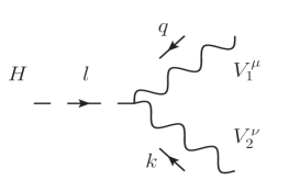
Figure 1: Illustration of the momenta in the $HVV$ interactions in Eq. (10).

The three momenta in the $HVV$ vertices in (10) are illustrated in FIG. 1, in which $l$ stands for the momentum of $H$, $q$ and $k$ stand for the momenta of the two gauge fields $V_{1}^{\mu}$ and $V_{2}^{\nu}$, respectively. They satisfy

$$l_{\mu}+q_{\mu}+k_{\mu}=0.$$ (12)

(a) The $H\gamma\gamma$ Interactions

$$g_{H\gamma\gamma}HA_{\mu\nu}A^{\mu\nu} \to 2g_{H\gamma\gamma}(q_{\nu}k_{\mu}-g_{\mu\nu}q\cdot k)A^{\mu}A^{\nu}H$$ (13)

$$= -2gM_{W}\rho_{H}\frac{s^{2}(f_{BB}+f_{WW})}{2\Lambda^{2}}$$

$$\times(q_{\nu}k_{\mu}-g_{\mu\nu}q\cdot k)A^{\mu}A^{\nu}H$$

(b) The $HZ\gamma$ Interactions

Taking $V_{1}^{\mu}=A^{\mu},V_{2}^{\mu}=Z^{\mu}$, we have

$$g_{HZ\gamma}^{(1)}A_{\mu\nu}Z^{\mu}\partial^{\nu}H+g_{HZ\gamma}^{(2)}HA_{\mu\nu}Z^{\mu\nu}$$

$$\to\bigg{[}g_{HZ\gamma}^{(1)}(q_{\mu}q_{\nu}-q^{2}g_{\mu\nu}+q_{\nu}k_{\mu}-g_{\mu\nu}q\cdot k)$$

$$+2g_{HZ\gamma}^{(2)}(q_{\nu}k_{\mu}-g_{\mu\nu}q\cdot k)\bigg{]}A^{\mu}Z^{\nu}H$$

$$=\frac{gM_{W}\rho_{H}s}{2c\Lambda^{2}}\bigg{[}(f_{W}-f_{B})(q_{\mu}q_{\nu}-q^{2}g_{\mu\nu})+\bigg{(}f_{W}-f_{B}$$

$$+4(s^{2}f_{BB}-c^{2}f_{WW})\bigg{)}(q_{\nu}k_{\mu}-g_{\mu\nu}q\cdot k)\bigg{]}A^{\mu}Z^{\nu}H$$ (14)

Neglecting the small term proportional to ${s}^{2}$, we have

$$g_{HZ\gamma}^{(1)}A_{\mu\nu}Z^{\mu}\partial^{\nu}H+g_{HZ\gamma}^{(2)}HA_{\mu\nu}Z^{\mu\nu}$$

$$\approx\frac{gM_{W}\rho_{H}s}{2c\Lambda^{2}}\bigg{[}(f_{W}-f_{B})(q_{\mu}q_{\nu}-q^{2}g_{\mu\nu})$$

$$+\bigg{(}f_{W}-f_{B}-4f_{WW}\bigg{)}(q_{\nu}k_{\mu}-g_{\mu\nu}q\cdot k)\bigg{]}A^{\mu}Z^{\nu}H.$$ (15)

(c) The $HWW$ Interactions

$$g_{HWW}^{(1)}(W^{+}_{\mu\nu}W^{-\mu}\partial^{\nu}H+{\rm h.c.})+g_{HWW}^{(2)}HW^{+}_{\mu\nu}W^{-\mu\nu}$$

$$~{}~{}\to\bigg{[}g_{HWW}^{(1)}(q_{\mu}q_{\nu}-q^{2}g_{\mu\nu}+k_{\mu}k_{\nu}-k^{2}g_{\mu\nu})$$

$$~{}~{}+2(g_{HWW}^{(1)}+g_{HWW}^{(2)})(q_{\nu}k_{\mu}-q\cdot kg_{\mu\nu})\bigg{]}W^{+\mu}W^{-\nu}H$$

$$~{}~{}=\frac{gM_{W}\rho_{H}}{2\Lambda^{2}}\bigg{[}f_{W}(q_{\mu}q_{\nu}-q^{2}g_{\mu\nu}+k_{\mu}k_{\nu}-k^{2}g_{\mu\nu})$$

$$~{}~{}+2(f_{W}-2f_{WW})(q_{\nu}k_{\mu}-q\cdot kg_{\mu\nu})\bigg{]}W^{+\mu}W^{-\nu}H$$ (16)

(d) The $HZZ$ Interactions

$$g_{HZZ}^{(1)}Z_{\mu\nu}Z^{\mu}\partial^{\nu}H+g_{HZZ}^{(2)}HZ_{\mu\nu}Z^{\mu\nu}$$

$$\to\bigg{[}\frac{1}{2}g_{HZZ}^{(1)}(q_{\mu}q_{\nu}-q^{2}g_{\mu\nu}+k_{\mu}k_{\nu}-k^{2}g_{\mu\nu})$$

$$+(g_{HZZ}^{(1)}+2g_{HZZ}^{(2)})(q_{\nu}k_{\mu}-g_{\mu\nu}q\cdot k)\bigg{]}Z^{\mu}Z^{\nu}H$$

$$=\frac{gM_{W}\rho_{H}}{2c^{2}\Lambda^{2}}\bigg{[}\frac{1}{2}(c^{2}f_{W}+s^{2}f_{B})$$

$$\times(q_{\mu}q_{\nu}-q^{2}g_{\mu\nu}+k_{\mu}k_{\nu}-k^{2}g_{\mu\nu})$$

$$+(c^{2}f_{W}+s^{2}f_{B}-2s^{4}f_{BB}-2c^{4}f_{WW})$$

$$\times(q_{\nu}k_{\mu}-g_{\mu\nu}q\cdot k)\bigg{]}Z^{\mu}Z^{\nu}H$$ (17)

Neglecting the small terms proportional to ${s}^{2}$ and ${s}^{4}$, we have

$$g_{HZZ}^{(1)}Z_{\mu\nu}Z^{\mu}\partial^{\nu}H+g_{HZZ}^{(2)}HZ_{\mu\nu}Z^{\mu\nu}$$

$$\approx\frac{gM_{W}\rho_{H}}{2c^{2}\Lambda^{2}}\bigg{[}\frac{1}{2}f_{W}(q_{\mu}q_{\nu}-q^{2}g_{\mu\nu}+k_{\mu}k_{\nu}-k^{2}g_{\mu\nu})$$

$$+(f_{W}-2f_{WW})(q_{\nu}k_{\mu}-g_{\mu\nu}q\cdot k)\bigg{]}Z^{\mu}Z^{\nu}H.$$ (18)

Now the gauge boson masses, especially the $W$ boson mass, are also contributed by more than one Higgs fields. Since ${\cal L}^{(6)}_{HVV}$ contains extra derivatives, it does not contribute to the $W$ boson mass. From (II.2) and (II.2) we see that

$$M_{W}^{2} = \frac{1}{4}(g_{h}^{2}v_{h}^{2}+g_{H}^{2}v_{H}^{2}+\cdots\cdots)$$ (19)

$$= \frac{1}{4}g^{2}v(\rho_{h}v_{h}+\rho_{H}v_{H}+\cdots\cdots).$$

Comparing with the SM $W$ boson mass $M_{W}^{2}=g^{2}v^{2}/4$, we obtain

$$\rho_{h}\frac{v_{h}}{v}+\rho_{H}\frac{v_{H}}{v}+\cdots\cdots=1.$$ (20)

This serves as another constraint on the gauge coupling constants and VEVs. It is easy to see that the two constraints (20) and (4) can be satisfied simultaneously.

III Unitarity Constraints on the Anomalous Coupling Constants

As we mentioned in the last section, the anomalous interactions in ${\cal L}^{(4)}_{HVV}+{\cal L}^{(6)}_{HVV}$ include five unknown anomalous coupling constants $\rho_{H},f_{W},f_{WW},f_{B},$ and $f_{BB}$. Low energy observables are insensitive to the related operators in ${\cal L}^{(6)}_{HVV}$. We are going to study certain constraints from high energy processes. In this section, we study the theoretical constraint obtained from the requirement of the unitarity of the $S$-matrix. In the next section, we shall study the experimental constraint obtained from the CMS $95\%$ CL exclusion bound on the SM Higgs boson.

We would like to emphasize that we are not aiming at precision calculations in this and the next sections. Instead, our purpose is to find out a rough range of the anomalous coupling constants $f_{W}$ and $f_{WW}$ with $f_{W}$ and $f_{WW}$ inside which the heavy Higgs boson is not excluded by the existing theoretical and experimental constraints, so that the study of probing the heavy Higgs boson at 14 TeV LHC makes sense.

Since the operators in ${\cal L}^{(6)}_{HVV}$ are momentum dependent, it will violate the unitarity of the $S$-matrix at high energies (note that the CM energy can not exceed $\Lambda$ in the effective Lagrangian theory). So that the requirement of the unitarity of the $S$-matrix can give constraints on the size of the anomalous coupling constants. This kind of study has been given in several papers unitarity in which the effective couplings for the single-Higgs system was taken, and the study is a single-parameter analysis. We cannot simply take such constraint in our study because we are studying the effective couplings in a multi-Higgs system taking account of the contributions of both the lightest SM-like Higgs $h$ and a heavier neutral Higgs boson $H$ with $\rho_{h},\rho_{H}\neq 1$. In the following, to get the order of magnitude constraints, we study the unitarity constraints for our case in the effective $W$ approximation (EWA).

The strongest constraints come from the longitudinal weak-boson scattering since the polarization vector $\epsilon_{L}^{\mu}$ of $W_{L}$ ($Z_{L}$) contains extra momentum dependence. To the precision of EWA, it is reasonable to neglect the small terms of $O(s^{2})$ and $O(s^{4})$ in the anomalous $HZZ$ coupling as in the last step in Eq. (18). Then we see from (16) and (18) that the relevant anomalous $HWW$ and $HZZ$ couplings contain only three unknown coupling constants $\rho_{H}$, $f_{W}$ and $f_{WW}$, irrelevant to $f_{B}$ and $f_{BB}$.

Expressing the $S$-matrix by $S=1-iT$, the unitarity of the $S$-matrix reads

$$|S^{\dagger}S|=|1-iT|^{2}=1$$ (21)

which leads to the following requirement

$$({\rm Re}\langle a|T|a\rangle)^{2}+({\rm Im}\langle a|T|a\rangle-1)^{2}+\sum_{|b\rangle\neq|a\rangle}\left|\langle b|T|a\rangle\right|^{2}=1$$

$$\Longrightarrow({\rm Re}\langle a|T|a\rangle)^{2}+\sum_{|b\rangle\neq|a\rangle}\left|\langle b|T|a\rangle\right|^{2}\leq 1.$$ (22)

When we take $|a\rangle=|W_{L}W_{L}\rangle$, the leading final state $\langle b|$ is $\langle W_{L}W_{L}|$ and $\langle Z_{L}Z_{L}|$. In certain regions of the anomalous coupling constants, the leading matrix element may be small, so that other non-leading final states should also be considered. Thus we also include $\langle b|=\langle W_{T}W_{T}|$, and $\langle Z_{T}Z_{T}|$. Similarly, when we take $|a\rangle=|Z_{L}Z_{L}\rangle$, we take $\langle b|=\langle Z_{L}Z_{L}|,\,\langle W_{T}W_{T}|$, and $\langle Z_{T}Z_{T}|$.

As usual, the unitarity constraints is to be calculated in the partial wave expression which was studied in detail in Ref. JW . It is well-known that the $S$-wave contribution is dominant. So we only calculate the matrix elements of the $S$-wave amplitude $T^{0}$. For $|a\rangle=|W_{L}W_{L}\rangle$ and $|a\rangle=|Z_{L}Z_{L}\rangle$, the unitarity constraints read

$$|{\rm Re}\langle W_{L}^{+}W_{L}^{-}|T^{0}|W_{L}^{+}W_{L}^{-}\rangle|^{2}+|\langle Z_{L}Z_{L}|T^{0}|W_{L}^{+}W_{L}^{-}\rangle|^{2}$$

$$+2|\langle W_{+}^{+}W_{+}^{-}|T^{0}|W_{L}^{+}W_{L}^{-}\rangle|^{2}+2|\langle Z_{+}Z_{+}|T^{0}|W_{L}^{+}W_{L}^{-}\rangle|^{2}$$

$$\leq 1,$$ (23)

and

$$|{\rm Re}\langle Z_{L}Z_{L}|T^{0}|Z_{L}Z_{L}\rangle|^{2}+2|\langle Z_{\pm}Z_{\pm}|T^{0}|Z_{L}Z_{L}\rangle|^{2}$$

$$~{}~{}+|\langle W_{L}^{+}W_{L}^{-}|T^{0}|Z_{L}Z_{L}\rangle|^{2}+2|\langle W_{\pm}^{+}W_{\pm}^{-}|T^{0}|Z_{L}Z_{L}\rangle|^{2}$$

$$~{}~{}\leq 1.$$ (24)

In our study, we have taken into account the contributions of both $h$ and $H$. These kinds of results have not been given in the published papers. We shall present our analytical results and numerical analysis as follows. We give the results in the center-of-mass (c.m.) frame, and express the scattering amplitudes in terms of the s,t,u parameters.

III.1 $W_{L}^{+}W_{L}^{-}\rightarrow VV$

$${\rm Re}\langle W_{L}^{+}W_{L}^{-}|T^{0}|W_{L}^{+}W_{L}^{-}\rangle=-\frac{g^{2}}{64\pi}\left\{\left[\rho_{H}^{2}(1-\frac{M_{W}^{2}}{\Lambda^{2}}f_{W})^{2}+\rho_{h}^{2}-1\right]\frac{{\sf s}}{M_{W}^{2}}+O({\sf s}^{0})\right\}.~{}~{}~{}~{}~{}~{}~{}~{}$$ (25)

$$\langle Z_{L}Z_{L}|T^{0}|W_{L}^{+}W_{L}^{-}\rangle=\frac{g^{2}}{32\pi}\bigg{\{}\bigg{[}\rho_{H}^{2}\bigg{(}1-\frac{M_{W}^{2}}{\Lambda^{2}}f_{W}\bigg{)}\bigg{(}\frac{M_{Z}^{2}}{\Lambda^{2}}f_{W}-1\bigg{)}-\rho_{h}^{2}+1\bigg{]}\frac{{\sf s}}{M_{W}^{2}}+O({\sf s}^{0})\bigg{\}}.$$ (26)

$$\langle W_{\pm}^{+}W_{\pm}^{-}|T^{0}|W_{L}^{+}W_{L}^{-}\rangle=\frac{\rho_{H}^{2}g^{2}}{32\pi}\bigg{(}1-\frac{M_{W}^{2}}{\Lambda^{2}}f_{W}\bigg{)}(2f_{WW}-f_{W})\frac{{\sf s}}{\Lambda^{2}}+O({\sf s}^{0}).$$ (27)

$$\langle Z_{\pm}Z_{\pm}|T^{0}|W_{L}^{+}W_{L}^{-}\rangle = \displaystyle\frac{\rho_{H}^{2}g^{2}}{32\pi}\bigg{(}1-\frac{M_{W}^{2}}{\Lambda^{2}}f_{W}\bigg{)}(2f_{WW}-f_{W})\frac{{\sf s}}{\Lambda^{2}}+O({\sf s}^{0}).$$ (28)

In (25)–(28), the terms with $\rho_{H}$ are the contributions of $H$, and those with $\rho_{h}$ are contributions of $h$. We see from (27) and (28) that, in these two matrix elements, the leading terms contain only the contributions of $H$ (from its dim-6 couplings).

III.2 $Z_{L}Z_{L}\to VV$

Since there are all ${\sf s},{\sf t}$ and ${\sf u}$ channel contributions in $Z_{L}Z_{L}\to Z_{L}Z_{L}$, the leading $O({\sf s}^{1})$ terms in the three channels just cancel with each other. So that

$${\rm Re}\langle Z_{L}Z_{L}|T^{0}|Z_{L}Z_{L}\rangle=O({\sf s}^{0}).$$ (29)

Results of other final states are

$$\langle Z_{\pm}Z_{\pm}|T^{0}|Z_{L}Z_{L}\rangle=\frac{\rho_{H}^{2}g^{2}}{32\pi}\bigg{\{}\left(1-\frac{M_{Z}^{2}}{\Lambda^{2}}f_{W}\right)(2f_{WW}-f_{W})\frac{{\sf s}}{\Lambda^{2}}+O({\sf s}^{0})\bigg{\}},$$ (30)

and

$$\langle W_{\pm}^{+}W_{\pm}^{-}|T^{0}|Z_{L}Z_{L}\rangle=\frac{\rho_{H}^{2}g^{2}}{32\pi}\bigg{\{}(2f_{WW}-f_{W})\left(1-\frac{M_{Z}^{2}}{\Lambda^{2}}f_{W}\right)\frac{{\sf s}}{\Lambda^{2}}+O({\sf s}^{0})\bigg{\}}.$$ (31)

We se that in (29)–(31), all the leading terms contain only the contributions of $H$ (from its dim-6 couplings).

With all the above results, we are ready to analyze the unitarity constraints on the anomalous coupling constants $f_{W}$ and $f_{WW}$. Since we are interested in weak-boson scattering at high energies in which ${\cal L}^{(6)}_{HVV}$ is enhanced, we shall only keep the terms with leading power of ${\sf s}$ in all the above results. In our numerical analysis, we simply take the s parameter to be its highest value ${\sf s}=\Lambda^{2}$. We shall study such constraints numerically performing a two-parameter analysis. Before doing that, we need to specify the other unknown parameters. First of all, as we have mentioned in Sec. II, we shall take $\Lambda=3$ TeV as an example. For $\rho_{h}$, the known SM-like properties of $h$ means that $\rho_{h}$ should not be so different from 1. We shall take $\rho_{h}=0.8,\,0.9$ as two examples. For $\rho_{H}$, we shall see in the next section that if $\rho_{H}>0.6$, the heavy neutral Higgs boson $H$ can hardly avoid being excluded by the CMS $95\%$ CL exclusion bounds on the SM Higgs boson. Therefore, for an existing $H$, $\rho_{H}$ should be less than 0.6. We shall take $\rho_{H}=0.6,\,0.4$ as two examples. The results of our analysis are shown in FIG. 2 in which FIG. 2(a) is with $\rho_{h}=0.8$, $\rho_{H}=0.6$, and FIG. 2(b) is with $\rho_{h}=0.9$, $\rho_{H}=0.4$. In FIG. 2, the red and blue-dashed contours are boundaries of the allowed regions obtained from $W_{L}^{+}W_{L}^{-}\to VV$ [Eq. (23)] and $Z_{L}Z_{L}\to VV$ [Eq. (24)], respectively.

We see that $\rho_{H}f_{W}/\Lambda^{2}$ and $\rho_{H}f_{WW}/\Lambda^{2}$ are constrained up to a few tens of TeV^-2 which is different from the results given in Ref. unitarity .

So far we have not concerned the unitarity bounds on $f_{B}$ and $f_{BB}$. In principle, they can be obtained by studying the scattering processes $W_{L}W_{L}\to\gamma\gamma$ and $W_{L}W_{L}\to Z\gamma$. However, since the photon has only transverse polarizations, such bounds will be weaker. Actually, in the next section, we shall argue that we may make the approximation of neglecting the anomalous coupling constants in the dim-6 couplings of the $H\gamma\gamma$ and $HZ\gamma$ couplings.

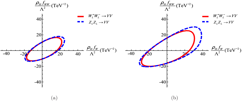
Figure 2: Unitarity bounds on $f_{W}$ and $f_{WW}$ in which (a) is with $\rho_{h}=0.8$ and $\rho_{H}=0.6$; (b) is with $\rho_{h}=0.9$ and $\rho_{H}=0.4$. The red and blue-dashed contours are boundaries of the allowed regions obtained from $W_{L}^{+}W_{L}^{-}\to VV$ [Eq. (23)] and $Z_{L}Z_{L}\to VV$ [Eq. (24)], respectively.

IV Experimental Constraints on Anomalous Coupling Constants

After the discovery of the 125–126 GeV Higgs boson in 2012, the CMS (ATLAS) Collaboration has made a lot of measurements on excluding the SM Higgs boson with mass up to 1 TeV (600 GeV) CMS_HIG_13_002 ATLAS_CMS12 others at $95\%$ C.L. For a NS heavy neutral Higgs boson, it must have large enough anomalous couplings to reduce its production cross section to avoid being excluded by the CMS experiments. This provides the possibility of constraining the anomalous coupling constants experimentally. In this section, we study such experimental bounds. Values of the anomalous coupling constants consistent with both the unitarity constraint and the experimental constraint are the available anomalous coupling constants that an existing heavy neutral Higgs boson can have.

Unlike what we did in the last section, we take account here the Higgs decay rates and the Higgs width to full leading order in perturbation, and we keep the nonvanishing weinberg angle, i.e., we use (14) and (17) rather than (15) and (18) for ${\cal L}^{(6)}_{HZ\gamma}$ and ${\cal L}^{(6)}_{HZZ}$. In our numerical analysis, we take FeynRules 2.0 FeynRules2.0 in our analysis code, and we use MADGRAPH5 MADGRAPH5 to calculate the Higgs production and decay rates.

In our effective couplings, there are altogether seven unknown parameters, namely $C_{t},\rho_{h},\rho_{H},f_{W},f_{WW},f_{B}$ and $f_{BB}$. So the analysis is rather complicated. From Eq. (11), we see that $f_{B}$ and $f_{BB}$ do not appear in the $HWW$ vertex, and they appear in the $HZZ$ vertex with the suppression factors $s^{2}$ and $s^{4}$, respectively. So their contributions to $VV$ scattering and $pp\to VH^{\ast}\to VVV$ studied in our next paper are negligibly small. They are mainly related to the decays $H\to\gamma\gamma$ and $H\to Z\gamma$. However, for the heavy Higgs boson with $M_{H}\geq 400$ GeV in our study, all the decay channels $H\to WW,H\to ZZ$ and $H\to t\bar{t}$ are open, so that the two decay channels $H\to\gamma\gamma$ and $H\to Z\gamma$ are relatively not so important. Since we are not aiming at doing precision calculations, we may take certain approximation to avoid dealing with $f_{B}$ and $f_{BB}$ in the analysis to simplify it.

We then examine the ATLAS and CMS results of the strength $\mu=\left.\sigma/\sigma_{SM}\right|_{95\%~{}CL}$ for the decay channels $H\to\gamma\gamma$ ATLAS_PRL12 CMS_PAS_HIG_13_001 and $H\to Z\gamma$ ATLAS_1402.3051 CMS_1307.5515 . Unfortunately, the data only exist below 150 GeV which does not include the range $M_{H}\geq 400$ GeV in our study. So we can only make a speculation of the situation in the range above 150 GeV. We see from the results in Refs. ATLAS_PRL12 CMS_PAS_HIG_13_001 ATLAS_1402.3051 CMS_1307.5515 that the trend of the ATLAS and CMS results below 150 GeV is that the experimental curves tend to gradually go closer to the $\mu=1$ axis. So we roughly estimate that they may keep this situation above 150 GeV. This means that there is no evidence of needing significant anomalous couplings in the $H\gamma\gamma$ and $HZ\gamma$ couplings, i.e., we just neglect the anomalous coupling constants of the effective $H\gamma\gamma$ and $HZ\gamma$ interactions. We frist see from Eq. (13) that neglecting the anomalous coupling constant in Eq. (13) means

$$f_{BB}\approx-f_{WW}.$$ (32)

We then see from Eq. (14) that there are two terms in it. The first term is proportional to $(q_{\mu}q_{\nu}-q^{2}g_{\mu\nu})A^{\mu}$ which vanishes for on-shell photon. Thus neglecting the anomalous coupling constant in Eq. (14) means

$$f_{B}\approx f_{W}-4f_{WW}.$$ (33)

Eqs. (32) and (33) serve as two constraints on $f_{BB}$ and $f_{B}$, expressing them in terms of $f_{W}$ and $f_{WW}$. Then we have only five unknown coupling constants left, namely $C_{t},\,\rho_{h},\,\rho_{H},\,f_{W}$ and $f_{WW}$, as in the last section.

Next we look at ${\cal L}^{(6)}_{HWW}$ and ${\cal L}^{(6)}_{HZZ}$. We see from (16) that ${\cal L}^{(6)}_{HWW}$ does not contain $f_{B}$ and $f_{BB}$, so it is unaffected by the approximations (32) and (33). However, ${\cal L}^{(6)}_{HZZ}$ does contain $f_{B}$ and $f_{BB}$. With the approximations (32) and (33), Eq. (17) becomes

$${\cal L}^{(6)}_{HZZ}=\frac{gM_{W}\rho_{H}}{2c^{2}\Lambda^{2}}\bigg{[}\frac{1}{2}(f_{W}-4s^{2}f_{WW})$$

$$\times(q_{\mu}q_{\nu}-q^{2}g_{\mu\nu}+k_{\mu}k_{\nu}-k^{2}g_{\mu\nu})$$

$$+(f_{W}-2f_{WW})(q_{\nu}k_{\mu}-g_{\mu\nu}q\cdot k)\bigg{]}Z^{\mu}Z^{\nu}H.$$ (34)

Now we consider the CMS and ATLAS exclusion bounds on SM Higgs boson CMS_HIG_13_002 ATLAS_CMS12 others . The strongest one is CMS result obtained from the $H\to ZZ\to 4\ell$ channel CMS_HIG_13_002 . In this section, we mainly consider this strongest bound, and we also take account of other weaker bounds others when considering the size of the available range for $f_{W}$ and $f_{WW}$.

The strongest CMS exclusion bound is given in the Higgs mass range up to 1 TeV. Its feature is that the experimental curve goes rapidly away from the $\mu=1$ axis (below $\mu=1$) above 120 GeV, and fluctuates in the range between 140 GeV and 400 GeV, and then goes relatively smoother towards the $\mu=1$ axis up to 1 TeV. In view of the significant fluctuations below 400 GeV, we shall take $M_{H}$=400 GeV, 500 GeV and 800 GeV as examples to do the two-parameter analysis. The parameters in these examples are:

i, 400II: $M_{H}=400$ GeV, $C_{t}=0.5$ (Type-II),
     $\rho_{h}=0.9$, $\rho_{H}=0.4$,
ii, 500I: $M_{H}=500$ GeV, $C_{t}=1$ (Type-I), $\rho_{h}=0.9$,
     $\rho_{H}=0.4$,
iii, 500II: $M_{H}=500$ GeV, $C_{t}=0.6$ (Type-II), $\rho_{h}=0.8$,
     $\rho_{H}=0.6$,
iv, 800I: $M_{H}=800$ GeV, $C_{t}=1$ (Type-I), $\rho_{h}=0.8$,
     $\rho_{H}=0.6$,
v, 800II: $M_{H}=800$ GeV, $C_{t}=0.2$ (Type-II), $\rho_{h}=0.9$,
     $\rho_{H}=0.25$,

When calculating the strength $\mu$ for $H\to ZZ\to 4\ell$, we need to calculate

$$\sigma=\sigma(pp\to HX)B(H\to ZZ\to 4\ell),$$

$$B(H\!\to\!ZZ\!\to\!4\ell)=\frac{\Gamma(H\!\to\!ZZ\!\to\!4\ell)}{\Gamma(H\!\to\!ZZ)+\Gamma(H\!\to\!WW)+\cdots}.~{}~{}~{}~{}$$ (35)

The total decay width $\Gamma(H\!\to\!ZZ)+\Gamma(H\!\to\!WW)+\cdots$ needs further discussion. Apart from the decay modes related to the effective coupling mentioned in Sec. II, there can also be the decay mode $H\to hh$ caused by an effective coupling $\lambda v_{H}Hhh$ (note that $H$ is the lightest heavy Higgs boson so that it can not decay to other heavy Higgs bosons). For $H$ with $M_{H}\geq 400$ GeV, all the decay channels $H\to WW,\,H\to ZZ$ and $H\to t\bar{t}$ are open. Since $M_{h}$ is larger than $M_{W}$ and $M_{Z}$, the phase space in $H\to hh$ is smaller than those in $H\to WW$ and $H\to ZZ$. Thus the mode $H\to hh$ does not play an important role in the total width. Since we are not aiming at doing precision calculations, we can make the approximation of neglecting the $H\to hh$ mode in the total decay width of $H$ to avoid introducing a new unknown parameter $\lambda$. In this approximation, our obtained total decay width of $H$ is smaller than its actual value. This makes the obtained exclusion constraint on $H$ stronger than what it actually is. Thus our approximate calculation is a conservative calculation, i.e., the required values of $f_{W}$ and $f_{WW}$ from our approximate exclusion bound are more than enough for avoiding being excluded by the actual exclusion bound. This guarantees that a heavy Higgs boson $H$ with the obtained allowed values of $f_{W}$ and $f_{WW}$ is definitely not excluded by the CMS exclusion bound CMS_HIG_13_002 .

Now we present our two-parameter numerical analysis results.

1. $M_{H}=$400 GeV

As we have mentioned, the exclusion bound is very strong at $M_{H}=400$ GeV. Our numerical analysis shows that, for the case of Type-I, a NS heavy neutral Higgs boson with $M_{H}=400$ GeV can hardly avoid being excluded. Of course, if we take $\rho_{H}$ to be small enough, it may help. But a heavy neutral Higgs boson with so small gauge interactions is not considered in this study, and will be considered elsewhere.

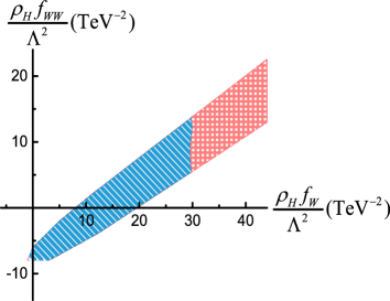
Figure 3: Obtained experimental bound on $f_{W}$ and $f_{WW}$ in the case of 400II. The blue shaded region is the available region.

Now we consider case of 400II. The small $C_{t}$ reduces the Higgs production cross section by gluon fusion $\sigma(pp\to HX)$, so that the requirement of reducing $B(H\to ZZ\to 4\ell)$ is milder, and it is possible to find out the available values of $f_{W}$ and $f_{WW}$. The result of our two-parameter numerical analysis is shown in FIG. 3. The shaded region means the values of $f_{W}$ and $f_{WW}$ which can sufficiently reduce the branching ratio $B(H\to ZZ\to 4\ell)$ such that the heavy neutral Higgs boson is not excluded by the CMS exclusion bound. Considering further the unitarity bound in FIG. 2(b), we find that the real available region (consistent with the unitarity bound) is the part shaded in blue.

2. $M_{H}$=500 GeV

For $M_{H}=500$ GeV, the SM Higgs exclusion bound is looser. We take two sets of parameters as examples, namely 500I (Type-I) case with $C_{t}=1,\,\rho_{h}=0.9,\,\rho_{H}=0.4$; and 500II (Type-II) case with $C_{t}=0.6,\,\rho_{h}=0.8,\,\rho_{H}=0.6$.

We first look at the 500I case. The result of our two-parameter numerical analysis is shown in FIG. 4 in which the shaded region is the region of $f_{W}$ and $f_{WW}$ making the heavy neutral Higgs boson $H$ not excluded by the CMS exclusion bound, and the small part shaded in blue is consistent with the unitarity bound shown in FIG. 2(b), i.e., the available region. Note that this is also in the first quadrant of the $f_{W}$-$f_{WW}$ plane.

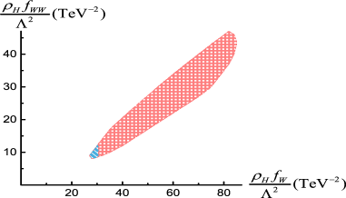
Figure 4: Obtained experimental bound on $f_{W}$ and $f_{WW}$ in the case of 500I. The blue shaded region is the available region.

Next we look at the 500II case. The result of our two-parameter numerical analysis is shown in FIG. 5 in which the blue shade region is the available region (the whole region is consistent with the unitarity bound shown in FIG. 2(a)). These available region is in the third and fourth quadrants. Since the value $\rho_{H}=0.6$ is larger than that in the 500I case, the needed values of $f_{W}$ and $f_{WW}$ for sufficiently reducing $B(H\to ZZ\to 4\ell)$ in the first quadrant are so large that they exceed the unitarity bound shown in FIG. 2(a). Thus only the region shown in FIG. 5 is really available.

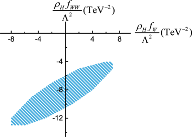
Figure 5: Obtained experimental bound on $f_{W}$ and $f_{WW}$ in the case of 500II. The blue shaded region is the available region.

3. $M_{H}$=800 GeV

We see from the CMS exclusion bound CMS_HIG_13_002 that the exclusion bound at $M_{H}$=800 GeV is very loose, so that almost all values of $f_{W}$ and $f_{WW}$ are available to make the heavy neutral Higgs boson not excluded by the CMS exclusion bound. In the 800I case, $C_{t}=1$, the total decay width of the 800 GeV heavy neutral Higgs boson is quite large that it is not possible to see a resonance bump at the LHC, but it is still possible to detect it by measuring the cross section. In the 800II case, a sufficiently small value of $C_{t}$ will make the total decay width small enough that a resonance bump can be seen at the LHC.

To understand why the available regions in FIGs. 3, 4 and 5 are so different, let us look at how $f_{W}$ and $f_{WW}$ affect $\Gamma(H\to WW)$ and $\Gamma(H\to ZZ)$. Below are our obtained results of $\Gamma(H\to WW)$ and $\Gamma(H\to ZZ)$.

$$\Gamma(H\to WW)\approx\frac{g^{2}\rho_{H}^{2}M_{H}^{3}}{64\pi M_{W}^{2}}\left[\left(1-\frac{M_{W}^{2}}{\Lambda^{2}}f_{W}\right)^{2}\right.$$

$$~{}~{}\left.+2\frac{M_{W}^{4}}{\Lambda^{4}}(f_{W}-2f_{WW})^{2}+O\left(\frac{M_{W}^{2}}{M_{H}^{2}}\right)\right],$$ (36)

$$\Gamma(H\to ZZ)\approx\frac{g^{2}\rho_{H}^{2}M_{H}^{3}}{128\pi M_{W}^{2}}\left[\left(1\!-\!\frac{M_{Z}^{2}}{\Lambda^{2}}(f_{W}\!-\!4s^{2}f_{WW})\right)^{2}\right.$$

$$~{}~{}\left.+2\frac{M_{Z}^{4}}{\Lambda^{4}}(f_{W}-2f_{WW})^{2}+O\left(\frac{M_{W}^{2}}{M_{H}^{2}}\right)\right],$$ (37)

First of all, we see from (36) and (37) that, if $f_{W}$ and $f_{WW}$ are in the second quadrant of the $f_{W}$-$f_{WW}$ plane, i.e., $f_{W}<0,\,f_{WW}>0$, they always increase $\Gamma(H\to WW)$ and $\Gamma(H\to ZZ)$, and $\Gamma(H\to ZZ)$ is increased more than $\Gamma(H\to WW)$ is. In this case, $B(H\to ZZ\to 4\ell)$ is always increased, so that the heavy Higgs boson $H$ is definitely excluded by the CMS exclusion bound, i.e., there is no available region of $f_{W}$ and $f_{WW}$ in the second quadrant of the $f_{W}$-$f_{WW}$ plane. It is so in FIGs. 3, 4 and 5.

Next we look at the case that $\left|f_{W}\right|,\,\left|f_{WW}\right|<\Lambda^{2}/M_{W}^{2}$ with $f_{W}-2f_{WW}$ not too large. We see from (36) and (37) that, for $f_{W}$ and $f_{WW}$ in the first quadrant ($f_{W}>0,\,f_{WW}>0$), $\Gamma(H\to WW)$ and $\Gamma(H\to ZZ)$ are all decreased, and $\Gamma(H\to WW)$ is decreased more than $\Gamma(H\to ZZ)$ is. So that $B(H\to ZZ\to 4\ell)$ is increased, i.e., there is no available region of $f_{W}$ and $f_{WW}$ in the first quadrant of the $f_{W}$-$f_{WW}$ plane. However, in the third quadrant ($f_{W}<0,\,f_{WW}<0$) and the fourth quadrant ($f_{W}>0,\,f_{WW}<0$), either $\Gamma(H\to WW)$ is increased more than $\Gamma(H\to ZZ)$ is, or $\Gamma(H\to WW)$ is decreased less than $\Gamma(H\to ZZ)$ does. Thus in these two quadrants, $B(H\to ZZ\to 4\ell)$ is reduced, so that there can be available region of $f_{W}$ and $f_{WW}$ in the third and fourth quadrants of the $f_{W}$-$f_{WW}$ plane. This is just the situation in FIG. 5. In the special case of 400IIwith $C_{t}=0.5$ which significantly reduces the Higgs production cross section $\sigma(pp\to HX)$, in addition to the third and fourth quadrants, there can also be available region in the first quadrant even $B(H\to ZZ\to 4\ell)$ is increased a little there. Thus in this special case, there can be available regions in the first, third, and fourth quadrants. This is the situation in FIG. 3.

We then look at the case that $\left|f_{W}\right|,\,\left|f_{WW}\right|\sim\Lambda^{2}/M_{W}^{2}$. In this case, we should examine both the first and second terms in (36) and (37). In the first quadrant, the first terms are quite small, and the second terms (proportional to $f_{W}-2f_{WW}$) can also be small when $f_{W}\approx 2f_{WW}$, while the total decay rate [the denominator in Eq. (35)] is not reduced so much since $\Gamma(H\to t\bar{t})$ is not so small. So, in this case, $B(H\to ZZ\to 4\ell)$ can be sufficiently reduced. In the fourth quadrant, the second terms are not small enough, and in the third quadrant, the first terms are not small enough. So that in the third and fourth quadrants $B(H\to ZZ\to 4\ell)$ cannot be sufficiently reduced. Thus in this case there can be available region of $f_{W}$ and $f_{WW}$ only in the first quadrant of the $f_{W}$-$f_{WW}$ plane. This is the situation in FIG. 4.

When $\left|f_{W}\right|$ and $\left|f_{WW}\right|$ become larger and larger, the constant terms (independent of $f_{W}$ and $f_{WW}$) in (36) and (37) are less and less important. In this case, $\Gamma(H\to WW)$ and $\Gamma(H\to ZZ)$ all increase, and they are different only by the term containing $4s^{2}f_{WW}$. it can be shown that, in this case,

$$\Gamma(H\to ZZ)\nless 0.2\,\Gamma(H\to WW),$$ (38)

or

$$\frac{\Gamma(H\to ZZ)}{\Gamma(H\to WW)+\Gamma(H\to ZZ)}\nless 0.17.$$ (39)

Comparing the corresponding SM values, our detailed analysis shows that, for $M_{H}$= 400 GeV and 500 GeV, this is not small enough for sufficiently reducing $B(H\to ZZ\to 4\ell)$ to avoid being excluded by the CMS bound in Ref. CMS_HIG_13_002 . Thus the available values of $\left|f_{W}\right|$ and $\left|f_{WW}\right|$ cannot be arbitrarily large. This is why the available regions in FIG. 3, FIG. 4, and FIG. 5 are all closed regions.

Finally, we would like to add a discussion on whether it is reasonable to simply apply the CMS exclusion bound to our examples with new physics interactions as what we did above. We know that the detection efficiency of the detector depends on specific interactions, and the detection efficiency of the CMS exclusion bound in Ref. CMS_HIG_13_002 is for the SM interaction. We shall take 400II with $\rho_{H}f_{W}/\Lambda^{2}=30$ TeV^-2 and $\rho_{H}f_{WW}/\Lambda^{2}=10$ TeV^-2., 500I with $\rho_{H}f_{W}/\Lambda^{2}=30$ TeV^-2, and $\rho_{H}f_{WW}/\Lambda^{2}=10$ TeV^-2, and 500II with $\rho_{H}f_{W}/\Lambda^{2}=6$ TeV^-2 and $\rho_{H}f_{WW}/\Lambda^{2}=-5$ TeV^-2 as examples to calculate how much their detection efficiencies deviate from the that with the SM interaction.

We shall make a calculation to study how much such deviations actually are in detecting $pp\to H\to ZZ\to\ell^{+}\ell^{-}\ell^{+}\ell^{-}$ at the 8 TeV LHC. We use DELPHES 3 DELPHES3 to roughly simulate the detector. We use MADGRAPH 5 to do the simulation, and use MadAnalysis to obtain the efficiency.

In our calculation, we have chosen 60 GeV $<M(\ell^{+}\ell^{-})<$120 GeV to guarantee that the two final states $\ell^{+}$ and $\ell^{-}$ are from the decay of a $Z$ boson. We have also chosen 200 GeV$<M(\ell^{+}\ell^{-}\ell^{+}\ell^{-})<$ 600 GeV and 300 GeV$<M(\ell^{+}\ell^{-}\ell^{+}\ell^{-})<$ 700 GeV to guarantee the final state $\ell^{+}\ell^{-}\ell^{+}\ell^{-}$ are from the decay of our heavy Higgs bosons under consideration.

The obtained detection efficiency for detecting $H\to ZZ\to\ell^{+}\ell^{-}\ell^{+}\ell^{-}$ is listed in TABLE 1.

Table 1: Comparison of the detection efficiencies between the SM and our examples: 400II with $\rho_{H}f_{W}/\Lambda^{2}=30$ TeV^-2 and $\rho_{H}f_{WW}/\Lambda^{2}=10$ TeV^-2., 500I with $\rho_{H}f_{W}/\Lambda^{2}=30$ TeV^-2, and $\rho_{H}f_{WW}/\Lambda^{2}=10$ TeV^-2, and 500II with $\rho_{H}f_{W}/\Lambda^{2}=6$ TeV^-2 and $\rho_{H}f_{WW}/\Lambda^{2}=-5$ TeV^-2.

	400II	SM ($M_{H}=400$ GeV)	500I	500II	SM ($M_{H}=500$ GeV)
detection efficiency	$17.9\%$	$17.7\%$	$18.6\%$	$18.8\%$	$17.6\%$

We see that, for 400II, the new interaction causes a relative change of the efficiency with respect to the SM efficiency by $(17.9\%-17.6\%)/17.6\%=2\%$. For 500I and 500II, the corresponding relative changes of the efficiency are $(18.6\%-17.6\%)/17.6\%=6\%$ and $(18.8\%-17.6\%)/17.6\%=7\%$, respectively. Since we are not aiming at doing precision calculations, a few percent change will not affect our main conclusions in simply applying the CMS exclusion bound to our examples..

V General features of studying the LHC signatures of $\bm{H}$

For the study of the LHC signatures of $H$ at the 14 TeV LHC, we do not suggest taking the conventional on-shell Higgs production, used in studying the properties of the 125–126 GeV Higgs boson, to probe the anomalous heavy Higgs boson, The reason is the following. Comparing Eq. (10) with Eq. (II.2) in Sec. II, we see that the dim-6 interaction contains an extra factor $k^{2}/\Lambda^{2}$ relative to the dim-4 interaction, coming from the extra derivatives in Eq. (10). Here $k$ is a typical momentum of the order of the momentum of the Higgs boson. In on-shell Higgs production, $k^{2}\sim M_{H}^{2}$. Taking $M_{H}=500$ GeV as an example, $k^{2}/\Lambda^{2}\sim M_{H}^{2}/\Lambda^{2}=0.25/9=0.03$. Thus the contribution of the dim-6 interaction is only a very tiny portion of the total contribution, so that it is hard to detect the dim-6 interaction effect in on-shell Higgs production.

Instead, in this paper, we suggest taking $VV$ scattering and $pp\to VH^{\ast}\to VVV$ as sensitive processes for probing the anomalous heavy Higgs boson at the 14 TeV LHC. These processes contain off-shell heavy Higgs contributions. In the tail with energy higher than the resonance peak, $k^{2}/\Lambda^{2}$ can be larger. Although the tail with much higher energy than the resonance is seriously suppressed by the parton distribution (e.g., the region $k^{2}\lesssim\Lambda^{2}$ is almost completely suppressed), the remaining high energy tail can still enhance the contribution of the dim-6 interaction as we shall see in Secs. VI–VIII. Furthermore, each of these two processes contains two $HVV$ vertices. This makes the cross sections more sensitive to the anomalous couplings than in on-shell Higgs production.

Although the two suggested processes are weak-interaction processes with not so large cross sections, the signal to background ratio can be effectively improved by imposing a series of proper cuts. So that the integrated luminosity needed for $3\sigma$ and $5\sigma$ deviations are not so high (e.g., see TABLE 6) in Sec. VII.

That weak-boson scattering can be a sensitive process for detecting an anomalous Higgs boson at the LHC was first pointed out in Ref. ZKHY03 , in which the effective couplings for a single-Higgs system, and the pure leptonic decay mode of the final state $W$ bosons was considered. It showed that the required integrated luminosity was high. Ref. QKLZ09 studied the same problem but with the semileptonic decay channel (one of the final state $W$ boson decays to leptons and the other $W$ boson decays to jets), and showed that the required integrated luminosity was significantly reduced.

Thus we shall study the semileptonic decay mode in both the weak-boson scattering and $pp\to VH^{\ast}\to VVV$ processes, i.e., $pp\to VVj^{f}_{1}j^{f}_{2}\to\ell^{+}\nu_{\ell}j_{1}j_{2}j^{f}_{1}j^{f}_{2}$ ($j^{f}_{1},\,j^{f}_{2}$ stand for forward jets) in weak-boson scattering, and $pp\to VH^{\ast}\to VVW\to\ell^{+}\nu_{\ell}j_{1}j_{2}j_{3}j_{4}$ in the $pp\to VH^{\ast}\to VVV$ process. Since there are several jets in the final states, parton-level calculation is not adequate. We shall do the calculation to the hadron level.

We take the CTEQ6.1 parton distribution functions CTEQ6.1 , and use MADGRAPH5 MADGRAPH5 to do the full tree-level simulation. The parton shower and hadronization are calculated with PYTHIA6.4 PYTHIA6.4 , and the anti-$k_{T}$ algorithm antik_T in DELPHES 3 DELPHES3 is used for the formation of jets with $R=0.7$ CMS2011 . We also use DELPHES 3 to simulate the detecting efficiency of the detector. We take the five examples in Sec. IV to do the simulation, and take the acceptance of the detector listed in TABLE 2.

Table 2: The detector acceptance.

	$|\eta|_{max}$	$P_{T{\rm min}}$
$\mu$	2.4	10GeV
$e$	2.5	10GeV
jet	5	20GeV
photon	2.5	0.5GeV

In each process, we regard the contributions by the heavy Higgs boson $H$ as the signal, other contributions without $H$ as backgrounds. Among the backgrounds processes, the process with the same initial- and final-state is regarded as the irreducible background (IB), others are reducible backgrounds (RB). The signal and the IB should be calculated together since they have interference. Let $\sigma$ be the total cross section. The background and the signal cross sections are then defined as

$$\sigma_{B}=\sigma(C_{t}=1,\rho_{h}=1,\rho_{H}=0,f_{W}=0,f_{WW}=0),$$

$$\sigma_{S}=\sigma-\sigma_{B}.$$ (40)

For an integrated luminosity ${\sf L}_{int}$, The signal and background event numbers are $N_{S}={\sf L}_{int}\sigma_{S},\,\,N_{B}={\sf L}_{int}\sigma_{B}$. In this paper, we take the Poisson distribution approach to determine the statistical significance $\sigma_{stat}$. The general Poisson probability distribution reads

$$\displaystyle P_{B} = \sum_{N}\displaystyle e^{-N_{B}}\frac{N_{B}^{N}}{N!},$$ (41)

$$N=N_{S}+N_{B},N_{S}+N_{B}+1,\cdots,\infty.$$

Comparing the obtained value of $1-P_{B}$ with the probability of the signal in the Gaussian distribution, we can find out the corresponding value of $\sigma_{stat}$ PDG . The value of $\sigma_{stat}$ obtained in this way approaches to the simple form

$$\sigma_{stat}=\frac{N_{S}}{\sqrt{N}_{B}}$$ (42)

when $N_{S}$ and $N_{B}$ are sufficiently large.

VI Probing Heavy Neutral Higgs Bosons via Weak-Boson scattering

In this section, we study the semileptonic mode of weak-boson scattering, $pp\to VVj^{f}_{1}j^{f}_{2}\to\ell^{+}\nu_{\ell}j_{1}j_{2}j^{f}_{1}j^{f}_{2}$. We first look at the Feynman diagrams of the signal, IB, and RBs in this process. Feynman diagrams for the signal and examples of the IB are shown in FIG. 6

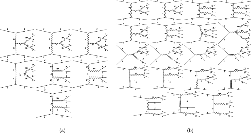
Figure 6: Feynman diagrams in weak-boson scattering. (a) the signal, (b) examples of the IB.

These two kinds of diagrams in FIG. 6(a) and FIG. 6(b) should be calculated together since they have interference.

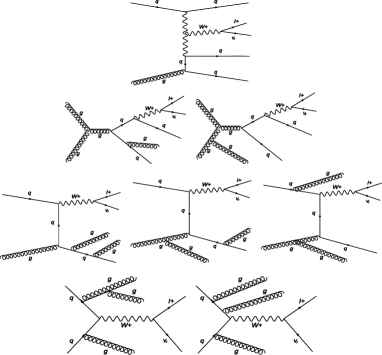
Figure 7: Feynman diagrams for QCD backgrounds of $W+3j$.

Apart from the IB, there are two kinds of RBs, namely the so-called QCD backgrounds and top-quark backgrounds Bagger9495 . Note that the two jets $j_{1}$ and $j_{2}$ from $W$ decay mainly behave as a “single” energetic fat jet $J$ along the $W$ direction Butterworth CMS_JME_13_006 since the final state $W$ is very energetic. This is the reason why we take $R=0.7$ in the anti-$k_{T}$ algorithm. In this case, the important QCD backgrounds which can mimic the signal at the hadron level are the the inclusive $W+3j$ (with $W\to\ell^{+}\nu_{\ell}$, and the three jets mimic the fat jet $J$ and the two forward jets) and the $WV+2j$ (with $W\to\ell^{+}\nu_{\ell}$, $V\to J$, and the two jets mimic the two forward jets). The parton-level Feynman diagrams of these two QCD backgrounds are shown in FIGs. 7 and FIGs. 8. These two QCD backgrounds have been discussed in Ref. QKLZ09 . In our calculation, we match the partons with jets using the method in Refs. MMP02 Aetal08 to obtain the inclusive $W+3j$ and inclusive $WV+2j$ backgrounds.

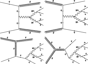
Figure 8: Feynman diagrams for QCD backgrounds of $WV+2j$.

The top-quark background is $pp\to t\bar{t}\to W^{+}bW^{-}\bar{b}\to\ell^{+}\nu_{\ell}j_{1}j_{2}b\bar{b}$ with $j_{1}j_{2}b\bar{b}$ mimicking the two jets in $W$ decay and the two forward jets. The Feynman diagrams of the top-quark background are shown in FIB. 9.

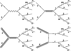
Figure 9: Feynman diagrams for the top-quark backgrounds.

We shall take the following kinematic cuts, reflecting the properties of the signal, to suppress the backgrounds and keep the signal as much as possible.

cut1: Requiring an isolated lepton $\ell^{+}\,(\mu^{+},\,e^{+})$ in the central rapidity region

$$N(\ell^{+})=1,~{}~{}~{}~{}N(\ell^{-})=0$$

$${\rm with}~{}~{}~{}~{}~{}~{}~{}~{}~{}~{}~{}~{}~{}~{} \left|\eta_{\ell^{+}}\right|<2.$$ (43)

Since the signal lepton has larger probability to be in the central rapidity region than the RBs do, this cut will suppress the RBs relative to the signal. Furthermore, there can be fake leptons ($\ell^{+}\,\,{\rm or}\,\,\ell^{-}$) coming from the decays of the hadrons $\pi,\,\eta,\,J/\psi$, etc. in the hadronized jets. This cut can also suppress the fake leptons.

cut2: $p_{T}(leptons)$-cut

Let ${\bm{p}}_{T}(\ell^{+})$ and  $/\!\!\!\!{\bm{p}}_{T}\equiv{\bm{p}}_{T}(\nu_{\ell})$ be the transverse momentum vectors of $\ell^{+}$ and $\nu_{\ell}$, respectively.

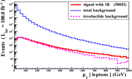
Figure 10: $p_{T}(leptons)$ distributions of signal+IB (red-solid), IB (pink-dotted) and total RBs (blue-small-dotted) in weak-boson scattering for the example 500II with ${\sf L}_{int}=$100 fb^-1.

Our simulation shows that a cut on $p_{T}(leptons)\equiv\left|{\bm{p}}_{T}(\ell^{+})+/\!\!\!\!{\bm{p}}_{T}\right|$ can effectively suppress both the IB and the RBs. FIG. 10 plots the inclusive $p_{T}(leptons)$ distributions of the signal plus IB (red-solid), the IB (pink-dotted), and the total RBs (blue-small-dotted) for example 500II with ${\sf L}_{int}=$100 fb^-1. We see from FIG. 10 that taking a cut

$$p_{T}(leptons)>150\,{\rm GeV}$$ (44)

can suppress both the IB and the total RBs, while keep the signal as much as possible. It can also suppress fake leptons very effectively since the scale of the transverse momenta of fake leptons is of the order of the hadronization scale which is much smaller than the required $p_{T}(leptons)$ in (44).

cut3: Forward-jet cuts

The signal has two clear forward jets $j^{f}_{1}$ and $j^{f}_{2}$ which characterize the weak-boson fusion process, while in some RBs, the jets which mimic $j^{f}_{1}$ and $j^{f}_{2}$ may not be forward. So that we can set cuts reflecting the properties of $j^{f}_{1}$ and $j^{f}_{2}$ to suppress the RBs. There have been several ways of setting the forward-jet cuts. We follow the way in Ref. Butterworth but with a little modification

$$p_{T}(j^{f})>35~{}{\rm GeV},$$

$$E(j^{f})>300~{}{\rm GeV},$$

$$2.0<|\eta(j^{f})|<5,~{}~{}~{}~{}~{}~{}\eta(j^{f}_{1})\eta(j^{f}_{2})<0.$$ (45)

In the cut for $|\eta(j^{f})|$, we have taken account of the acceptance of the detector (cf. TABLE 2). Here, instead of taking $p_{T}(j^{f})>20~{}{\rm GeV}$ as in Ref. Butterworth , we take $p_{T}(j^{f})>35~{}{\rm GeV}$ for avoiding the pileup events.

In our simulation, we take the jet with most positive $\eta$ and the jet with most negative $\eta$ to satisfy the rapidity requirement in (45).

cut4: Fat jet cuts

In the signal, the fat jet $J$ (the jet with largest transverse momentum) is the decay product of a $W$ boson, so that the invariant mass $M(J)$ of $J$ should equal to $M_{W}$. Considering the resolution of the detector, we set the requirement

$$70\,{\rm GeV}<M(J)<100\,{\rm GeV}.$$ (46)

This requirement can effectively suppress the largest reducible background $W+3j$ since, in $W+3j$, the largest $p_{T}$ ordinary jet $\hat{j}$ which mimics $J$ comes from the clustering of the parton showers from a massless parton. For most of the probability, its mass $M(\hat{j})$ is much smaller than the requirement (46).

Furthermore, in the signal, the fat jet $J$ and the isolate lepton $\ell^{+}$ are decay products of the two $W$ bosons in $H$ decay. With the cut (43), we also set

$$|\eta_{J}|<2$$ (47)

to suppress the backgrounds.

cut5: Top-quark veto

We see from FIG. 9 that, in a top-quark background event, $t\to W^{+}b\to\ell^{+}{\bar{\nu}}_{\ell}b$, $\bar{t}\to W^{-}{\bar{b}}\to J{\bar{b}}$. So that, to identify a top-quark background event, we can construct the invariant mass $M(J,\bar{b})$ to reconstruct the top quark. Experimentally, $M(J,\bar{b})$ must be in the top-quark resonance region around $m_{t}$. On the other hand, if we construct $M(J,b)$ it will not be in the top-quark resonance region. However, in the experiment, we can just see three jets $J,\,j_{1},\,j_{2}$ in the final state, and cannot identify which one of $j_{1}$ and $j_{2}$ is the $\bar{b}$ jet. So we should construct two invariant masses $M(J,j_{1})$ and $M(J,j_{2})$ to see if one of them is in the top-quark resonance region to identify whether an event is a top-quark background event. In FIG. 11 we plot the $M(J,j_{1})$ [or $M(J,j_{2})$] distribution from our simulation including the signal plus IB (red-solid) and the top-quark background (blue-dotted) distributions for the example 500II with ${\sf L}_{int}=$100 fb^-1.

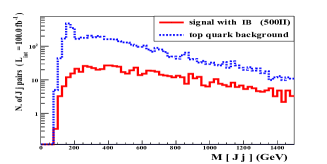
Figure 11: $M(J,j)$ distributions of signal+IB (red-solid) and the top-quark background (blue-dotted) in weak-boson scattering for the example 500II with ${\sf L}_{int}=$100 fb^-1.

We see that the top-quark resonance region is between 130 GeV and 240 GeV Butterworth . So if, in an event, one of the invariant masses $M(J,j_{1})$ and $M(J,j_{2})$ is in the region

$${\rm 130\,GeV}<M(J,j)<{\rm 240\,GeV},$$ (48)

we should veto the event. Equivalently, we only take the events in which both $M(J,j_{1})$ and $M(J,j_{2})$ are outside the region (48). In this way, we can effectively veto the top-quark background events.

Actually, there are more untagged jets apart from the tagged jets $J$, $j_{1}$ and $j_{2}$ in the result of the anti-$k_{T}$ algorithm. For safety, we have also checked the constraint (48) for invariant masses of $J$ with all other untagged jets.

To see the efficiency of each cut, we list the values of the cross sections [in fb] for signal plus IB (for the five examples mentioned in Sec. I) and various backgrounds after each cut in TABLE 3. We see that, with all these cuts, the backgrounds can be effectively suppressed.

Table 3: Cut efficiencies expressed in terms of the tree-level cross sections $\sigma_{S+IB}$ and $\sigma_{B}$ (in unit of fb) in the weak-boson scattering process. The first five columns are values of $\sigma_{S+IB}$ for the five examples, and the last four columns are values $\sigma_{B}$ for four kinds of backgrounds.

			$\sigma_{S+IB}$						$\sigma_{B}$
	400II	500I	500II	800I	800II		IB	W+jets	$t\bar{t}$	WV+jets
without cuts	2085	2037	2009	1917	1996		1925	31500000	92000	7600
cut1	759	740	726	679	705		669	9360000	35792	2506
cut2	210	209	185	149	162		138	44270	5298	499
cut3	11.5	11.0	14.6	10.6	11.3		8.51	370	123	13.7
cut4	1.20	1.28	2.33	1.59	1.92		0.682	5.47	10.3	1.53
cut5	0.936	0.921	1.80	1.22	1.56		0.474	3.49	2.04	0.81

We see that, before imposing the cuts, the $W+jets$ background is larger than the signal plus IB by a factor of $1.5\times 10^{4}$. After cut1–cut5, it is reduced to the same order of magnitude as the signal plus IB.

Now the cross sections are of the order of 1 fb, so that for an integrated luminosity of 50–100 fb^-1, there can be several tens to hundreds events which are detectable in the first few years run of the 14 TeV LHC.

Table 4: Required integrated luminosity ${\sf L}_{int}$ (in unit of fb^-1) for the statistical significance of $1\sigma,\,3\sigma$ and $5\sigma$ for the five examples in weak-boson scattering.

			${\sf L}_{int}$ [fb${}^{-1}]$
	400II	500I	500II	800I	800II
$1\sigma$	32	34	3.9	12	5.7
$3\sigma$	288	397	35	110	52
$5\sigma$	800	852	96	306	143

From Eqs. (40)–(42), we obtain the following required integrated luminosity for the statistical significance of $1\sigma$, $3\sigma$ and $5\sigma$ for the five examples mentioned in Sec. I (cf. TABLE 4).

We see that examples 500II and 800II are hopeful to be discovered (at the $5\sigma$ level) in the first few years run of the 14 TeV LHC; while 800I can be discovered (at the $5\sigma$ level), and 400I and 500I can have evidences (at the $3\sigma$ level) for an integrated luminosity of 300 fb ^-1 at the 14 TeV LHC.

Of course we have only taken account of the statistical error here, and we leave the study of the systematic errors to the experimentalists.

There is a missing neutrino in the final state. we take the method of determining the neutrino longitudinal momentum from the requirement of reconstructing the correct value of the $W$ boson mass suggested by Ref. Butterworth . There are two solutions of the longitudinal momentum of the neutrino. we take the solution with smaller $p_{z}$ as is conventionally used cms2013search CMS_PAS_TOP_11_009 . Then we can calculate the invariant mass of the fat jet and the reconstructed $W$ boson.

In Fig. 12, we plot the invariant mass $M(J_{1},recons.W)$ distributions (red-solid) for five examples, together with that of the SM distribution (blue-dotted) for comparison, with an integrated luminosity of 100 fb^-1.

We see that there are excess events over the SM results around $M_{H}$. This can be a signal of the contribution of the intermediate state heavy Higgs boson. So observation of the excess events can be a way of discovering the heavy Higgs boson. Comparing the five distributions in FIG. 12, we see that the excess events are more significant for heavier $H$ than for lighter $H$.

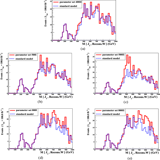
Figure 12: Invariant mass $M(J_{1},recons.W)$ distributions (red-solid) for the five examples [(a) 400II, (b) 500I, (c) 500II, (d) 800I, (e) 800II] together with that of the SM (blue-dotted) for comparison, with ${\sf L}_{int}=$100 fb^-1.

VII Probing Heavy Neutral Higgs Bosons via $\bm{pp\to VH^{\ast}\to VVV}$ associated production

Now we study the process $pp\to VH^{\ast}\to VVV\to\ell^{+}\nu_{\ell}j_{1}j_{2}j_{3}j_{4}$, $V=W,Z$. Here the $W$ boson decaying to $\ell^{+}\nu_{\ell}$ can be either the weak boson associated with $H$ or a weak boson in $H$ decay. The other two weak bosons decay to $j_{1}j_{2}j_{3}j_{4}\sim J_{1}J_{2}$, where $J_{1}$ and $J_{2}$ are two fat jets. From now on, we take a convention regarding $J_{1}$ as the fat jet with largest transverse momentum, and $J_{2}$ as the one with second largest transverse momentum.

The Feynman diagrams for the signal and example of the IB are shown in FIG. 13

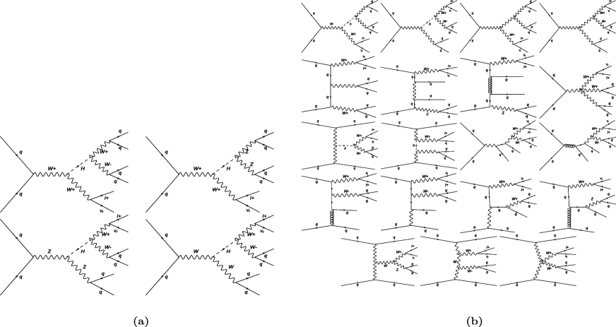
Figure 13: Feynman diagrams in $VH$ associated production. (a) The signal, (b) examples of the IB.

Again, these two amplitudes have interference, so that they should be calculated together.

Next we consider the RBs. Now the largest QCD background is the inclusive $W+2j$ when $W\to\ell^{+}\nu_{\ell}$ and the two jets mimic the two fat jets in the signal. For safety, we take into account all the $W+$ jets and the $W+V+$ jets processes to do the simulation, and pick up the parts that can mimic the signal as the QCD backgrounds. For the top-quark background, we make the same treatment (cf. FIG. 9).

We then make the following kinematic cuts for suppressing the backgrounds.

cut1: Leptonic cuts

Similar to what we did in Sec. II, we require an isolated $\ell^{+}$ ($\mu^{+},e^{+}$) in the detectable rapidity region (cf. TABLE 2), i.e.,

$$N(\ell^{+})=1,~{}~{}~{}~{}N(\ell^{-})=0$$

$${\rm with}~{}~{}~{}~{}~{}~{}~{}~{}~{}~{}~{}~{} \eta_{\ell^{+}}<2.4.$$ (49)

Figure 14: $p_{T}(leptons)$ distributions of signal+IB (red-solid), IB (pink-dotted) and total RBs (blue-small-dotted) in $pp\to VH^{\ast}\to VVV$ process for example 500II with ${\sf L}_{int}=$100 fb^-1.

Next we make the cut on $p_{T}(leptons)$. The inclusive $p_{T}(leptons)$ distributions of the signal plus IB, the RB and the total background are shown in FIG. 14. Here, we do not have to take care of the transverse momentum balance with the forward jets as in Sec. II, so we can take a stronger cut

$$\left|p_{T}(leptons)\right|>400\,{\rm GeV}$$ (50)

to suppress more backgrounds. This cut can also strongly suppress the fake leptons.

cut2: fat jet cuts

As mentioned in Sec. II, we require the first two large transverse momenta to satisfy

$$70\,{\rm GeV}<M(J_{1})<100\,{\rm GeV}$$

$$70\,{\rm GeV}<M(J_{2})<100\,{\rm GeV}.$$ (51)

This can suppress the backgrounds with ordinary jets.

cut3: Top-quark veto

As in Sec. II, for suppressing the top-quark background, we construct two invariant masses $M(J,j_{1})$ and $M(J,j_{2})$, where $J=J_{1}~{}{\rm or}~{}J_{2}$, and $j_{1}$, $j_{2}$ are the two observed jets from the partons $b$ or $\bar{b}$ in FIG. 9. In FIG. 15 we plot the $M(J,j_{1})$ [or $M(J,j_{2})$] distribution from our simulation including the signal plus IB (red-solid) and the top-quark background (blue-dotted) distributions for the example 500II with ${\sf L}_{int}=$100 fb^-1. We can see clearly the top-quark peak (in the blue-dotted curve) in the region $130\,{\rm GeV}<M(J,j)<240\,{\rm GeV}$ for $j$=$j_{1}$ or $j_{2}$.

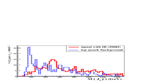
Figure 15: $M(J,j)$ distributions of signal+IB (red-solid) and the top-quark background (blue-dotted) in $pp\to VH^{\ast}\to VVV$ process for the example 500II with ${\sf L}_{int}=$100 fb^-1.

As in Sec. II, we set the cut

$${\rm 130\,GeV}<M(J,j)<{\rm 240\,GeV},$$ (52)

to suppress the top-quark background. We should veto the event if one of $M(J,j_{1})$ and $M(J,j_{2})$ satisfies (52). Equivalently, we only take the events in which both $M(J,j_{1})$ and $M(J,j_{2})$ are outside the region (52). In this way, we can effectively veto the top-quark background events.

cut4: The $\Delta R(\ell^{+},J_{1},)$ cut

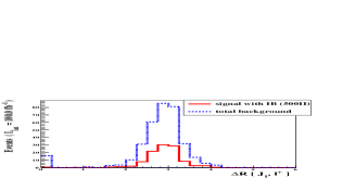
Figure 16: $\Delta R(\ell^{+},J_{1})$ distributions of signal+IB (red-solid) and the total background (blue-dotted) in the $pp\to VH^{\ast}\to VVV$ process for example 500II with ${\sf L}_{int}=$100 fb^-1.

In $VH$ associated production, because $H$ is heavy and has a quite large momentum, the recoil transverse momentum of the associated $V$ boson is generally large. Furthermore, due to the large momentum of the heavy Higgs boson $H$, the angular distance between two weak bosons from $H$ decay is small, while that between the weak boson associated with $H$ and any of the weak boson in $H$ decay is large. If $\ell^{+}$ comes from the $W$ boson associated with $H$, the angular distance between $\ell^{+}$ and any of the fat jets is large. If $\ell^{+}$ comes from the decay of $H$, there must be a fat jet $J_{1}$ (actually from the $V$ boson associated with $H$) with large $\Delta R(\ell^{+},J_{1})$. The background does not have this situation. We plot, in FIG. 16, the $\Delta R(\ell^{+},J_{1})$ distributions of the signal plus IB (red-solid) and the total background (blue-dotted) in the $VH$ associated production for the example 500II with ${\sf L}_{int}=$100 fb^-1. We see that the main distribution of the red-solid curve is indeed located further right to that of the blue-dotted curve. So that a cut

$$\Delta R(\ell^{+},J_{1})>2.5$$ (53)

can suppress the total background.

We know that cut1 on the leptons can effectively avoid the fake leptons from ordinary jets to mimic the signal lepton. However, since the fat jets $J_{1}$ and $J_{2}$ have quite large transverse momenta, cut1 may not be sufficient to suppress the fake leptons from the fat jets. Therefore, we should require the lepton not to overlap with any of the fat jets. Since we have taken $R=0.7$ in jet formations, this means both $\Delta R(\ell^{+},J_{1})$ and $\Delta R(\ell^{+},J_{2})$ should be larger than 0.7. cut4 already guarantees $\Delta R(\ell^{+},J_{1})$ to satisfy this requirement. So that we add the requirement

$$\Delta R(\ell^{+},J_{2})>0.7$$ (54)

here.

Table 5: Cut efficiencies expressed in terms of the tree-level cross sections $\sigma_{S+IB}$ and $\sigma_{B}$ (in units of fb) in the $pp\to VH^{\ast}\to VVV$ process. The first five columns are values of $\sigma_{S+IB}$ for the five examples, and The last four columns are values $\sigma_{B}$ for four kinds of backgrounds.

			$\sigma_{S+IB}$						$\sigma_{B}$
	400II	500I	500II	800I	800II		IB	W+jets	$t\bar{t}$	WV+jets
without cuts	2085	2037	2009	1917	1996		1925	31500000	92000	7600
Cut 1	46.9	54.4	25.7	18.6	25.3		13.1	1422	65.9	47.9
Cut 2	2.78	4.36	1.21	0.629	1.41		0.211	2.91	0.716	0.336
Cut 3	2.32	3.79	1.08	0.526	1.24		0.13	2.15	0.149	0.25
Cut 4	2.04	3.21	0.921	0.426	1.11		0.061	1.39	0.060	0.179

Table 6: Required integrated luminosity ${\sf L}_{int}$ (in units of fb^-1) for the statistical significance of $1\sigma,\,3\sigma$ and $5\sigma$ for the five examples in $pp\to VH^{\ast}\to VVV$ process.

			${\sf L}_{int}$ [fb${}^{-1}]$
	400II	500I	500II	800I	800II
$1\sigma$	0.43	0.18	2.3	13	1.6
$3\sigma$	3.9	1.6	21	115	14
$5\sigma$	10.8	4.5	57	319	39

To see the efficiency of each cut, we list the values of the cross sections (in fb) for signal plus IB (for the five examples mentioned in Sec. I) and various backgrounds after each cut in TABLE 5. We see that, with all these cuts, the backgrounds can be effectively suppressed. Compared with the numbers in TABLE 3, we see that all the backgrounds in TABLE 5 are more suppressed. Again the signal plus IB cross section is of the order of 0.4–3 fb, so that for an integrated luminosity of around 100 fb^-1, we can have a few tens to a few hundreds of events.

From Eqs. (40)–(42), we obtain the required integrated luminosity for the statistical significance of $1\sigma$, $3\sigma$ and $5\sigma$ for the five examples mentioned in Sec. I (cf. TABLE 6).

We see that, except for 800I, all the other four examples are hopeful to be discovered ($5\sigma$) in the first few years run of the 14 TeV LHC; while 800I can have evidence (3$\sigma$) for ${\sf L}_{int}=115$ fb^-1, and can be discovered ($5\sigma$) for ${\sf L}_{int}=319$ fb^-1 at the 14 TeV LHC. These are conclusions considering only the statistical errors.

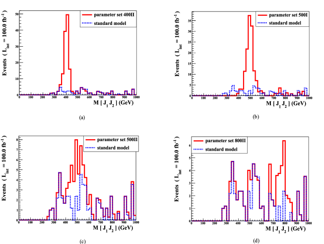
Figure 17: Invariant masses $M(J_{1},J_{2})$ in the $pp\to VH^{\ast}\to VVV$ process after all cuts and $\Delta R(\ell^{+},J_{2})>2.5$ for the examples: (a) 400II, (b) 500I, (c) 500II, and (d) 800II.

Finally, we deal with the issue of experimentally discovering $H$ and measuring $M_{H}$. In addition to cut4, we add a cut

$$\Delta R(\ell^{+},J_{2})>2.5,$$ (55)

where $J_{2}$ is the other fat jet. Then both $J_{1}$ and $J_{2}$ will mainly come from the decay of $H$, and thus the invariant mass $M(J_{1},J_{2})$ will show the $H$ peak at $M(J_{1},J_{2})=M_{H}$. Since the uncertainties in identifying the fat jet from a boosted W boson decay are small CMS_JME_13_006 , measuring the $M(J_{1},J_{2})$ distribution is quite feasible experimentally.

FIG. 17 shows the $M(J_{1},J_{2})$ distributions for examples 400II, 500I, 500II and 800II. We see that sharp peaks can be seen clearly, and thus the heavy Higgs boson and its mass can be detected experimentally. This is the advantage of the $pp\to VH^{\ast}\to VVV$ process.

The example 800I is special. It has a very large decay width due to the largeness of $\Gamma(H\to t{\bar{t}})$, so that there cannot be a sharp peak showing up. However, due to the fact that $M_{H}\gg M_{h}$ in this example, the heavy Higgs boson $H$ moves much more slowly than the light Higgs boson $h$ does. Therefore, $\Delta R(\ell^{+},J_{2})$ for $H$ is larger than that for $h$ in the SM background. In FIG. 18 we plot the $\Delta R(\ell^{+},J_{2})$ distributions of the signal plus IB (red-dotted) and the SM background (dark-solid) in the range $\Delta R(\ell^{+},J_{2})>0.7$ due to (54).

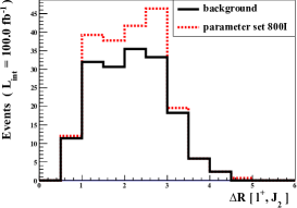
Figure 18: $\Delta R(\ell^{+},J_{2})$ distributions of signal+IB (red-dotted) and the total background (dark-solid) in the $pp\to VH^{\ast}\to VVV$ process for the example 800I with ${\sf L}_{int}=$100 fb^-1.

We see that the main distribution of the signal plus IB is located around $\Delta R(\ell^{+},J_{2})=2.7$ which is right to that of the SM background at around $\Delta R(\ell^{+},J_{2})=2.3$, and the height of signal plus IB is higher. This can be seen as a characteristic feature of the heavy Higgs boson contribution in example 800I.

In principle, we can replace the cut (55) by $\Delta R(J_{1},J_{2})>2.5$ to extract the contribution of the Feynman diagram in which the leptons are from $H$ decay, and use the reconstruction method suggested in Ref. Butterworth to calculate the invariant mass $M(J_{1},recons.W)$ distribution as what we did in FIG. 12. However, our result shows that the obtained resonance peaks are less clear than those in FIG. 17. So we only suggest the method presented above.

From FIG. 17 we see that the excess of events over the SM result is more significant for lighter Higgs boson than for heavier Higgs boson. This is just the opposite to that in the $VV$ scattering process (cf. the last paragraph in Sec. II). This means that the $VV$ scattering process and the $pp\to VH^{\ast}\to VVV$ process are complementary to each other in this respect.

Having found the resonance, the next task is to determine whether its spin is really zero. This can be done by studying the decay mode $H\to ZZ\to 4\ell$ Miller which needs much larger integrated luminosity. Another possible way is to measure the azimuthal angle dependence as suggested by ref. Murayama .

VIII Measuring the Anomalous Coupling Constants $\bm{f_{W}}$ and $\bm{f_{WW}}$

If we can measure the values of the anomalous coupling constants $f_{W}$ and $f_{WW}$ which characterize the heavy neutral Higgs boson $H$, it will be a new high energy measurement of the property of the nature, and will serve as a new high energy criterion for the correct new physics model. All new physics models predicting $f_{W}$ and $f_{WW}$ not consistent with the measured values should be ruled out. The necessary condition for surviving new physics models is that their predicted $f_{W}$ and $f_{WW}$ should be consistent with the measured values. We shall see that this measurement is really possible.

It has been pointed out in Ref. QKLZ09 that, for a single-Higgs system, measuring both the cross section and the leptonic transverse momentum distribution in weak-boson scattering processes may determine the values of $f_{W}$ and $f_{WW}$ to a certain precision. However, in our present case with both $h$ and $H$ contributions, the weak-boson scattering process is not so optimistic for this purpose. So we concentrate on studying the measurement of $f_{W}$ and $f_{WW}$ in the $pp\to VH^{\ast}\to VVV$ process.

VIII.1 The Case of $\bm{M_{H}=500}$ GeV as an Example

Let us take the case of $M_{H}=500$ GeV as an example. After measuring the resonance peak experimentally, we can impose an additional cut

$$400\,{\rm GeV}<M(J_{1},J_{2})<600\,{\rm GeV}$$ (56)

to take the events in the vicinity of the resonance peak to further improve the signal to background ratio. Now we take four sets of the anomalous coupling constants $f_{W}$ and $f_{WW}$, and see if there can be certain new observables to distinguish them. We take

set I: $C_{t}=1,\,\rho_{h}=0.8$, $\rho_{H}=0$, and $f_{W}=f_{WW}=0$
     (background).
set II: $C_{t}=0.6,\,\rho_{h}=0.8$, $\rho_{H}=0.6$ and
     $f_{W}=-f_{WW}=6$ TeV^-2.
set III: $C_{t}=0.6,\,\rho_{h}=0.8$, $\rho_{H}=0.6$, and $f_{W}=12$
     TeV^-2$\gg f_{WW}=0$.
set IV: $C_{t}=0.6,\,\rho_{h}=0.8$, $\rho_{H}=0.6$, and
     $f_{W}=0\ll f_{WW}=12$ TeV^-2.

We can now construct several observables which may be able to distinguish the four sets of $f_{W}$ and $f_{WW}$ listed above, namely (a) the $p_{T}(leptons)$ distribution, (b) the $p_{T}(J_{1})$ distribution, (c) the $\Delta R(\ell^{+},J_{2})$ distribution, and (d) the $\Delta R(J_{1},J_{2})$ distribution. In the two transverse momentum distributions, the additional cuts (56) and $\Delta R(\ell^{+},J_{2})>2.5$ are taken, while in the two angular distance distributions none of these additional cuts is taken.

In FIG. 19 we plot these four distributions for the four sets of $f_{W}$ and $f_{WW}$ with ${\sf L}_{int}=100$ fb^-1, where the dark-solid, red-dotted, pink-dashed, and blue-dashed-dotted curves stand for set I, set II, set III and set IV, respectively.

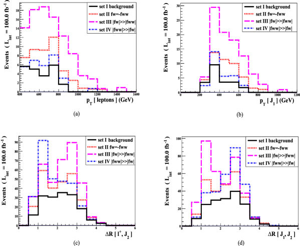
Figure 19: (a) The $p_{T}(leptons)$ distribution [with (56) and $\Delta R(\ell^{+},J_{2})>2.5$] , (b) the $p_{T}(J_{1})$ distribution [with (56) and $\Delta R(\ell^{+},J_{2})>2.5$], (c) the $\Delta R(\ell^{+},J_{2})$ distribution [without (56) and $\Delta R(\ell^{+},J_{2})>2.5$], and (d) the $\Delta R(J_{1},J_{2})$ distribution [without (56) and $\Delta R(\ell^{+},J_{2})>2.5$], with ${\sf L}_{int}=100$ fb^-1. The dark-solid, red-dotted, pink-dashed, and blue-dashed-dotted curves stand for set I, set II, set III and set IV, respectively.

We see that, in all the four distributions, the curves of the four sets can be clearly distinguished. The differences between different sets in FIG. 19(c) and FIG. 19(d) are more significant. Therefore, measuring the four distributions experimentally, and checking with each other, the relative size of $f_{W}$ and $f_{WW}$ existing in the nature can be obtained, and together with the measurement of the cross section, the values of $f_{W}$ and $f_{WW}$ can be separately determined, which gives the new criterion for discriminating new physics models. This is an important advantage of the $pp\to VH^{\ast}\to VVV$ process.

VIII.2 The Case of $\bm{M_{H}=800}$ GeV as an Example

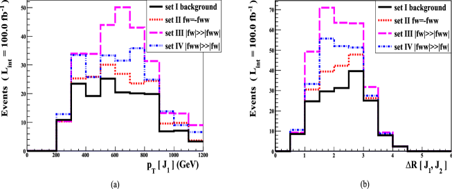
Figure 20: (a) the $p_{T}(J_{1})$ distribution and (b) the $\Delta R(J_{1},J_{2})$ distribution for $M_{H}=800$ GeV with ${\sf L}_{int}=100$ fb^-1. The meaning of the curves is the same as in FIG. 19 but with $C_{t}=1$.

Since in the case of 800I no clear peak can be seen and it can only be realized by the distribution in FIG. 18, we now examine whether it is possible to measure the values of $f_{W}$ and $f_{WW}$ in this case. In FIG. 20 we plot the $p_{T}(J_{1})$ and $\Delta R(J_{1},J_{2})$ distributions for the $M_{H}=800$ GeV case with four sets of parameters as those in the case of $M_{H}=500$ GeV but with $C_{t}=1$. We see that the four sets of $f_{W}$ and $f_{WW}$ can all be clearly distinguished.

IX Summary and Discussion

To search for new physics beyond the SM, we suggest searching for heavy neutral Higgs bosons which are generally contained in new physics models.

We summarize our results as follows.

i     In this paper, we have considered an arbitrary new physics theory containing more than one Higgs bosons $\Phi_{1},\,\Phi_{2},\cdots$ taking account of their mixing effect. For generality, we do not specify the EW gauge group except requiring that it contains an $SU(2)_{L}\times U(1)$ subgroup with the gauge bosons $W,\,Z$ and $\gamma$. We also neither specify the number of $\Phi_{1},\,\Phi_{2},\cdots$, nor specify how they mix to form mass eigenstates except to identify the lightest Higgs boson $h$ to the recently discovered $M_{h}=$125–126 GeV Higgs boson. Then we study the general properties of the couplings of both the lightest Higgs boson $h$ and a heavier neutral Higgs boson $H$ (lighter than other heavy Higgs bosons). The probe of gauge-phobic heavy neutral Higgs bosons are not considered in this study, and will be studied elsewhere.
     We first gave a general model-independent formulation of the couplings of $h$ and $H$ to fermions and gauge bosons based on the idea of the effective Lagrangian up to dim-6 operators in Sec. II. The obtained effective couplings for the Higgs-gauge interaction are different from the traditional ones constructed for a single-Higgs system by containing new parameters $\rho_{h}$ and $\rho_{H}$ reflecting the Higgs mixing effect. After taking account of the constraints from the known low energy experiments, there are seven unknown coupling constants left, namely the gauge coupling constant $\rho_{h}$ in the dim-4 gauge interaction of $h$ [cf. Eq.(II.2)], the gauge coupling constant $\rho_{H}$ in the dim-4 gauge interaction of $H$ [cf. Eq. (II.2)], the anomalous coupling constants $f_{W},\,f_{WW},\,f_{B},\,f_{BB}$ in the dim-6 gauge interactions of $H$ [cf. (10), and (11)], and the anomalous Yukawa coupling constant $C_{t}$ of $H$ [cf. Eq.(̇2)], and the corresponding momentum representations are given in Eqs. (13), (14), (15), (16), (17), and (18).

ii     To estimate the possible range of the anomalous coupling constants $f_{W},\,f_{WW},\,f_{B},\,f_{BB}$, we first studied the theoretical constrains from the requirement of the unitarity of the $S$-matrix of weak-boson scattering in Sec. III. We took the effective $W$ approximation to calculate the scattering amplitudes, and calculate the constraints on $f_{W}$ and $f_{WW}$ by a two-parameter numerical analysis. The obtained constraints are shown in FIG. 2.

iii     We further studied the experimental constraints from the ATLAS and CMS experiments in Sec. IV to obtain further constraints. Anomalous coupling constants consistent with both the unitarity constraints and the experimental constraints are the available anomalous couplings that an existing heavy neutral Higgs boson can have.
  We first make an approximation of neglecting the anomalous coupling constants in the $H\gamma\gamma$ and $HZ\gamma$ couplings inspired by the trend of the ATLAS and CMS measurements of $\mu=\sigma/\sigma_{SM}|_{95\%~{}CL}$ in the decay channels $H\to\gamma\gamma$ and $H\to Z\gamma$. This approximation leads to the constraints (32) and (33) which simplifies our analysis.
  Then we consider the CMS exclusion bounds on the SM Higgs boson for the Higgs mass up to 1 TeV, to obtain the experimental bounds on $f_{W}$ and $f_{WW}$. The calculation is to full leading order in perturbation. We took the cases of 400II, 500I, and 500II as examples. In our calculation of the total decay width of $H$, we have made a conservative approximation. The obtained conservative experimental constraints and the available regions of $f_{W}$ and $f_{WW}$ are shown as the blue shaded regions in FIGs. 3, 4, and 5. This guarantees that a heavy Higgs boson $H$, with its $f_{W}$ and $f_{WW}$ in the blue shaded regions, is definitely not excluded by the CMS exclusion bound CMS_HIG_13_002 . In the cases of 800I and 800II, there is almost no experimental constraint on $f_{W}$ and $f_{WW}$ because the CMS exclusion bound is very loose at $M_{H}=800$ GeV.

iv     In this paper, for studying the LHC signatures of $H$, we suggest taking $VV$ scattering and $pp\to VH^{\ast}\to VVV$ as sensitive processes for probing the anomalous heavy Higgs boson model-independently at the 14 TeV LHC. We take the general model-independent formulation of the heavy Higgs couplings in Sec. II. and take five sets of anomalous coupling constants allowed by the unitarity constraint and the present CMS experimental exclusion bound as examples to do numerical simulation, namely 400II, 500I, 500II, 800I, 800II with the heavy Higgs mass $M_{H}=$ 400 GeV, 500 GeV, and 800 GeV (cf. Sec. IV). The calculations are to the hadron level. We take the CTEQ6.1 parton distribution functions CTEQ6.1 , and use MADGRAPH5 MADGRAPH5 to do the full tree-level simulation. The parton shower and hadronization are calculated with PYTHIA6.4 PYTHIA6.4 , and the anti-$k_{T}$ algorithm with $R=0.7$ antik_T in DELPHES 3 DELPHES3 is used for the formation of jets. We also use DELPHES 3 to simulate the detecting efficiency of the detector.

v     We first study the the semileptonic decay mode of weak-boson scattering, i.e., $pp\to VVj^{f}_{1}j^{f}_{2}\to\ell^{+}\nu_{\ell}j_{1}j_{2}j^{f}_{1}j^{f}_{2}$. The Feynman diagrams of the signal and backgrounds are shown in FIGs. 6–9. The largest background is the QCD background, the inclusive $pp\to W+3j$ which is larger than the signal plus irreducible background (IB) by four orders of magnitude. To suppress the backgrounds, we imposed five kinematic cuts given in Eqs. (43)–(48) which can effectively suppress the backgrounds. The cut efficiencies of each cut are listed in TABLE 3, and the required integrated luminosities for $1\sigma$ deviation, $3\sigma$ evidence, and $5\sigma$ discovery are shown in TABLE 4. It shows that examples 500II and 800II are hopeful to be discovered (at the $5\sigma$ level) in the first few years run of the 14 TeV LHC. while 800I can be discovered (at the $5\sigma$ level), and 400I and 500I can have evidence (at the $3\sigma$ level) for an integrated luminosity of 300 fb ^-1 at the 14 TeV LHC. We then took the method of determining the longitudinal momentum of the neutrino by requiring to reconstruct the $W$ boson mass correctly Butterworth , and with which we calculated the invariant mass $M(J_{1},recons.W)$ distributions as shown in FIG. 12. We see that there are evident excesses of events over the SM result around $M(J_{1},recons.W)=M_{H}$. This can be the signal of the contribution of the intermediate state heavy Higgs boson. We also see that the excess of events are more significant for heavier Higgs boson than for lighter Higgs boson.

vi     We then study the semileptonic mode of the $pp\to VH^{\ast}\to VVV$ process, $pp\to VH^{\ast}\to VVV\to\ell^{+}\nu_{\ell}j_{1}j_{2}j_{3}j_{4}\to\ell^{+}\nu_{\ell}J_{1}J_{2}$ ($J_{1}$ and $J_{2}$ stand for the fat jets with largest and second largest transverse momenta, respectively). The Feynman diagrams for the signal and IB are shown in FIG. 13. Reducible backgrounds include $W+2$-$jet$, and the top-quark background similar to those in the weak-boson scattering process. We also imposed five kinematic cuts in Eqs. (49)–(54). The cut efficiencies after each cut are listed in TABLE 5 which shows that all backgrounds are more effectively suppressed. The required integrated luminosities for $1\sigma$ deviation, $3\sigma$ evidence, and $5\sigma$ discovery are shown in TABLE 6. Except for the example 800I, all the other four examples are hopeful to be discovered ($5\sigma$ level) in the first few years run of the 14 TeV LHC; while 800I can have an evidence (3$\sigma$) for ${\sf L}_{int}=115$ fb^-1, and can be discovered ($5\sigma$) for ${\sf L}_{int}=319$ fb^-1 at the 14 TeV LHC. In FIG. 17, we plot the invariant mass distributions $M(J_{1},J_{2})$ for examples 400II, 500I, 500I, and 800II, which shows that the resonance peaks for all these four examples are clearly seen. This makes it possible for the experimental search for the heavy Higgs boson $H$ and the measurement of its mass $M_{H}$. For the example 800I, due to the large decay rate of $\Gamma(H\to t{\bar{t}})$, the total decay width of $H$ is very large such that there is no clear peak showing up. However, FIG. 18 shows a characteristic feature of the $M_{H}=800$ GeV Higgs boson in the $\Delta R(\ell^{+},J_{2})$ distribution, which can help the experiment to find out the contribution of the heavy Higgs boson $H$. We see that the excess of events are more significant for lighter Higgs boson than for heavier Higgs boson. This is just the opposite to the case of the $VV$ scattering. So, in this sense, the $VV$ scattering process and the $pp\to VH^{\ast}\to VVV$ process are complementary to each other.
  After determining the spin of the resonance, one can confirm the discovery of a heavy Higgs boson.

vii     We also show the possibility of measuring the values of anomalous coupling constants $f_{W}$ and $f_{WW}$ experimentally by measuring both the cross section and the $p_{T}(leptons)$ distribution, the $p_{T}(J_{1})$ distribution, the $\Delta R(\ell^{+},J_{2})$ distribution, and the $\Delta R(J_{1},J_{2})$ distribution (cf. FIGs. 19 and 20). This will be a new measurement of the property of the nature at high energies, and will serve as a new high energy criterion for the correct new physics model. All new physics models predicting $f_{W}$ and $f_{WW}$ not consistent with the measured values should be ruled out. The necessary condition for surviving new physics models is that their predicted $f_{W}$ and $f_{WW}$ should be consistent with the measured values.

In weak-boson scattering, we imposed the forward-jet cut $p_{T}(j^{f})>35$ GeV to avoid the pile-up events, while we did not impose that in $VH$ associated production. This is because the transverse momenta of all the final state particles are large, e.g., our simulation shows that $p_{T}(J_{2})>100$ GeV, $p_{T}(J_{1})>200$ GeV [cf. FIG. 19(b)], and $p_{T}(leptons)>400$ GeV [cf. Eq. (50)].

In all our predictions, only the statistical error is considered. We leave the study of the systematic error related to the details of the detectors to the experimentalists. Moreover, with the study of the jet shape, it may further suppress the backgrounds BDRS Han09 .

In Ref. Englert the 1-loop level contribution $gg\to VH$ in the SM was studied, and they showed that, although it is smaller than the tree-level quark initiated contribution, this contribution can help to enhance the signal in $VH$ associated production. This may also enhance the signal in our $pp\to VH^{\ast}\to VVV$ process. However, in our Type-II examples, $C_{t}<1$, so that the gluon initiated contribution is less important.

Finally we make a check of the unitarity of our calculation. We know that the values of the anomalous couplings $f_{W}$ and $f_{WW}$ which we take in this paper are consistent with the unitarity constraints (FIG. 2). However, the unitarity constraints are obtained in the effective $W$ approximation. Here we make a more realistic check based on our full simulation. In FIG. 21, we plot three invariant mass distributions up to a few TeV at the LHC in the $VV$ scattering and the $pp\to VH^{\ast}\to VVV$ processes. We see that, in the high energy region, all distributions are monotonically decreasing to zero. This shows that there is no unitarity violation, so that our calculation is consistent with the unitarity requirement.

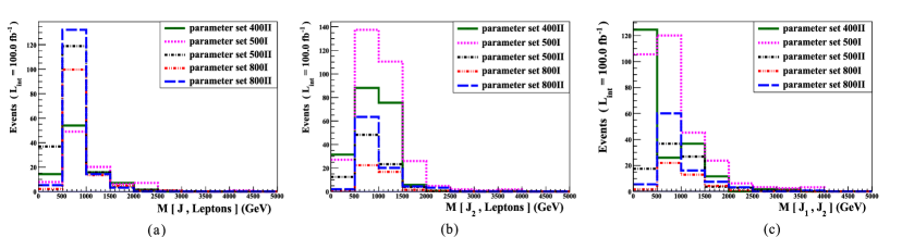
Figure 21: Check of unitarity: (a) $M(J,leptons)$ distribution in weak-boson scattering, (b) $M(J_{2},leptons)$ distribution and (c) $M(J_{1},J_{2})$ distribution in the $pp\to VH^{\ast}\to VVV$ process.

Acknowledgement We are grateful to Xin Chen for valuable discussions. We would also like to thank Tsinghua National Laboratory for Information Science and Technology for providing their computing facility. This work is supported by the National Natural Science Foundation of China under the grant numbers 11135003 and 11275102.

References

- (1) G. Aad et al. (ATLAS Collaboration), Phys. Lett. B 716, 1 (2012); S. Chatrchyan et al. (CMS Collaboration), Phys. Lett. B 716, 30 (2012).
- (2) S. Chatrchyan et al. (CMS Collaboration), JHEP 06, 81 (2013); S.M. Consonni et al. (ATLAS Collaboration), arXiv: 1305.3315.
- (3) For instance, the International Linear Collider (ILC), the Future Circular Collider (FCC) proprosed at CERN, and the Circular Electron-Positron Collider CEPC proposed in China.
- (4) R. Dashen and H. Neuberger, Phys. Rev. Lett. 50, 1897 (1983).
- (5) L. Susskind, Phys. Rev. D 20, 2619 (1979).
- (6) A.A. Savin (CMS Collaboration), Recent results on beyond the standard model Higgs bosons searches from CMS, arXiv: 1201.4983.
- (7) S.M. Consonni (ATLAS Collaboration), Higgs Searches at ATLAS, arXiv: 1305.3315.
- (8) G. Aad et al. (ATLAS Collaboration), Phys. Rev. D 89, 032002 (2014).
- (9) There have been papers studying the constraints on the anomalous couplings of the discovered Higgs boson from the existing LHC data leading to the conclusions that the anomalous couplings of this Higgs boson are consistent with zero at the CL, and more data are needed. For example, Tyler Corbett, O.J.P Eboli, J. Gonzalez-Fraile, and M.C Gonzalez-Garcia, Phys. Rev. D 87, 015022 (2013); ibid 86, 075013 (2012); C. Englert, et al., arXiv: 1403.7191.
- (10) CMS Collaboration, Report No. CMS-PAS-HIG-13-002 (unpublished).
- (11) CMS Collaboration, Report No. CMS-PAS-HIG-12-024 (unpublished).
- (12) CMS Collaboration, Report No. CMS-PAS-HIG-13-014 (unpublished).
- (13) S. Chatrchyan et al. (CMS Collaboration), JHEP 01, 096 (2014).
- (14) CMS Collaboration, Report No. CMS-PAS-HIG-13-008 (unpublished).
- (15) K. Hagiwara, S. Ishihara, R. Szalapski, and D. Zeppenfeld, Phys. Rev. D 48, 2182 (1993).
- (16) Let us consider if higher dimension operators can be introduced. We first look at the dim-5 operator . We can write it as . The first term (total derivative) contributes only on the surface at infinity so that can be dropped. For the second and third terms, the Dirac equation reduces them to which is just the Yukawa form. So the dim-5 operator is actually equivalent to the dim-4 operator for on-shell fermions. It has been argued that the dim-6 operators also do not lead to new forms A_S , as we are not interested in the multi-Hggs-fermion couplings which is irrelevant to our study. This is why we only take the Yukawa form here.
- (17) J.A. Aguilar-Saavedra, Nucl. Phys. B821, 215 (2009).
- (18) W. Buchmüller and D. Wyler, Nucl. Phys. B268, 621 (1986); C.J.C. Burges and H.J. Schnitzer, Nucl. Phys. B228,464 (1983); C.N. Leung, S.T. Love, and S. Rao, Z. Phys. C 31, 433 (1986).
- (19) For a review, see M.C. Gonzalez-Garcia, Int. J. Mod. Phys. A 14, 3121 (1999).
- (20) Bin Zhang, Yu-Ping Kuang, Hong-Jian He, and C.P. Yuan, Phys. Rev. D 67, 114024 (2003).
- (21) V. Barger, T. Han, P. Langacker, B. McElrath, and P.M. Zerwas, Phys. Rev. D 67, 115001 (2003).
- (22) For example, G. Aad et al. (ATLAS Collaboration), Eur. Phys. J. C 72, 2173 (2012); S. Chatrchyan et al. (CMS Collaboration), Eur. Phys. J. C 73, 2610 (2013).
- (23) G.J. Gounaris, J. Layssac, and F.M. Renard, Phys. Lett. B 332,146 (1994); G.J. Gounaris, J. Layssac, J.E. Paschalis, and F.M. Renard, Z. Phys. C 66, 619 (1995).
- (24) M. Jacob and G.C. Wick, Ann. Phys. 7, 404 (1959).
- (25) See, e.g., Refs. CMS_HIG_13_002 and CMS12024 . The CMS exclusion bounds in other Higgs decay channels are all weaker. See, e.g., Ref. CMS13014 , Ref. CMS2013_221 and Ref. CMS13008 .
- (26) N.D. Christensen and C. Duhr, Comput. Phys. Commun. 180, 1614 (2009).
- (27) J. Alwall, M. Herquet, F. Maltoni, O. Mattelaer and T. Stelzer, JHEP 06, 128 (2011).
- (28) G. Aad et al. (ATLAS Collaboration), Phys. Rev. Lett. 108, 111803 (2012).
- (29) CMS Collaboration, Report No. CMS-PAS-HIG-13-001 (unpublished).
- (30) ATLAS Collaboration, Report No. CERN-PH-EP-2014-006 arXiv: 1402.3051.
- (31) S. Chatrchyan et al. (CMS Collaboration), Phys. Lett. B 726, 587 (2013).
- (32) Y.-H. Qi, Y.-P. Kuang, B.-J. Liu, and B. Zhang, Phys. Rev. D 79, 055010 (2009).
- (33) J. de Favereau et al., JHEP 02, 057 (2014), arXiv: 1307.6346.
- (34) D. Stump et al., JHEP 10, 046 (2003).
- (35) T. Sjöstrand, S. Mrenna, and P. Skands, JHEP 05, 026 (2006).
- (36) M. Cacciari, G.P. Salam, and G. Soyez, JHEP 04, 063 (2008).
- (37) S. Chatrchyan al., (CMS Collaboration), J. Instr. 6, 11002 (2011).
- (38) J. Beringer et al., (Partical Data group), Phys. Rev. D 86, 010001 (2012).
- (39) J. Bagger, V. Barger, K. Cheung, J. Gunion, T. Han, G.A. Ladinsky, R. Rosenfeld and C.P. Yuan, Phys. Rev. D 49, 1246 (1994). Phys. Rev. D 52, 3878 (1995).
- (40) J.M. Butterworth, B.E. Cox, and J.R. Forshaw, Phys. Rev. D 65, 096014 (2002).
- (41) Recently the CMS Collaboration made an analysis of identifying the fat jet from boosted W boson decay at the 8 TeV LHC (cf. The CMS Collaboration, Identification techniques for highly boosted W bosons that decay into hadrons, CMS-JME-13-006, arXiv: 1410.4227v1.) showing that the uncertainty is less than . The situation may be further improved in the 14 TeV run.
- (42) M.L. Mangano, M. Moretti, and R. Pittau, Nucl. Phys. B 632, 343 (2002).
- (43) J. Alwall et al., Eur. Phys. J. C 53, 473 (2008).
- (44) CMS collaboration. Search for a Standard Model-like Higgs boson decaying into WW lqq in pp collisions at = 8 TeV. CMS-PAS-HIG-13-008 (2013).
- (45) The CMS Collaboration, Search for Resonances in Semileptonic Top Pair Production at TeV, CMS PAS TOP-11-009.
- (46) D.J. Miller e͡t al., Phys. Lett. B 505, 149 (2001).
- (47) M.R. Buckley, H. Murayama, W. Klemm, and V. Rentala, Phys. Rev. D 78, 014028 (2008).
- (48) J.M. Butterworth, A.R. Davison, M. Rubin, and G.P. Salam, Phys. Rev. Lett. 100, 242001 (2008).
- (49) T. Han, D. Krohm. L.T. Wang. and W. Zhu, arXiv: 0911.3656.
- (50) C. Englert, M. MaCullough, and M. Spannowsky, Phys. Rev. D 89, 013013 (2014).