Sigma-terms and axial charges for hyperons and charmed baryons

Abstract:

We present results for the $\sigma$-terms and axial charges for various hyperons and charmed baryons using $N_{f}=2+1+1$ twisted mass fermions. For the computation of the three-point function we use the fixed current method. For one of the $N_{f}=2+1+1$ ensembles with pion mass of 373 MeV we compare the results of the fixed current method with those obtained with a stochastic method for computing the all-to-all propagator involved in the evaluation of the three point functions.

1 Introduction

The nucleon axial charge $g_{A}$ is a well-measured quantity extracted from neutron $\beta$- decay experiments. The nucleon light $\sigma_{\pi N}$ term is extracted from $\pi N$ scattering phase shifts combining experimental measurements and phenomenology. The nucleon strange content $\sigma^{s}$ is extracted in a similar manner using the kaon $N$ scattering phase shifts, which however are difficult to measure and, furthermore, chiral perturbation theory may not be applicable. For other particles, these quantities are either poorly known or their values are not known experimentally. Assuming SU(3) flavor symmetry one can obtain useful relations among the axial charges of hyperons. Such relations are used as input in low-energy effective theories [1, 2] and it is therefore important to test the degree of their validity. Lattice QCD provides the appropriate framework to calculate these quantities for all baryons. In this work, we thus focus on computing the $\sigma$ -terms and axial charges for hyperons and charmed baryons.

While the evaluation of the nucleon axial charge $g_{A}$ has been carried out by a number of lattice QCD collaborations [3] the axial charges of other baryons are not so well studied. The focus of this work is to evaluate the axial charges and $\sigma$-terms, which are extracted from matrix elements at zero momentum transfer. Since we are interested in evaluating matrix elements for any baryon, the fixed current method is the appropriate approach yielding with one sequential inversion per quark flavor the axial charges of all baryons. An additional sequential inversion per quark flavor is carried out to extract the $\sigma$-terms. In order to avoid additional sequential inversions are for every operator we study a new method for computing hadron matrix elements using a stochastic method to calculate the all-to-all propagator entering the three-point function. We will refer to this alternative method as the stochastic method, which is extremely versatile as compared to either the fixed sink or fixed current approaches conventionally employed in three-point function computations. The advantage of the stochastic method is that once the all-to-all propagator is computed one can obtain the matrix elements of any hadron and for any operator.

2 Tuning the strange and charm quark mass

We use $N_{f}=2+1+1$ twisted mass fermions (TMF) configurations simulated at $\beta=1.95$. The action we employ introduces a twisted heavy mass-split doublet for the strange and the charm quark

$$S_{F}^{(h)}[\chi^{(h)},\bar{\chi}^{(h)},U]=a^{4}\sum_{x}\bar{\chi}^{(h)}(x)\left(D_{W}[U]+m_{0}+i\mu_{\sigma}\gamma_{5}\tau^{1}+\tau^{3}\mu_{\delta}\right)\chi^{(h)}(x)\>,$$ (1)

where $m_{0}$ is the bare untwisted quark mass, $\mu_{\sigma}$ is the bare twisted mass along the $\tau^{1}$ direction and $\mu_{\delta}$ is the mass splitting in the $\tau^{3}$ direction [4]. For the valance sector we use Osterwalder-Seiler fermions and, therefore, we need to tune the strange and charm mass. The tuning is performed by matching the mass of the kaon and D-meson in the tuunitary and mixed action setups. To perform the matching we vary the mass of the strange and charm quarks and fit the resulting masses using the following polynomial form [5]

$$a^{2}M_{PS}^{2}(a\mu_{l},a\mu_{h})=a_{1}(\mu_{l}+\mu_{h})+a_{2}(\mu_{l}+\mu_{h})^{2}+a_{3}(\mu_{l}+\mu_{h})^{3}+a_{4}(\mu_{l}+\mu_{h})(\mu_{l}-\mu_{h})^{2}\,,$$ (2)

where $\mu_{l}$ is the mass of the u- and d- quarks as used in the simulation and $\mu_{h}$ is varied in a range that includes the kaon and D-meson mass. The resulting fit can be seen in Fig. 1 covering the whole range of masses from the kaon to the D-meson mass. As a consistency check we also perform a fit to a smaller range in $a\mu_{h}$ close to the kaon mass using $a^{2}M_{PS}^{2}(a\mu_{s})=c_{1}+c_{2}a\mu_{s}$ and independently around the D-meson mass using $aM_{PS}(a\mu_{c})=d_{1}+d_{2}a\mu_{c}$ as shown in the right panel of Fig. 1. We find $a\mu_{s}=0.01671(18)(28)$ and $a\mu_{c}=0.2195(15)(10)$, where the first error is statistical and the second systematic determined as the difference between the value extracted from the polynomial fit over the whole range of heavy masses and the one extracted from the linear fit over the range shown in the right panel in Fig. 1.

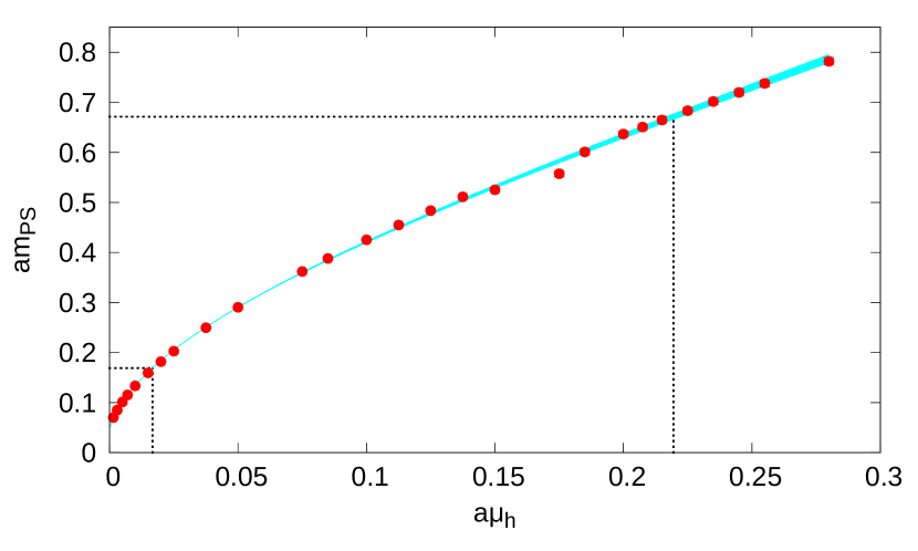
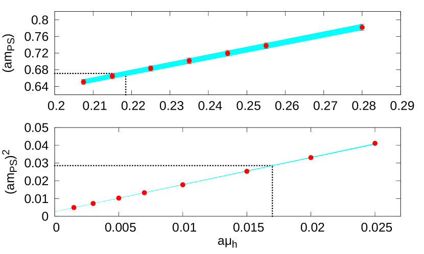
Figure 1: Pseudoscalar mass as a function of $a\mu_{h}$. Left: Fit to the polynomial given in Eq.(2.2). Right: Linear fit around the range of the kaon mass (upper) and around the D-meson mass (lower).

3 Axial charges

The axial charge $g_{A}$ is a fundamental quantity of the structure of a hadron. Within lattice QCD the calculate the axial charge for any hadron, is extracted from the matrix element of the axial-vector current, $A^{3}_{\mu}\equiv\bar{\psi}(x)\gamma_{\mu}\gamma_{5}\psi(x)$ at zero momentum transfer: $\langle h(\vec{p}^{\prime})|A_{\mu}|h(\vec{p})\rangle$. $SU(4)$ flavor symmetry leads to two 20-plets of spin-1/2 and spin-3/2 baryons, for which we calculate the axial charges using the interpolating field given in Ref. [2] including a spin-3/2 projection, which is found to be important in the case of the $\Xi^{*}$s. Assuming SU(3) flavor symmetry the axial charges of the low-lying octet baryons obey the following relations [1]

$$g_{A}^{N}=F+D,\,\,g_{A}^{\Sigma}=2F,\,\,g_{A}^{\Xi}=-D+F\,\,\Longrightarrow\,\,\delta_{\rm SU(3)}\equiv g_{A}^{N}-g_{A}^{\Sigma}+g_{A}^{\Xi}=0.$$ (3)

We examine how well SU(3) flavor symmetry is satisfied for unequal quark masses by computing the SU(3) symmetry breaking parameter $\delta_{\rm SU(3)}$. In Fig. 2 we plot $\delta_{\rm SU(3)}$ as a function of the dimensionless parameter $x=(m_{K}^{2}-m_{\pi}^{2})/(4\pi^{2}f_{\pi}^{2})$. In the plot we include results obtained using a hybrid action of staggered fermions and domain wall valence quark that includes a calculation at the SU(3) flavor symmetric limit [6]. Performing a chiral extrapolation using $\delta_{\rm SU(3)}=ax^{2}$ we find that the deviation from SU(3) flavor symmetry at the physical value of the strange quark mass is around $10\%$.

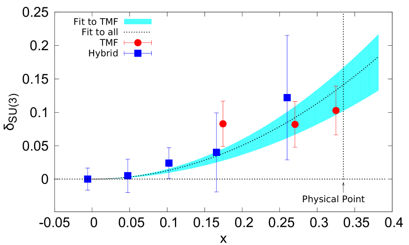
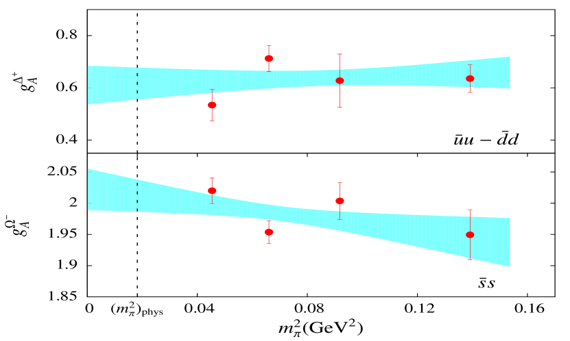
Figure 2: Left: $\delta_{\rm SU(3)}$ versus $x=(m_{K}^{2}-m_{\pi}^{2})/(4\pi^{2}f_{\pi}^{2})$. Filled red circle are TMF results and filled blue squares are results using a hybrid action [6]. Right: Isovector axial charge of the $\Delta^{+}$ and the connected contribution to the strange axial charge of the $\Omega^{-}$ versus $m_{\pi}^{2}$.

One can also compute the axial charges of baryons belonging to the decuplet. We show in Fig. 2 two representative examples of the light and strange quark contribution to the axial charge of the $\Omega^{-}$ and the $\Delta^{+}$ computing only the connected contributions. For $\Omega^{-}$ the value increases as we approach the physical pion mass. A linear fit to $m_{\pi}^{2}$ yields a good fit to the data and provides a prediction of the strange axial charge of these baryons.

Using the same techniques we compute the axial charges of charmed baryons whose values are not known. The interpolating fields are given in Ref. [7].

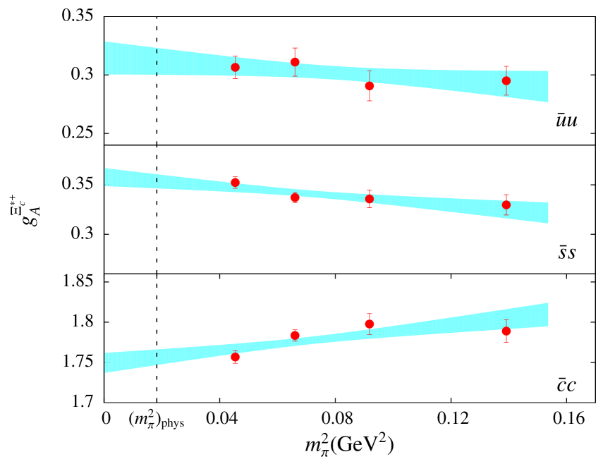
Figure 3: The axial charge as a function of $m_{\pi}^{2}$ for $\Xi^{*+}_{c}$ (left) and $\Omega^{*+}_{cc}$ (right).

We show in Fig. 3 two representative examples of the strange and charm quark contribution to the axial charge of the $\Xi^{*+}_{c}$ and the $\Omega^{*+}_{cc}$ as a function of $m_{\pi}^{2}$. An interesting feature is that the light and strange quark contributions to th e axial charge of charmed baryons increase as the pion mass approaches the physical value while for the charm content decreases.

4 $\sigma$-terms

Experimental searches for cold dark matter need as input the strength of the interaction between a WIMP and a nucleon mediated by a Higgs exchange. Thus a reliable calculation of the nucleon $\sigma$-terms provides an important input for these experiments. There are phenomenological determinations of the value of $\sigma_{\pi N}$, as well as, lattice QCD calculations mainly using the Feynman-Hellman theorem [8], but also by directly calculating the nucleon matrix element $\sigma_{\pi N}=m_{l}\langle N|\bar{u}u+\bar{d}d|N\rangle$ [9, 10]. In this work, we compute the matrix element $\sigma_{q}=m_{q}\langle h|\bar{\psi}\psi|h\rangle$ for all low-lying baryons belonging to the two 20-plets of SU(4).

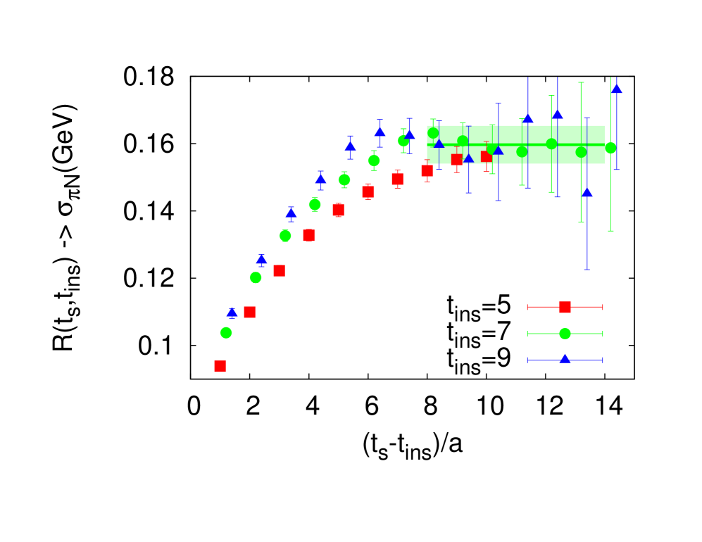
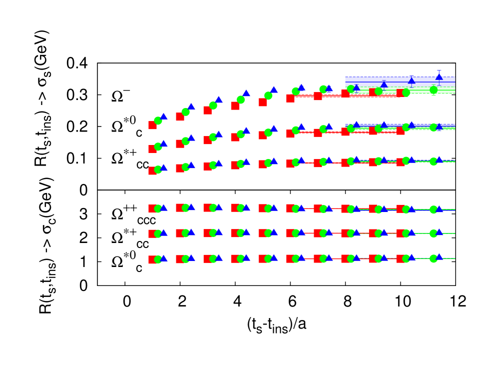
Figure 4: The ratio $R(t_{ins},t_{s})$ which yields the $\sigma$-term as a function of $(t_{s}-t_{ins})/a$ for the nucleon (left) and for the strange (upper) and charm (lower) content of the $\Omega$s (right).

In Fig. 4 we show the ratio of the three-point function to the two point function $R(t_{ins},t_{s})=\frac{G^{3pt}(\Gamma,t_{ins},t_{s})}{G^{2pt}(t_{s})}$ for representative cases for the light, strange and charm quark content, considering only connected contributions. In the fixed current approach one needs to fix the time separation between current insertion and source, taken at zero, $t_{ins}$. Since this observable, unlike the axial charge, receives large excited state contributions we need to ensure that $t_{ins}$ is sufficiently large so that the excited states are damped out before we extract the value of $\sigma$ by fitting to a constant. We show the ratio as a function of $t_{s}-t_{ins}$ in Fig. 4 for three values of $t_{ins}$. As can be seen $t_{ins}=7a$ yields consistent results with those for $t_{ins}=9a$. This is true for $\sigma_{\pi n}$, as well as, for the strange and charm content of the $\Omega$s. Thus, we fix $t_{ins}=7a$. In Fig. 4 we show the strange quark contribution to the $\Omega^{-}$ which has three strange quarks, $\Omega^{*0}_{c}$ with two strange quarks and $\Omega^{*+}_{cc}$ with one strange quark. As can be seen the strange quark contribution triples for $\Omega^{-}$ as compared to $\Omega^{*+}_{cc}$ as expected. The same is true also for the case of the charm contribution to the $\sigma$-term.

5 Stochastic Method for connected diagrams

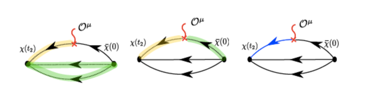
Figure 5: Fixed sink (left), fixed insertion (center) and stochastic method (right). With green lines we depicted the part of the diagram which is used as a source for the sequential inversion and with yellow the sequential propagator.

In Fig. 5 we show diagrammatically the fixed sink and current methods that are used in the calculation of three-point functions. The former requires us to fix the sink i.e. the hadron state and the latter the operator insertion. In order to be able to compute the three-point function for every hadron state and current insertion we examine a third approach that computes the all-to-all stochastically [11]. Within this approach the all-to-all propagator is written in terms of a solution vector $\phi(x)$ and a noise vector $\xi(y)$ with the consequence that the double sum involved in the calculation of three point functions becomes two single sums:

$$\sum_{\vec{y}}\sum_{\vec{x}}e^{-i\vec{p}^{\prime}\cdot\vec{x}}e^{-i\vec{p}\cdot\vec{y}}G(x;y)\Gamma G(y;0)\longrightarrow\\ \frac{1}{N_{r}}\sum_{r=1}^{N_{r}}\left(\sum_{\vec{x}}e^{-i\vec{p}^{\prime}\cdot\vec{x}}\phi_{r}(x)\right)\left(\sum_{\vec{y}}e^{-i\vec{p}\cdot\vec{y}}\xi^{*}_{r}(y)\Gamma G(y;0)\right).$$ (4)

This makes the calculation via the stochastic method feasible, provided the number of noise vectors $N_{r}$ needed is small enough. In Fig. 6 we compare results using the stochastic method to those obtained using the fixed sink method. The comparison is done using 500 gauge configurations of $N_{f}=2+1+1$ TMF at pion mass $373$ MeV. We invert at every $t_{s}$ (time dilution) and consider spin and color dilution. Thus for a given $t_{s}$ we need 12 inversions per noise vector which is the same as the number of inversions need to obtain the sequential propagator.

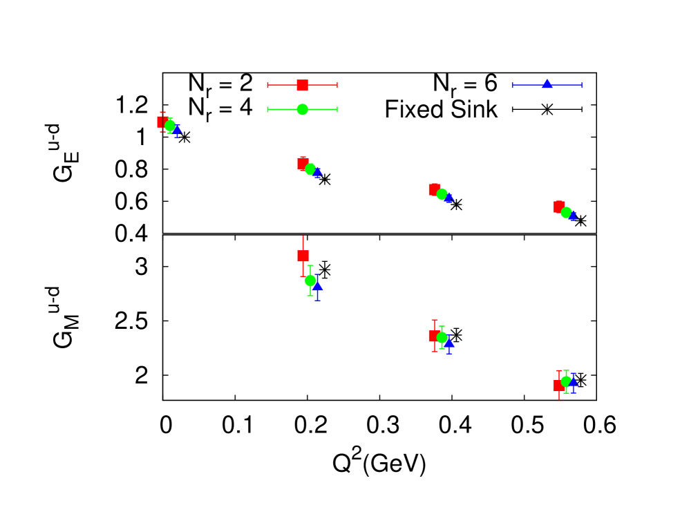
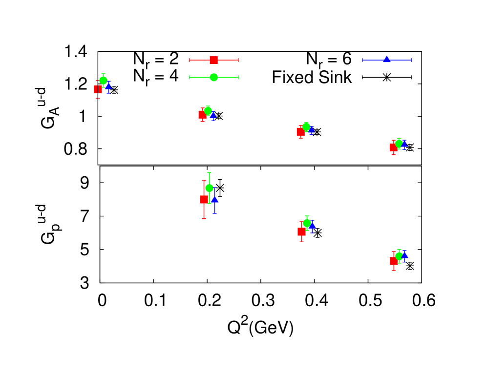
Figure 6: Electromagnetic (left) and axial (right) form factors versus $Q^{2}$.

In Fig. 6 we show results on the nucleon electromagnetic and axial-vector form factors using $N_{r}=2,4$ and 6. The results obtained using the stochastic method show good convergence obtaining when using $N_{r}=4$ and $N_{r}=6$ values that are consistent with those obtained with the fixed sink method for all cases except the electric form factor, which requires $N_{r}=6$. Taking $N_{r}=6$, means that the stochastic method needs six times more inversions to achieve the accuracy of the fixed sink method. However, the stochastic method is more versatile and we can extract more measurements without additional inversions that over-compensate for this factor of six. To understand the gain we consider the cost needed to evaluate the axial form factors.

	Projectors	States	# $N_{r}$	# Inversions	Err(Stoch)/Err(Fixed Sink)
Fixed Sink	$\sum_{k=1}^{3}\Gamma_{k}$	$p$	-	$24$	-
Stochastic	$\sum_{k=1}^{3}\Gamma_{k}$	$p$	$2$	$2\times 24$	$\thicksim 3$
Stochastic	$\Gamma_{1},\Gamma_{2},\Gamma_{3}$	$p,n$	$2$	$2\times 24$	$\thicksim 1$

Table 1: The number of inversions and the resulting ratio of the error of the stochastic method to that of the fixed sink method for the summed and unsummed spin projectors $\Gamma_{k}$.

In the case of the stochastic method to use three different projector $\Gamma_{k}$, $k=1,\cdots,3$ needs no extra inversions unlike the fixed-sink method. In Table 1 we compare the results obtained using the summed projector $\sum_{k=1}^{3}\Gamma_{k}$ with the fixed sink method, which requires one inversion per quark flavor, with those obtained using the stochastic method. We find about 3 times the error when using the stochastic method with $N_{r}=2$, which is twice as expensive as the fixed sink method. However, in the stochastic method we can use the unsummed projector, which carries less noise than the summed one, and average over proton and neutron without extra cost reducing the error by a factor of about 3. Thus, in the case the nucleon the cost is twice that of the fixed sink technique for a fixed error. Thus, considering even only two hadron states we break even. Given that we can compute all form factors for the 40 SU(4) particles with no additional inversions shows the superiority of the stochastic method.

6 Conclusions

In this work we present results on the $\sigma$-terms and axial charges for the two SU(4) 20-plet baryons. We study the SU(3) flavor breaking and the behavior of the $\sigma$-terms as we vary the number of quarks. For the extraction of the axial charges and $\sigma$-terms we use the fixed current method. To avoid the limitations of the fixed current or sink methods which additional inversions for each operator or hadron state (spin projection) respectively we tested a stochastic method to calculate the all-to-all propagator involved in the computation of connected three-point function. This method shows a very fast convergence to the results of the fixed sink method, and for the case of the nucleon axial charge, it is only twice as expensive. Therefore, it can be considered as an alternative approach for the calculation of three-point functions, in particular when we are interested in matrix elements of more than one hadron.

References

- [1] B. C. Tiburzi and A. Walker-Loud, Phys. Lett. B 669, 246 (2008) [arXiv:0808.0482 [nucl-th]].
- [2] C. Alexandrou et al. [ETM Collaboration], Phys. Rev. D 80, 114503 (2009) [arXiv:0910.2419].
- [3] C. Alexandrou, PoS LATTICE 2010, 001 (2010) [arXiv:1011.3660 [hep-lat]].
- [4] R. Baron et al., JHEP 1006, 111 (2010) [arXiv:1004.5284 [hep-lat]].
- [5] B. Blossier et al. [ETM Collaboration], JHEP 0804, 020 (2008) [arXiv:0709.4574].
- [6] H. -W. Lin and K. Orginos, Phys. Rev. D 79, 034507 (2009) [arXiv:0712.1214 [hep-lat]].
- [7] C. Alexandrou et al., Phys. Rev. D 86, 114501 (2012) [arXiv:1205.6856 [hep-lat]].
- [8] R. D. Young, PoS LATTICE 2012, 014 (2012) [arXiv:1301.1765 [hep-lat]].
- [9] C. Alexandrou et al., PoS LATTICE 2012, 163 (2012) [arXiv:1211.4447 [hep-lat]].
- [10] C. Alexandrou et al., arXiv:1309.7768 [hep-lat].
- [11] C. Alexandrou et al. [ETM Collaboration], arXiv:1302.2608 [hep-lat].