Accelerated post-AGB evolution, initial-final mass relations, and the star-formation history of the Galactic bulge

Abstract

Aims. We study the star-formation history of the Galactic bulge, as derived from the age distribution of the central stars of planetary nebulae that belong to this stellar population.

Methods. The high resolution imaging and spectroscopic observations of 31 compact planetary nebulae are used to derive their central star masses. We use the Blöcker post asymptotic giant branch (post-AGB) evolutionary models, which are accelerated by a factor of three in this case to better fit the white dwarf mass distribution and asteroseismological masses. Initial-final mass relations (IFMR) are derived using white dwarfs in clusters. These are applied to determine original stellar masses and ages. The age distribution is corrected for observational bias as a function of stellar mass. We predict that there are about 2000 planetary nebulae in the bulge.

Results. The planetary nebula population points at a young bulge population with an extended star-formation history. The Blöcker tracks with the cluster IFMR result in ages, which are unexpectedly young. We find that the Blöcker post-AGB tracks need to be accelerated by a factor of three to fit the local white dwarf masses. This acceleration extends the age distribution. We adjust the IFMR as a free parameter to map the central star ages on the full age range of bulge stellar populations. This fit requires a steeper IFMR than the cluster relation. We find a star-formation rate in the Galactic bulge, which is approximately constant between 3 and 10 Gyr ago. The result indicates that planetary nebulae are mainly associated with the younger and more metal-rich bulge populations.

Conclusions. The constant rate of star-formation between 3 and 10 Gyr agrees with suggestions that the metal-rich component of the bulge is formed during an extended process, such as a bar interaction.

1 Introduction

The origin and evolution of the Galactic bulge (GB) of the Milky Way is an area of active research. Bulges were believed to be similar to elliptical galaxies with a proposed origin in minor mergers. This was supported by the relation between bulge/spheroid luminosities and central black-hole masses (Graham, 2007). However, some bulges are more disk-like in their properties and these have been termed ’pseudo-bulges’: their origin is likely unrelated to those of the spheroidal bulges (Kormendy & Kennicutt, 2004). Pseudo-bulges can form by secular evolution over a longer period, while classical bulges are predominantly an early product of galaxy formation.

Whether the Milky Way bulge is a classical or pseudo-bulge is disputed. There is evidence for old stellar populations. Vanhollebeke et al., (2009) compared OGLE and 2MASS data to the galactic model TRILEGAL to find good fits for models with a starburst from 8 to 10 Gyr ago with the best fit for the younger age. The metallicity is close to solar with a distribution extending not very far towards lower values. In recent years, however, the evidence for a younger stellar component has been growing. In a recent review, Babusiaux, (2012) concluded that the other characteristics point toward a mix of stellar populations although the main shape of the GB seems to be driven by secular evolution. This multi-component structure is also seen in the shape of the GB (Robin et al., 2012), which may be a combination of a classical and a pseudo (box-shape) bar.

Regarding the age and duration of star-formation in GB, Tsujimoto & Bekki, (2012) concluded that the metal-poor and metal-rich populations are formed at different times with the former extending over 2 Gyr and the latter over 4 Gyr. This separation was also found by Bensby et al., (2010, 2011, 2013). They carried out spectroscopy of GB dwarf stars during gravitational lensing amplification events. Stellar parameters were derived based on LTE model atmospheres, and stellar ages were interpolated from a grid of isochrones. Bensby et al. found that stars with sub-solar metallicities are predominantly old (around 10 Gyr) as expected in the GB. At super-solar metallicities, however, they find a wide range of ages with a peak around 5 Gyr and a tail towards higher ages. They conclude that the origin of the GB is still poorly constrained and speculate that the young stars might be the manifestation of the inner thin disk. Gonzalez et al., (2011) also found evidence for a separate, high metallicity component of the bulge, which they attribute to stars originating from the thin disk.

Planetary nebulae (PN), which are bright and easy to identify, can help us to address the question of the age of the Galactic bulge. The PNe trace populations which have ages ranging from $<1$ to 10 Gyr. In contrast, red clump data analysis, as used by Robin et al., (2012), cannot discriminate any ages over 5 Gyr. However, deriving ages for the central stars of individual PNe has been a challenge.

In this paper, we investigate the relation between the stellar populations and the planetary nebula population of the Galactic bulge by deriving the initial masses and, therefore, the ages of the PN central stars. This makes use of new Hubble Space telescope (HST) images and complementary Very Large Telescope (VLT) high-resolution spectra to find the mass distribution of the central stars of bulge planetary nebulae. These are converted to initial masses using initial-final mass relations (IFMR); the stellar ages are found using the stellar mass-age relations. The central star mass distribution can be compared with a well-known distribution of white dwarf masses and the age distribution can be compared with ages of bulge stars.

The steps are critically dependent on post asymptotic giant branch (post-AGB) stellar evolution models and the IFMR. We show that a recalibration of the speed in the post-AGB evolution is required to reproduce the well-known distribution of white dwarf masses. The IFMR is used as a free parameter to fit known bulge ages. The final conversion to a star-formation history also requires corrections for observational bias. After these corrections, we find that the results are consistent with an extended epoch of bulge formation.

The paper is organized as follows. Section 2 presents the collected observational material and its analysis with photoionization models. In Sect. 3, masses of central stars of PNe are derived and compared to the known white dwarf masses. The discrepancies can be resolved with a proposed acceleration of post-AGB evolution. In Sect. 4, the stellar initial masses and ages from the zero-age main sequence (ZAMS) are derived using a newly-derived IFMR and some evolutionary model tracks. Section 5 considers the effect of selection and PN visibility bias. Finally, the adjusted age distribution of the GB PNe is derived in Sect. 6, where we use the IFMR as a free parameter. When compared to other published bulge age determinations, it points towards a rather steep IFMR.

2 Observations and analysis

2.1 The HST images

We obtained SNAPshot HST/WFPC2 images of compact bulge PNe (program 9356). The data were obtained in 2002 and 2003 and comprised of images in three different filters: F656N, F547M, and F502N for a total of one HST orbit (96 min including overheads) per object. The pixel scale of the camera is 0.0455 arcsec.

To get as close as possible to a randomly selected sample for this SNAPshot survey, we first identified all compact bulge PNe in the ESO/Strasbourg catalogue (Acker et al., 1992) with a reported diameter of less than 5 arcsec or of unknown diameter. Sixty objects were randomly selected from this list, which is about half the total number. These were entered in the SNAPshot survey without further prioritization. Based only on schedulability, 37 of these were actually observed. One target turned out to be too faint for further analysis. This leaves a sample of 36 compact objects, representing the GB PNe population. It forms an unbiased selection from the compact PNe in the Acker catalogue and is not based on any brightness or morphological information. Inevitably, it is still affected by discovery biases inherent in the original catalogue.

2.2 VLT/UVES long-slit spectra

A series of 600-second VLT/UVES (Dekker et al., 2000) echelle spectra were obtained in 2005 with a slit 0.5 arcsec wide and 11 arcsec long. The slit was put through the centres of the nebulae, which are aligned with the brightest structures. In most cases, the slit was aligned with the minor axis, and the spectra therefore represent the densest part of the nebula. The observations cover a spectral region approximately from 3300 to 6600 Å. The spectral resolution of 60 000 resolves the line profiles, allowing us to determine the velocity structure of the expanding nebula.

The ESO Common Library (CPL) pipeline was applied (version 4.1.0), which included correction for bias, flat field, wavelength calibration, and order merging. Special attention was required for the order merging process, as there is usually no continuum in PN spectra. The long-slit spectra are spatially resolved in most cases, however, only the central arcsecond was extracted for further analysis as the most representative for the whole PN.

2.3 Photoionization modelling of the nebulae

To model the spectra and line profiles, we applied the Torun photo-ionization codes (Gesicki & Zijlstra, 2003; Gesicki et al., 2006). The star is assumed to be a black body with luminosity and an effective temperature. The nebula is approximated as a spherical shell defined by a radial density distribution and a radial velocity field. The chemical composition and the observed line intensities were adopted from the literature. For most of the PNe, the chemical abundances were recently published by Chiappini et al., (2009) and Górny et al., (2009), while some data were used from Stasińska et al., (1998). These abundances were used in the photo-ionization model. The oxygen data are given in Table 1.

The photo-ionization code calculates a 1-dimensional (radial) emissivity profile. Assuming spherical symmetry, this is converted to the observed projected intensity profile and fitted to the HST images. For this purpose, slices through the images were extracted by running across the brightest areas, which usually correspond to the minor axis (Details are presented in the online Appendix.). This gave not only the outer radius but also an approximation to the density profile. Once a good fit is obtained from the images and the line flux ratios, we add a radial velocity profile to the model nebula. The emissivities are integrated along the line of sight to produce a model line profile at each position. Profiles of lines with different ionization states, which trace different radii within the nebula, are fitted to obtain the radial velocity profile of the nebula. Finally, an average expansion velocity $V_{\rm aver}$ is calculated weighted over the ionized mass at each radius.

Four objects indicated turbulent motions within the nebula, which complicates the velocity interpretation. The lines of different species show similar line widths with a more Gaussian line shape than normally seen. The widening can be modelled with a turbulent velocity component, but the physical meaning of this is not clear. The presence of extra velocity components makes the derivation of the mass-averaged expansion velocity more uncertain. The four objects were therefore excluded from the sample. One object, Th4-1, was unresolved in HST, and we were unable to converge on an acceptable fit. This object was also removed.

The remaining sample of 31 PNe is uniform and covered by high quality data, which benefits the modelling. The objects are at nearly the same distance, which allows for robust luminosity and dimensions estimations. All objects have spatially resolved HST images. Because of the very high angular resolution of these images, the radial intensity profiles are well determined, and these, in turn, are used to derive the radial dependency of the density. The high resolution spectra provide a number of emission lines, which cover a reasonably wide range of ionization and excitation.

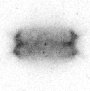
Figure 18: The nebula H 2-37 (PN G 002.3$-$03.4). The data are presented as in Fig. 17.

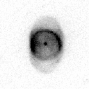
Figure 19: The nebula H 2-20 (PN G 002.8+01.7). The data are presented as in Fig. 17.

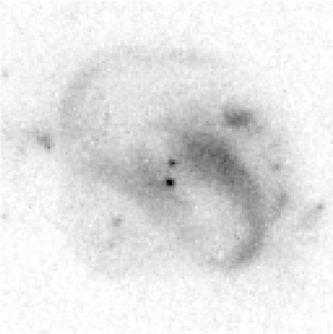
Figure 20: The nebula H 2-39 (PN G 002.9-03.9). The data are presented as in Fig. 17. In spite of the complex structure, the velocity profile is well reproduced by the 1-D model.

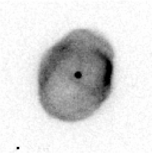
Figure 21: The nebula H 2-17 (PN G 003.1+03.4). The data are presented as in Fig. 17.

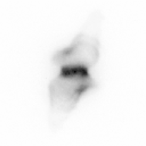
Figure 22: The nebula M 2-14 (PN G 003.6+03.1). The data are presented as in Fig. 17. The slit is along the minor axis. The high velocity wing of the [N ii] line is not in the model (which assumes a linear velocity gradient). It may arise from the base of the polar flow.

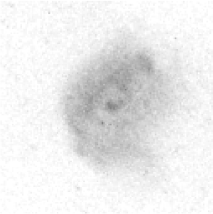
Figure 23: The nebula H 2-15 (PN G 003.8+05.3). The data are presented as in Fig. 17.

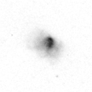
Figure 24: The nebula KFL 11 (PN G 004.1$-$03.8). The data are presented as in Fig. 17. The [N ii] profile is one sided, indicating an asymmetry in the nebula, which is also evident from the image. However, the velocity field is well fitted.

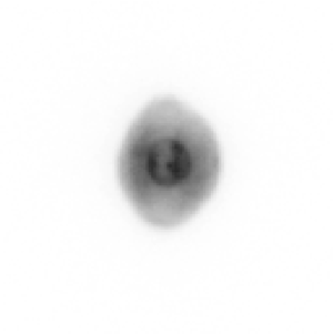
Figure 26: The nebula M 1-20 (PN G 006.1+08.3). The data are presented as in Fig. 17.

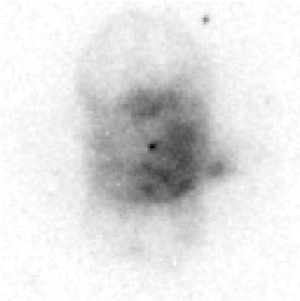
Figure 27: The nebula H 2-18 (PN G 006.3+04.4). The data are presented as in Fig. 17.

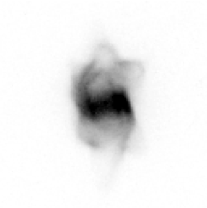
Figure 28: The nebula M 1-31 (PN G 006.4+02.0). The data are presented as in Fig. 17.

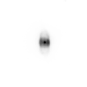
Figure 29: The nebula He 2-260 (PN G 008.2+06.8). The data are presented as in Fig. 17.

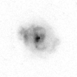
Figure 30: The nebula MaC 1-11 (PN G 008.6$-$02.6). The data are presented as in Fig. 17. The [N ii] line shows a velocity asymmetry, which may also be just visible in [O iii]. The model fits the red-shifted velocities.

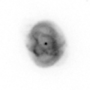
Figure 31: The nebula M 1-19 (PN G 351.1+04.8). The data are presented as in Fig. 17.

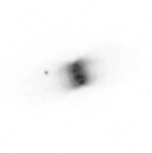
Figure 32: The nebula Wray 16-286 (PN G 351.9-01.9). The data are presented as in Fig. 17. The slit was oriented along the major axis.

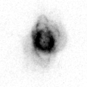
Figure 33: The nebula H 1-8 (PN G 352.6+03.0). The data are presented as in Fig. 17.

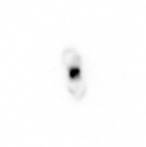
Figure 34: The nebula Th 3-4 (PN G 354.5+03.3). The data are presented as in Fig. 17.

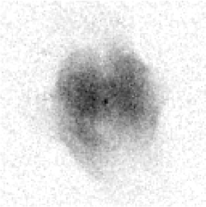
Figure 35: The nebula Th 3-6 (PN G 354.9+03.5). The data are presented as in Fig. 17.

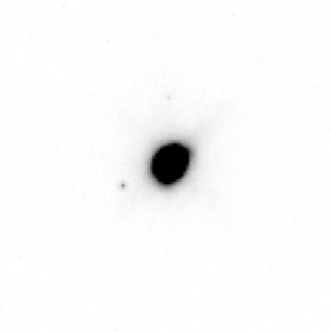
Figure 36: The nebula H 1-9 (PN G 355.9+03.6). The data are presented as in Fig. 17. The radial profile is shown scaled by a factor of 100. The nebula is very compact and the model does not fit the radial distribution well, but the outer radius of the model closely aligns with the edge of the image, as seen in the figure.

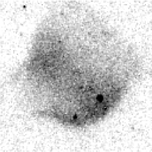
Figure 37: The nebula H 2-26 (PN G 356.1-03.3). The data are presented as in Fig. 17.

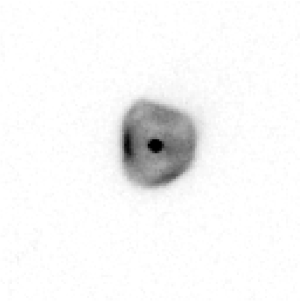
Figure 47: The nebula Th 3-14 (PN G 359.2+04.7). The data are presented as in Fig. 17. There is no [O iii] detected: the spatial profile appears to show stellar continuum only.

For all selected PNe, the most representative observations with the fitted models are presented in the online Appendix. The HST images, VLT/UVES emission lines, and model radial runs are shown in Figs. 17–47. The online Table LABEL:pne_ratios presents more details of the fitted photoionization models.

2.4 Nebular age determination

The kinematical age of the nebula can be obtained from the outer radius divided by its expansion velocity. The outer radius is well determined through the HST images (in the H$\alpha$ line observed with filter F656N, see the Figs. 17–47). However, the velocity at this precise point cannot be measured spectroscopically. Instead, we use the mass-averaged expansion velocity, which is well-determined from the observations and models. It is derived from the hydrogen density distribution and the velocity field of the ionized region.

The expansion rate of the PN outer radius accelerates over time, at least as long as the central star heats up. This has been shown in hydrodynamical modelling by Schönberner et al. (2005) and confirmed observationally for bulge PNe by Richer et al., (2008, 2010). The velocity field inside the nebular shell typically shows increasing velocities with radius with the highest gas velocity found at the outer edge. The outer radius is the location of a shock and expands at the shock propagation speed. The mass-weighted expansion velocity is thus lower than the expansion rate of outer radius. We use the hydrodynamical models of Perinotto et al., (2004) to calibrate the relation between the average expansion velocity, the radius, and the age. These models present self-consistent calculations of the evolution of a PN on a post-AGB track with full coverage of radiation transport, ionization, and hydrodynamics. We calculate the mean propagation speed by dividing the outer radius by the age of the model nebula. The ratio between this and the mass-averaged velocities gives the correction factor, which should be applied.

We applied this procedure to a number of models (kindly provided by the authors) with a nebula evolving around stars of mass $0.565\,M_{\sun}$ and $0.605\,M_{\sun}$ which are the most comparable to our sample. A consistent and well-defined ratio of $1.4\pm 0.1$ is found. This agrees well with the correction factor to the expansion parallaxes of Schönberner et al. (2005), which are derived from the shell where most of the gas resides. The mass-averaged velocity follows the general acceleration trend and is well-approximated by a constant correction factor within this accuracy. Thus,

$$t_{\rm kin}=\frac{R_{\rm out}}{1.4\times V_{\rm aver}}.$$ (1)

The results of the analysis for the 31 objects are listed in Table 1. The temperatures refer to the black-body photo-ionization temperatures for the stars. The nebular radius is measured from the HST images by assuming a distance to the bulge of 8 kpc.

Table 1: Galactic bulge PNe model results and literature data for analysed nebulae. The black-body temperature comes from photoionization modelling. The outer radius corresponds to the equatorial direction seen in the images observed with HST. The kinematical reconstruction provided the mass-averaged velocity and kinematical age. The methods for obtaining cspn masses in standard and accelerated cases are discussed in the text.

PN G	name	$\log T_{\rm bb}$	$R_{\rm out}$	$V_{\rm aver}$	$t_{\rm kin}$	$M_{\rm cspn}$	$M_{\rm cspn}^{\rm accele}$	O/H	ref.
		[K]	[pc]	[km s-1]	[kyr]	[$M_{\sun}$]	[$M_{\sun}$]	12+log$x$
001.7-04.4	H 1-55	4.53	0.07	26	1.88	0.603	0.565	8.45	1
002.3-03.4	H 2-37	5.07	0.12	29	2.89	0.628	0.590	8.06	1
002.8+01.7	H 2-20	4.50	0.065	29	1.57	0.607	0.569	9.26	2
002.9-03.9	H 2-39	5.04	0.11	39	1.97	0.639	0.601	8.41	1
003.1+03.4	H 2-17	4.49	0.08	24	2.33	0.592	0.555	7.44	2
003.6+03.1	M 2-14	4.63	0.045	16	1.96	0.609	0.571	8.56	3
003.8+05.3	H 2-15	4.89	0.12	17	4.93	0.596	0.558	8.66	2
004.1-03.8	KFL 11	4.76	0.08	22	2.54	0.609	0.572	8.39	1
004.8+02.0	H 2-25	4.49	0.10	18	3.88	0.575	0.537	8.33	3
006.1+08.3	M 1-20	4.81	0.044	16	1.92	0.623	0.585	8.53	3
006.3+04.4	H 2-18	4.71	0.11	46	1.67	0.620	0.583	8.56	1
006.4+02.0	M 1-31	4.68	0.04	19	1.47	0.623	0.585	8.91	1
008.2+06.8	He 2-260	4.44	0.02	12	1.16	0.613	0.575	8.00	3
008.6-02.6	MaC 1-11	4.80	0.08	28	2.00	0.621	0.583	-
351.1+04.8	M 1-19	4.71	0.06	23	1.82	0.618	0.580	8.62	3
351.9-01.9	Wray 16-286	4.92	0.06	13	3.22	0.613	0.575	8.74	3
352.6+03.0	H 1-8	4.83	0.07	23	2.13	0.621	0.583	8.76	3
354.5+03.3	Th 3-4	4.68	0.016	19	0.59	0.655	0.617	8.21	3
354.9+03.5	Th 3-6	4.63	0.08	16	3.49	0.589	0.551	-
355.9+03.6	H 1-9	4.55	0.04	21	1.33	0.617	0.579	8.30	1
356.1-03.3	H 2-26	5.18	0.11	20	3.84	0.627	0.588	8.34	2
356.5-03.6	H 2-27	4.81	0.12	25	3.35	0.604	0.566	-
356.8+03.3	Th 3-12	4.51	0.03	9	2.33	0.594	0.556	-
356.9+04.4	M 3-38	5.09	0.02	9	1.55	0.651	0.613	8.39	1
357.1-04.7	H 1-43	4.26	0.04	27	1.03	0.604	0.566	8.12	1
357.2+02.0	H 2-13	4.95	0.09	8	7.86	0.585	0.547	-
358.5-04.2	H 1-46	4.75	0.04	14	2.00	0.618	0.579	8.27	1
358.5+02.9	Al 2-F	4.95	0.08	28	2.00	0.632	0.594	-
358.7+05.2	M 3-40	4.73	0.06	22	1.90	0.618	0.580	-
358.9+03.4	H 1-19	4.67	0.05	17	2.05	0.610	0.572	8.26	3
359.2+04.7	Th 3-14	4.32	0.04	15	1.86	0.588	0.550	-
Abundance references:   (1) Górny et al., (2009); (2) Stasińska et al., (1998); (3) Chiappini et al., (2009).

3 Stellar final masses

In this section, we discuss the method of deriving masses of central stars of PNe (cspn). We pay special attention to the derivation of the lowest masses, where some known cspn masses are lower than predicted by models.

3.1 Post-AGB model tracks

The post-AGB evolution shows rapid heating of the star. The heating rate can be measured from the stellar temperature and the nebula age. The post-AGB models show that this heating rate is a sensitive measure of the stellar mass.

We use the standard set of evolutionary tracks for post-AGB stars obtained by Blöcker, (1995), which are supplemented with lower-mass models from Schönberner, (1983). Alternative post-AGB model tracks are presented by Vassiliadis & Wood, (1994) and Weiss & Ferguson, (2009). We assume that the post-AGB stars evolve as hydrogen burners. Stars in the helium burning phase have lower luminosities and evolve slower. Only a minor fraction of post-AGB stars are expected to be helium burners.

The circumstellar matter is ejected at the tip of the asymptotic giant branch. The cessation of this ejection is defined as the end of the AGB. The time between the end of the AGB and the time when the star reaches $T_{\rm eff}=10^{4}\,$K is commonly called the transition time. Values for the transition times differ enormously between different models. The Blöcker tracks predict transition times that agree with observational constraints (referring mainly to IR observations, see Blöcker, (1995) and the review of Schönberner & Blöcker, (1993)). The models of Weiss & Ferguson, (2009) are particularly fast and the Vassiliadis & Wood, (1994) (VW94) tracks are very slow. The transition time is not always predicted by models: sometimes, it is necessary to remove the envelope ’manually’ and resume the models from $T_{\rm eff}=10^{4}\,$K (Weiss & Ferguson, 2009).

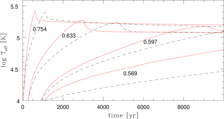
Figure 1: Comparison of four interpolated Blöcker 1995 post-AGB tracks (solid, red lines) with Vassiliadis & Wood, (1994) post-AGB tracks (dashed, in black) of the same mass. Each set of models are labelled with the core mass. The VW94 tracks are shifted to the same age as the corresponding Blöcker track at $T_{\rm eff}=10^{4}$ K to correct for the different transition times.

The heating rate after the transition time depends on the assumed post-AGB mass loss, where the Blöcker tracks and VW94 used a different approach. Figure 1 compares the post-AGB Blöcker tracks with the tracks VW94 for four different stellar masses. The VW94 are shifted in time to start at the same age as the Blöcker track at $T=10^{4}$ K. In all four cases, the VW94 tracks show slower heating rates for the same mass. In other words, the VW94 tracks require higher core masses for the same heating rate (Zijlstra et al., 2008).

3.2 Empirical evolution

3.2.1 Asteroseismological masses

To constrain the models, it is important to directly measure masses of central stars of planetary nebulae to a high accuracy. This has only recently become possible, using asteroseismology on pulsating central stars. Althaus et al., (2010) lists eight such central stars of PNe with measured masses. They are reproduced in Table 2. Five stars have masses around 0.53–0.55 $M_{\sun}$. The remainder are more massive.

Because PNe are seen around these stars the age since the end of the AGB must be $\lesssim 20\,$kyr. For two of the stars in Table 2, we can calculate the kinematical age. For A 43, we find 8.5 kyr and for VV 47 13 kyr, using the data of Friederich et al., (2011) and Weinberger, (1989), respectively. For the last object, we adopt the higher expansion velocity derived from [N ii] rather than lower value from [O iii], as assumed earlier by Schönberner & Napiwotzki, (1990) because [N ii] emission better probes the outer shell regions (e.g., Schönberner et al. 2005). We do not have a mass-averaged velocity for either object, and the kinematical ages are less certain than for the modelled nebulae. However, the numbers confirm that the ages are less than 20 kyr.

Table 2: Asteroseismology masses of PNe central stars of pulsation type PG 1159 from Althaus et al., (2010).

object	name	$T_{\rm eff}$ [K]	$M_{\rm cspn}$ [$M_{\sun}$]
PN G 274.3+09.1	Longmore 4	120	0.63
PN G 036.0+17.6	Abel 43	110	0.53
PN G 066.7$-$28.2	NGC 7094	110	0.53
PN G 118.8$-$74.7	NGC 246	150	0.75
PN G 080.3$-$10.4	RX J2117.1+3412	170	0.72
PN G 094.0+27.4	K 1-16	140	0.54
PN G 104.2$-$29.6	Jn 1	150	0.55
PN G 164.8+31.1	VV 47	130	0.53

The Blöcker models do not predict PNe around such low mass stars. Their post-AGB evolution is extremely slow with the 0.546 $M_{\sun}$ track (Schönberner, 1983) taking $3\times 10^{5}$ yr to reach a peak temperature. The stars of Table 2 are all PG1159 stars, which are hydrogen-poor and believed to have undergone a late thermal pulse during the post-AGB evolution (Miller Bertolami & Althaus, 2006). Their current evolution therefore differs from that of the hydrogen-burning tracks considered here. However, although the late pulse rejuvenates the star, it does not rejuvenate the nebula. The presence of the old PN still sets a minimum speed of evolution during the preceding hydrogen-burning post-AGB phase, and the issue remains that the nebulae are much younger than predicted by the model tracks.

3.2.2 White dwarf masses

A separate constraint on the evolutionary tracks can be obtained by comparing the mass distribution of central stars derived from the Blöcker tracks with the known mass distribution of white dwarfs. White dwarf masses are not known for the Galactic bulge because their low luminosity allows for spectroscopic analysis of objects that are not very distant. The local DA white dwarf mass distribution peaks at $0.576\,M_{\sun}$ (Kepler et al., 2007). Recently, this value has been confirmed by Giammichele et al., (2012): their histogram was plotted with large bins of $0.05\,M_{\sun}$; however, the published catalogue reveals a pronounced maximum at $0.58\,M_{\sun}$. In contrast, PN central star masses, as derived above and in Gesicki & Zijlstra, (2007), peak at values above 0.6 $M_{\sun}$. It has proven difficult to reconcile the distributions. The systematic error in the core masses (discussed in Gesicki & Zijlstra, 2007) is around 0.02 $M_{\sun}$; however the masses in that paper were already shifted down by assuming slow expansion of the nebulae.

To reconcile the models and observations, one can (i) assume a systematic error in the white dwarf and pulsational masses, (ii) limit PN formation to the more massive progenitor stars, or (iii) accelerate the post-AGB tracks to allow lower masses stars to form PNe. Option (i) is less likely, while option (ii) contradicts the presence of PNe around low-mass PG1159 stars, the presence of PNe in the old stellar populations of elliptical galaxies (Arnaboldi, 2011), and the Galactic bulge.

In the next subsections, we therefore investigate a way to (iii) accelerate the post-AGB model tracks.

3.3 Blöcker track interpolation

The Blöcker and Schönberner tracks are calculated for a set of distinct masses. Gesicki & Zijlstra, (2007) interpolated between the individual tracks to derive a denser model grid. In this interpolation, the strongest constraint on the low-mass central stars comes from the Schönberner model of 0.546 $M_{\sun}$. This model evolves so slow that it is off the scale when compared to our kinematical ages, and in the interpolation, this sets a lower limit for the central stars masses at 0.55 $M_{\sun}$. Schönberner, (1983) comments that the 0.546 $M_{\sun}$ model shows evidence for helium burning. The 0.546 $M_{\sun}$ model is an early-AGB model before the onset of thermal pulses, when helium burning contributes significantly to the luminosity (Schönberner, 1983). The very slow evolution is a consequence of this.

We therefore leave out the 0.546 $M_{\sun}$ model from the interpolation. Instead, we use the higher mass tracks to extrapolate towards the low-mass regime. The interpolated formula for cspn masses uses a linear fit in the log(time) – log(temperature) plane:

$$M_{\rm cspn}=0.074\times\log(T_{\rm eff})-0.08\times\log(t_{\rm kin})+0.29.$$ (2)

This is fitted to the horizontal part of four Blöcker tracks (0.565, 0.605, 0.625, and 0.696 $M_{\sun}$). The limited number of data points warrants only a low-order extrapolation. The uniformity of the published tables is very helpful, as each track has the same number of points up to the maximum stellar temperature of each track. The Pikaia genetic algorithm was used to locate the coefficients of the best fit. The maximum difference between the track data points at their horizontal parts and the masses from the simple formula is less than 2%. This formula neglects the cooling part of the evolutionary tracks. However, its advantage is that it allows for easy re-scaling, for example to check how any acceleration of the evolution might affect the derived masses.

3.4 Envelope mass

The second adjustment we can make is to systematically accelerate the evolutionary tracks. This reduces the derived core masses and can thus improve the match to the white dwarf mass distribution.

A physical mechanism for an acceleration of the tracks comes from adjusting the envelope mass at the end of the AGB. This is one of the parameters, which comes from the chosen mass-loss prescription, and is not known a priori. The heating rate is set by the rate at which this envelope mass is removed through hydrogen burning ($\dot{M}_{\rm H}$) and a post-AGB ($\dot{M}_{\rm w}$) wind:

$$\Delta t_{\rm H}\approx\frac{M_{\rm env}^{\rm pAGB}-M_{\rm env}^{T\rm max}}{\dot{M}_{\rm H}+\dot{M}_{\rm w}},$$ (3)

where the envelope mass is measured at the end of the transition time, $M_{\rm env}^{\rm pAGB}$, and the time of maximum temperature (the ’knee’ in the HR diagram), $M_{\rm env}^{T\rm max}$.

The relation of the maximum temperature, $T_{\rm max}$, (in Kelvin) to the envelope mass $M_{\rm env}^{T\rm max}$ (in solar masses) is obtained from a fit to Fig. 4 of Blöcker, (1995):

$$\log{T_{\rm max}}\approx-0.37\times\log{M_{\rm env}^{T\rm max}}+3.83.$$ (4)

The Blöcker tracks also indicate an approximate relation between the core mass and $T_{\rm max}$. We extend the mass range covered by the Blöcker models by using the PN central stars with asteroseismological masses, which reach temperatures of 130 kK for $M_{\rm c}=0.53\,M_{\sun}$ (Althaus et al., 2010). (The lower mass models in Schönberner, (1983) do not reach such high temperatures.) From Fig. 4 in Blöcker, (1995) and the data in Althaus et al., (2010), we find

$$\log T_{\rm max}\approx 1.2\times M_{\rm c}+4.5$$ (5)

for $T$ in Kelvin and $M_{\rm c}$ in solar masses. Combining this with the previous equation give:

$$\log M_{\rm env}^{T\rm max}\approx-3.24\times M_{\rm c}-1.81.$$ (6)

All models in Blöcker, (1995) show a decrease by about $\Delta\log M_{\rm env}=-0.6$ (about a factor of 1/4) from the end of the transition time to the time of maximum temperature:

$$M_{\rm env}^{\rm pAGB}=4\times M_{\rm env}^{\rm Tmax}.$$ (7)

These dependencies of $T_{\rm max}$, $M_{\rm env}^{\rm pAGB}$ and $M_{\rm env}^{T\rm max}$ are illustrated in Fig. 2 (solid lines).

If we assume that post-AGB mass loss rates are much less than the nuclear burning rates, as found for the lower mass models by Blöcker, (1995), then the envelope mass $M_{\rm env}$ decreases with the rate,

$$\dot{M}_{\rm env}\propto L.$$ (8)

The core-mass luminosity relation (in solar units) is given by (Herwig et al., 1998):

$${L}=62200\left({M_{\rm c}}-0.487\right).$$ (9)

Finally, from a fit of Fig. 4 of Blöcker, (1995), we find that the envelope mass at $T=10^{5}$ K is approximately related to the envelope mass at peak temperature:

$$\log\frac{M_{\rm env}^{T5}}{M_{\rm env}^{T\rm max}}=-0.65\times\left(\log T^{\rm max}-5\right),$$ (10)

where $M_{\rm env}^{T5}$ is the envelope mass at $T=10^{5}$ K.

Figure 2: Dependence of the post-AGB maximum temperatures $T_{\rm max}$ and envelope masses on the core mass, based on the relations in Section 3.4. The solid lines show the parametrization, which are fitted to the Blöcker models. The short-dashed lines show the result of reducing the envelope masses at the end of the transition phase by a factor of three. In the bottom panel, we show the envelope mass at the start of the post-AGB evolution and at the time of maximum stellar temperature.

Figure 3: Dependence of the post-AGB time scales on core mass, based on the relations in Section 3.4. The vertical axis shows the time at which maximum temperature is reached. The drawn line (with squares) shows the parametrization, fitted to the 0.605 $M_{\sun}$ Blöcker model. The short-dashed line (with squares) shows the result of reducing the envelope masses at the end of the transition phase by a factor of three. The filled circles show the Blöcker model set, the filled triangles models from Weiss & Ferguson, (2009), and the open octagons show the locations of A 43 and VV 47.

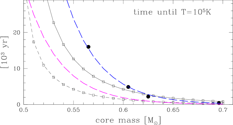
Figure 4: The post-AGB time scale for the star to reach $T=10^{5}\,$K is plotted against core mass. The filled circles show the Blöcker model set. The upper long-dash line (blue) correspond to the interpolated formula of Eq. (2), and the lower long-dashed line (magenta) is for the accelerated evolution of Eq. (11). The solid line (with squares) shows the envelope-mass parametrization of Section 3.5, and the short-dashed line (with squares) shows this parametrization with envelope masses at the end of the transition phase reduced by a factor of three.

Combining the equations above, we can now calculate how the time until peak temperature depends on core mass and envelope mass. The result is shown in Fig. 3, where the time until peak temperature is plotted against core mass. Note that the time includes the transition time and is measured from the zero point of the models. The parametrization is scaled to the 0.605 $M_{\sun}$ Blöcker model. The filled circles show the set of Blöcker models: they show a somewhat steeper dependence of the time versus core mass than shown by our simple description. This is because of our neglect of post-AGB mass loss: in the Blöcker tracks, post-AGB mass loss increases the evolutionary speed for masses above 0.6 $M_{\sun}$ by as much as a factor of two.

The dashed lines in Figs. 2 and 3 show the effect of reducing the initial envelope mass by a factor of three. The peak temperature is increased by a factor of 1.67. The equations above show that the time until peak temperature reduces linearly with envelope mass, which is a factor of three. This would be sufficient for the presence of an old PN around a PG1159 (post-VLTP) stars of mass 0.53 $M_{\sun}$. The filled triangles in Fig. 3 show the recent models of Weiss & Ferguson, (2009), and the open octagons are the locations of Abell 43 and VV 47: both are well fitted with this reduced envelope mass. We note that the locations of Abell 43 and VV 47 may shift down further (faster stellar evolution) if they have experienced a late thermal pulse.

The peak temperature is not an observable (it is reached at a time when evolution is extremely rapid), and it is not used in the interpolation formula (Eq. (2)). We instead use the time when a temperature of $10^{5}$ K is reached. We use Eq. (10), assuming that the envelope mass is consumed at a constant rate. The result is shown in Fig. 4. The solid line is drawn assuming that the rate of evolution increases with increasing temperature as $d(\log T)/d(\log t)\approx 1$ (see Eq. (2)) to scale from a temperature of $10^{5}$ K. The short-dashed line is this parametrization, accelerated by a factor of three. This parametrization neglects post-AGB mass loss.

3.5 Accelerated evolutionary tracks

The parametrization is not a perfect representation of Blöcker models, as shown by the slow evolution of the lower-mass Blöcker model as compared to that derived here. We therefore do not use this parametrization directly. Instead, we use the acceleration factor, which approximately fits the asteroseismological masses to adjust the Blöcker tracks.

The interpolated formula (Eq. (2)) can be easily re-calibrated to agree with the accelerated evolution and to provide new values of cspn masses. Adding a number to the logarithm of time is equivalent to accelerating the post-AGB evolution by a given factor. The new equation shifts the masses up by 0.038 $M_{\sun}$:

$$M_{\rm cspn}=0.074\times\log(T_{\rm eff})-0.08\times\log(t_{\rm kin})+0.33.$$ (11)

Figure 4 shows the time when a stellar temperature $T_{\rm eff}=10^{5}$ K is reached. The long-dashed (blue) line is taken from Eq. (2), and it goes as expected through the filled circles representing the Blöcker models. The lower long-dashed (magenta) line was obtained with Eq. (11), assuming post-AGB evolution accelerated by a factor of three, which approximates the reduced-envelope-mass evolution discussed above.

3.6 Final (core) masses

The stellar core masses are derived from Eq. (2) by using the nebular ages obtained from Eq. (1), and the stellar temperature from the photo-ionization model. The values of the kinematical age $t_{\rm kin}$ and the central star mass $M_{\rm cspn}$ are given in Table 1. The histogram of the derived masses is shown in Fig. 5 and is plotted with the solid (blue) line. We adopted a bin width of 0.02 $M_{\sun}$, which is comparable to the estimated error in the core masses (Gesicki & Zijlstra, 2007). Wider bins produce histograms that are too sparse, while narrower bins make the histograms too noisy with only several objects in each bin. The accelerated version of the formula, Eq. (11), was used to obtain another set of cspn masses, which are given in column 9 ($M_{\rm cspn}^{\rm accele}$) of Table 1 and are shown as the dashed (magenta) histogram in Fig. 5.

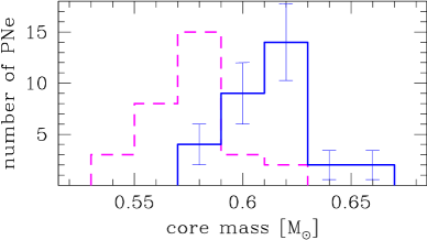
Figure 5: The masses of the PN central stars for the 31 objects studied here with HST and VLT data. The solid (blue) line shows the data obtained from equation 2; the dashed (magenta) line presents the masses obtained from accelerated post-AGB evolution (see further in the text). One-sigma errors are indicated.

This histogram shows that the proposed acceleration of post-AGB evolution can produce cspn masses in a good agreement with white dwarf masses: the peak of the mass distribution has shifted from 0.62 to 0.58 $M_{\sun}$. In addition, the accelerated tracks yield some masses as low as those obtained from pulsating PG1159.

Applying the same acceleration factor for all masses is the simplest adjustment possible. There are too few data points to search for more complex dependencies. The acceleration dependence on stellar mass and envelope mass should be verified with evolutionary codes, but this is beyond the scope of this paper.

4 Stellar initial masses and ages

The masses derived above refer to the final (white dwarf) mass of the evolving star. It is a challenge to relate this final mass to the initial mass of the progenitor star. The IFMR depends on the mass loss on the giant branches (McDonald et al., 2011). The model relations are very sensitive to the way mass loss is treated on the AGB and RGB. Theoretical isochrones incorporate different mass-loss assumptions and predict very different final masses. The IFMR is best calibrated for the lowest-mass stars using globular clusters and for intermediate mass stars using white dwarfs in open clusters. Both populations have different metallicities so their IFMR might differ (see Fig. 13 below). In between the two populations, the relation is also quite uncertain.

Here we use theoretical isochrones and empirical cluster white-dwarf masses to relate our final masses to progenitor masses. Given the uncertainties involved, the resulting mass should be seen as indicative only.

Having estimated the initial masses, we can later relate them to the total stellar ages, since the ZAMS. This relation is much better known, as discussed further in the text, and these ages are compared later with the Galactic bulge age.

4.1 Empirical initial–final mass relations

Empirical relations have been determined using white dwarfs in open clusters, which combine spectroscopic masses, model cooling ages, and cluster ages. We have used the data from Casewell et al., (2009), and references therein, as supplemented with recent data from McDonald et al., (2011) and Dobbie et al., (2012), to calculate an average white dwarf mass and initial mass per cluster. For each cluster, we left out white dwarfs with significantly higher masses than the minimum white dwarf masses to avoid cooling age uncertainties. The resulting data are listed in Table 3 and plotted in Fig. 6. For the initial mass, we used a minimum uncertainty of 0.2 $M_{\sun}$, or 0.1 $M_{\sun}$ for masses of $\lesssim 2\,M_{\sun}$ (apart for omega Cen); otherwise the uncertainties are estimated from the scatter between individual stars in the cluster.

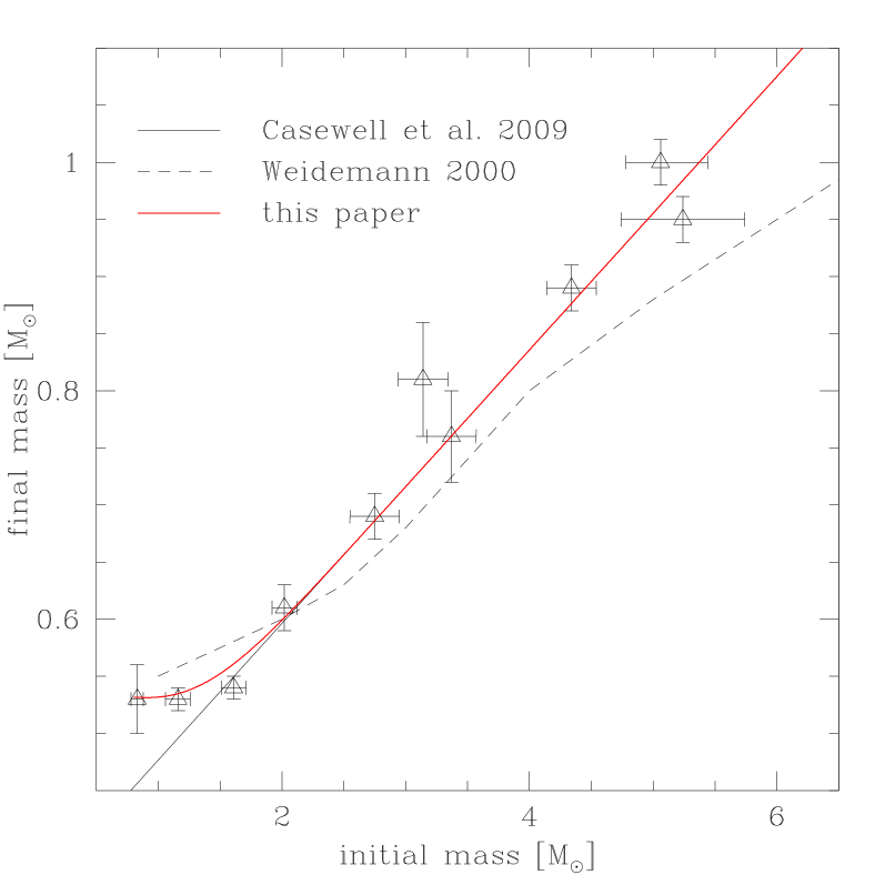
Figure 6: Initial-final masses for stellar clusters. For each cluster, an average initial and final mass are shown, based on data from Casewell et al., (2009) and references therein. For NGC2516 we used Dobbie et al., (2012), and we also included the globular cluster omega Cen (McDonald et al., 2011). The drawn line gives the linear fit of Casewell et al, whilst the dashed line is the older relation of Weidemann, (2000). The red line shows the relation derived here, Eq. (12).

The initial-final relation is well represented by the linear relation of Casewell et al., (2009) at higher initial masses, but this relation undershoots for the lowest masses (where the older Weidemann, (2000) relation is higher). The closest initial mass to the Sun is provided by the cluster NGC6791, where white dwarf masses are around 0.53 $M_{\sun}$. For omega Cen, 0.8 $M_{\sun}$ progenitors have evolved into 0.53 $M_{\sun}$ white dwarfs (McDonald et al., 2011) (where the lower metallicity of omega Cen should be considered; however, solar metallicity stars of this mass are longer lived and have not yet formed white dwarfs). The Casewell relation predicts white dwarf masses in globular clusters well below 0.5 $M_{\sun}$, which would require helium white dwarfs. Instead, the presence of AGB stars in globular clusters shows that they do yield some C/O white dwarfs. The Casewell relation therefore seems too low for the lowest initial masses.

To better fit the empirical relation, we add a term to the Casewell relation:

$$M_{\rm f}=0.3569+0.1197\times M_{\rm i}+0.15\times\exp[-(M_{\rm i})^{2}]\ {M_{\sun}}$$ (12)

(valid for $(M_{\rm i}>0.8\,M_{\sun}$). This relation is shown by the red line in Fig. 6. It removes the mismatch at the lowest masses.

Table 3: Average initial and final masses from cluster white dwarfs, based on data in Casewell et al., (2009); McDonald et al., (2011); Dobbie et al., (2012). Minimum uncertainties on the initial mass are taken as 0.2 $M_{\sun}$ or 0.1 $M_{\sun}$ for masses of $\lesssim 2\,M_{\sun}$ (apart for omega Cen); otherwise, the uncertainties are estimated from the scatter between individual stars in the cluster.

cluster	$M_{\rm f}$	$\delta M_{\rm f}$	$M_{\rm i}$	$\delta M_{\rm i}$
N6819	0.54	0.01	1.61	+0.1 $-$0.1
N7789	0.61	0.02	2.02	+0.1 $-$0.1
N6791	0.53	0.01	1.16	+0.1 $-$0.1
N2168	0.89	0.02	4.34	+0.2 $-$0.2
N2516	0.95	0.02	5.24	+0.5 $-$0.5
N6633	0.81	0.05	3.14	+0.2 $-$0.2
Sirius B	1.00	0.02	5.06	+0.4 $-$0.3
Praesepe	0.76	0.04	3.37	+0.2 $-$0.2
Hyades	0.69	0.02	2.75	+0.2 $-$0.2
Omega Cen	0.53	0.03	0.83	+0.05 $-$0.05

4.2 Stellar life times

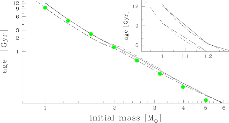
Figure 7: The initial mass vs. the age from the ZAMS to the end of the AGB for the Weiss & Ferguson, (2009) model at $Z=0.02$ (drawn line) and $Z=0.008$ (dashed line) and for the Padova isochrones at $Z=0.019$ and $Z=0.008$ (dot-dashed and dotted lines). The large (green) dots indicate the approximated relation.

In Fig. 7, we plot the stellar life times from the ZAMS until the end of the TP-AGB versus the initial stellar mass. The curves are taken from Weiss & Ferguson, (2009) for $Z=0.02$ and $Z=0.008$ (drawn and dashed lines) and from Girardi et al., (2000) for $Z=0.019$ and $Z=0.008$ (dot-dashed and dotted lines). There is better agreement between different models than for the IFMR discussed above. The insert shows the area of our interest on a linear scale.

In the following analysis, we use the linear (in the log–log plane) relation shown by filled circles in Fig. 7 which is defined as

$$\log({\rm age})=9.98-2.95\times\log({\rm initial\leavevmode\nobreak\ mass}).$$ (13)

This is our approximation to the set of fairly similar theoretical dependencies. These model relations show a small deviation near ZAMS mass of 1.8 M_☉: our straight line was chosen to better approximate the low-mass regime (between 1 and 2 M_☉) and misses the better defined high mass end. Tests have shown that different choices for the fitted line, if restricted to the range covered by different model relations, have only a small effect on the derived ages.

4.3 ZAMS masses and ages

Figure 8: The histograms of the interpolated data. The left panel shows the “accelerated” cspn masses; the central panel shows the initial ZAMS masses from empirical IFMR, and the right panel shows the ages since the ZAMS.

To derive stellar ages, we follow the procedure derived above. From the kinematical models we derive a nebular age and stellar temperature. This parameter pair is fitted to a post-AGB stellar evolution model, which yields (the “accelerated” case) a core mass through Eq. (11). The initial mass is derived using an IFMR defined by Eq. 12. Finally, the stellar age is derived from the mass, and from the condition that the star is in the post-AGB phase evolution, what means that it has finished its main sequence and giant branches evolution (Eq. (13) and Fig. 7). The stellar age is called the ‘total age’ or ‘age since ZAMS’ to distinguish it from the earlier derived kinematical age of the nebula.

In Fig. 8, we show the results of our interpolation routines in the form of histograms. The left-most panel shows the final masses derived from our interpolation routines; the central panel shows initial ZAMS masses, and the right panel shows the total ages of the stars.

The derived stellar ages are surprisingly low. The peak corresponds to ages as young as 1–2 Gyr. Without the derived acceleration of the post-AGB tracks, the ages would be even lower. These ages should be compared to what is known about the stellar populations for the bulge.

4.4 The age of the bulge

Age determinations of the GB are mostly based on comparison between observed and computed colour-magnitude diagrams. Different observations and computed isochrones generally agree and indicate that the stars in the GB are about 8–10 Gyr (Vanhollebeke et al., 2009) or 10–12 Gyr (Zoccali, 2009) old. These are about 2 Gyr younger than the oldest stellar populations of the Milky Way (McWilliam & Zoccali, 2010).

There is evidence that there is also a younger population towards the bulge. The VLT/MAD observations of the globular cluster Terzan 5, which are located near the Galactic centre, show the existence of two horizontal branches. These are interpreted as two populations (comparable in number) that differ in metallicities by a factor of 3 and with ages of 6 and 12 Gyr (Ferraro et al., 2009). They suggest a relation to a disruption of a dwarf galaxy that contributed to the formation of the Galactic bulge.

A younger bulge population has been found by Bensby et al., (2010, 2011, 2013) as mentioned in the Introduction. Uttenthaler et al., (2007) find evidence of the third dredge-up in four out of 27 bulge AGB stars based on the presence of radioactive technetium. The third dredge-up is not expected to operate in 1 $M_{\sun}$ stars and requires a younger population. Finally, Nataf et al., (2010) derive an enhanced helium enrichment from the red giant branch bump of the GB. They state that if confirmed this would lead to a downward revision of the 10+ Gyr age of the GB. These results indicate that younger stars are a minor component of the bulge. The dominant population is older with ages $>5$ Gyr.

Another uncertainty is the duration of the star-formation episode (Nataf & Gould, 2012). The assumption of rapid gravitational infall yields a bulge formation time of about 0.5 Gyr. The assumption that the bulge is formed from accreted stellar clumps gives a bulge formation time of 2.0 Gyr. However, star counts and radial velocities find that bulge kinematics are consistent with a pure N-body bar that evolved from secular instabilities, which would imply that bulge stars are just disk stars on bar orbits and would suggest a duration of star-formation with a time frame as extended as that of the inner disk.

This information on the bulge age(s) imposes strong constraints on the ages of central stars of GB PNe and suggests ages older than those shown in Fig. 8. This can be accommodated by using the IFMR as a free parameter.

5 The PN population of the Galactic bulge

Before concluding on the IFMR, we need to discuss whether our sample can be compared with the dominant GB population and search for possible factors disturbing the derived histograms.

5.1 Birth rate of planetary nebulae in the bulge

To interpret the results above in terms of bulge evolution, we first need to show that planetary nebulae trace the bulge population and that our selected objects are representative.

The mass-loss event, which ejects the planetary nebulae occurs for all low and intermediate-mass stars. The mass is ejected while the star is evolving up the asymptotic giant branch, and is ionized while evolving towards the white dwarf phase. The lowest- and highest-mass stars may avoid visibility as a PN (Low mass stars evolve so slowly that the ejecta have dispersed before the star can ionize them, which is the so-called “lazy PN”, while high-mass stars evolve too fast and only emit high levels of ionizing radiation for a brief period.), but apart from this, all stars are expected to be surrounded by a detectable PN for a significant length of time.

Evidence that the oldest stellar populations suffer from the “lazy PN” process comes from globular clusters, where there are fewer PNe detected than expected based on the number of stars (Jacoby et al., 1997). In contrast, PNe are not rare in the bulge: about a quarter of known Galactic PNe are located towards the Galactic bulge. This already suggests that the bulge population, either in part or in its entirety, is not as old as the globular clusters.

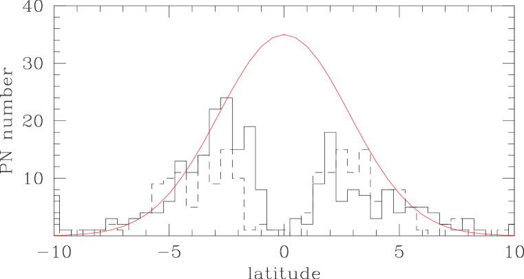
Figure 9: The galactic latitude ($b$) distribution of PNe between 0 and 4 degree longitude (solid line) and between 356 and 0 degree longitude (dashed line), as fitted with a Gaussian of form $\exp(-b^{2}/4^{2})$.

To quantify the bulge PN population, there are currently 785 PNe catalogued in the direction of the Galactic bulge, which have a Galactic latitude and longitude within 10 degrees of the Galactic Centre (Acker et al., 1992; Parker et al., 2006; Miszalski et al., 2008). The distribution is patchy and due to the high extinction, none are seen within a degree of the Galactic plane. Figure 9 shows the latitude distribution of PNe within $0^{\circ}<l<4^{\circ}$. The distribution is fitted with a Gaussian. Integrating under the Gaussian indicates that half the objects are missing. The deficit is a bit larger at negative longitudes. Correcting the known number of PNe for this deficit suggests that approximately 2000 PNe are present in the bulge.

We can convert this to a birth rate if we know the visibility time. Most known PNe in the bulge are intrinsically bright: faint nebulae have been difficult to detect against the crowded stellar background. The brightest phase of a PN ends when either the nebula becomes optically thin to ionizing radiation or the star leaves the horizontal evolutionary track and enters the white dwarf cooling track. This happens after $\sim 5000$ yr (see Blöcker, (1995)). Gesicki et al., (2006) find that bulge PNe tend to have kinematic ages less than 6000 yr. Combining this observational life time of 6000 yr with the predicted number of 2000, such PNe, gives an indicative PN birth rate in the bulge of $\sim 0.3\,\rm yr^{-1}$.

Figure 10: For an assumed original stellar mass of $10^{10}$ $M_{\sun}$ formed in a burst, the plot shows the stellar death rate (number of stars leaving the AGB per year) as a function of age since the star burst. The top panel shows the corresponding main-sequence turn-off mass.

The rate at which stars leave the AGB (the stellar death rate) can be calculated for a single age (star burst) stellar population. We use the models of Maraston, (1998), which are based on the FRANEC isochrones, for solar metallicity to find the change in turn-off mass per year and relate this to a number of stars by assuming a Salpeter initial mass function starting from 0.25 $M_{\sun}$. For a total original stellar mass in the bulge of $10^{10}\,M_{\sun}$ (McGaugh, 2008; Flynn et al., 2006), the stellar death rate as function of age of the burst is shown in Fig. 10. The death rate is almost independent of age if the burst is older than 7 Gyr at around 0.6–0.4 stars per year.

There is good consistency (within a factor 1.5–2) between the PN birth rate and the stellar death rate for a $10^{10}\,M_{\sun}$ bulge population for a stellar age $>7\,$Gyr. For younger populations, the PN birth rate is a factor of 2 or more below. Planetary nebulae therefore trace a significant stellar population of the bulge with some bias towards the younger stars. If the bulge is entirely old, the birth and death rates imply that most bulge stars produce visible PNe: this would put limits on any very old population ($>10^{10}\,$yr), which would be deficient in PNe (see section 5.2). If there is a younger population in the bulge, this would dominate the PN population as long as this younger population is large enough (of order 10–50% depending on age).

5.2 PN visibility

The most uncertain part of this calculation is the visibility time. Predicted PNe numbers in the Solar neighbourhood suggest visibility times of 25 000 – 50 000 years (Zijlstra & Pottasch, 1991; Moe & De Marco, 2006) (the latter predict 3600 PNe within the bulge). Our assumed visibility time for bulge PNe is much less because the crowded stellar field combined with the relatively low angular resolution of the original discovery plates renders faint extended nebulae as poorly detectable. Our visibility time assumes that the observed bulge population is dominated by bright, compact PNe with central stars on the horizontal part of the track (prior to their initial rapid fading when entering the cooling track) and dense, optically thick nebulae.

The models of Schönberner et al., (2007) show that the majority of PNe on the horizontal part are expected to be optically thin and therefore, are already decreasing in nebular luminosity. However, the spectra for our sample of the bulge PNe show evidence for low ionization lines, such as [O i], for 24 out of 31 objects, which indicates that these must be optically thick in some directions (see also Guzman-Ramirez et al., 2011). This discrepancy between the models and data may be explained by asphericities. Our spectra were taken mostly along the minor axis where the highest densities are found. An ionization front may be trapped along the minor axis, whilst the polar directions are already optically thin. However, optically thin nebulae show only moderate fading before rapid fading on the cooling track (Schönberner et al., 2007), so this issue should not affect the visibility time significantly.

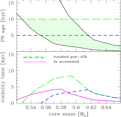
Figure 11: The top panel shows the kinematic (nebular) ages derived from the interpolated Blöcker tracks (without the 0.546 $M_{\sun}$ model) for the point (i) when the star reaches 20 kK (lower solid line) and (ii) when the star has faded by a factor of 10 in luminosity (upper solid line). The dashed lines show the 10 kyr age when the nebula is assumed to become optically thin, and the 5 kyr age corresponds to the size limit of the HST-selected sample of 5 arcsec. The hashed area defines the visibility time of a bright PN.
The lower panel shows the corresponding visibility time. The long-dashed (green) line shows the visibility time for the 10 kyr limit. The dashed (blue) line shows the visibility time for the HST-selected sample (5 kyr limit). The solid line shows the same but for the accelerated tracks.

Because PNe trace the dominant bulge populations, there is no implication that they trace all populations equally. If we take a limiting radius of 0.2 pc for a bright PN (10 arcsec diameter at the distance of the bulge, which is twice the limit of our survey), this corresponds to an expansion age of 10 000 yr for an expansion velocity of 20 km s^-1) or 5 000 yr for 40 km s^-1. The higher value is found in models (Schönberner et al. 2005); our data shows about equal numbers of lower and higher velocities, correcting for the outer edge, which expands 1.4 times faster than the mass-averaged velocity derived from the spectra. A PN becomes observable once the central star reaches a temperature of 20 kK and fades when either the nebula becomes optically thin to ionizing radiation or the star begins to fade.

We define the end of the visibility time as the moment when the stellar luminosity has declined by a factor of 10, or the nebula has reached an age of 10 kyr, whichever occurs sooner. For the newly interpolated Blöcker tracks, we plot these times in Fig. 11, top panel. The hashed region indicates when a bright PN is visible, according to this criterion. The lower panel shows the corresponding visibility time for both the interpolated and the accelerated Blöcker tracks.

Above 0.61 $M_{\sun}$ (0.58 for the accelerated tracks), the visibility time is limited by the fading of the star and shortens rapidly at higher masses. Below 0.56 $M_{\sun}$, the nebula is already older than 5000 yr by the time ionization starts, and this reduces the visibility time. For the accelerated tracks, these limits are 0.58 $M_{\sun}$ and 0.52 $M_{\sun}$, respectively. The bright PN population will be dominated by the stars with core masses in the range 0.56–0.61 $M_{\sun}$ (0.52–0.58 $M_{\sun}$ for the accelerated tracks), where the visibility time is maximum. If much fainter PNe are considered, the mass limits become relaxed.

More accurate visibility times can be found from the work of Schönberner et al., (2007), where several evolutionary sequences of model PNe were presented and computed with a 1-D radiation-hydrodynamic code. They calculate total line fluxes as function of time. For the [O iii] flux, the visibility times at $M(5007)<-1$ are shown in Fig. 15 of Schönberner et al., (2007). A similar result would be obtained for H$\beta$. We note that these are optically thin models, which expand faster than the value of 20 km s^-1 assumed above; the transition times are also included. From their figures, it can be clearly seen that if the faint limit is relaxed to $M=0$, the visibility times of the faint models increase significantly. If relaxed further to $M>1$, the more massive stars contribute for long periods of time. This confirms how sensitive the life times (and therefore number densities) are to the survey flux limits.

The observed H$\beta$ line flux for our HST bulge sample varies between $-11.9$ and $-14.2$ in units of ergs cm^-2 s^-1 (or mW m^-2). After correcting for extinction, the range is between $-10.0$ and $-12.7$, which spans a range of 2.7 dex. However, the large majority fall within a range of a factor of 10 from $-10.5$ to $-11.5$, which is consistent with the assumption that the known bulge population is significantly flux limited.

5.3 Selection bias

The discussion in the previous subsection shows that the relation between the PNe and the underlying stellar population depends on how the sample is selected. A bright sample is biassed towards lower core masses, while a fainter sample is sensitive to higher core masses - a somewhat counter-intuitive effect.

The selection effects are more complex. The presence in the PN catalogues mainly depends on the [O iii] fluxes, which depends on stellar luminosity, size, and density of the nebula and foreground extinction. In dense star fields, there may be a bias against highly extended objects. High-resolution spectroscopy requires a high surface brightness due to the narrow slits. The surface brightness declines as $\sim r^{-3}$–$r^{-3.5}$ (Frew & Parker 2006) for nebulae larger than 0.1pc in radius. This declines introduces a bias against extended objects.

The HST sample was selected as an unbiased survey of compact PNe and was taken from a random selection of nebulae of less than 5 arcsec diameter (0.2 pc at the distance of the bulge). There is no flux limit imposed other than those in the original PNe surveys. Selecting compact nebulae negates the problem caused by decreasing surface brightness of larger nebulae. Echelle spectra were obtained for all objects observed by HST, which are independent of brightness, thus removing a second potential bias. The size limit corresponds to an age of 2 500–5 000 yr, depending on assumed expansion velocity ($V_{\rm aver}=15$–30 km s^-1: Table 1). The corresponding visibility curves are shown in Fig. 11. The visibility time for inclusion in the sample is shown by the dashed line in the bottom panel. Compared to the original curve, the distribution of visibility time versus core mass is much more uniform, which varies by no more than a factor of two over the range of masses considered here (depicted is a wider range). The visibility time for a core mass of 0.696 $M_{\sun}$ (not shown) is down by a factor of four compared to the peak at about 0.62 $M_{\sun}$ and is about 830 yr.

For the accelerated tracks, the visibility time increases at lower masses and decreases at higher masses; it varies only by about a factor four over the considered range. Even for these models, the HST sample is less biased than other samples currently available and is sensitive to a wide range of core masses, but stars at the lowest and highest core masses may still be under-represented. The derived ages distribution of PN central stars can be corrected for this bias.

5.4 Constraints by chemical composition

Figure 12: The distribution of oxygen abundance within our sample. The data taken from Table 1 are presented relative to solar value (8.69 adopted from Asplund et al., (2009)).

Ness et al., (2013) recently analysed the metallicity of the GB. The sample of 28 000 stars allowed them to define a number of subsets with different [Fe/H] values. The three dominant components (named A, B, and C in their plots and tables) cover the range of [Fe/H] between $-1.0$ and +0.5. We do not have iron abundance data, but we show the oxygen data instead in Fig. 12, which is presented relative to the solar abundance so it can be compared directly to the plots of Ness et al., (2013). Our sample shows the same trend by indicating a slightly sub-solar metallicity in general. Scarcity of data does not allow for more detailed comparison; however, these data do not contradict our previous statement (see Sect. 5.1) that our sample corresponds to the dominant GB population.

6 The star-formation history of the bulge

Knowing that the best approximation to the empirical IFMR resulted in total ages that are too young we use the IFMR as a free parameter and adjust it trying to achieve better agreement. An alternative would be to apply a further adjustment to the Blöcker model: either of these possibilities can increase the ages.

6.1 Model initial-final mass relations

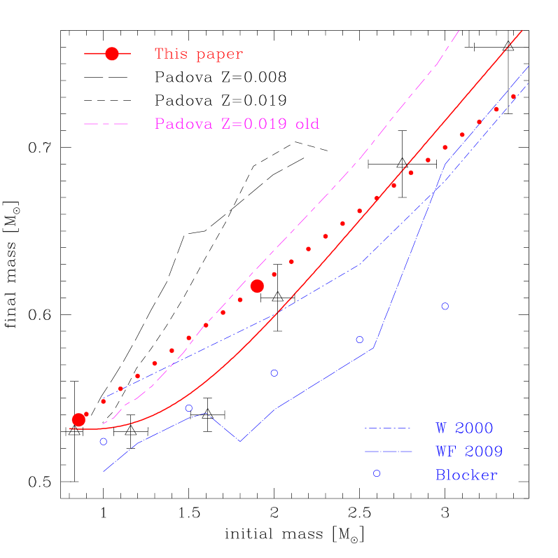
Figure 13: The initial vs. final mass relation plotted for several models: Padova tracks (two sets at solar and one at subsolar metallicity); Weidemann, (2000); Weiss & Ferguson, (2009) (solar metallicity). The open circles follow the IFMR interpolated from Blöcker, (1995). The solid line follows IFMR as defined by Eq. (12); the filled dots correspond to the best-fit IFMR described in the text.

In Fig. 13, the empirical relations are compared to those obtained from evolutionary models. From the “Padova database of stellar evolutionary tracks and isochrones”, we show (long-short-dash magenta line) the set from Girardi et al., (2000) (with a simplified thermal-pulsing AGB treatment). For solar metallicity we also show a more recent set from Marigo et al., (2008) (with a state-of-the-art description of the thermal-pulsing AGB phase), which predicts a steeper IFMR (the higher short-dash black line). At lower metallicity, the relation is even steeper (long-dashed black line). Generally the new data show larger scatter with no unambiguous IFMR. The Padova isochrones are being improved and extended (Bressan et al., 2012), however for the moment; the isochrones do not include the TP-AGB. Weiss & Ferguson, (2009) have also published a grid of stellar models for stars on the AGB and post-AGB. Their data also show significant scatter below initial masses of 2 $M_{\sun}$.

Comparing these relations to the empirical IFMR above, the agreement is poor. The old Padova set lies above the Casewell relation by some 0.05 $M_{\sun}$. The new set lies even higher. The Blöcker IFMR, in contrast, lies well below the empirical relation, and the Weiss & Ferguson, (2009) models are even lower. The Weidemann, (2000) relation still provides a better match than any of these models.

In the models, the final masses are largely determined by the mass-loss prescription. The Weiss & Ferguson, (2009) models show low core masses due to the use of the Wachter et al. (2002) formalism leading to higher mass-loss rates. We still lack a formalism, which reproduces the IFMR measured in stellar clusters, and the scatter between the models (and data) is not a surprise.

6.2 Adjusting the IFMR to fit bulge ages

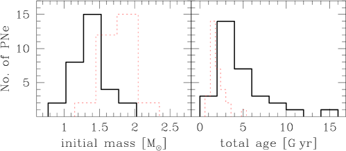
Figure 14: The histograms of the interpolated data. The left panel shows the initial ZAMS masses, and the right panel shows the ages since the ZAMS was used later to derive a star-formation history (see Fig. 15). The solid lines represent the data obtained with IFMR defined by Eq. (14), while the thin dotted (red) lines repeat the histograms from Fig. 8 for comparison.

From a selection of published ages of GB discussed in Sect. 4.4, we focus on the data of Bensby et al., (2013). They have the advantage that they are based on a detailed and homogeneous analysis of 58 individual stars; the data are presented in the tables, can be grouped according to metallicity, and visualized as histograms. Most other data comes from isochrones fitted to colour–magnitude diagrams.

The cspn “accelerated” masses obtained in Sect. 3 should be mapped to the desired age distribution with the use of an appropriate IFMR. From Fig. 13, it can be seen that the situation is complicated, and using a relation of higher order than linear is not justified.

We anchor the linear IFMR to the youngest and oldest objects from the sample of Bensby et al., (2013), which is up to about 1.6 and 14.7 Gyr. These should correspond to our most- and least-massive cspn. Applying the relation for age–mass (Eq. (13)), we obtain an initial mass of 1.90 $M_{\sun}$ and age $1.4\times 10^{9}$ yrs for the youngest object (that of final mass of 0.617 $M_{\sun}$), while obtaining an initial mass of 0.855 $M_{\sun}$ and age $14.0\times 10^{9}$ yrs for the oldest (having final mass of 0.537 $M_{\sun}$). These two points are shown as large dots in Fig. 13, while small dots follow the proposed linear approximation to the IFMR:

$$M_{\rm i}=(M_{\rm f}-0.472)/0.076.$$ (14)

This relation was used to convert our final masses into total ages. The results are shown in Fig. 14. The solid line represents the data obtained with IFMR defined by Eq. (14). For a comparison, these are overplotted (with a thin dotted red line) with the histograms from Fig. 8 obtained previously with the IFMR defined by Eq. (12). We see now that the ages correspond far better to what is expected for the bulge objects.

The large discrepancies between the various model IFMRs and the cluster IFMR remain a concern. It would help this research if the IFMR were better established. We also note that our choice to adjust the IFMR is non-unique. A higher acceleration of the Blöcker tracks could also increase the ages, and with a known IFMR, it would be possible to constrain the post-AGB evolution.

6.3 The star-formation history of the bulge from PNe

To obtain the star-formation history from the age distribution, we need to correct for observational biases. The number of objects is corrected for the difference in visibility time as a function of core mass (see the discussion in Sect. 5.3) using the relation for the accelerated tracks. The visibility correction reduces the peak and raises the wings of the distribution. Finally, the curves are divided by the PN birth rate (stellar death rate) as function of stellar age (Fig. 10). This correction reduces the star-formation rates for younger populations (which produce more PNe per unit mass). The correction becomes negligible for ages more than 7 Gyr, but is large for ages less than 4 Gyr.

The resulting histogram of the star-formation rate, normalized to unity, is shown in Fig. 15 as a solid line. It is derived from the right panel of Fig. 14. The applied corrections flatten the peak near 3 Gyr and elevate the single oldest object.

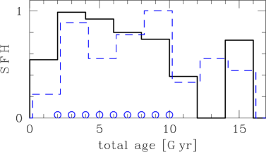
Figure 15: The star-formation history for the Galactic bulge derived from the right panel of Fig. 14, which is corrected for visibility time and PNe birth rate. A dashed (blue) line, which is slightly shifted for a better presentation, shows the overplotted histogram from Bensby et al., (2013) for the bulge stars, excluding the most metal-poor objects. The open circles represent the points at which a constant SFH was backward-corrected for visibility time and PNe birth rate, as shown in Fig. 16.

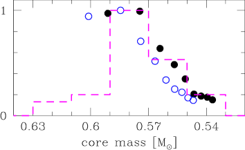
Figure 16: The open circles show the core-mass distribution (normalized to unity) obtained from a constant SFH, which was backward-corrected for visibility time and for the PNe birth rate at the points indicated in Fig. 15. The mass-axis is drawn in reverse order to allow a direct correspondence of the large dots from left to right in both figures. For comparison the dashed line shows the final mass distribution repeated from Fig. 5. The filled circles represent the same data points as open circles but obtained with modified IFMR defined by Eq. 15.

Bensby et al., (2013) find that the age distributions for their stars change with metallicity with the stars with solar and higher metallicity being predominantly of intermediate age, and the metal-poor populations peaking at ages older than 10 Gyr. The detailed results in the publication allows us to compare our histogram with different subsets of Bensby et al., (2013). Our result agrees best with their “regular-metallicity” sample ($-0.5<[{\rm Fe/H}]<+0.6$), which we obtained by excluding the 15 most metal-poor ($[{\rm Fe/H}]\leq-0.5$) stars from the whole sample. This distribution (normalized to unity) is overplotted on our histogram in Fig. 15 as the dashed (green) line. By considering all uncertainties that concern post-AGB evolution and IFMR, the similarity in shape of both dependencies seems remarkable.

The older, metal-poor population is much less apparent in our data. This can be interpreted as a selection bias in that the lowest-mass (oldest) stars may be lacking in the sample of compact PNe for reasons discussed before. The abundance study of Chiappini et al., (2009) shows that bulge PNe have metallicities that range from solar-like to about $-0.5$dex with few if any lower metallicity objects. Therefore, the lower metallicity population in the bulge indeed appears to have produced a few bright PNe. A deep survey for faint PNe may find a missing low-metallicity, old-progenitor population.

To verify the method, we tried to invert the correction routines and apply them to the SFH that follows from Bensby et al., (2013). Figure 15 shows that the SFR can be crudely approximated as a constant over the range 2–10 Gyr. If everything is correct we should obtain a distribution similar to the cspn masses shown in Fig. 5. Figure 16 shows this result. The open circles correspond to those of Fig. 15, and because equally spaced total ages do not correspond to equally spaced cspn masses, we made these dots denser than the histogram bins. The dashed (magenta) line is copied from Fig. 5. The similarity is obvious. We are tempted to search for an IFMR that improves the fit. The result is shown with filled circles. Equation 14 needs only a slight modification by adding 0.01

$$M_{\rm i}=(M_{\rm f}-0.472+0.01)/0.076.$$ (15)

This modification shifts cspn (final) masses towards lower values, and if the new relation was drawn in Fig. 13, it would be shifted downwards from the old dotted line, which shift is not much more than the diameter of the big circles. This is much smaller than the scatter between different IFMR. Apart from the IFMR, the mass-age relation is also involved (as a linear approximation), and it is very likely that both are not single relations of fixed metallicity. Applied here were also the visibility corrections for which we have only estimations. Therefore, we did not go further into fine-tuning of all these relations. We can conclude that the proposed IFMR fits reasonably and consistently to our data and to Bensby et al., (2013) within an accuracy of about $0.01\,M_{\sun}$ for the final masses.

7 Conclusions

The purpose of the investigation is to use the masses and ages of the central stars of planetary nebulae to constrain their evolution and to derive a star-formation history of the Galactic bulge. Our conclusions are as follows:

• We use HST images and VLT echelle spectra of 31 compact bulge planetary nebulae to derive expansion ages for the nebulae. The Torun models are used to calculate the mass-averaged expansion velocities. A correction factor is derived from published hydrodynamical models (Perinotto et al., 2004) to relate this to the expansion of the outer radius. The expansion age of the nebula and the temperature of the central star are fitted to post-AGB model tracks to derive masses of the central stars.

• We use the set of Blöcker post-AGB tracks. Two problems are identified with these tracks: the extremely slow evolution of the lowest mass tracks prohibits the formation of an ionized planetary nebula, and the final stellar masses are higher than white dwarf masses and asteroseismology masses. To force consistency, we exclude the lowest mass model from the model interpolations. We also make the ad-hoc adjustment that the envelope masses could be overestimated to accelerate the Blöcker tracks by a constant factor of three. This produces consistency with white dwarf masses and allows for the lowest masses of PN central stars found from asteroseismology. We note that the white dwarf mass distribution in the bulge is not known and that the acceleration proposed as constant can actually depend on stellar mass and envelope mass.

• An IFMR is applied to the central star masses to derive the original (ZAMS) masses. An observational relation is derived from white dwarf masses in clusters. This gives a relation in very good agreement with Casewell et al., (2009) but with a shallowing at the lowest masses to allow for 0.53 $M_{\sun}$ white dwarf masses in globular clusters. A simple relation is proposed to estimate the total ages of the stars.

• The derived ages are lower than seems plausible for bulge populations. To improve the agreement between the derived ages and the published data on Galactic bulge ages, we use the IFMR as a free parameter and adjust it to a linear IFMR that relates our youngest and oldest object with corresponding youngest and oldest bulge stars in Bensby et al., (2013). Such an IFMR appears steeper than other observational relations but is not as steep as some assumed for evolutionary calculations. With this IFMR, the total ages of our bulge objects cover the desired range. A further acceleration of the Blöcker tracks is a possible alternative to adjusting IFMR.

• To convert the age distribution of the PN central stars to a star-formation history, the inherent bias needs to be quantified. We estimate the total number of PNe present in the bulge as 2000. We calculate the visibility time as a compact PN as a function of final mass and the stellar death rate (or PN birth rate) as function of age of the stellar population. The age distribution is corrected for these functions. After the correction an apparent peak at 3 Gyr disappears, which confirms the role of observational bias.

• The age distribution obtained by us is consistent with the subsample of Bensby et al., (2013) with metallicities close to solar values. The derived star-formation history shows a constant rate over time in general.

• The set of proposed procedures was eventually verified by applying it in an inverted version to the final, approximately constant SFH. This resulted (as expected) in a core-mass distribution similar to the one obtained from PNe with an accuracy of about $0.01\,M_{\sun}$. The derived masses, ages and relations compose a rather consistent picture.

• Our results agree with an extended star formation in the Galactic bulge, which was approximately constant between 3 and 10 Gyr ago. This is more consistent with a secular development of the bulge, as expected from interaction with a bar. There may still be an older component of the bulge with a different origin, as the metal-poor population in the bulge region seems to be poorly represented among the compact PNe.

Appendix A The observations and models of planetary nebulae

The model fitting procedure was described in brief in Sect. 2.3. A full description can be found in Gesicki et al., (2006), where we applied a genetic algorithm for the first time to locate the best fit parameters.

We searched for the density and velocity distributions as simply as possible. The density was assumed similar to a reversed parabola with both edges modified to fit the images. The best fit was judged by visual inspection of the superposed images shown below in the boxes marked “surface brightness”. The stellar temperature, luminosity, and the ionized mass was derived by PIKAIA as a compromise to a simultaneously satisfying fit to all available emission strengths (see Table LABEL:pne_ratios). The density values at the innermost and outermost edges were additionally modified to reproduce the strengths of emissions originated there, but the velocity field was solely derived by the PIKAIA routine, which judges the results by the quality of emission profile fitting (least squares method). The best velocity field was searched among linear or parabola shapes. More complicated velocity fields were not considered. Wherever the parabola provided no improvement of the fit, we adopted the linear velocity as the simplest.

This method was applied identically for all 31 objects presented below. The largest nebulae and those barely resolved are treated in the same way to allow us to discuss the whole data set consistently.

The series of figures (Figs. 17–47, one per object) present the HST observations with the derived model dependencies. The HST image are shown rotated, such that the VLT echelle spectroscopic slit is horizontal. In most cases, this puts the slit along the minor axis of the PN. The echelle spectrum was extracted from the central arcsecond only. For extended objects, outer areas of the slit were not used. Wherever no observational data was available, we left the corresponding box empty.

Table 4: Galactic bulge PNe observed H$\beta$ fluxes and line strengths together with the corresponding photoionization model results. The line strengths are normalized to the strengths of H$\beta$ equal 1. For each object, the first row contains the observed parameters while the corresponding model values are typed below (in the next line).

PN G	name	$\log F({\rm H}\beta)$	He ii	[N ii]	[O i]	[O ii]	[O iii]	[S ii]	[S iii]
			4686Å	6583Å	6302Å	3729Å	5007Å	6731Å	6312Å
001.7-04.4	H 1-55	-11.5	–	2.77E+00	2.00E-02	2.30E-01	1.10E-01	1.90E-01	2.90E-03
		-12.2	2.15E-05	3.49E+00	4.97E-03	2.72E-01	1.56E-01	1.77E-01	6.33E-03
002.3-03.4	H 2-37	-11.9	–	1.11E+00	1.59E-02	–	8.07E+00	8.00E-02	2.00E-02
		-11.5	2.78E-01	1.29E+00	1.35E-03	3.07E-01	6.51E+00	2.05E-02	1.82E-02
002.8+01.7	H 2-20	-11.0	–	2.81E+00	2.00E-02	9.90E-01	2.70E-01	1.10E-01	–
		-11.2	8.39E-06	3.12E+00	8.42E-03	5.72E-01	3.38E-01	5.30E-02	5.30E-02
002.9-03.9	H 2-39	-11.6	3.80E-01	5.80E-02	–	–	1.30E+01	1.29E-02	8.70E-03
		-11.5	4.43E-01	6.14E-02	3.01E-05	5.80E-02	1.09E+01	6.67E-04	2.48E-03
003.1+03.4	H 2-17	-11.3	–	1.91E+00	–	3.20E-01	1.00E-03	1.60E-01	–
		-11.7	5.49E-06	1.41E+00	3.23E-04	1.12E-01	4.12E-02	1.69E-01	1.86E-02
003.6+03.1	M 2-14	-11.4	2.40E-02	2.94E+00	2.20E-02	7.00E-01	2.36E+00	6.70E-02	1.30E-02
		-10.7	4.68E-04	2.49E+00	2.09E-03	1.61E-01	2.77E+00	2.71E-02	1.45E-02
003.8+05.3	H 2-15	-12.3	–	5.88E+00	1.20E-01	–	9.24E+00	4.00E-01	–
		-11.8	4.03E-02	2.96E+00	5.12E-02	1.11E+00	7.12E+00	1.27E-01	1.91E-02
004.1-03.8	KFL 11	-12.2	–	4.20E-01	–	–	8.65E+00	4.80E-02	–
		-11.0	5.59E-03	8.24E-01	1.07E-02	3.99E-01	6.34E+00	2.05E-02	7.82E-03
004.8+02.0	H 2-25	-11.2	–	9.50E-01	1.00E-02	1.50E+00	6.40E-01	3.00E-02	1.00E-02
		-11.1	1.13E-05	7.28E-01	5.85E-04	7.12E-01	5.90E-01	4.07E-02	1.08E-02
006.1+08.3	M 1-20	-10.8	–	4.50E-01	4.70E-02	5.50E-01	1.00E+01	2.30E-02	–
		-10.6	1.27E-02	3.67E-01	1.17E-02	1.55E-01	9.58E+00	1.17E-02	8.57E-03
006.3+04.4	H 2-18	-11.5	5.00E-02	7.80E-02	1.00E-02	1.60E-01	1.30E+01	1.80E-02	1.00E-02
		-11.0	7.80E-02	2.57E-03	5.58E-08	5.65E-03	7.80E+00	4.78E-06	2.22E-04
006.4+02.0	M 1-31	-10.0	–	1.39E+00	6.40E-02	3.30E-01	7.66E+00	6.90E-02	1.70E-02
		-9.51	1.84E-03	1.65E+00	6.33E-04	2.57E-02	4.20E+00	5.76E-03	1.16E-02
008.2+06.8	He 2-260	-11.7	–	9.10E-01	2.00E-02	1.54E+00	4.80E-02	4.00E-02	7.00E-03
		-11.0	8.80E-07	4.17E-01	1.90E-03	1.27E-01	3.75E-01	1.08E-02	7.46E-03
008.6-02.6	MaC 1-11	-11.2	–	8.10E-02	–	–	8.48E+00	–	–
		-11.1	3.39E-02	7.65E-02	5.64E-06	2.92E-02	8.75E+00	6.37E-04	2.60E-03
351.1+04.8	M 1-19	-10.8	–	8.20E-01	–	–	5.02E+00	3.90E-02	–
		-11.0	2.55E-03	8.92E-01	2.72E-03	3.64E-01	5.09E+00	3.48E-02	1.61E-02
351.9-01.9	Wray 16-286	-10.5	–	5.90E-01	–	–	1.06E+01	5.00E-02	–
		-10.5	5.37E-02	6.92E-01	2.53E-02	1.80E-01	1.27E+01	3.80E-02	1.16E-02
352.6+03.0	H 1-8	-10.5	–	2.50E+00	–	–	8.81E+00	9.70E-02	–
		-10.6	1.85E-02	1.55E+00	8.52E-03	1.49E-01	8.93E+00	3.19E-02	1.08E-02
354.5+03.3	Th 3-4	-10.6	–	9.20E-01	–	–	1.65E+01	–	–
		-10.5	1.41E-03	7.23E-01	1.39E-03	3.21E-02	4.56E+00	2.73E-03	1.04E-02
354.9+03.5	Th 3-6	-11.2	–	2.03E+00	–	–	2.09E+00	1.20E-01	–
		-11.0	3.85E-04	2.42E+00	3.16E-03	4.48E-01	2.18E+00	5.58E-02	9.04E-03
355.9+03.6	H 1-9	-10.6	–	6.30E-01	1.70E-02	–	1.89E+00	1.00E-02	2.30E-02
		-10.3	3.95E-05	5.74E-01	2.96E-03	2.50E-01	1.92E+00	1.55E-02	1.40E-02
356.1-03.3	H 2-26	-12.7	1.80E-01	6.21E+00	2.40E-01	–	6.28E+00	6.00E-01	–
		-12.0	4.14E-01	7.57E+00	1.24E-01	1.60E+00	6.31E+00	3.89E-01	3.89E-01
356.5-03.6	H 2-27	-11.9	–	1.58E+00	–	–	7.01E+00	1.90E-01	–
		-11.8	1.30E-02	3.07E+00	4.34E-02	1.11E+00	4.43E+00	1.29E-01	1.47E-02
356.8+03.3	Th 3-12	-11.8	–	3.05E+00	–	–	4.10E-01	1.20E-01	–
		-11.9	1.16E-05	2.96E+00	9.43E-03	3.32E-01	4.89E-01	1.03E-01	5.94E-03
356.9+04.4	M 3-38	-11.5	3.00E-01	1.47E+00	1.28E-01	–	1.53E+01	1.10E-01	4.70E-02
		-11.8	2.60E-01	1.68E+00	2.24E-03	1.04E-01	1.11E+01	1.70E-02	2.10E-02
357.1-04.7	H 1-43	-11.5	–	1.94E+00	1.40E-02	–	–	9.60E-02	–
		-12.1	2.18E-10	1.06E+00	3.31E-05	1.70E-02	1.38E-04	2.18E-01	1.54E-03
357.2+02.0	H 2-13	-10.9	–	6.60E-01	5.00E-02	–	1.55E+01	1.30E-01	1.70E-02
		-10.6	8.05E-02	1.31E+00	2.26E-02	3.52E-01	1.31E+01	4.39E-02	2.05E-02
358.5-04.2	H 1-46	-10.4	–	4.72E-01	2.00E-02	–	4.78E+00	2.41E-02	1.58E-02
		-10.2	5.11E-03	2.59E-01	4.07E-03	5.26E-02	6.63E+00	1.10E-02	1.37E-02
358.5+02.9	Al 2-F	-12.0	–	3.90E-02	–	–	1.39E+01	–	–
		-12.0	7.20E-01	3.88E-02	2.95E-06	2.65E-02	1.09E+01	1.77E-04	1.30E-03
358.7+05.2	M 3-40	-11.0	–	2.02E+00	–	–	–	1.30E-01	–
		-11.2	3.75E-03	2.36E+00	1.05E-02	4.58E-01	4.45E+00	6.18E-02	1.46E-02
358.9+03.4	H 1-19	-10.7	–	2.24E+00	–	–	3.98E+00	6.00E-02	–
		-10.9	8.99E-04	1.92E+00	2.50E-03	1.51E-01	2.93E+00	2.02E-02	9.40E-03
359.2+04.7	Th 3-14	-11.4	–	1.12E+00	–	6.30E-01	1.00E-02	1.60E-01	–
		-11.2	3.59E-09	2.15E+00	2.39E-03	1.12E-01	7.55E-04	1.04E-01	1.58E-03

Table 4: continued.

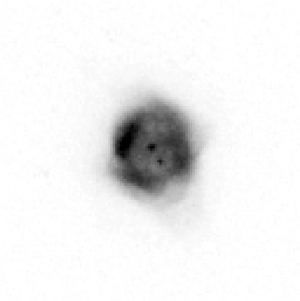
Figure 17: The nebula H 1-55 (PN G 001.7$-$04.4). The left panel shows the HST H$\alpha$ image in linear grey scale, which is rotated so that the VLT spectrograph slit runs horizontally through the centre. In the small panels, the observed data are drawn in solid lines (as a rule), while model fits and model parameters are in dotted and dashed lines. The “surface brightness” panel shows the horizontal slices through the H$\alpha$ and [O iii] image centre (averaged over nine pixels) with the model brightness profile superposed. Next, the radial distributions of the best-fit model for selected parameters are shown. The right-most panel shows the emission lines observed at the VLT with the superposed modelled line profiles corrected for instrumental broadening of 0.1Å.

Figure 25: The nebula H 2-25 (PN G 004.8+02.0). The data are presented as in Fig. 17.

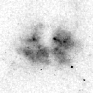
Figure 38: The nebula H 2-27 (PN G 356.5-03.6). The data are presented as in Fig. 17.

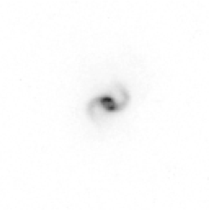
Figure 39: The nebula Th 3-12 (PN G 356.8+03.3). The data are presented as in Fig. 17. The very compact nebula shows a spiral-like structure, likely tracing a bipolar flow. The profiles do not show evidence for high-velocity flows and are well fitted.

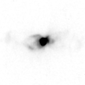
Figure 40: The nebula M 3-38 (PN G 356.9+04.4). The data are presented as in Fig. 17. The slit is oriented along the major axis.

Figure 41: The nebula H 1-43 (PN G 357.1-04.7). The data are presented as in Fig. 17.

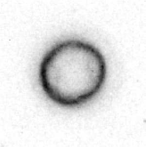
Figure 42: The nebula H 2-13 (PN G 357.2+02.0). The data are presented as in Fig. 17. The morphology is deceptively simple but the velocity profile, especially in [O iii], is complex and the [O iii] line is (unusually) wider than [N ii]. Note that the profile is extracted from the inner arcsecond and not from the bright rim. This may be a bipolar nebula seen pole-on with polar flows contributing to the line broadening.

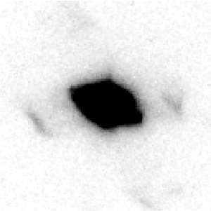
Figure 43: The nebula H 1-46 (PN G 358.5$-$04.2). The data are presented as in Fig. 17. The slit is oriented along the major axis.

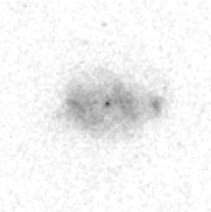
Figure 44: The nebula Al 2-F (PN G 358.5+02.9). The data are presented as in Fig. 17. A quadrupolar nebula.

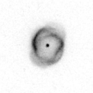
Figure 45: The nebula M 3-40 (PN G 358.7+05.2). The data are presented as in Fig. 17.

Figure 46: The nebula H 1-19 (PN G 358.9+03.4). The data are presented as in Fig. 17. The slit is oriented along the major axis.