Depolarizing Collisions with Hydrogen: Neutral and Singly Ionized Alkaline Earths

Abstract

Depolarizing collisions are elastic or quasielastic collisions that equalize the populations and destroy the coherence between the magnetic sublevels of atomic levels. In astrophysical plasmas, the main depolarizing collider is neutral hydrogen. We consider depolarizing rates on the lowest levels of neutral and singly ionized alkaly-earths Mg i, Sr i, Ba i, Mg ii, Ca ii, and Ba ii, due to collisions with H^∘. We compute ab initio potential curves of the atom-H^∘ system and solve the quantum mechanical dynamics. From the scattering amplitudes we calculate the depolarizing rates for Maxwellian distributions of colliders at temperatures $T\leq$10000 K. A comparative analysis of our results and previous calculations in the literature is done. We discuss the effect of these rates on the formation of scattering polarization patterns of resonant lines of alkali-earths in the solar atmosphere, and their effect on Hanle effect diagnostics of solar magnetic fields.

1. Introduction

Since the discovery of the linearly polarized component of the Fraunhofer spectrum observed close to the solar limb (Stenflo et al., 1983b, a), much effort has been devoted to understand the physical mechanisms involved in its formation, which is dominated by scattering in the continuum and spectral lines (Stenflo, 1994, 1997; Trujillo Bueno & Landi Degl’Innocenti, 1997; Fluri & Stenflo, 1999; Trujillo Bueno et al., 2002; Landi Degl’Innocenti & Landolfi, 2004). Special attention has received, observationally and theoretically, the influence of weak or tangled magnetic fields on resonance line polarization through the Hanle effect Moruzzi & Strumia (1991), which has opened a new diagnostic window for the magnetism in the solar atmosphere (e.g., Stenflo, 1982, 1991; Leroy, 1989; Bommier et al., 1994; Faurobert-Scholl, 1993; Faurobert-Scholl et al., 1995; Lin et al., 1998; Trujillo Bueno, 2001; Trujillo Bueno & Manso Sainz, 2002; López Ariste & Casini, 2005; Trujillo Bueno et al., 2005). By contrast, elastic depolarizing collisions have received relatively little attention in this context, a neglect motivated by their apparent lack of diagnostic value. However, collisions compete with magnetic fields to depolarize the atomic levels, which must be properly accounted for to calibrate Hanle effect diagnostic techniques; besides, by broadening the atomic energy levels, they modulate the magnetic field strength at which the Hanle effect is sensitive (Lamb, 1970).

Alkaline-earth metals, atomic and singly ionized, show some of the strongest resonant lines in the Fraunhofer spectrum and their resonance polarization patterns have proved remarkable too. Their interpretation has posed important theoretical challenges. Thus, the Ca ii infrared triplet and the Mg i $b$-lines (Stenflo et al., 2000) provided the first clear manifestation of the presence of atomic polarization in metastable levels in the solar chromosphere (Manso Sainz & Trujillo Bueno, 2003; Trujillo Bueno, 2001, consistently with our results here, see Section 4); the polarization pattern around the $H$- and $K$-lines of Ca ii (Stenflo et al., 1980; Stenflo, 1980), and the $h$ and $k$-lines of Mg ii (Henze & Stenflo, 1987), arise from the interference between the upper ${}^{2}P$ levels (Stenflo, 1980; Belluzzi & Trujillo Bueno, 2012). Resonance lines of alkali-earths have proved essential to diagnose unresolved fields in the solar atmosphere. The remarkable scattering polarization signal in the Sr i at 460.7 nm (Stenflo et al., 1980; Faurobert et al., 2001; Bommier & Molodij, 2002), in particular, has been extensively observed with the aim of diagnosing tangled magnetic fields in the solar atmosphere (Stenflo, 1982; Faurobert-Scholl, 1993, 1994; Faurobert-Scholl et al., 1995; Bianda et al., 1999; Trujillo Bueno et al., 2004).

Depolarizing collisions in alkali and alkaline earth atoms with a foreign noble gas have been throughly studied theoretically and experimentally (see Lamb & ter Haar, 1971; Omont, 1977; Baylis, 1978, and references therein). However, in the solar atmosphere the most important depolarizing collider is neutral hydrogen (Lamb, 1970). Rough estimates for the depolarizing rates can be obtained from a dipole-dipole van der Waals approximation for the atom-H^∘ (Lamb & ter Haar, 1971, see also Landi Degl’Innocenti & Landolfi 2004). More recently, Derouich et al. (2003b, a, 2004b, 2004a, 2005); Derouich & Barklem (2007) used ab initio interaction potentials and a semi-classical approach using straight line trajectories at different impact parameters. Kerkeni et al. (2000); Kerkeni (2002); Kerkeni & Bommier (2002); Kerkeni et al. (2003) have calculated depolarizing rates with neutral hydrogen with a fully quantum mechanical approach for the interaction Hamiltonian and dynamics. We follow a similar approach here. We computed ab initio potential curves of the atom-H^∘ system and then solved the dynamics within the scattering matrix formalism. From them, we calculated the depolarizing collision rates for a Maxwellian distribution of colliders.

The most important results of the present work are summarized in Table 1, which gives the depolarizing rates for the lowest-lying energy levels of Mg i, Sr i, Ba i, Mg ii, Ca ii, and Ba ii. Figure 3 shows the relative importance of these depolarizing rates in the solar atmosphere as compared to the radiative (polarizing) rates in the main resonance lines of these atoms and ions (Figure 1).

The next section introduces the general theoretical framework used and Section 3 details the calculations performed for each individual atom and ion considered. The impact on the formation of the scattering polarization patterns in the solar atmosphere is discussed in Section 4.

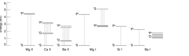
Figure 1.— Partial Grotrian diagrams with the lowest energy levels of the most abundant alkaline earth metals. All levels (except the ${}^{2}S$ and ${}^{2}D$ terms of the Mg i at 8.6 and 8.8 ev) and resonance transitions between them considered in this work are represented. The fine structure energy splitting in Mg and Ca are exaggerated for clarity.

2. Theoretical methodology for Collisional rates

A complete treatment of the Hanle effect on an atom A requires the resolution of the master equations considering radiative transitions, collisional transitions, and the interaction with the magnetic fields. Such formalism has been presented by several authors (e.g., Bommier & Sahal-Brechot, 1978; Bommier, 1980; Landi Degl’Innocenti & Landolfi, 2004). In this work we focus only on deriving the collisional rates caused by collisions with neutral hydrogen atoms, which may have a significant depolarization effect. These collisions are of the type

$$A(\alpha,J,M)+H(S,M_{S})\rightarrow A(\alpha^{\prime},J^{\prime},M^{\prime})+H(S,M^{\prime}_{S}),$$ (1)

between an atom $A$ in a state $\left|\alpha,J,M\right\rangle$ with total angular momentum $J$, magnetic quantum number $M$, and energy $E^{A}_{\alpha,J}$ ($\alpha$ comprises all aditional quantum numbers to characterize the state), and a hydrogen atom $H$ in its ground state, with total angular momentum $S=1/2$, and magnetic quantum number $M_{S}$. We consider only low energy collisions ($E\ll 10$ eV), for which the perturber atom (neutral hydrogen) remains on the ground level after the collision, and the state of the atom under consideration may change only between levels of the same $LS$ term (i.e., $\alpha=\alpha^{\prime}$). We call elastic collisions those for which $J^{\prime}=J$, and quasi-elastic collisions those for which $J^{\prime}\neq J$.

The density matrix of the two atoms system is represented as

$$\left\langle\alpha_{1}J_{1}M_{1};S_{1}M_{S}^{1};{\bf k}_{1}\left|\hat{\rho}\right|\alpha_{2}J_{2}M_{2};S_{2}M_{S}^{2};{\bf k}_{2}\right\rangle,$$

where ${\bf k}=\hbar{\bf v}$ is the wavevector, parallel to the relative velocity vector, ${\bf v}$, between the A and H atoms, of modulus $k=\sqrt{2\mu(E-E^{A}_{\alpha,J}-E^{H}_{S})/\hbar^{2}}$, with $\mu=m_{A}m_{H}/(m_{A}+m_{H})$ being the reduced mass of the colliding atoms and $E$ the total energy of the system. Our interest here focus on the polarization of the atom A, for which we consider its coherence between $J_{1},M_{1}$ and $J_{2},M_{2}$ states. Neutral hydrogen atoms, with density $N_{H^{\circ}}$, interact isotropically with the $A$ atoms, and all the $M_{S}$ sublevels have the weight $1/(2S+1)$. Since we are not interested on the final state of the hydrogen atoms, we sum over all the final states of H^∘ by simply making $S_{1}=S_{2}$ and $M_{S}^{1}=M_{S}^{2}$ (i.e., we consider only diagonal terms in the density matrix). Under these conditions, the reduced density matrix for the $A$ subsystem can be written as

$$\rho_{\alpha J}(M_{1},M_{2})=\sum_{M_{S}}{1\over 2S+1}\int v^{2}dvf(T,v)\int d{\hat{k}}\,\left\langle\alpha JM_{1};\beta SM_{S};{\bf k}\left|\hat{\rho}\right|\alpha JM_{2};\beta SM_{S};{\bf k}\right\rangle,$$ (2)

where $f(T,v)$ is the velocity distribution of the perturbers, here the usual Maxwell-Boltzmann one, ${\hat{k}}\equiv{\hat{v}}$ denotes the polar and azimuthal angles of ${\bf k}$ vector with respect to the frame of the observation. In the above equation the coherence terms between states of A atom with different $\alpha J$ states are neglected. The multipole moments of the density matrix are then defined as

$$\rho^{K}_{Q}(\alpha J)=\sum_{M_{1}M_{2}}(-1)^{J-M}\sqrt{2K+1}\left(\begin{array}[]{ccc}J&J&K\\ M_{1}&-M_{2}&-Q\end{array}\right)\rho_{\alpha J}(M_{1},M_{2}),$$ (5)

where the notation used by Degl’Innocenti (Landi Degl’Innocenti & Landolfi, 2004) has been adopted.

The contribution of collisional transitions to the rate of change of the density matrix elements can be written as (Bommier, 1980; Landi Degl’Innocenti & Landolfi, 2004)

$$\frac{d}{dt}\rho_{\alpha J}(M_{1},M_{2})=\sum_{\alpha^{\prime}J^{\prime}M^{\prime}_{1}M^{\prime}_{2}}C(\alpha JM_{1}M_{2}\leftarrow\alpha^{\prime}J^{\prime}M^{\prime}_{1}M^{\prime}_{2})\quad\rho_{\alpha^{\prime}J^{\prime}}(M^{\prime}_{1},M^{\prime}_{2})$$

$$-{1\over 2}\sum_{\alpha^{\prime}J^{\prime}M^{\prime}M_{3}}\Big{[}C(\alpha^{\prime}J^{\prime}M^{\prime}M^{\prime}\leftarrow\alpha JM_{3}M_{1})\quad\rho_{\alpha J}(M_{3},M_{2})+C(\alpha^{\prime}J^{\prime}M^{\prime}M^{\prime}\leftarrow\alpha JM_{2}M_{3})\quad\rho_{\alpha J}(M_{1},M_{3})\Big{]},$$ (6)

where $C(\alpha^{\prime}J^{\prime}M^{\prime}_{1}M^{\prime}_{2}\leftarrow\alpha JM_{1}M_{2})$ are the corresponding rate constants at a given temperature, defined as

$$C(\alpha^{\prime}J^{\prime}M^{\prime}_{1}M^{\prime}_{2}\leftarrow\alpha JM_{1}M_{2})=N_{H^{\circ}}\int v^{2}dvf(T,v)\,\sigma^{0}(\alpha JM_{1}M_{2};\alpha^{\prime}J^{\prime}M^{\prime}_{1}M^{\prime}_{2}).$$ (7)

In this equation $\sigma^{0}$ is the collisional cross-section averaged over the isotropic distribution of H atoms depending on the collisional energy defined as (Balint-Kurti & Vasyutinskii, 2009; González-Sánchez et al., 2011; Krasilnikov et al., 2013)

$$\sigma^{0}(\alpha JM_{1}M_{2};\alpha^{\prime}J^{\prime}M^{\prime}_{1}M^{\prime}_{2})=\sum_{M_{S},M^{\prime}_{S}}{1\over 2S+1}\int d{\hat{k}}\int d{\hat{k}}^{\prime}\quad[f^{\alpha JM_{1}SM_{S}}_{\alpha^{\prime}J^{\prime}M^{\prime}_{1}S^{\prime}M^{\prime}_{S}}({\hat{k}},{\hat{k}}^{\prime})]^{*}\quad f^{\alpha JM_{2}SM_{S}}_{\alpha^{\prime}J^{\prime}M^{\prime}_{2}S^{\prime}M^{\prime}_{S}}({\hat{k}},{\hat{k}}^{\prime}),$$ (8)

with $f$ being the scattering amplitude, defined below, which relates the amplitude of the products in state $(\alpha^{\prime}J^{\prime}M^{\prime}_{1}S^{\prime}M^{\prime}_{S})$ scattered on a final direction ${\hat{k}}^{\prime}$ from an initial state $(\alpha JM_{1}SM_{S})$ colliding with a relative speed parallel to ${\hat{k}}$.

Equations (2) describing the evolution of the density matrix of an atom under the only action of collisions can be simply added to the equations describing the evolution under radiative processes and external fields (as given, for example, by Bommier, 1980; Bommier & Sahal-Brechot, 1978; Landi Degl’Innocenti & Landolfi, 2004), if the impact approximation is valid. This requires that the collision time be much smaller than the relaxation time due to radiative rates (see Lamb & ter Haar, 1971), which is satisfied in most astrophysical and laboratory plasmas.

The collisional rates can be written as (Omont, 1977; Landi Degl’Innocenti & Landolfi, 2004)

$$C(\alpha^{\prime}J^{\prime}M^{\prime}_{1}M^{\prime}_{2}\leftarrow\alpha JM_{1}M_{2})=(-1)^{J-M_{2}+J^{\prime}-M^{\prime}_{2}}\sqrt{{2J+1\over 2J^{\prime}+1}}\sum_{K}(2K+1)\left(\begin{array}[]{ccc}J^{\prime}&J^{\prime}&K\\ M^{\prime}_{2}&-M^{\prime}_{1}&Q\end{array}\right)\left(\begin{array}[]{ccc}J&J&K\\ M_{2}&-M_{1}&Q\end{array}\right){C}^{(K)}(\alpha^{\prime}J^{\prime}\leftarrow\alpha J)$$ (9)

where ${C}^{K}(\alpha^{\prime}J^{\prime}\leftarrow\alpha J)$ are the multipole components of the collisional rates, which are independent of $Q$ because of the assumed isotropic conditions of the collisional processes (Omont, 1977). Note that the expression of Eq. (9) differs from that given by Omont (1977) in that we have introduced the factor $\sqrt{{2J+1\over 2J^{\prime}+1}}$ to follow the same collisional rate definitions as in Section 7.13 of Landi Degl’Innocenti & Landolfi (2004). The only differences with respect to the notation used by Landi Degl’Innocenti & Landolfi (2004) are that we do not make any notational distinction between downwards and upwards collisional transitions and our use of arrows to indicate the initial and final states. Conversely,

$$C^{(K)}(\alpha^{\prime}J^{\prime}\leftarrow\alpha J)=\sqrt{\frac{2J^{\prime}+1}{2J+1}}\sum_{M_{1}M_{2}M^{\prime}_{1}M^{\prime}_{2}P}(-1)^{J^{\prime}-M^{\prime}_{2}+J-M_{2}}\left(\begin{array}[]{ccc}J^{\prime}&J^{\prime}&K\\ M^{\prime}_{2}&-M^{\prime}_{1}&P\end{array}\right)\left(\begin{array}[]{ccc}J&J&K\\ M_{2}&-M_{1}&P\end{array}\right)C(\alpha^{\prime}J^{\prime}M^{\prime}_{1}M^{\prime}_{2}\leftarrow\alpha JM_{1}M_{2}).$$ (10)

The master equations in terms of the multipole components is given by Eq.(7.101) of Landi Degl’Innocenti & Landolfi (2004), which reads

$$\frac{d}{dt}\rho^{K}_{Q}(\alpha J)=\sum_{J^{\prime}\neq J}\sqrt{\frac{2J^{\prime}+1}{2J+1}}C^{(K)}(\alpha J\leftarrow\alpha^{\prime}J^{\prime})\rho^{K}_{Q}(\alpha^{\prime}J^{\prime})-\left[\sum_{\alpha^{\prime}J^{\prime}\neq\alpha J}C^{(0)}(\alpha^{\prime}J^{\prime}\leftarrow\alpha J)+D^{(K)}(\alpha J)\right]\rho^{K}_{Q}(\alpha J),$$ (11)

where

$$D^{(K)}(\alpha J)=C^{(0)}(\alpha J\leftarrow\alpha J)-C^{(K)}(\alpha J\leftarrow\alpha J)$$ (12)

are the elastic depolarization rates, as defined in equation (7.102) of Landi Degl’Innocenti & Landolfi (2004).

The total depolarizing rate of the $\alpha J$ level is defined as the term within the brackets in Eq. (11):

$$g^{K}(\alpha J)=\bar{C}(\alpha J)+D^{K}(\alpha J),$$ (13)

where

$$\bar{C}(\alpha J)=\sum_{\alpha^{\prime}J^{\prime}}C^{(0)}(\alpha^{\prime}J^{\prime}\leftarrow\alpha J).$$ (14)

are the inelastic rates.

2.1. Scattering amplitudes and cross sections

The scattering wave functions for inelastic collisions for incoming plane waves is subject to the boundary conditions (Curtiss & Adler, 1952)

$$\begin{split}\lim_{R\rightarrow\infty}\Phi_{\alpha JMSM_{S}}({\boldsymbol{k}},{\hat{k}}^{\prime})=&e^{i{\boldsymbol{k}}\cdot{\boldsymbol{R}}}\,|\alpha JM\rangle|SM_{S}\rangle\\ &+i\sum_{\alpha^{\prime}J^{\prime}M^{\prime}S^{\prime}M^{\prime}_{S}}f^{\alpha JMSM_{S}*}_{\alpha^{\prime}J^{\prime}M^{\prime}S^{\prime}M^{\prime}_{S}}({\hat{k}},{\hat{k}}^{\prime}){e^{ik^{\prime}R}\over R\sqrt{k^{\prime}k_{\alpha}}}\,|\alpha^{\prime}J^{\prime}M^{\prime}\rangle|S^{\prime}M^{\prime}_{S}\rangle\end{split}$$ (15)

which determines the scattering amplitude. This $f$ corresponds to a single collision and therefore does not present isotropic symmetry but cylindrical around the incoming velocity ${\hat{k}}$.

The scattering amplitude depends on the three coordinates of ${\bf k}$, involving the resolution of a set of three-dimensional differential equations. To reduce the problem, it is convenient to perform a partial wave expansion, $i.e.$ expand the wave function in terms of eigenfunctions of the total angular momentum, ${\bf J}_{t}={\hbox{\boldmath{$\ell$}\unboldmath}}+{\bf j}$, where $\ell$ is the orbital angular momentum of H with respect to A and ${\bf j}={\bf J}+{\bf S}$ is the angular momentum of the two fragments. Using the partial wave expansion of the incident plane wave, after some algebra (Arthurs & Dalgarno, 1960; Rowe & McCaffery, 1979; Alexander & Davis, 1983; Child, 1996) the scattering amplitude become

$$\begin{split}f^{\alpha JMSM_{S}}_{\alpha^{\prime}J^{\prime}MS^{\prime}M^{\prime}_{S}}({\hat{k}},{\hat{k}}^{\prime})=&\sum_{J_{t}M_{t}}\sum_{jj^{\prime}}\sum_{mm^{\prime}}\sum_{\ell m_{\ell}}\sum_{\ell^{\prime}m^{\prime}_{\ell}}{2\pi\over k}(-1)^{\ell}\,Y^{*}_{\ell m_{\ell}}({\hat{k}})\,Y_{\ell^{\prime}m^{\prime}_{\ell}}({\hat{k}}^{\prime})\,T^{J_{t}}_{n,n^{\prime}}(E)\\ &\times(-1)^{j+j^{\prime}+J+J^{\prime}-\ell-\ell^{\prime}-2S+2M_{t}+m+m^{\prime}}(2J_{t}+1)\sqrt{(2j+1)(2j^{\prime}+1)}\\ &\times\left(\begin{array}[]{ccc}j&\ell&J_{t}\\ m&m_{\ell}&-M_{t}\end{array}\right)\left(\begin{array}[]{ccc}j^{\prime}&\ell^{\prime}&J_{t}\\ m^{\prime}&m^{\prime}_{\ell}&-M_{t}\end{array}\right)\left(\begin{array}[]{ccc}J&S&j\\ M&M_{S}&-m\end{array}\right)\left(\begin{array}[]{ccc}J^{\prime}&S&j^{\prime}\\ M^{\prime}&M^{\prime}_{S}&-m^{\prime}\end{array}\right),\end{split}$$ (16)

where we have introduced the collective quantum number $n\equiv j\ell\alpha JS$ to simplify the notation, and where $M_{t}$ and $m$ are the projections of ${\bf J}_{t}$ and ${\bf j}$ on the z-axis. In this expression $T^{J_{t}}_{n,n^{\prime}}(E)=\delta_{nn^{\prime}}-S^{J_{t}}_{n,n^{\prime}}(E)$, with $S^{J_{t}}_{n,n^{\prime}}(E)$ being the scattering S-matrix, which provides all the information about the collision event for a given total angular momentum $J_{t}$. These S-matrices are obtained by integrating a set of coupled differential equations, as described below.

Following Alexander & Davis (1983), it is convenient to expand the scattering amplitude in terms of spherical tensors, as for the density matrix, whose state-multipoles are given by

$$\begin{split}f^{K^{\prime\prime}}_{Q^{\prime\prime}}(\alpha JSM_{S},{\hat{k}}\rightarrow\alpha^{\prime}J^{\prime}S^{\prime}M^{\prime}_{S},{\hat{k}}^{\prime})=&\sum_{\ell m_{\ell}}\sum_{\ell^{\prime}m^{\prime}_{\ell}}\sum_{KQ}\sum_{K^{\prime}Q^{\prime}}b^{\ell K}_{\ell^{\prime}K^{\prime}}(K^{\prime\prime})Y_{\ell m_{\ell}}({\hat{k}})\,Y_{\ell^{\prime}m^{\prime}_{\ell}}({\hat{k}}^{\prime})\\ &\times(-1)^{\ell+2K^{\prime\prime}+2M_{S}+2M^{\prime}_{S}-Q+2Q^{\prime\prime}}\,(2K+1)(2K^{\prime}+1)\sqrt{2K^{\prime\prime}+1}\\ &\times\left(\begin{array}[]{ccc}K^{\prime}&K&K^{\prime\prime}\\ Q^{\prime}&-Q&-Q^{\prime\prime}\end{array}\right)\left(\begin{array}[]{ccc}S&\ell&K\\ M_{S}&m_{\ell}&Q\end{array}\right)\left(\begin{array}[]{ccc}S^{\prime}&\ell^{\prime}&K^{\prime}\\ M^{\prime}_{S}&m^{\prime}_{\ell}&Q^{\prime}\end{array}\right),\end{split}$$ (17)

with

$$\begin{split}b^{\ell K}_{\ell^{\prime}K^{\prime}}(K^{\prime\prime})=&{2\pi\over k}\sum_{J_{t}jj^{\prime}}T^{J_{t}}_{n,n^{\prime}}(E)(-1)^{J_{t}+J+S}\sqrt{(2j+1)(2j^{\prime}+1)}\\ &\times(2J_{t}+1)\left\{\begin{array}[]{ccc}\ell&J_{t}&j\\ J&S&K\end{array}\right\}\left\{\begin{array}[]{ccc}\ell^{\prime}&J_{t}&j^{\prime}\\ J^{\prime}&S^{\prime}&K^{\prime}\end{array}\right\}\left\{\begin{array}[]{ccc}J^{\prime}&K^{\prime}&J_{t}\\ K&J&K^{\prime\prime}\end{array}\right\}\end{split}$$ (18)

Introducing these last expressions in Eq. (8), and considering no coherent terms, $i.e.$ $M_{1}=M_{2}\equiv M$ and $M^{\prime}_{1}=M^{\prime}_{2}\equiv M^{\prime}$, the inelastic cross section becomes

$$\sigma^{0}(\alpha JM;\alpha^{\prime}J^{\prime}M^{\prime}) = \sum_{K}(-1)^{J+J^{\prime}-M-M^{\prime}}(2K+1)\left(\begin{array}[]{ccc}J&J&K\\ M&-M&0\end{array}\right)\left(\begin{array}[]{ccc}J^{\prime}&J^{\prime}&K\\ M^{\prime}&-M^{\prime}&0\end{array}\right)\quad\sigma^{K}_{\alpha J\rightarrow\alpha^{\prime}J^{\prime}}(E),$$ (23)

where the state multipoles are given by (Kerkeni et al., 2000; Kerkeni, 2002)

$$\sigma^{K}_{\alpha J\rightarrow\alpha^{\prime}J^{\prime}}(E)=\sum_{K^{\prime}}(-1)^{J+J^{\prime}+K+K^{\prime}}(2K^{\prime}+1)\left\{\begin{array}[]{ccc}J^{\prime}&J&K^{\prime}\\ J&J^{\prime}&K\end{array}\right\}\quad B(J,J^{\prime};K^{\prime}).$$ (26)

The rate constant state multipoles of Eq. (10) are directly obtained as

$$C^{(K)}(\alpha^{\prime}J^{\prime}\leftarrow\alpha J)=\sqrt{\frac{2J^{\prime}+1}{2J+1}}N_{H^{\circ}}\int v^{2}dvf(T,v)\,\sigma^{K}_{\alpha J\rightarrow\alpha^{\prime}J^{\prime}}(E).$$ (27)

The $B(J,J^{\prime};K^{\prime})$ quantities are a generalization of the Grawert factors defined as (Kerkeni et al., 2000; Kerkeni, 2002)

$$B(J,J^{\prime};K^{\prime})={1\over 4\pi(2S+1)}\sum_{\ell\ell^{\prime}}\sum_{NN^{\prime}}(2N+1)(2N^{\prime}+1)\quad\left|b^{\ell N}_{\ell^{\prime}N^{\prime}}(K^{\prime})\right|^{2}.$$ (28)

Note that the multipole expansion of the cross section, Eq. (23), presents the same symmetry properties of that of the rates of Eq. (9), associated to the spherical symmetry introduced by the integration over an isotropic distribution of ${\hat{k}}$ in Eq. (8).

2.2. Calculation of S-matrix

Until here, the treatment is general to any atom A, and the full problem has been formalized in terms of the S-matrix elements. In order to evaluate it, we should then particularize to the problem under study, which considers atoms A with no nuclear spin colliding with an Hydrogen atom. The total Hamiltonian of the system is given by

$$H=-{\hbar^{2}\over 2\mu}\left({2\over R}{\partial\over\partial R}+{\partial^{2}\over\partial R^{2}}\right)+{{\hbox{\boldmath{$\ell$}\unboldmath}}^{2}\over 2\mu R^{2}}+H_{el}+H_{SO}^{A},$$ (29)

where $\boldsymbol{\ell}$ is the end-over-end orbital angular momentum associated to the internuclear distance ${\bf R}$.

The total wave function is expanded as

$$\left|\Psi^{J_{t}M_{t}n}_{E}\right\rangle=\sum_{n^{\prime}}{\Phi^{J_{t}M_{t}n}_{n^{\prime}}(R;E)\over R}\,|{\cal Y}^{J_{t}M_{t}}_{n^{\prime}}\rangle.$$ (30)

where ${\cal Y}^{J_{t}M_{t}}_{n}$ are eigenfunctions of the total angular momentum, with eigenvalue $J_{t}$, defined in a space-fixed frame with the z-axis parallel to the observation direction as

$$|{\cal Y}^{J_{t}M_{t}}_{n}\rangle=\sum_{m_{\ell}m}(-1)^{j-\ell+M_{t}}\sqrt{2J_{t}+1}\left(\begin{array}[]{ccc}j&\ell&J_{t}\\ m&m_{\ell}&-M_{t}\end{array}\right)Y_{\ell m_{\ell}}(\theta,\phi)|jm;\alpha JS\rangle,$$ (33)

where $m_{\ell}$, $m$ and $M_{t}$ are the projections of $\boldsymbol{\ell}$, ${\boldsymbol{j}}$ and ${\boldsymbol{J}}_{t}$ on the space-fixed $z$-axis, respectively. In this expression, the wavefunctions of the A(${}^{2S_{A}+1}L_{J}$)+H(${}^{2S+1}S$) fragments are expressed as

$$|jm;\alpha J,S\rangle=\sum_{M,M_{S}}(-1)^{J-S+m}\sqrt{2j+1}\left(\begin{array}[]{ccc}J&S&j\\ M&M_{S}&-m\end{array}\right)|JM;L,S_{A}\rangle|SM_{S}\rangle.$$ (36)

where $|SM_{S}\rangle$ are the eigenfunctions of H, and the A(${}^{2S_{A}+1}L_{J}$) atoms are described by the states

$$|JM;\alpha\equiv L,S_{A}\rangle=\sum_{M_{L},M_{A}}(-1)^{L-S_{A}+M}\sqrt{2J+1}\left(\begin{array}[]{ccc}L&S_{A}&J\\ M_{L}&M_{A}&-M\end{array}\right)|\varphi_{LM_{L}}\rangle|S_{A}M_{A}\rangle$$ (39)

where ${\boldsymbol{J}}={\boldsymbol{L}}+{\boldsymbol{S}}_{A}$ is the total angular momentum of A (${\boldsymbol{L}}$ is the orbital electronic part, described by the functions $|\varphi_{LM_{L}}\rangle$; ${\boldsymbol{S}}_{A}$ the spin of A, described by the $|S_{A}M_{A}\rangle$ functions).

Introducing Equation (30) into the Schrödinger equation, multiplying by $\langle{\cal Y}^{J_{t}M_{t}}_{j\ell;\alpha J}|$, and integrating over electronic and angular variables, the following system of coupled differential equations result:

$$\left\{-{\hbar^{2}\over 2\mu}{\partial^{2}\over\partial R^{2}}+{\hbar^{2}\ell(\ell+1)\over 2\mu R^{2}}+E^{A}_{LS,J}-E\right\}\Phi^{J_{t}M_{t}n}_{n}(R;E)=-\sum_{n^{\prime}}\left\langle{\cal Y}^{J_{t}M_{t}}_{n}\left|{\cal H}_{el}\right|{\cal Y}^{J_{t}M_{t}}_{n^{\prime}}\right\rangle\Phi^{JM\ell n}_{n^{\prime}}(R;E).$$

These close-coupling equations are solved numerically using a Fox-Goodwin-Numerov method (Gadéa et al., 1997), subject to the usual boundary conditions:

$$\Phi^{J_{t}M_{t}n}_{n^{\prime}}(R\rightarrow\infty;E)\propto\sqrt{{\mu\over 2\pi\hbar^{2}}}\left\{\delta_{nn^{\prime}}{e^{-i(kR-\ell\pi/2)}\over\sqrt{k}}-S^{J_{t}}_{nn^{\prime}}(E){e^{i(k^{\prime}R-\ell^{\prime}\pi/2)}\over\sqrt{k^{\prime}}}\right\},$$ (41)

from where the scattering matrix $S^{J_{t}}_{nn^{\prime}}(E)$ is obtained.

The resolution of the close-coupling equations, Eq. (2.2), requires the evaluation of the electronic Hamiltonian matrix elements described below.

2.3. Electronic matrix elements and approximations

The space-fixed functions of Equation (33) are eigenfunctions of $\boldsymbol{\ell}^{2}$ with eigenvalues $\hbar^{2}\ell(\ell+1)$. However, the matrix elements of the electronic terms of the Hamiltonian, $H_{el}$ and $H^{A}_{SO}$, deserve some comments. For treating these two terms we are considering three approximations, which are the commonly used in the previous quantum treatments of collisional depolarization of atoms (Kerkeni et al., 2000; Kerkeni, 2002):

1. First, the spin-orbit is considered as constant as a function of the internuclear distance $R$ and is entirely due to A atom. It is therefore convenient to consider the isolated Hamiltonian of the A atom,

   $$H^{A}=H_{el}^{A}+H_{SO}^{A},$$ (42)

   whose eigenfunctions are those of Equation (39), with eigenvalues $E^{A}_{LS_{A},J}$. Here, we shall use the experimental values obtained from NIST. For this reason, the non-relativistic electronic Hamiltonian is partitioned as

   $$H_{el}=H_{el}^{A}+{\cal H}_{el}.$$ (43)

2. Second, we limit the states of A to a particular $\alpha\equiv LS_{A}$ subspace, thus not allowing transitions between different $L$ values. Thus, $H_{el}^{A}$ is equal in each $\alpha$ subspace. We denote the eigenvalues of $H_{el}$ and ${\cal H}_{el}$ as $V^{S_{t}}_{L\Lambda}(R)$ and ${\cal V}^{S_{t}}_{L\Lambda}(R)$, respectively, with ${\cal V}_{L\Lambda}^{S_{t}}(R)=V_{L\Lambda}^{S_{t}}(R)-E_{L\Lambda}^{S_{t}}$, obtained for each internuclear distance $R$ and with $E_{L\Lambda}^{S_{t}}=V_{L\Lambda}^{S_{t}}(R\rightarrow\infty)$.

3. Finally, the third is the usual Born-Oppenheimer approximation solving the non-relativistic electronic equation

   $$H_{el}|\varphi_{L\Lambda}^{S_{t}}\rangle|S_{t}\Sigma;S_{A}S\rangle=V_{L\Lambda}^{S_{t}}(R)|\varphi_{L\Lambda}^{S_{t}}\rangle|S_{t}\Sigma;S_{A}S\rangle.$$ (44)

   These calculations are performed in a body-fixed frame, with the z-axis along the internuclear vector ${\bf R}$, related by a rotation to the space-fixed frame used in the whole treatment described above. In this new frame, the projections are denoted by greek letters, $\Lambda$ being the projection of ${\bf L}$ on the body-fixed z-axis, while $M_{L}$ is its projection of the space-fixed z-axis. In addition, in this approximation $L$ is not a good quantum number due to the cylindrical symmetry of the problem, but it will be considered as constant since the orbital angular momentum of hydrogen is zero. Finally, the calculations are done for a total spin ${\boldsymbol{S}}_{t}={\boldsymbol{S}}_{A}+{\boldsymbol{S}}$. These $V_{L\Lambda}^{S_{t}}(R)$ eigenvalues are described to the $\left\langle{\cal Y}^{J_{t}M_{t}}_{n}|{\cal H}_{el}|{\cal Y}^{J_{t}M_{t}}_{n^{\prime}}\right\rangle$ matrix elements of the present treatment as described below.

For doing this transformation we shall define the functions for the total spin in the body-fixed frame as

$$|S_{t}\Sigma_{t};S_{A},S\rangle=\sum_{\Sigma_{A},\sigma}(-1)^{S_{A}-S+\Sigma_{t}}\sqrt{2S_{t}+1}\left(\begin{array}[]{ccc}S_{A}&S&S_{t}\\ \Sigma_{A}&\sigma&-\Sigma_{t}\end{array}\right)|S_{A}\Sigma_{A}\rangle|S\sigma\rangle,$$ (47)

and the functions of the fragments, Eq. (36), in the body-fixed frame as

$$|j\Omega;J,L,S_{A},S\rangle = \sum_{S_{t}\Sigma_{t}\Lambda}(-1)^{-S_{t}-S_{A}-S-j+\Omega}\sqrt{(2j+1)(2J+1)(2S_{t}+1)}$$ (53)

$$\times\left\{\begin{array}[]{ccc}S_{t}&S_{A}&S\\ J&j&L\end{array}\right\}\left(\begin{array}[]{ccc}j&S_{t}&L\\ \Omega&-\Sigma_{t}&-\Lambda\end{array}\right)|\varphi_{L\Lambda}^{S_{t}}\rangle|S_{t}\Sigma_{t};S_{A}S\rangle,$$

where the functions $|\varphi_{L\Lambda}^{S_{t}}\rangle$ are the functions obtained in Eq. (44). Finally, the eigenfunctions of well defined total angular momentum in the body-fixed frame are expressed as

$$|W^{J_{t}M_{t}}_{j\Omega;\alpha}\rangle=\sqrt{2J+1\over 4\pi}D^{J_{t}*}_{M_{t}\Omega}(\phi,\theta,0)|j\Omega;\alpha JS\rangle,$$ (54)

where $\theta,\phi$ are the polar angles of ${\boldsymbol{R}}$; $D^{J*}_{M\Omega}$ are rotation Wigner functions (Zare, 1988) corresponding to the $M$ and $\Omega$ projections on the z-axis of the space-fixed and body-fixed frames, respectively.

Using Equations (53)-(54), the ${\cal H}_{el}$ matrix elements in the body-fixed representation take the form

$$\begin{split}\left\langle W^{J_{t}M_{t}}_{j\Omega;\alpha}\left|{\cal H}_{el}\right|W^{J_{t}M_{t}}_{j^{\prime}\Omega^{\prime};\alpha^{\prime}}\right\rangle=&\delta_{\Omega,\Omega^{\prime}}(-1)^{-S_{A}-S_{A}^{\prime}-2S-j-j^{\prime}+2\Omega}\sqrt{(2J+1)(2J^{\prime}+1)(2j+1)(2j^{\prime}+1)}\\ &\times\sum_{S_{t}}(-1)^{-2S_{t}}(2S_{t}+1)\delta_{S,S^{\prime}}\left\{\begin{array}[]{ccc}S_{t}&S_{A}&S\\ J&j&L\end{array}\right\}\left\{\begin{array}[]{ccc}S_{t}&S^{\prime}_{A}&S^{\prime}\\ J^{\prime}&j^{\prime}&L^{\prime}\end{array}\right\}\\ &\times\sum_{\Lambda}\delta_{L,L^{\prime}}{\cal V}_{L\Lambda}^{S_{t}}(R)\sum_{\Sigma_{t}}\left(\begin{array}[]{ccc}j&S_{t}&L\\ \Omega&-\Sigma_{t}&-\Lambda\end{array}\right)\left(\begin{array}[]{ccc}j^{\prime}&S_{t}&L\\ \Omega^{\prime}&-\Sigma_{t}&-\Lambda\end{array}\right).\end{split}$$ (55)

Using the transformations between the space-fixed and body-fixed funtions,

$$|{\cal Y}^{JM}_{j\ell;\alpha}\rangle=\sum_{\Omega}|W^{JM}_{j\Omega;\alpha}\rangle(-1)^{j-\ell+\Omega}\sqrt{2\ell+1}\left(\begin{array}[]{ccc}j&\ell&J\\ \Omega&0&-\Omega\end{array}\right),$$ (56c)

$$|W^{JM}_{j\Omega;\alpha}\rangle=\sum_{\ell}|{\cal Y}^{JM}_{j\ell;\alpha}\rangle(-1)^{\ell-j-\Omega}\sqrt{2\ell+1}\left(\begin{array}[]{ccc}j&\ell&J\\ \Omega&0&-\Omega\end{array}\right),$$ (56f)

the electronic Hamiltonian in the space-fixed frame takes the form

$$\begin{split}\left\langle{\cal Y}^{JM}_{j\ell;\alpha}\left|{\cal H}_{el}\right|{\cal Y}^{JM}_{j^{\prime}\ell^{\prime};\alpha^{\prime}}\right\rangle=&\sum_{\Omega}(-1)^{j+j^{\prime}-\ell-\ell^{\prime}+2\Omega}\sqrt{(2\ell+1)(2\ell^{\prime}+1)}\\ &\times\left(\begin{array}[]{ccc}j&\ell&J\\ \Omega&0&-\Omega\end{array}\right)\left(\begin{array}[]{ccc}j^{\prime}&\ell^{\prime}&J\\ \Omega&0&-\Omega\end{array}\right)\left\langle W^{JM}_{j\Omega;\alpha}\left|{\cal H}_{el}\right|W^{JM}_{j^{\prime}\Omega^{\prime};\alpha^{\prime}}\right\rangle,\end{split}$$

which is equivalent to those reported by Launay & Roueff (1977a, b) for some particular case.

3. Quantum dynamical results

An important feature of the atoms in the alkaline-earth series is the positionning of the two first excited states, as discussed by Allouche et al. (1992). Whereas for Be i and Mg i, the lowest excited states are ${}^{3}P^{\circ}$ and ${}^{1}P^{\circ}$ corresponding to a $ns^{1}np^{1}$ configuration, for Ca i and Sr i the low-lying $(n-1)d$ orbital yields the lowest excited states ${}^{3}P^{\circ}$ and ${}^{3}D$, corresponding to the $ns^{1}np^{1}$ and $ns^{1}(n-1)d^{1}$ configurations, respectively. In Ba i the two first excited states, ${}^{3}D$ and ${}^{1}D$, correspond to the $6s^{1}5d^{1}$ configuration. The situation for cations, with a single valence electron, is analogous but simpler. The importance of these arguments will be discussed below and emphasizes the need of a careful choice of the electronic basis to get accurate atomic energies for the excited states.

The electronic basis set used for magnesium and strontium are the all-electron, augmented correlation-consistent polarized core-valence basis sets, aug-cc-pVTZ (Woon & Dunning, 2013). For calcium the Def2-QZVP basis set was used, obtained from EMSL database (Weigend & Ahlrichs, 2005). For barium, 10 electron small-core scalar relativistic effective core potentials, together with the corresponding valence basis sets (Lim et al., 2006), ECP46MDF, were employed. For hydrogen we used the augmented, correlation-consistent, polarized basis set, aug-cc-pVTZ, of Dunning & Jr. (1989).

The electronic adiabatic potentials, ${\cal V}^{S}_{L\Lambda}(R)$, were calculated in two steps. First, the molecular orbitals were obtained using a complete active space self consistent field (CASSCF) method, with an active space including $ns,np,(n-1)s,(n-1)p,(n-1)d$ orbitals of the alkaline-earth atom, and the $1s$ of hydrogen. In some cases, additional $s,p,d$ orbitals were introduced to properly account for $A^{+}-H^{-}$ ionic states and get the desired degeneracy in the different atomic asymptotes. Second, with these reference states, a multi-reference configuration interaction (MRCI) method (Werner & Knowles, 1988), was used to include the electronic correlation. All these calculations were performed with the MOLPRO package (MOLPRO is a package of ab initio programs designed by H. J. Werner et al., version 2006). Some potential curves are shown in Fig. 2.

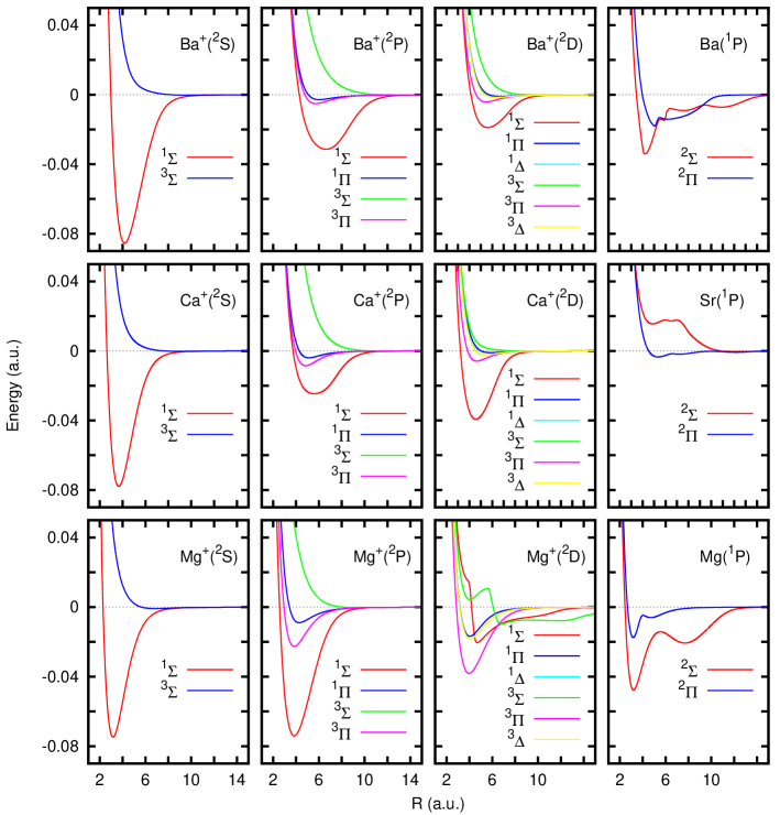
Figure 2.— Calculated ${\cal V}^{S_{t}}_{L\Lambda}(R)$ potential energy curves correlating to the atom A(${}^{2S_{A}+1}L$), as indicated in each panel. In all cases the zero of energy is at the non relativistic energy of atoms at infinite distance.

The close coupled (CC) equations (2.2) were solved for each $LS_{A}$ term, including all possible $J$-levels, $|L-S_{A}|\leq J\leq L+S_{A}$, for all the systems considered in this work. The differential equations were integrated using a spatial grid of 20000 points in the interval $1\leq R\leq 50$ a.u. The ${\cal V}^{S}_{L\Lambda}(R)$ ab initio points, calculated in a considerably coarser grid, were interpolated using cubic splines. The CC equations were integrated for 1000 energies in the interval $E$=10 to 50000 cm^-1, and for each total angular momentum $J^{t}$, $0\leq J^{t}\leq J_{\rm max}$, where $J_{max}$ was determined as that for which the S-matrix becomes diagonal at $E$=50000 cm^-1. Depending on the system and state considered, $J_{\rm max}$ was between 500 and 1500. The S-matrices were then used to calculate $\sigma^{K}_{\alpha J\rightarrow\alpha^{\prime}J^{\prime}}(E)$ according to equation (26). Finally, the state-multipoles of the rates, given in Eq. (9), were calculated by integrating numerically over a Maxwell-Boltzman distribution, Eq. (7), using the energy grid described above. From them the total inelastic rates, Eq. (14), and the depolarization rates, Eq. (13), were obtained.

The rates $\bar{C}(\alpha J)$ (see Eq. 14) and $g^{K}(\alpha J)$ (see Eq. 13) were fitted using the following simple analytical functions ($T$ being the temperature and $N_{H}$ the neutral hydrogen number density):

$$\bar{C}(\alpha J)=a_{0}\times 10^{-9}\left(\frac{T}{5000}\right)^{b_{0}}N_{H},\quad g^{K}=a_{K}\times 10^{-9}\left(\frac{T}{5000}\right)^{b_{K}}N_{H},$$

where $N_{H}$ is the neutral hydrogen number density (in cm^-3), and the $a_{K}$ (s^-1cm³) and $b_{K}$ coefficients are given in Table 1. All the $C^{(K)}(\alpha J\leftarrow\alpha^{\prime}J^{\prime})$ needed to solve Eq.(11) are listed in the appendix. All the inelastic transitions correspond to the same $\alpha=L,S_{A}$ manifold, and therefore do only exist when both $L$ and $S_{A}$ are different from zero and several $J$ states appear. When there are only two $J$ values, these rates fulfill the Einstein-Milne relation (Landi Degl’Innocenti & Landolfi, 2004).

The cations present the simplest structure, with a closed shell core and a single active electron. The $a_{1}$ coefficient for the ground ${}^{2}S$ state increases with the size of the core, from Mg ii to Ca ii, to Ba ii. This is because the larger the cation, the larger the number of partial waves required for convergence, which yields larger cross sections, and inelastic and depolarizing rates. A similar trend is observed for $a_{1}$ in the excited ${}^{2}P^{\circ}$ states of the cations, even when the ${}^{1}\Sigma$ state correlating to Mg ii (3p, ${}^{2}P$) is about twice deeper than in Ca ii and Ba ii (Fig. 2). The $a_{0}$ is significantly smaller for Ba ii (${}^{2}P$) than for Ca ii (${}^{2}P$), while the potential curves involved for these two systems are rather similar (Fig. 2). The reason for this is the strong dependence ($\sim Z^{4}$) of the fine structure splitting with the atomic number $Z$ —the energy separation between the $J=1/2$ and $3/2$ levels is 91.6, 222.9, and 1690.8 cm^-1, for Mg ii, Ca ii and Ba ii, respectively.

The behaviour of the ${}^{2}D$ states of the cations is strikingly different, $a_{0}$ and $a_{1}$ being $\sim$6 times larger for Mg ii than for Ca ii or Ba ii. The reason is that, while in Mg ii the ${}^{2}D$ states correspond to the fourth electronic term, in Ca ii and Ba ii they belong to the second term. This makes the ${}^{1}\Sigma$ and ${}^{3}\Sigma$ potential curves correlating to the Mg ii (${}^{2}D$) cross with the ionic states of Mg i + H⁺. The adiabatic potential energy curves used in the present Born-Oppenheimer quantum ab initio approximation are more involved as a consequence of the avoided crossings (Khemiri et al., 2013). This behaviour is the responsible of the anomaly of the Mg ii (${}^{2}D$) levels.

The neutral alkaline-earth atoms are more complex, since they have a closed shell core surrounded by two electrons, and there are many other ionic states correlating to the different electronic terms of the cations which may cross with the excited electronic states. The ground state is always an isotropic ${}^{1}S$ state, and the main transition is towards the ${}^{1}P^{\circ}$ state. For heavier atoms, the ${}^{1}P^{\circ}$ state produces a progressively more complex structure, due to avoided crossings with ionic and low-lying covalent states. For Mg i (${}^{1}P^{\circ}$) this crossing produce a double well in the ${}^{2}\Sigma$ and ${}^{2}\Pi$ states with a rather long interaction length (Fig. 2). The $a_{i}$ values obtained in this work are very close to those reported by Kerkeni (2002), within 1-2 $\%$, showing that the potential curves are rather similar.

The potential energy curves correlating to Sr i (${}^{1}P^{\circ}$) are very close to those correlating to ${}^{1}D$ state. A precise description of this situation is difficult and the results of the calculations become rather sensitive to the electronic basis used and the method applied. This may be the reason why the present results differ from those of Kerkeni et al. (2003) in about 10-15$\%$. For Ba i the situation is even worse because its adiabatic curves are the result of many avoided crossings between different covalent and ionic states (Allouche et al., 1992), and the ${}^{2}\Sigma$ and ${}^{2}\Pi$ potential energy curves present a very complex structure (Fig. 2). Due to the long range of the interaction, the number of partial waves required to get convergence increases noticeably, producing a significant increase of the inelastic and depolarizing rates, which are far larger than in the other cases studied here.

In the quantum ab initio approach used here and most previous studies (Kerkeni, 2002; Kerkeni et al., 2003), an adiabatic description of the electronic states is used. In this description, the states correlating to given states of the $A(\alpha,J)+H$ fragments change adiabatically as they cross with others, essentially of ionic character. This change is consistent with the commonly used Born-Oppenheimer approximation, in which it is assumed that the electrons move much faster than the nuclei, which allows an instantaneous transition from a covalent $A(\alpha,J)+H$ state to ionic $A^{+}(\alpha^{\prime},J^{\prime})+H^{-}$ or $A^{-}(\alpha^{\prime\prime},J^{\prime\prime})+H^{+}$ states, at the precise distance where their energies coincide.

The opposite (diabatic) situation is the one in which this covalent/ionic transitions are neglected, considering that the $A(\alpha,J)+H$ character is preserved for all the internuclear distances. Such description is the one used in the semiclassical approach of Brueckner (1971); Anstee & O’Mara (1995); Derouich et al. (2003b). This different treatment of the interaction potential may explain the dissagrement found for the depolarization rates obtained for Sr I 460.7 nm line between the adiabatic quantum ab initio method in Table 1 and the diabatic semiclassical method of Faurobert-Scholl et al. (1995). For example, our results for Mg ii(${}^{2}P$) are very close to the ones by Kerkeni (2002) (also adiabatic), but the semiclassical results of Derouich et al. (2003b) are larger by about a $10\%$.

The adiabatic description is better suited for low collision energies while the diabatic one is better at high energies. Actually, a combined description is needed, in which transitions between covalent and ionic states are allowed by including the non-adiabatic couplings, thus allowing transitions among different $L,S_{A}$ manifolds. In order to accomplish this, it is convenient to change from the adiabatic representation, where the couplings show very sharp variations at the crossings, to a diabatic representation that includes the couplings among the different states. Such diabatization procedure has been already done for some of the states of MgH (Belayev et al., 2012) and CaH⁺ (Habli et al., 2011). Some work in this direction is now being done in order to assess the necessity of a more exact treatment for the collisional depolarization of atoms in excited electronic states including inelastic transitions between different $L,S_{A}$ manifolds.

Table 1 $\bar{C}(\alpha J)=a_{0}10^{-9}(\frac{T}{5000})^{b_{0}}N_{H}$ and $g^{K}=a_{K}10^{-9}(\frac{T}{5000})^{b_{K}}N_{H}$ with $K>0$.^e

term	$J$	E(cm-1)a	$a_{0}$	$b_{0}$	$a_{1}$	$b_{1}$	$a_{2}$	$b_{2}$	$a_{3}$	$b_{3}$	$a_{4}$	$b_{4}$	$a_{5}$	$b_{5}$
Mg II(${}^{2}S$, ${}^{2}P$,${}^{2}D$)+H
$3s{,}^{2}S$	1/2	0.0	–	–	2.9704	0.36
$3p{,}^{2}P^{\circ}$	1/2	35669.3	4.1553	0.391	5.8448	0.364
	3/2	35760.9	2.1505	0.354	5.2791	0.344	6.1487	0.360	5.8910	0.366
$4s{,}^{2}S$	1/2	69804.9	–	–	7.2124	0.34
$3d{,}^{2}D$	5/2	71490.2	13.4215	0.345	26.1186	0.349	31.7442	0.3523	33.6754	0.359	35.9476	0.360	33.8079	0.350
	3/2	71491.1	20.1389	0.345	30.3626	0.354	34.7140	0.360	33.9266	0.358
Ca II(${}^{2}S$, ${}^{2}P$,${}^{2}D$)+H
$4s{,}^{2}S$	1/2	0.0	–	–	3.6272	0.40
			–	–	3.2935b	0.451b
$3d{,}^{2}D$	3/2	13650.2	2.3294	0.333	3.9194	0.314	4.3988	0.310	4.1986	0.3124
					3.3700b	0.381b	3.8120b	0.376b	3.6154b	0.380b
	5/2	13710.9	1.5892	0.307	3.4631	0.317	4.0100	0.299	4.4144	0.3015	4.5694	0.307	4.1522	0.314
					2.9078b	0.385b	3.2387b	0.34b1	3.6143b	0.359b	3.7318b	0.353b	3.5506b	0.387b
$4p{,}^{2}P^{\circ}$	1/2	25191.5	4.3445	0.5344	6.8611	0.401
					6.2873b	0.476b
	3/2	25414.4	2.3594	0.450	6.5318	0.350	7.6949	0.378	7.2009	0.395
					6.0059b	0.406b	7.0291b	0.428b	6.6772b	0.418b
Ba II(${}^{2}S$, ${}^{2}P$,${}^{2}D$)+H d
$6s{,}^{2}S$	1/2	0.0	–	–	4.5783	0.39
$5d{,}^{2}D$	3/2	4873.9	1.3053	0.941	4.3374	0.376	5.1832	0.360	5.3721	0.3376
	5/2	5674.8	1.1497	0.6943	4.3606	0.343	4.9580	0.340	5.6322	0.336	5.9298	0.323	5.1728	0.345
$6p{,}^{2}P^{\circ}$	1/2	20261.6	0.5658	1.264	9.6737	0.386
	3/2	21952.4	0.5153	0.708	8.4584	0.379	10.2608	0.413	9.6008	0.399
Mg I(${}^{1}P$, ${}^{3}S$, ${}^{3}P$)+H
$3s3p{,}^{3}P^{\circ}$	0	21850.4	6.4795	0.413
	1	21870.5	4.8804	0.411	6.7143	0.411	7.0615	0.408
	2	21911.2	3.2480	0.402	4.9124	0.395	6.7226	0.401	7.1756	0.409	7.2994	0.413
$3s3p{,}^{1}P^{\circ}$	1	35051.3	–	–	13.696	0.415	11.944	0.437
					13.836c	0.329c	10.79c	0.367c
$3s4s{,}^{3}S$	1	41197.4	–	–	6.1710	0.426	18.5106	0.426
Sr I(${}^{1}P$)+H
$5s5p{,}^{1}P^{\circ}$	1	21698.5	–	–	10.5432	0.30	8.42791	0.38
					8.9875c	0.376c	8.0015c	0.386c
Ba I(${}^{1}P$,${}^{1}D$, ${}^{3}P$, ${}^{3}D$)+H d
$6s5d{,}^{3}D$	1	9034.0	5.6561	0.5814	8.6534	0.3938	10.6750	0.3577
	2	9215.5	5.6386	0.5683	8.7799	0.4296	9.1290	0.4222	9.6180	0.4161	10.4261	0.4008
	3	9596.5	3.4702	0.5797	5.3034	0.4543	6.6440	0.4378	7.6926	0.4198	8.7713	0.4045	9.8750	0.3655
$6s5d{,}^{1}D$	2	11395.4	–	–	9.5977	0.4558	10.0612	0.4483	11.2425	0.4346	9.9601	0.4486
$6s6p{,}^{3}P^{\circ}$	0	12266.0	0.2595	0.8466
	1	12636.6	3.4062	0.8594	9.6736	0.3252	12.1638	0.3022
	2	13514.7	1.3572	0.9596	7.6312	0.3774	11.4646	0.3842	12.5007	0.3975	13.3332	0.4126
$6s6p{,}^{1}P^{\circ}$	1	18060.3	–	–	18.5210	0.4240	16.3480	0.424

^a From the NIST Atomic Spectra Database http://physics.nist.gov/asd (Kramida et al., 2013)

^b From Kerkeni et al. (2003)

^c From Kerkeni (2002)

^d For Ba the isotopes 136 and 138 with zero nuclear spin have been considered, and they give undistinguisable results.

^e The $a_{K}$ coefficients are given in s^-1cm³

4. Depolarizing collisions in the solar atmosphere

Now, we study the effect of the calculated depolarizing elastic collisions on the formation of resonance polarization patterns in the solar atmosphere. In particular, we consider the resonant lines of Mg i, and Mg ii, Sr i, Ca ii, Ba i, and Ba ii listed in Table 2, and a semiempirical model of the quiet solar atmosphere such as the C model of Fontenla et al. (Fontenla et al., 1993, FAL-C).

The generation of atomic polarization in atomic levels is detemined by the radiative rates involving those levels. The radiation field in the solar atmosphere is quasi-thermal and relatively weak, the number of photons per mode being $\bar{n}\ll 1$. For excited levels, radiative rates are therefore, dominated by spontaneous decay (no absorptions to upper lying levels); in ground and metastable levels, the only possible radiative rates are absorptions towards upper lying ones. The mean-life time of an excited level $u$ is thus $\tau_{\rm life}=1/\sum_{\ell}A_{u\ell}$, where $A_{u\ell}$ is the Einstein coefficient for spontaneous emission in the $u\rightarrow\ell$ transition and the sum extends over all $\ell$ levels radiatively connected to $u$; the mean-life time of the ground or metastable level $\ell$ is $\tau_{\rm life}=1/\sum_{u}B_{\ell u}J(\nu_{u\ell})$, where $B_{\ell u}$ is the Einstein coefficient for absorption, $J=\int\phi_{\nu}d\nu\int\frac{d\Omega}{4\pi}I$ is the mean intensity (over the solid angle $\Omega$), integrated over the absorption profile $\phi_{\nu}$, and the sum extends over all the levels radiativelly connected to $\ell$. Thus, consider the singly ionized akaline earths (see Figure 1). For the excited levels ${}^{2}P^{\circ}_{3/2}$, $\tau_{\rm life}^{-1}\approx A_{k}$ in Mg ii, $\tau_{\rm life}^{-1}\approx A_{K}+A_{849.8}+A_{854.2}$ in Ca ii, and $\tau_{\rm life}^{-1}\approx A_{455.4}+A_{585.3}+A_{614.1}$ in Ba ii. For the metastable levels, $\tau_{\rm life}^{-1}({}^{2}D_{3/2})=B_{866.2}J(866.2)+B_{849.8}J(849.8)$, $\tau_{\rm life}^{-1}({}^{2}D_{5/2})=B_{854.2}J(854.2)$, in Ca ii; $\tau_{\rm life}^{-1}({}^{2}D_{3/2})=B_{649.6}J(649.6)+B_{585.3}J(585.3)$, $\tau_{\rm life}^{-1}({}^{2}D_{5/2})=B_{614.1}J(614.1)$, in Ba ii. Analogously, regarding the neutral alkaline earths (see Figure 1), for Mg i, $\tau_{\rm life}^{-1}({}^{3}S)=A_{b_{1}}+A_{b_{2}}+A_{b_{3}}$, $\tau_{\rm life}^{-1}({}^{3}P^{\circ}_{1})=B_{b_{2}}J(b_{2})$, $\tau_{\rm life}^{-1}({}^{3}P^{\circ}_{2})=B_{b_{4}}J(b_{4})$, and $\tau_{\rm life}^{-1}({}^{1}P^{\circ})=A_{285.2}$; for Sr i, $\tau_{\rm life}^{-1}({}^{1}P^{\circ})=A_{460.7}$; for Ba i, $\tau_{\rm life}^{-1}({}^{1}P^{\circ})=A_{460.7}$.

The coefficients $A_{u\ell}$ compiled from the NIST database are tabulated in Table 2, from which the $B_{\ell u}=A_{u\ell}\frac{c^{2}}{2h\nu^{3}}g_{u}/g_{\ell}$ derive ($c$ is the speed of light, $h$ the Planck constant, $\nu$ the frequency of the transition, and $g_{i}=2J_{i}+1$ the degeneracy of the level). The mean intensity $J$ varies at each point in the atmosphere. Deep in the atmosphere the radiation field is trapped and close to Planckian $J\approx B_{\nu}$ ($B_{\nu}$ is the Planck function); in the upper layers of the atmosphere the radiation field may escape through the free boundary and $J$ strongly separates from $B_{\nu}$. The calculation of the actual values of $J$ requires computing the radiation field consistent with the excitation state of the atoms in the atmosphere (non-LTE problem). The population of an atomic level $i$ may be expressed as

$$N_{i}={\cal N}\;10^{A-12}\;\alpha\frac{g_{i}}{u(T)}\exp\left(-\frac{E_{i}}{k_{\rm B}T}\right)b_{i},$$ (57)

where ${\cal N}$ is the total number density of atoms, $A$ is the abundance of the element in the usual logarithmic scale in which $A_{H}=12$ ($A_{\rm Ca}=6.36$, $A_{\rm Mg}=7.58$, $A_{\rm Sr}=2.97$, $A_{\rm Ba}=2.13$; Grevesse et al., 1996), $\alpha$ is the fraction of the ionization state considered (for simplicity, here we assumed it is given according to the Saha formula; Mihalas, 1978), $E_{i}$ the excitation energy of the level, $k_{\rm B}$ the Boltzmann constant, and $T$ the temperature, $g_{i}=2J_{i}+1$ the degeneracy of the level, $u(T)$ the partition function of the ion (we used the tables of Irwin, 1981), and $b_{i}$ the departure coefficient from a purely LTE population. The rigorous calculation of $J$ for the radiation field and the $b_{i}$ for the atomic levels requires the solution of a set of non-linear, non-local, integro-differential equations —the NLTE problem (e.g., Mihalas, 1978). We made the simple, rough estimate $b_{i}\approx 1$ for all the levels of interest, from which the intensity may be obtained integrating the radiative transfer equation

$$\frac{dI}{ds}=-\kappa I+\epsilon,$$ (58)

where

$$\kappa=\frac{h\nu}{4\pi}B_{\ell u}N_{\ell}\phi_{\nu},\quad{\rm and}\quad\epsilon=\frac{h\nu}{4\pi}A_{u\ell}N_{u}\phi_{\nu},$$

are the absorption and emission coefficients, respectively, with $N_{\ell}$ and $N_{u}$ being the population of the lower and upper level of the transition and $\phi_{\nu}$ the Voigt absorption profile. Considering the solar atmosphere as a plane-parallel atmosphere, the element of path along a ray is $ds=dz/\cos\theta$, with $z$ the height and $\theta$ the inclination angle of the ray with respect to the vertical. Equation (58) was numerically integrated using a short-characteristics scheme (Kunasz & Auer, 1988); a Gaussian $N_{\mu}$-point quadrature was used for the angular integration and a trapezoidal $N_{\nu}$-point rule for the frequency integral (here, $N_{\mu}=21$ and $N_{\nu}=11$ were used).

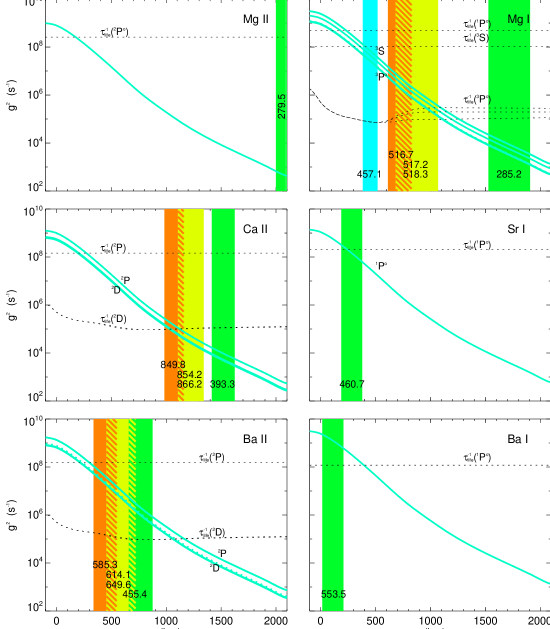
Figure 3.— Variation with height, in a semiempirical solar model atmosphere (FAL-C), of the elastic depolarizing collisional rates $g^{K}$ (solid lines) and radiative relaxation rates (dotted lines) in the lowest levels and resonant transitions of Mg ii, Mg i, Ca ii, Sr i, Ba ii, and Ba i. The curves for $g^{2}$ and $g^{4}$ of the ${}^{2}D$ metastable levels of Ca ii and Ba ii, and the ${}^{3}P$ levels of Mg i, are indistiguishable. Colored bands show the estimated height of formation of the core of the resonant lines indicated (labels in nm), from disk center (left edge) to $\mu=0.1$ (right edge).

Table 2 Atomic data for lines of astrophysical interest^a

$\lambda$ (nm)	lower term	$J_{\ell}$	upper term	$J_{u}$	$A_{u\ell}$ (s-1)
Mg II
279.553 ($k$)	$3s\;{}^{2}S$	1/2	$3p\;{}^{2}P^{\circ}$	3/2	$2.6\times 10^{8}$
280.270 ($h$)		1/2		1/2	$2.6\times 10^{8}$
Ca II
393.366 ($K$)	$4s\;{}^{2}S$	1/2	$4p\;{}^{2}P^{\circ}$	3/2	$1.35\times 10^{8}$
396.847 ($H$)		1/2		1/2	$1.32\times 10^{8}$
849.802	$3d\;{}^{2}D$	3/2	$4p\;{}^{2}P^{\circ}$	3/2	$1.11\times 10^{6}$
854.209		5/2		3/2	$9.9\times 10^{6}$
866.214		3/2		1/2	$1.06\times 10^{7}$
Ba II
455.403	$6s\;{}^{2}S$	1/2	$6p\;{}^{2}P^{\circ}$	3/2	$1.11\times 10^{8}$
493.407		1/2		1/2	$9.53\times 10^{7}$
585.367	$5d\;{}^{2}D$	3/2	$6p\;{}^{2}P^{\circ}$	3/2	$6\times 10^{6}$
614.171		5/2		3/2	$4.12\times 10^{7}$
649.690		3/2		1/2	$3.10\times 10^{7}$
Mg I
285.212	$3s^{2}\;{}^{1}S$	0	$3s3p\;{}^{1}P^{\circ}$	1	$5\times 10^{8}$
457.109	$3s^{2}\;{}^{1}S$	0	$3s4s\;{}^{3}S$	1	$2.54\times 10^{2}$
516.732 ($b_{1}$)	$3s3p\;{}^{3}P^{\circ}$	0	$3s4s\;{}^{3}S$	1	$1.16\times 10^{7}$
517.268 ($b_{2}$)		1		1	$3.46\times 10^{7}$
518.360 ($b_{4}$)		2		1	$5.75\times 10^{7}$
Sr I
460.733	$5s^{2}\;{}^{1}S$	0	$5s5p\;{}^{1}P^{\circ}$	1	$2.01\times 10^{8}$
Ba I
553.548	$6s^{2}\;{}^{1}S$	0	$6s6p\;{}^{1}P^{\circ}$	1	$1.19\times 10^{8}$

^aFrom the NIST Atomic Spectra Database http://physics.nist.gov/asd (Kramida et al. 2013)

For resonance transitions at optical frequencies ($\nu$) and for the temperatures characteristic of the solar atmosphere ($T\sim 6000$ K), $B_{\ell u}J\sim B_{\ell u}B_{\nu}(T)\sim A_{u\ell}\exp(-h\nu/K_{\rm B}T)$ ($K_{\rm B}$ is the Boltzmann constant), i.e., $B_{\ell u}J\ll A_{u\ell}$ and hence, the mean life time of ground and metastable levels ($\ell$) is a few orders of magnitude larger than the radiative life time of excited levels $u$: $\tau_{\rm life}(\ell)\gg\tau_{\rm life}(u)$.

The variation with height of $g^{(K)}$ in the solar atmosphere is dominated by the exponential stratification of density, with just a minor correction from $T$ due to the weak dependence of the collisional rates ($b_{K}\sim 0.3$-0.4 according to Table 1), falling six orders of magnitude from the bottom of the photosphere to the high chromosphere 2000 km above (see Figure 3).

The role of depolarizing collisions on the formation of the scattering polarization patterns is determined by the relative importance of the radiative (polarizing) and the collisional (depolarizing) rates at the height where the line forms. We may estimate the formation height, $H$, of a spectral feature roughly as that for which the optical distance to the free surface (at $z_{\rm max}$) is $\int_{H}^{z_{\rm max}}\kappa dz/\mu\approx 1$. Taking into account the definition of $\kappa$ (after Equation (58)) and Equation (57):

$$\frac{c^{2}}{8\pi^{3/2}\nu^{2}}10^{(A-12)}{\cal N}_{0}\int_{H}^{\infty}\frac{A_{u\ell}}{\Delta\nu_{D}}b_{\ell}\frac{g_{u}\exp(-E_{\ell}/K_{\rm B}T)}{u(T)}\alpha\exp(-z/{\cal H})\frac{dz}{\mu}\approx 1,$$ (59)

where $\Delta\nu_{D}$ is the thermal Doppler width of the transition and a strict exponential stratification ${\cal N}={\cal N}_{0}\exp(-z/{\cal H})$ (${\cal N}_{0}\approx 1.2\times 10^{17}$ cm^-3, ${\cal H}\approx 130$ km for FAL-C), has been assumed for the total number density. Figure 3 shows the regions where the core of several important alkaline-earth resonance lines form (vertical stripes) at different heliocentric distances, from disk center ($\cos\theta=1$; lowest part of the stripe), to $\cos\theta=0.1$ (upper part of the stripe) characteristic of observations close to the solar limb.

The Mg ii $h$ and $k$-lines form very high in the chromosphere, just short of the transition region. At those heights, due to the low density (and despite the temperature rise), the radiative rates of the upper level ${}^{2}P^{\circ}_{3/2}$ is several orders of magnitude larger than the collisional depolarizing rates. The atomic polarization induced in that level will remain largely unaffected by collisions.

Calcium is 16 times less abundant than magnesium and the corresponding Ca ii $H$ and $K$-lines at 396 and 393 nm form $\sim$500 km lower in the chromosphere, but the radiative decay rate of the level ${}^{2}P^{\circ}_{3/2}$ is still orders of magnitude larger than $g^{K}$ and its atomic polarization remains unaffected by depolarizing collisions. The infrared triplet lines between the metastable ${}^{2}D$ levels and the excited ${}^{2}P$ levels form lower in the chromosphere. Interestingly, the $\tau_{\rm life}^{-1}({}^{2}D)$ is larger than $g^{K}$ in that region, which guarantees that the atomic polarization generated in the metastable levels survives to the depolarizing collisions. Certainly this must be the case since it has long been shown that the origin of the observed scattering polarization pattern in this triplet (Stenflo et al., 2000), must be the differential absorption of light polarization components (dichroism) due to the presence of a sizable amount of atomic polarization in the metastable levels (Manso Sainz & Trujillo Bueno, 2003). Yet, $g^{K}$ is still of the order of the radiative rates, which means that the actual values of the observed polarization are modulated by the value of the collisions, and precise values of $g^{K}$ are mandatory for the accurate diagnostic of chromospheric magnetic fields via the Hanle effect in these important lines.

The corresponding $D_{1,2}$ lines of Ba ii (${}^{2}S-{}^{2}P$), and the triplet (${}^{2}D-{}^{2}P$) form even deeper, in the region of the minimum of temperature (see Figure 3). The collisional rates are still unable to compete with the strong radiative rates involving the ${}^{2}P_{3/2}$ level, but they are high enough to completely depolarize the metastable levels ${}^{2}D$.

Mg i is a minority species even in the region of the minimum of temperature which makes it very sensitive to NLTE effects. In fact, our estimate for the ionization fraction $\alpha$ using the Saha-formula grossly overestimates the abundance of Mg iii in the upper part of the chromosphere in NLTE conditions. More realistic calculations show that Mg ii is the dominant ionization state in most of the chromosphere and that, as a consequence, there is a residual but important increase in the column density of Mg i. Correcting for the amount of Mg i in the chromosphere slightly raises the height of formation at disk center of the $b$-lines, but has an important impact for oblique observations close to the limb. The lines then form at $\sim$800-1000 km, a region where the collisional rates are slightly larger than the radiative rates of the metastable lower levels of this triplet $\tau^{-1}_{\rm life}({}^{3}P^{\circ})$, yet not large enough to completely depolarize them. This is important because the Mg i $b$-lines show a clear scattering polarization pattern (Stenflo et al., 2000) whose formation, has been argued, could only be understood by the presence of atomic polarization in the metastable ${}^{3}P^{\circ}$ levels (Trujillo Bueno, 2001).

The Sr i resonant line at 460.7 nm has been extensively used for the diagnostics of unresolved/disorganized/turbulent fields in the solar atmosphere through the Hanle effect (e.g., Stenflo, 1982; Faurobert-Scholl, 1993; Faurobert et al., 2001; Trujillo Bueno et al., 2004; Bommier et al., 2005). One of the reasons for this interest is that it shows one of the largest linear polarization signals in the visible solar limb. The 460.7 nm line forms in the upper photosphere and the close to the limb observations correspond to $\sim 400$ km (Trujillo Bueno et al., 2004). At such height, $g^{K}<\tau_{\rm life}^{-1}$ (Figure 3) and depolarizing collisions cannot destroy the atomic polarization generated in the strong resonance line. Yet, they are of the same order of magnitude and collisions modulate the observed signal. Therefore, accurate depolarizing rates are necessary for precise measurements of the turbulent magnetic fields in the solar photosphere.

5. Conclusions

The main results of this work are summarized in Table 1 and Figure 3. Table 1 gives the effective depolarizing collisional rates averaged over a Maxwellian distribution of velocities for the colliders ($T\leq 10000$ K), for low lying levels of four neutral and singly ionized alkalines of astrophysical relevance. The $C^{(K)}(\alpha J^{\prime}\leftarrow\alpha J)$ collisional rates needed to solve the master equations, Eq.(2), with the radiative terms required for a complete treatment, have been fitted and the corresponding parameters are listed in the appendix.

The cross-sections have been computed from interatomic potentials calculated using the most up-to-date ab initio methods using an adiabatic approach, and the rates using a quantum time-independent close coupling approach. For the excited electronic states there are many curve crossing with ionic states which introduce complicated features in the energy curves considered. At these crossings there are non-adiabatic couplings which may induce inelastic transitions among different $L,S_{A}$ manifolds. Because of the many crossings observed in this work, it is concluded that it is necessary to go beyond the adiabatic quantum ab initio method used here or the diabatic semiclassical method (Brueckner, 1971; Anstee & O’Mara, 1995; Derouich et al., 2003b) in order to incorporate inelastic transitions for these kind of systems, in order to get more realistic results.

Figure 3 summarizes the relative importance of the depolarizing collisions and the (polarizing) radiative rates in the solar atmosphere. We have considered the effect of depolarizing collisions on the polarization pattern of resonance lines of the studied species.

6. Acknowledgments

Financial support by the Spanish Ministry of Economy and Competitiveness through projects CONSOLIDER INGENIO CSD2009-00038 (Molecular Astrophysics: The Herschel and Alma Era), FIS2011-29596-C02 and AYA2010–18029 is gratefully acknowledged. The access to the CESGA computing center, through ICTS grants, is also acknowledged.

7. Appendix

The modeling of the observed spectral line polarization requires the knowledge of all the $C^{(K)}(\alpha^{\prime}J^{\prime}\leftarrow\alpha J)$ collisional rates. In this work we consider the quasi-elastic (or weakly inelastic) rates, with $\alpha^{\prime}=\alpha$. We fitted all such collisional rates by using the following analytical function:

$$C^{(K)}(\alpha J^{\prime}\leftarrow\alpha J)=\sqrt{{2J^{\prime}+1\over 2J+1}}\quad a\times 10^{-9}\left(\frac{T}{5000}\right)^{b}c^{T/5000}N_{H}.$$

The term $c^{T/5000}$ has been added to fit some of the terms presenting very different slopes at low and high temperatures. In general, all the $C^{(K)}(\alpha J\leftarrow\alpha J)$ and $C^{(0)}(\alpha J^{\prime}\leftarrow\alpha J)$ (with $J^{\prime}\neq J$) show a monotonously increasing behavior which is very nicely fitted by the functional form given above. For $K>0$, and $J\neq J^{\prime}$, there are some cases for which the calculated $C^{(K)}(\alpha J^{\prime}\leftarrow\alpha J)$ show an oscillation at low temperatures. Such behavior is not well reproduced without the term $c^{T/5000}$, but in all the cases the fit is good for $T>5000$. The fitting parameters thus obtained for all the systems and electronic terms ($\alpha$) are listed in the following Tables. From these $C^{(K)}(\alpha J^{\prime}\leftarrow\alpha J)$ coefficients the total rate $\bar{C}(\alpha J)$, given in Eq. (14), and the elastic depolarization rates $D^{(K)}(\alpha J)$, given in Eq. (12), are easily obtained. It is worth mentioning that the fits in Table 1 were obtained independently to those listed below. It is also important to note that since the fits to $C^{(K)}(\alpha J^{\prime}\leftarrow\alpha J)$ and $C^{(K)}(\alpha J\leftarrow\alpha J^{\prime})$ were obtained independently, they do not strictly satisfy the detailed balance relationships.

Table 3 Parameters obtained for Mg II

Mg II
term($\alpha$)	$J$	$J^{\prime}$	$K$	$a$	$b$	$c$
$3s,^{2}S$	1/2	1/2	0	22.2697	0.2688	0.8618
	1/2	1/2	1	19.8177	0.2720	0.8197
$3p,^{2}P$	1/2	1/2	0	16.0459	0.1339	1.0269
	1/2	1/2	1	14.9229	0.1484	0.9955
	1/2	3/2	0	3.3010	0.4964	0.9016
	1/2	3/2	1	-0.6678	0.6181	0.7443
	3/2	1/2	0	2.9787	0.3331	1.0189
	3/2	1/2	1	-0.6683	0.5480	0.7675
	3/2	3/2	0	17.6662	0.1534	1.0285
	3/2	3/2	1	14.8318	0.1342	1.0157
	3/2	3/2	2	14.0900	0.1229	1.0080
	3/2	3/2	3	14.4004	0.1279	1.0046
$4s,^{2}S$	1/2	1/2	0	29.4615	0.2790	1.1046
	1/2	1/2	1	22.0850	0.2534	1.1455
$3d,^{2}D$	3/2	3/2	0	36.5529	0.3559	0.9904
	3/2	3/2	1	25.9186	0.3367	1.0004
	3/2	3/2	2	21.4675	0.3197	1.0044
	3/2	3/2	3	22.1888	0.3220	1.0069
	3/2	5/2	0	17.5339	0.4005	0.9449
	3/2	5/2	1	-2.4611	0.3683	0.8772
	3/2	5/2	2	2.6412	0.4185	0.9148
	3/2	5/2	3	-0.5544	0.4104	0.9631
	5/2	3/2	0	17.5517	0.4021	0.9438
	5/2	3/2	1	-2.4640	0.3700	0.8761
	5/2	3/2	2	2.6437	0.4200	0.9138
	5/2	3/2	3	-0.5549	0.4120	0.9620
	5/2	5/2	0	43.7542	0.3627	0.9830
	5/2	5/2	1	30.3133	0.3465	0.9971
	5/2	5/2	2	24.5383	0.3356	1.0018
	5/2	5/2	3	22.6828	0.3278	0.9989
	5/2	5/2	4	20.2225	0.3160	1.0069
	5/2	5/2	5	22.4469	0.3249	1.0059

Table 4 Parameters obtained for Ca II

Ca II
term($\alpha$)	$J$	$J^{\prime}$	$K$	$a$	$b$	$c$
$4s,^{2}S$	1/2	1/2	0	10.1683	0.1461	1.1290
	1/2	1/2	1	6.8879	0.0766	1.1440
$3d,^{2}D$	3/2	3/2	0	11.6422	0.2537	0.9997
	3/2	3/2	1	10.2758	0.2673	0.9805
	3/2	3/2	2	9.8214	0.2698	0.9775
	3/2	3/2	3	9.9750	0.2648	0.9819
	3/2	5/2	0	1.8837	0.3232	1.0090
	3/2	5/2	1	-0.1043	0.2138	0.6809
	3/2	5/2	2	0.1163	0.3383	1.2833
	3/2	5/2	3	-0.0608	0.0704	1.1641
	5/2	3/2	0	1.7165	0.1947	1.1179
	5/2	3/2	1	-0.1054	0.1604	0.6896
	5/2	3/2	2	0.1052	0.1960	1.4333
	5/2	3/2	3	-0.0543	-0.0726	1.3118
	5/2	5/2	0	12.2968	0.2641	0.9974
	5/2	5/2	1	10.5245	0.2613	0.9883
	5/2	5/2	2	9.9563	0.2636	0.9896
	5/2	5/2	3	9.5741	0.2629	0.9872
	5/2	5/2	4	9.4489	0.2622	0.9842
	5/2	5/2	5	9.7655	0.2550	0.9933
$4p,^{2}P$	1/2	1/2	0	10.6365	0.1941	1.0711
	1/2	1/2	1	8.5475	0.2386	1.0475
	1/2	3/2	0	3.8173	0.7415	0.8225
	1/2	3/2	1	-0.8538	1.2265	0.5517
	3/2	1/2	0	3.3951	0.4626	0.9852
	3/2	1/2	1	-0.8643	1.0820	0.5869
	3/2	3/2	0	13.7498	0.3205	1.0098
	3/2	3/2	1	9.5825	0.3292	1.0144
	3/2	3/2	2	8.4721	0.3098	1.0102
	3/2	3/2	3	9.3266	0.3349	0.9747

Table 5 Parameters obtained for Ba II, for the barium isotopes with zero nuclear spin, ¹³⁸Ba and ¹³⁶Ba

Ba II
term($\alpha$)	$J$	$J^{\prime}$	$K$	$a$	$b$	$c$
$6s,^{2}S$	1/2	1/2	0	13.9609	0.1386	1.0841
	1/2	1/2	1	9.9264	0.0790	1.0680
$5d,^{2}D$	3/2	3/2	0	18.4255	0.2735	0.9255
	3/2	3/2	1	15.7971	0.3207	0.8943
	3/2	3/2	2	14.7100	0.3087	0.9012
	3/2	3/2	3	14.3710	0.3080	0.9085
	3/2	5/2	0	1.7446	1.4666	0.6342
	3/2	5/2	1	-0.2700	2.1136	0.4071
	3/2	5/2	2	0.1545	2.3241	0.4218
	3/2	5/2	3	0.0907	3.3058	0.1347
	5/2	3/2	0	1.6072	0.8165	0.8888
	5/2	3/2	1	-0.2804	1.6079	0.5086
	5/2	3/2	2	0.1575	1.7971	0.5363
	5/2	3/2	3	0.1246	3.1623	0.1275
	5/2	5/2	0	17.1487	0.2515	0.9693
	5/2	5/2	1	13.9871	0.2599	0.9609
	5/2	5/2	2	13.4622	0.2621	0.9545
	5/2	5/2	3	12.7033	0.2530	0.9578
	5/2	5/2	4	12.3177	0.2512	0.9629
	5/2	5/2	5	13.2108	0.2582	0.9556
$6p,^{2}P$	1/2	1/2	0	17.8692	0.2161	1.0473
	1/2	1/2	1	8.8049	0.1112	1.0957
	1/2	3/2	0	0.5194	1.5731	0.7797
	1/2	3/2	1	-0.0132	1.9483	0.9342
	3/2	1/2	0	0.4897	0.3255	1.4292
	3/2	1/2	1	-0.0118	0.6236	1.8070
	3/2	3/2	0	19.7847	0.2930	1.0269
	3/2	3/2	1	11.8792	0.2537	1.0423
	3/2	3/2	2	10.3170	0.2242	1.0267
	3/2	3/2	3	10.9570	0.2434	1.0275

Table 6 Parameters obtained for Mg I

Mg I
term($\alpha$)	$J$	$J^{\prime}$	$K$	$a$	$b$	$c$
$3s3p,^{3}P$	0	0	0	5.2652	0.3164	1.0542
	0	1	0	1.4108	0.3435	1.0455
	0	2	0	1.9195	0.5142	0.9203
	1	0	0	1.3689	0.3011	1.0811
	1	1	0	6.7890	0.3075	1.0614
	1	1	1	5.1094	0.3035	1.0548
	1	1	2	4.7392	0.2933	1.0632
	1	2	0	3.2952	0.4699	0.9504
	1	2	1	1.1216	0.5025	0.9375
	1	2	2	-0.4384	0.4947	0.8861
	2	0	0	1.8167	0.4168	0.9868
	2	1	0	3.1625	0.4009	0.9996
	2	1	1	1.0850	0.4405	0.9792
	2	1	2	-0.4205	0.4256	0.9323
	2	2	0	8.5357	0.3056	1.0543
	2	2	1	6.9518	0.2988	1.0563
	2	2	2	5.1478	0.2619	1.0745
	2	2	3	4.7209	0.2446	1.0760
	2	2	4	4.5807	0.2306	1.0815
$3s3p,^{1}P$	1	1	0	21.8188	0.3833	1.0077
	1	1	1	8.1003	0.3276	1.0240
	1	1	2	10.1407	0.3450	0.9925
$3s4s,^{3}S$	1	1	0	39.5285	0.4225	0.9836
	1	1	1	33.0867	0.4151	0.9875
	1	1	2	20.2220	0.3876	1.0022

Table 7 Parameters obtained for Sr I

Sr I
term($\alpha$)	$J$	$J^{\prime}$	$K$	$a$	$b$	$c$
$5s5p,^{1}P$	1	1	0	43.4158	0.4514	0.8079
	1	1	1	34.6220	0.5641	0.7091
	1	1	2	37.0942	0.5247	0.7198

Table 8 Parameters obtained for Ba I, for the barium isotopes with zero nuclear spin, ¹³⁸Ba and ¹³⁶Ba

Ba I
term($\alpha$)	$J$	$J^{\prime}$	$K$	$a$	$b$	$c$
$6s5d,^{3}P$	1	1	0	14.3162	0.2865	1.0169
	1	1	1	11.6651	0.3703	0.9979
	1	1	2	9.6991	0.4113	0.9922
	1	2	0	3.8751	0.7136	0.7996
	1	2	1	1.0372	1.2164	0.7024
	1	2	2	0.6504	0.9258	0.7962
	1	3	0	1.7184	1.2332	0.6865
	1	3	1	-0.4099	1.6277	0.6003
	1	3	2	0.0648	1.5280	0.6417
	2	1	0	3.5544	0.4957	0.9187
	2	1	1	1.0060	1.0547	0.7669
	2	1	2	0.6113	0.7308	0.8949
	2	2	0	12.5009	0.2241	1.0888
	2	2	1	9.2796	0.2221	1.1302
	2	2	2	9.0408	0.2330	1.1230
	2	2	3	8.5488	0.2293	1.1303
	2	2	4	7.7708	0.2212	1.1431
	2	3	0	3.6769	1.0237	0.7401
	2	3	1	1.5593	1.3927	0.6463
	2	3	2	0.8961	1.3228	0.6951
	2	3	3	0.7816	1.3829	0.6559
	2	3	4	0.3919	1.1992	0.7131
	3	1	0	1.6158	0.7694	0.8741
	3	1	1	-0.4331	1.3037	0.6834
	3	1	2	0.0534	0.9093	0.9270
	3	2	0	3.2868	0.6344	0.9303
	3	2	1	1.5085	1.0888	0.7550
	3	2	2	0.8403	0.9830	0.8362
	3	2	3	0.7589	1.0831	0.7636
	3	2	4	0.3883	0.9204	0.8149
	3	3	0	16.3603	0.3644	0.9208
	3	3	1	14.6417	0.3896	0.9057
	3	3	2	13.1621	0.3815	0.9045
	3	3	3	11.8795	0.3712	0.9119
	3	3	4	10.5420	0.3580	0.9228
	3	3	5	9.0805	0.3424	0.9458
	3	3	6	7.3338	0.3232	0.9733
$6s5d,^{1}D$	2	2	0	24.0293	0.4057	0.9585
	2	2	1	15.1879	0.4196	0.8876
	2	2	2	14.4604	0.4057	0.8988
	2	2	3	13.2916	0.4144	0.8892
	2	2	4	14.5496	0.4049	0.9003
$6s6p,^{3}P$	0	0	0	36.4898	0.5360	0.7526
	0	1	0	4.2507	1.0777	0.7470
	0	2	0	0.6928	2.0524	0.5844
	1	0	0	3.9279	0.7297	0.9079
	1	1	0	20.0150	0.2993	0.8131
	1	1	1	12.0838	0.3141	0.8287
	1	1	2	8.4330	0.2368	0.8777
	1	2	0	1.6280	1.7001	0.6576
	1	2	1	0.2266	1.3048	0.8525
	1	2	2	-0.6519	4.0471	0.0337
	2	0	0	0.7328	1.2606	0.8290
	2	1	0	1.6054	1.0751	0.8861
	2	1	1	0.2249	0.6818	1.1432
	2	1	2	-0.5533	3.2715	0.0523
	2	2	0	24.1559	0.4468	0.9130
	2	2	1	17.4109	0.4954	0.9064
	2	2	2	13.2654	0.5063	0.8978
	2	2	3	12.0040	0.4861	0.9038
	2	2	4	11.1925	0.4619	0.8975
$6s6p,^{1}P$	1	1	0	31.4136	0.3874	1.0268
	1	1	1	12.9017	0.3391	1.0644
	1	1	2	15.1697	0.3536	1.0498

References

- Alexander & Davis (1983) Alexander, M. H., & Davis, S. L. 1983, J. Chem. Phys., 79, 227
- Allouche et al. (1992) Allouche, A. R., Nicolas, G., Barthelat, J. C., & Spiegelmann, F. 1992, J. Chem. Phys, 96, 7646
- Anstee & O’Mara (1995) Anstee, S. D., & O’Mara, B. J. 1995, Mon. Not. R. Astron. Soc., 276, 859
- Arthurs & Dalgarno (1960) Arthurs, A. M., & Dalgarno, A. 1960, Royal Society of London Proceedings Series A, 256, 540
- Balint-Kurti & Vasyutinskii (2009) Balint-Kurti, G., & Vasyutinskii, O. 2009, J. Phys. Chem. A., 113, 14281
- Baylis (1978) Baylis, W. E. 1978, in Progress in Atomic Spectroscopy, part A, ed. W. Hanle & H. Kleinpoppen, 1227
- Belayev et al. (2012) Belayev, A. K., Barklem, P., Spielfiedel, A., et al. 2012, Phys. Rev. A, 85, 032704
- Belluzzi & Trujillo Bueno (2012) Belluzzi, L., & Trujillo Bueno, J. 2012, ApJ, 750, L11
- Bianda et al. (1999) Bianda, M., Stenflo, J. O., & Solanki, S. K. 1999, A&A, 350, 1060
- Bommier (1980) Bommier, V. 1980, Astron. Astrophys., 87, 109
- Bommier et al. (2005) Bommier, V., Derouich, M., Landi Degl’Innocenti, E., Molodij, G., & Sahal-Bréchot, S. 2005, A&A, 432, 295
- Bommier et al. (1994) Bommier, V., Landi Degl’Innocenti, E., Leroy, J.-L., & Sahal-Brechot, S. 1994, Sol. Phys., 154, 231
- Bommier & Molodij (2002) Bommier, V., & Molodij, G. 2002, A&A, 381, 241
- Bommier & Sahal-Brechot (1978) Bommier, V., & Sahal-Brechot, S. 1978, Astron. Astrphys., 69, 57
- Brouard et al. (2009) Brouard, M., Bryant, A., Chang, Y.-P., et al. 2009, J. Chem. Phys., 130, 044306
- Brueckner (1971) Brueckner, K. A. 1971, ApJ, 169, 621
- Child (1996) Child, M. S. 1996, Molecular Collision Theory, Dover Publications, Inc.
- Curtiss & Adler (1952) Curtiss, C. F., & Adler, F. T. 1952, J. Chem. Phys., 20, 249
- Dagdigian & Alexander (2009) Dagdigian, P. J., & Alexander, M. H. 2009, J. Chem. Phys., 130, 094303
- Derouich & Barklem (2007) Derouich, M., & Barklem, P. S. 2007, A&A, 462, 1171
- Derouich et al. (2005) Derouich, M., Barklem, P. S., & Sahal-Bréchot, S. 2005, A&A, 441, 395
- Derouich et al. (2003a) Derouich, M., Sahal-Bréchot, S., & Barklem, P. S. 2003a, A&A, 409, 369
- Derouich et al. (2004a) —. 2004a, A&A, 426, 707
- Derouich et al. (2004b) —. 2004b, A&A, 414, 373
- Derouich et al. (2003b) Derouich, M., Sahal-Bréchot, S., Barklem, P. S., & O’Mara, B. J. 2003b, A&A, 404, 763
- Dunning & Jr. (1989) Dunning, T. H., & Jr. 1989, J. Chem. Phys., 90, 1007
- Faurobert et al. (2001) Faurobert, M., Arnaud, J., Vigneau, J., & Frisch, H. 2001, A&A, 378, 627
- Faurobert-Scholl (1993) Faurobert-Scholl, M. 1993, A&A, 268, 765
- Faurobert-Scholl (1994) —. 1994, A&A, 285, 655
- Faurobert-Scholl et al. (1995) Faurobert-Scholl, M., Feautrier, N., Machefert, F., Petrovay, K., & Spielfiedel, A. 1995, A&A, 298, 289
- Fluri & Stenflo (1999) Fluri, D. M., & Stenflo, J. O. 1999, A&A, 341, 902
- Fontenla et al. (1993) Fontenla, J. M., Avrett, E. H., & Loeser, R. 1993, ApJ, 406, 319
- Gadéa et al. (1997) Gadéa, F. X., Berriche, H., Roncero, O., Villarreal, P., & Delgado-Barrio, G. 1997, J. Chem. Phys., 107, 10515
- González-Sánchez et al. (2011) González-Sánchez, L., Vasyutinskii, O., Zanchet, A., Sanz-Sanzc, C., & Roncero, O. 2011, Phys. Chem. Chem. Phys., 13, 13656
- Grevesse et al. (1996) Grevesse, N., Noels, A., & Sauval, A. J. 1996, in Astronomical Society of the Pacific Conference Series, Vol. 99, Cosmic Abundances, ed. S. S. Holt & G. Sonneborn, 117
- Habli et al. (2011) Habli, H., Dardouri, R., Oujia, B., & Gadéa, F. X. 2011, J. Phy. Chem. A, 115, 14045
- Henze & Stenflo (1987) Henze, W., & Stenflo, J. O. 1987, Sol. Phys., 111, 243
- Irwin (1981) Irwin, A. W. 1981, ApJS, 45, 621
- Kerkeni (2002) Kerkeni, B. 2002, A&A, 390, 783
- Kerkeni & Bommier (2002) Kerkeni, B., & Bommier, V. 2002, A&A, 394, 707
- Kerkeni et al. (2000) Kerkeni, B., Spielfiedel, A., & Feautrier, N. 2000, A&A, 358, 373
- Kerkeni et al. (2003) —. 2003, A&A, 402, 5
- Khemiri et al. (2013) Khemiri, N., Dardouri, R., Oujia, B., & Gadéa, F. X. 2013, J. Phys. Chem. A, 117, 8915
- Kramida et al. (2013) Kramida, A., Ralchenko, Y., Reader, J., & NIST ASD Team. 2013, NIST Atomic Spectra Database (version 5.1)Online Available: http://physics.nist.gov/asd
- Krasilnikov et al. (2013) Krasilnikov, M. B., Popov, R. S., Roncero, O., et al. 2013, J. Chem. Phys., 138, 244302
- Kunasz & Auer (1988) Kunasz, P., & Auer, L. H. 1988, J. Quant. Spec. Radiat. Transf., 39, 67
- Lamb (1970) Lamb, F. K. 1970, Sol. Phys., 12, 186
- Lamb & ter Haar (1971) Lamb, F. K., & ter Haar, D. 1971, Phys. Rep., 2, 253
- Landi Degl’Innocenti & Landolfi (2004) Landi Degl’Innocenti, E., & Landolfi, M. 2004, Polarization in spectral lines, Kluwer Academic Publishers, ASTROPHYSICS AND SPACE SCIENCE LIBRARY, Vol. 307
- Launay & Roueff (1977a) Launay, J. M., & Roueff, E. 1977a, A&A, 56, 289
- Launay & Roueff (1977b) Launay, J.-M., & Roueff, E. 1977b, Journal of Physics B Atomic Molecular Physics, 10, 879
- Leroy (1989) Leroy, J. L. 1989, in Astrophysics and Space Science Library, Vol. 150, Dynamics and Structure of Quiescent Solar Prominences, ed. E. R. Priest, 77–113
- Lim et al. (2006) Lim, I. S., Stoll, H., & P. Schwerdtfeger, J. 2006, Chem. Phys., 124, 034107
- Lin et al. (1998) Lin, H., Penn, M. J., & Kuhn, J. R. 1998, ApJ, 493, 978
- López Ariste & Casini (2005) López Ariste, A., & Casini, R. 2005, A&A, 436, 325
- Manso Sainz & Trujillo Bueno (2003) Manso Sainz, R., & Trujillo Bueno, J. 2003, Physical Review Letters, 91, 111102
- Mihalas (1978) Mihalas, D. 1978, Stellar atmospheres 2nd edition, San Francisco, W. H. Freeman and Co., 1978. 650 p.
- MOLPRO is a package of ab initio programs designed by H. J. Werner et al. (version 2006) MOLPRO is a package of ab initio programs designed by H. J. Werner, M., Knowles, P. J., with contributions from, et al. version 2006
- Moruzzi & Strumia (1991) Moruzzi, G., & Strumia, F. 1991, The Hanle Effect and Level-Crossing Spectroscopy, Plenum Press
- Omont (1977) Omont, A. 1977, Progress in Quantum Electronics, 5, 69
- Rowe & McCaffery (1979) Rowe, M. D., & McCaffery, A. J. 1979, in Laser-Induced Processes in Molecules, ed. K. L. Kompa & S. D. Smith, 66
- Stenflo (1980) Stenflo, J. O. 1980, A&A, 84, 68
- Stenflo (1982) —. 1982, Sol. Phys., 80, 209
- Stenflo (1991) —. 1991, in The Hanle Effect and Level-Crossing Spectroscopy, ed. G. Moruzzi & F. Strumia (Plenum Press), 237
- Stenflo (1994) —. 1994, Solar Magnetic Fields, Kluwer Academic Publishers, Dordrecht, ASTROPHYSICS AND SPACE SCIENCE LIBRARY, Vol. 189
- Stenflo (1997) —. 1997, A&A, 324, 344
- Stenflo et al. (1980) Stenflo, J. O., Baur, T. G., & Elmore, D. F. 1980, A&A, 84, 60
- Stenflo et al. (2000) Stenflo, J. O., Keller, C. U., & Gandorfer, A. 2000, A&A, 355, 789
- Stenflo et al. (1983a) Stenflo, J. O., Twerenbold, D., & Harvey, J. W. 1983a, A&AS, 52, 161
- Stenflo et al. (1983b) Stenflo, J. O., Twerenbold, D., Harvey, J. W., & Brault, J. W. 1983b, A&AS, 54, 505
- Trujillo Bueno (2001) Trujillo Bueno, J. 2001, in Astronomical Society of the Pacific Conference Series, Vol. 236, Advanced Solar Polarimetry – Theory, Observation, and Instrumentation, ed. M. Sigwarth, 161
- Trujillo Bueno et al. (2002) Trujillo Bueno, J., Casini, R., Landolfi, M., & Landi Degl’Innocenti, E. 2002, ApJ, 566, L53
- Trujillo Bueno & Landi Degl’Innocenti (1997) Trujillo Bueno, J., & Landi Degl’Innocenti, E. 1997, ApJ, 482, L183
- Trujillo Bueno & Manso Sainz (2002) Trujillo Bueno, J., & Manso Sainz, R. 2002, Nuovo Cimento C Geophysics Space Physics C, 25, 783
- Trujillo Bueno et al. (2005) Trujillo Bueno, J., Merenda, L., Centeno, R., Collados, M., & Landi Degl’Innocenti, E. 2005, ApJ, 619, L191
- Trujillo Bueno et al. (2004) Trujillo Bueno, J., Shchukina, N., & Asensio Ramos, A. 2004, Nature, 430, 326
- Weigend & Ahlrichs (2005) Weigend, F., & Ahlrichs, R. 2005, PCCP, 7, 3297
- Werner & Knowles (1988) Werner, H. J., & Knowles, P. J. 1988, J. Chem. Phys., 89, 5803
- Woon & Dunning (2013) Woon, D. E., & Dunning, J. T. H. 2013, unpublished
- Zare (1988) Zare, R. 1988, Angular Momentum, John Wiley and Sons, Inc.