Use of Correlation Matrix to Assess the Stirring Performance of a Reverberation Chamber: a Comparative Study

Abstract

The use of correlation matrices to evaluate the number of uncorrelated stirrer positions of reverberation chamber has widespread applications in electromagnetic compatibility. We present a comparative study of recent techniques based on multivariate correlation functions aimed at relating space-frequency inhomogeneities/anisotropies to the reduction of uncorrelated positions. Full wave finite-difference time domain simulations of an actual reverberation chamber are performed through an in-house parallel code. The efficiency of this code enables for capturing extensive inhomogeneous/anisotropic spatial volumes (frequency ranges). The concept of threshold crossing is revised under the light of random field sampling, which is important to the performance of arbitrary reverberation chambers.

I Introduction

Performances of a mode-stirred reverberation chamber (RC) in electromagnetic compatibility (EMC) applications are intimately related to the number of independent cavity realizations [1]. Unambiguous evaluation of the number of independent stirrer positions is still under investigation [2]. Current approaches rely on the autocorrelation of fields sampled at single site inside the working volume (WV) of the RC. The coherence time is based on the autocorrelation function [3]. Previous investigators showed that, despite inside the WV, by considering only one chamber site results in a high spatial variability of the autocorrelation coefficient [4, 5, 6]. This experimental evidence is of crucial importance as the commonly accepted notion of independence for a stirrer position is just defined by the $\rho_{e}=e^{-1}$ threshold crossing of the autocorrelation coefficient. Even though it brings about a simple and effective criterion, this perspective is provably incomplete and uncertain in evaluating whether members of the cavity ensemble is strictly “independent” each other. To this regard, the threshold $\rho_{e}$ is typically associated with the concept of “uncorrelation” rather than “independence”. Those inspections lead to consider a correlation matrix having each entry defined by the correlation between two of the total $N_{s}$ stirrer positions. Of course, the dimension of the so defined correlation matrix is given by $N_{s}\times N_{s}$. In a good RC, we expect a low value for many correlation matrix elements, i.e. many stirrer position pairs are “low correlated”.

According to this multivariate approach, an alternative way of evaluating the number of uncorrelated positions of mechanical mode-stirrers is based on the calculation of the correlation matrix through a grid of $N_{w}$ spatial points, selected among an arbitrary volume of the chamber [7]. Another recent application of the correlation matrix involves single-point measurements through a wide frequency and to evaluate “uncorrelated frequencies” rather than spatial points [8]. This way proves more fast and efficient as populating spatial correlation matrix requires for a large amount of field/power measurements. Hybrid techniques can also be conceived based on the correlation matrix. Spatial point and frequency point data can be combined to check stirring performance.

In this work we review existing multivariate strategies grounded on the correlation matrix that are important to assess RC performances. The typical framework we use to test different performance indicators is a reverberation chamber equipped with a “carousel” mode-stirrer [9]. Being based on multispatial multifrequency sampling, these indicators can be used in arbitrary dynamic and complex wave environment. In particular, the mode stirrer can be either present as in RCs or absent as in wave chaotic billiards or enclosures [10, 11]. Observations are useful to explore the physics of electromagnetic reverberation beyond overmoded regime, and to create finite sets of realizations behaving closely to ideal statistical ensembles. There is room to think that judicious multi-resolved field sampling could lead to a lower chamber lowest usable frequency (LUF) [1].

The strategies being used through the rest of the paper are focused on the evaluation of:

1. uncorrelated stirrer positions adopting a spatial correlation matrix (henceforth referred as “US–PM”);

2. uncorrelated stirrer positions adopting a frequency correlation matrix (henceforth referred as “US–FM”);

3. uncorrelated frequency steps adopting a spatial correlation matrix for a single stirrer position (henceforth referred as “UF–PM”).

In any strategy we analyze the effect of varying the involved parameters, number and distance of frequency and spatial points, and we compare results to those obtained applying the 1–D circular autocorrelation method.

Finally, of interest in RC theory, we propose and use strategies for the analysis of:

1. the uncorrelated frequency steps adopting a stirrer position correlation matrix at a single spatial point (henceforth referred as “UF–SM”);

2. uncorrelated spatial points adopting a stirrer position correlation matrix for each single frequency (henceforth referred as “UP–SM”);

3. uncorrelated spatial points adopting a frequency correlation matrix (henceforth referred as “UP–FM”).

\psfrag{x}{\scriptsize{x}}\psfrag{y}{\scriptsize{y}}\psfrag{z}{\scriptsize{z}}\psfrag{Lx}{\scriptsize{$L_{x}$}}\psfrag{Ly}{\scriptsize{$L_{y}$}}\psfrag{Lz}{\scriptsize{$L_{z}$}}\psfrag{Hs}{\scriptsize{$h$}}\psfrag{De}{\scriptsize{$d_{e}$}}\psfrag{Di}{\scriptsize{$d_{i}$}}\includegraphics[width=180.67499pt]{geo_camera_3D.eps}

Figure 1: Geometry of the reverberation chamber (RC) equipped with a “carousel” stirring system. The simulated RC is that of Ancona EMC laboratory, it is $L_{x}=6$ m long, $L_{y}=4$ m wide and $L_{z}=2.5$ m height. The vertical plates are $h=2.4$ m high and they have a Z-folded shape. The rotating system describes a cylindrical volume whose base is centered in $x=4$ m and $y=2$ m, the external diameter is $d_{e}=3.8$ m and the internal diameter is $d_{i}=3.3$ m.

II RC Performance Indicators

The use of the circular autocorrelation function (ACF) is well accepted for evaluating the number of independent stirrer positions [1]. More advanced methods based on the ACF have been proposed to assess the performances of mode-tuned reverberation chambers (MTRC) [12, 4]. Recently, the concept of multi-resolution for the construction of correlation matrices in MTRC is attracting the interest of the scientific community [13]

The definition of independent stirrer positions based on a multivariate field perspective has been pioneered in [2, 7]. In [5], the number of uncorrelated positions are related to the number of independent eigenvalues of the correlation matrix $\ushortdw{R}_{s}$. In particular, $\ushortdw{R}_{s}$ is populated by Pearson correlation coefficients (PCC). Those elements are calculated as two-point correlation functions between two arbitrary points, and therefore require for multi-resolved field sampling. This has been achieved through a “platform stirring” strategy [5]. From information theoretic arguments, it turns out that the number of independent eigenvalues is

$$N_{\rm eff}=\frac{\textrm{Tr}^{2}\left[\ushortdw{R}_{s}\right]}{\textrm{Tr}\left[\ushortdw{R}_{s}^{2}\right]}\,\,.$$ (1)

This perspective has the advantage to be threshold-less, i.e., the elements of $\ushortdw{R}_{s}$ do not need to be tested against the empirical $e^{-1}$ limit to achieve $N_{\rm eff}$. Threshold-based approaches currently adopted in the IEC normative [1] rely on single point circular autocorrelation coefficient (CC) to evaluate $N_{\rm eff}$. With respect to the IEC method, usage of (1) underestimates $N_{\rm eff}$.

A similar philosophy is adopted in [8] where the concern is the number of uncorrelated measurements rather than stirrer positions. The measurement correlation has been defined in terms of the maximum Renyì entropy, again based on the eigenvalue of the correlation matrix. In particular, given the maximum entropy achievable through $N_{s}$ measurements

$$S_{2}=\log\left(N_{\rm eff}\right)\,\,,$$ (2)

it is straightforward to have an estimation of the number of uncorrelated measurements reading

$$N_{\rm eff}=e^{S_{2}}\,\,.$$ (3)

Since $S_{2}$ can be calculated from the eigenvalues of $\ushortdw{R}_{s}$, then

$$N_{\rm eff}=\frac{\left(\sum_{m=1}^{N_{s}}\lambda_{m}\right)^{2}}{\sum_{m=1}^{N_{s}}\lambda_{m}^{2}}\,\,.$$ (4)

The analogies between between (4) and (1) are many, and essentially they constitute the same formula achieved through different perspectives [14]. The advantage of (4) is that the correlation matrix can be populated through a frequency scanning, i.e., a frequency sampling would lead to $\ushortdw{R}_{f}$ as in [8], rather than the spatial scanning, leading to $\ushortdw{R}_{s}$. It is worth remarking that the estimator (1), used in different versions in [8] and [5], is polarized, and the estimated number of uncorrelated positions $N_{\rm eff}$, based on $M$ space/frequency points, is given by

$$\frac{N_{\rm eff}}{N_{s}}=\frac{1}{1+\frac{N_{s}}{M}}\,\,,$$ (5)

which converges to $N_{\rm eff}$ for a relatively high number of degrees of freedom $M$, i.e., $M\gg N_{s}$. Equation (5) can be demonstrated by noting that the correlation matrix can be expanded in true principal components (PC) [14]. Inherently, it has been recently demonstrated that the RC field admits PC decomposition of the stirring process in empirical (time-domain) modes, called as “eigenstirrings” [15]. Therefore, (5) can be also used to perform a systematic correction of the estimates if we make use of (1) to evaluate the number of effective stirrer positions with a few finite difference time domain (FDTD) lattice points [7].

Based on an entropic perspective, we can use (4) to carry out the calculation of uncorrelated stirrer positions through either $\ushortdw{R}_{s}$ or $\ushortdw{R}_{f}$. It has been already acknowledged that the production of entropy from scattering processes over finite regions of space is important to evaluate the degrees of freedom of a complex EM system [16]. A thorough study of the time-domain entropy generation in RC has been performed in [17], through numerical FDTD simulations of an actual RC, and the linear increase of entropy at early times was proven to saturate at the maxentr limit (2) which converges to the high-frequency estimate. This behavior is typical of multi-component (many-body) complex systems and has been observed in quantum many-body systems operating in chaotic regime [18].

A step forward has been carried out in [19] through the evaluation of uncorrelated pairs in the correlation matrix. This method grasps on graph theory to estimate the number of uncorrelated stirrer positions. A graph is developed where each node corresponds to a stirrer position, and an arc is formed when the correlation between two positions $(i,j)$ satisfies the cutoff condition [1]

$$r_{ij}=\left[\ushortdw{R}_{s}\right]_{ij}\leq\e^{-1}\left[1-\frac{7.22}{\left(N_{s}^{2}\right)^{0.64}}\right]\,\,.$$ (6)

Equation (6) is an extension of the correlation threshold $\rho_{e}$ based on sampling theory. The author then uses standard algorithms to search for the so-called “maximum clique” of the graph, and identifies it as the maximum number of uncorrelated positions. The result is a graphical method to count the number of uncorrelated positions through a direct test of uncorrelated node pairs. The method in [2, 4] relies on a threshold, while the methods proposed in [5, 6] do not rely on it, i.e., they can be classified as threshold-less.

The presence of a threshold should not be taken necessarily as a limitation. Actually, its physical significance will become clear in a random sampling perspective, where we imagine to populate $\ushortdw{R}_{s,f}$ with fluctuating elements. Following this philosophy, we decided to introduce a generalized threshold-based procedure to estimate the number of uncorrelated positions, by exploiting information of an extended reverberation (sub) space rather than a single point. The generality of the method resides in the fact that the sampling over multiple spatial points/frequencies has been extended to an arbitrary reverberant subspace independently on the a-priori definition of a working volume, and beyond the orientation of the DUT. The mathematical procedure is detailed in [7]. The number of uncorrelated stirrer positions comes from counting the number of elements in $\ushortdw{R}_{s,f}$ that are below the threshold (6). Each element has the meaning of a correlation between two cavity sub-spaces (calculated through a discrete space/frequency lattice [20] generated from two different stirrer configurations. More precisely, this number is obtained by taking account of the symmetry properties of $\ushortdw{R}_{s,f}$, and of the fact that $r_{ii}=1$, hence

$$N_{\rm eff}=\frac{N_{s}^{2}}{\#\left[\ushortdw{R}_{s,f}>r\ushortdw{1}\right]}\,\,,$$ (7)

where $\#\left[\cdot\right]$ is the counting operator, $\ushortdw{1}$ is the a square matrix of dimension $N_{s}$, where all elements are 1. When two stirrers are used in an RC, we follow the procedure described in [21]. Here, the case involving $\ushortdw{R}_{s}$ corresponds to US–PM, while the case involving $\ushortdw{R}_{f}$ corresponds to US–FM.

Interestingly, besides stirrer positions, our method can be used to evaluate the number of uncorrelated spatial points given measurements from a set of stirrer positions (US–SM, UP–FM). Also, the number of uncorrelated working frequencies can be estimated from stir sequences (UF–SM), or spatial lattice sampling (UF–SM).

III Full-wave simulations and results

We now evaluate the number of uncorrelated stirrer positions of an actual RC. In particular, we focus on the stirring performances of the “carousel” stirrer previously studied in [9]. Figure 1 shows the detailed geometry: the stirrer consists of equispaced metallic $z$-folded blades. Its rotation describes a cylindrical volume which bounds the uniformity volume of the chamber, i.e., the working volume (WV).

According to the method discussed in Section II, we do not restrict our investigations to an a-priori defined working volume, further requiring a calibration protocol such as that describe in [1, A.5].

Full wave FDTD simulations of the RC have been recently used by other investigators [22, 23, 24]. An in-house FDTD code, optimized for BlueGene computer architecture [25, 26], is used to perform a full wave simulation of the Ancona’s RC. The EM fields can then be sampled over a dense grid of spatial points (sampling lattice), for an arbitrary number of stirrer positions [7].

The RC is then discretized in $201\times 134\times 84$ cubic cells with a side of $30$ mm, the FDTD time step is $\Delta t=50$ ps, and the number of iterations necessary to analyze the entire structure is found to be $206\,748$. Frequency data are obtained by fast Fourier transform (FFT). Figure 1 shows the sampling lattice (gold solid line grid) adopted in the simulations, where the $N_{w}$ points are 0.15 m equispaced.

The discrete (total or Cartesian) field $E_{(m_{i},m_{j},m_{k})}^{\left(\tau\right)}$ is picked up at $N_{w}$ spatial points $(m_{i}\Delta x,m_{j}\Delta y,m_{k}\Delta z)$ of the sampling grid, for each stir state $\tau_{i}=i\Delta\theta$, $i=1,\ldots,N_{s}$, with $\Delta\theta$ angular stirrer step, and $N_{s}$ total number of stirrer positions considered in the analysis. In discretizing the continuous stirring, we assumed that the “uncorrelation angle” of the carousel stirrer is greater than $\Delta\theta$. The correlation is then computed by using $N_{p}$ field values. In particular, for the total electric field we have $N_{p}=N_{w}$, while for the three separate Cartesian components we have $N_{p}=3N_{w}$.

The RC is simulated for $512$ (equispaced) stirrer angles, and for each angle the three Cartesian field components are computed in a grid of $8\times 8\times 8=512$. All the above field data were saved for $2622$ frequency points in the range $0.2$–$1.0$ GHz. The memory required to store all the data is $189$ GBytes.

III-A Quality factor and coherence bandwidth

We start our analysis by computing the quality factor of the Ancona’s RC in the investigated frequency range. An average quality factor (Q) can be derived directly from simulated scattering data by using the formula [27]

$$Q=\frac{16\pi^{2}V\left<\left|S_{21}\right|^{2}\right>}{\eta_{Tx}\eta_{Rx}\lambda^{3}\left(1-\left|\left<S_{11}\right>\right|^{2}\right)}\,\,,$$ (8)

where $V$ is the RC volume, $\lambda$ the free-space wavelength, $S_{21}$ the complex scattering transmission, and $S_{11}$ the complex scattering reflection coefficient, $\eta_{Tx}$ and $\eta_{Rx}$ the transmitting and receiving antenna efficiency respectively. In case of lossless and load matched antennas, $\eta_{Tx}=\eta_{Rx}=1$. An accurate estimate of $Q$ allows for recovering the RC coherence bandwidth $B_{c}$ [28, 29, 30]

$$B_{c}=\frac{f}{\left<Q\right>}\,\,.$$ (9)

Figure 2 shows the simulated quality factor and the corresponding coherence bandwidth. It is worth noticing that for working frequencies $f>350$ MHz, the RC coherence bandwidth becomes lower than the sampling frequency step we use, which is $\Delta f\approx 305$ kHz. This regime corresponds to high-quality factor modes accompanied by a high modal density which is predicted by the Weyl law [31]. Despite in high frequency regime, we expect for spectral rigidity and avoided level crossing to cause overlapping between non-degenerate modes [10, 11, 32].

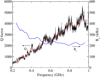
Figure 2: Simulated Q-factor and coherence bandwidth.

III-B Uncorrelated stirrer positions

Referring to the notation of Section I, we compute $N_{\rm eff}$ either through sampling grid of $N_{w}$ spatial points, i.e., the case 1) US–PM, and through a frequency scanning over $N_{f}$ frequency points, i.e., the case 2) US–FM. Figure 3 shows $N_{\rm eff}$ as calculated with $N_{w}=512$ and $N_{f}=512$. The same Figure also reports $N_{\rm eff}$ computed through the standard, i.e., circular correlation (CC), technique as described in the IEC standard [1]. It is worth noticing that the US–PM method underestimates $N_{\rm eff}$ with respect to the CC method. This happens also varying the number of grid spatial points [20] and the number of frequency points [33]. Conversely, the US–FM method overestimates $N_{\rm eff}$. Again, the sampling frequency step is greater than or equal to $B_{c}$. The effect of bandwidth variation was investigated in [7], where a lower number of frequency points were adopted to build up the correlation matrix.

Interestingly, the curve related to US–FM saturates when the cavity coherence bandwidth reaches the sampling frequency, viz.,

$$B_{c}\approx\Delta f=305\mbox{ kHz}\,\,.$$ (10)

Below this frequency, evaluating uncorrelated positions with this strategy mean sampling over $B_{c}$, as shown in Figure 2, whence $B_{c}<\Delta f$ results in $N_{\rm eff}\leq N_{s}$.

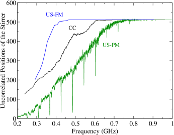
Figure 3: Simulated uncorrelated stirrer positions, for a correlation matrix of grid points (US–PM) and of frequency points (US–FM). Results applying the IEC standard method are also reported (CC).

III-C Uncorrelated frequency points

In those RC applications, where the electronic stirring method is thus employed, it is important to know whether the frequency steps are uncorrelated or not. Figure 4 shows the number of uncorrelated frequencies as calculated in the UF–PM strategy. It is worth pointing out two interesting features. Adopting the total field $|E|$, the frequency points become correlated below 400 MHz, where the frequency step is lower than the chamber $B_{c}$. On the other hand, the single rectangular component gives a lower number of frequency uncorrelation points. Conversely, there is no difference when the uncorrelated stirrer positions are evaluated by $|E|$ or by $E_{x,y,z}$ [20], i.e. in the US–PM strategy. Results refer to a fixed stirrer angle. The gray area in Figure 4 shows the spreading of the uncorrelated frequency points for 16 stirrer positions. This indirectly quantifies the uncertainty of the estimation. Figure 4 shows a very limited spreading.

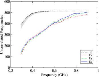
Figure 4: Simulated uncorrelated frequency points for a correlation matrix of grid points (UF–PM). Each component and the magnitude of the electric field are reported. The gray area is the spread for 16 stirrer angles.

The determination of uncorrelated frequency number can also be done populating the correlation matrix with the field values computed in a single chamber point by rotating the stirrer (UF–SM). Figure 5 shows the simulated number of uncorrelated frequencies. A similar behavior to the case UF–PM is observed. The gray area of Figure 5 shows a larger uncertainty than the one in Figure 4.

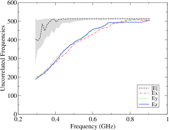
Figure 5: Simulated uncorrelated frequency points for a correlation matrix of stirrer angles (UF–SM). The gray area is the spread for all the 512 grid points.

The discrepancy of Figure 4 and Figure 5 can be ascribed to the nature of modes inside of an RC. The Weyl law quantifies the eigenmode density of an EM cavity, while no information is given on the nature of those eigenmodes.

At relatively low frequencies, the chamber modes (TE and TM) can be still considered unperturbed [1]. At higher frequencies, the modes become hybrid due to the presence of stirrer blades, and all the three Cartesian components are involved in the total field representation. Uncorrelated stirrer positions are not affected by any partitioning since their evaluation involves averaging over space (mode topology) or over frequency (eigenspectrum) of the RC fields.

III-D Random stir sampling

The definition (7) has a straightforward physical meaning: the number of independent positions can be evaluated as the number of stirring configurations having acceptable spatial dispersion of the (Cartesian or total) field variance. Therefore, given a sampling subspace, it is possible to construct a two-position correlation function over a discretized, i.e., tuned, stirrer rotation. The theoretical prediction of $N_{\rm eff}$ based on (7) is not an easy task.

In a very general fashion, we could also treat $r_{i}j$ as a random variable through $\ushortdw{R}_{s,f}$. In this perspective, its probability distribution would be regulated by the space/frequency sampling. Inherently, a randomized sampling over continuous stirrer rotations is more realistic and would naturally call for a statistical treatment of $r_{ij}$, though in principle also in deterministic sampling it is possible to linearize $\ushortdw{R}_{s,f}$, order its elements $r_{ij}$, and calculate the probability density function (PDF) of the correlation as a distribution of its values. Therefore, also $N_{\rm eff}$ becomes a random variable with probability density function $f_{N_{\rm eff}}\left(n_{eff}\right)$. Exploiting the addition theorem in probability, we can turn the probability of the counting operator into a union of probabilities of the single element $f_{R}\left(r<\overline{r}\right)$. Obviously, the ability of obtaining many single uncorrelated elements $r=r_{ij}\leq\overline{r}$ depends on the stirring parameters such as structure geometry, location, and dimensions. The evaluation of the stirring efficiency can be performed deterministically by full-wave numerical simulations or measurements on actual structures. Our perspective calls for a statistical approach to the problem: instead of a pure deterministic evaluation, it would be useful to introduce a probability $f_{R}\left(r<\overline{r}\right)$ of the mode-stirrer to make two arbitrary realizations uncorrelated.

Furthermore, counting $n_{eff}$ positions in $\mathcal{N}_{s}$ elements means having $n_{eff}$ successes with probability $f_{R}\left(r<\overline{r}\right)$ in $\mathcal{N}_{s}$ trials, that is given by the Bernoulli (or binomial) distribution. Assuming uncorrelated elements of the correlation matrix, and a deterministic threshold of $\overline{r}$, yields

$$\begin{split}f_{N_{\rm eff}}\left(n_{eff},\overline{r}\right)=\binom{n_{eff}}{\mathcal{N}_{s}}\,\left[f_{R}\left(r<\overline{r}\right)\right]^{n_{eff}}\\ \left[1-f_{R}\left(r<\overline{r}\right)\right]^{\mathcal{N}_{s}-n_{eff}}\,\,,\end{split}$$ (11)

where the effective number of considered pairs of chamber configurations is given by half the number of off-diagonal elements of the correlation matrix, viz.,

$$\mathcal{N}_{s}=\frac{N_{s}\left(N_{s}-1\right)}{2}\,\,,$$ (12)

and the event probability is actually a cumulative distribution function (CDF)

$$F_{R}\left(\overline{r}\right)=f_{R}\left(r<\overline{r}\right)=\int_{0}^{\overline{r}}\,\,f_{R}\left(r\right)\,\,dr\,\,.$$ (13)

Further physical considerations would be involved in presence of lattice autocorrelation. In this paper we treat the case of uncorrelated sampling space/frequency lattice. Once obtained the distribution of $n_{eff}$, a robust estimation of the number of independent is possible by continuous averaging

$$\overline{N}_{\rm eff}\left(\overline{r}\right)=\int\,\,\delta\left(n_{eff}-n\right)\,f_{N_{\rm eff}}\left(n,\overline{r}\right)\,dn\,\,,$$ (14)

which is given by

$$\overline{N}_{\rm eff}\left(\overline{r}\right)=\mathcal{N}_{s}F_{R}\left(\overline{r}\right)\,\,.$$ (15)

The challenge is now devoted to the derivation of the correlation distribution $f_{R}\left(r\right)$, and to understanding its dependence on chamber and stirrer parameters [21, 34] such as chamber volume and losses. Here, we present distributions the correlation function resulting from numerical (FDTD) data.

The PDF of $f_{R}\left(r\right)$ is reported in Figure 6 for the correlation of the Cartesian field $\left|E_{x}\right|$, as obtained through the US–PM strategy.

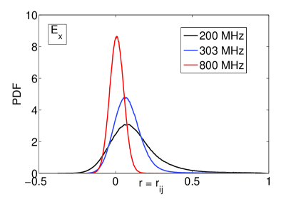
Figure 6: Probability density function of the off-diagonal element of correlation matrix for $\left|E_{x}\right|$ at low (200 MHz), intermediate (303 MHz), and high (800 MHz) frequency, for a spatial grid $13\times 13\times 11$ of the US–PM strategy.

Similar distributions are obtained for the components $E_{y}$ and $E_{z}$. Those are shown in Figure 7 and Figure 8.

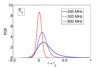
Figure 7: Probability density function of the off-diagonal element of correlation matrix for $\left|E_{y}\right|$ at low (200 MHz), intermediate (303 MHz), and high (800 MHz) frequency, for a spatial grid $13\times 13\times 11$ of the US–PM strategy.

Interestingly, the PDF of $\left|E_{x}\right|$, $\left|E_{y}\right|$, and $\left|E_{z}\right|$ has non-central $t$-student profile. This is consistent with the statistics of two superimposed partially developed speckles in spatial optics [35]. Also, observations confirm isotropic behavior and ergodicity over the investigated frequency range. Furthermore, it looks had to get rid of any residual correlation, whence the importance of fixing a threshold, and the genesis of the uncorrelation seems to be related to the positive tail. This has the important implication of changing the conventional uncorrelation threshold from $\left|r_{ij}\right|<\rho_{e}$ to $r_{ij}<\rho_{e}$.

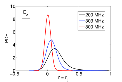
Figure 8: Probability density function of the off-diagonal element of correlation matrix for $\left|E_{z}\right|$ at low (200 MHz), intermediate (303 MHz), and high (800 MHz) frequency, for a spatial grid $13\times 13\times 11$ of the US–PM strategy.

In this perspective, the presence of a threshold is of key importance as it looks that non-central behavior of the correlation PDF at low frequencies creates a fat tail in the region $r_{ij}>e^{-1}$.

In order to speculate more on the importance of a threshold, we present the PDF of the two-position correlation function calculated through the total field $E$. This is reported in Figure 9.

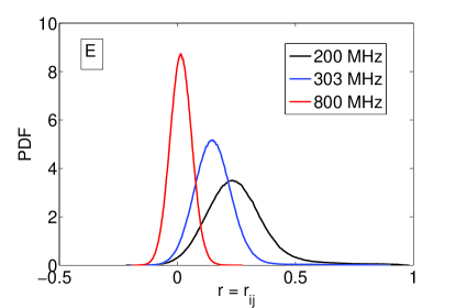
Figure 9: Probability density function of the off-diagonal element of correlation matrix for $\left|E\right|$ at low (200 MHz), intermediate (303 MHz), and high (800 MHz) frequency, for a spatial grid $13\times 13\times 11$ of the US–PM strategy.

Interestingly, we observe that the average value of the non-central $t$-student at low frequency is located where the tail of the high frequency distribution is almost absent. Furthermore, it looks that this average value goes to $e^{-1}$ as the frequency approaches the LUF, $f_{l}$. This suggest the definition of a threshold which is strictly related to the RC under consideration. In particular, the arbitrary choice of a threshold can be turned into a more “physics-based”, or RC based, definition through

$$\overline{r}\approx\lim_{f\rightarrow f_{l}}\,\left<r_{\tau_{i},\tau_{j}}\left(f\right)\right>_{\tau=\tau_{i}-\tau_{j}}\,\,,$$ (16)

with $r_{\tau}$ calculated as the total field correlation over a proper sampling lattice.

III-E Uncorrelated spatial points

Figure 10 shows the simulated the number of uncorrelated grid points for a correlation matrix of stirrer angles (UP–SM). Again, when computed through the total electric field magnitude, this number exhibits higher values with respect to the single components. By using the rectangular components, the adopted grid points are uncorrelated above 800 MHz, where the point distance is $0.4\lambda$. This result is close to the expected spatial correlation length of $0.5\lambda$. By using the total field, the adopted grid points are uncorrelated above 650 MHz, where the point distance is $0.325\lambda$. This could be explained by a consideration similar to that done and the end of Section III-C. The effect of the number of stirrer positions used to compute the correlation matrix is reported in Figure 11. When the number of positions is large enough, the results converge to the same values, while decreasing the number of positions gives rise to lower values. This means that the correlation must be computed over a sufficiently large data ensemble. Moreover, regular frequency peaks where correlation increases appear. These peaks are also visible in the US–PM case and investigated in [20]. They do not depend on the adopted strategy, but on the RC geometry. In particular, peak distance corresponds to a value for which the RC dimension along the stirrer rotation axis is $0.5\lambda$, which is 60 MHz for this RC.

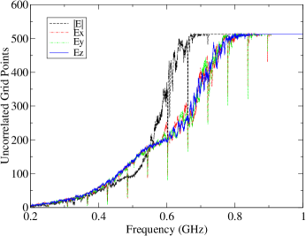
Figure 10: Simulated uncorrelated grid points for a correlation matrix of stirrer positions (UP–SM). Each component and the magnitude of the electric field are reported.

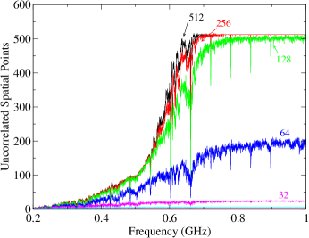
Figure 11: Simulated uncorrelated grid points as function of the number of stirrer positions used in the computation of the correlation matrix (UP–SM). The $|E|$ was used.

Figure 12 shows the simulated number of uncorrelated grid points for the strategy UP–FM. At each working frequency, we compute the correlation coefficients using a set of $N_{f}$ frequency points, which defines the frequency stirring bandwidth $B_{w}$. When we use $N_{f}=512$, $B_{w}=156$ MHz. The effect of the number of stirrer positions on the estimated number of uncorrelated frequencies is reported in Figure 13. The frequency points where the correlation is calculated are the same. All the frequency points are equidistant, therefore reducing $N_{f}$ has the effect of decreasing $B_{w}$. When the number of frequency points is large enough, the results converge. Decreasing $N_{f}$, a reduction of the number of uncorrelated points is observed. In the FM strategies, peaks where uncorrelation decreases are not visible due to the intrinsic frequency averaging of the method.

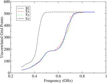
Figure 12: Simulated uncorrelated grid points for a correlation matrix of frequency points (UP–FM). Each component and the magnitude of the electric field are reported.

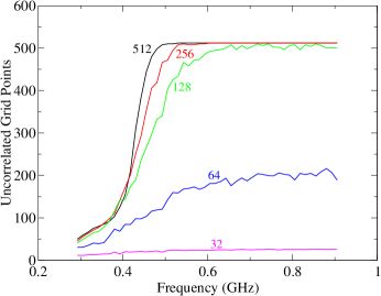
Figure 13: Simulated uncorrelated grid points as function of the number of frequency points used in the computation of the correlation matrix (UP–FM). The $|E|$ was used.

IV Conclusions

We have compared existing methods to estimate the number of uncorrelated stirrer positions through the correlation matrix of multivariate stir traces. An actual reverberation chamber has been simulated through a full wave, finite-difference time-domain parallel code. Spatial and frequency multi-point sampling of stir traces offer an overall picture of the field distributions of the reverberation chamber. A threshold is introduced to count the uncorrelated pairs of stirrer positions. Pertaining this case, we observed that the classical autocorrelation method overestimates the uncorrelated blade positions. Estimation of uncorrelated frequencies and spatial grid points is also possible, which is of interest in frequency and spatial stirring techniques. We noted an overestimation of uncorrelated pairs if frequency samples are used. The use of Cartesian field components underestimate the uncorrelated frequency and space points. Conversely, uncorrelated stirrer positions are not effected by this choice. In general, a sufficiently large date ensemble is necessary to correctly compute the correlation. Finally, the probability density function of the correlation matrix elements has been investigated. The observed frequency evolution (function width and positive tail) suggests a threshold value tailored to the lowest usable frequency of the chamber.

References

- [1] Electromagnetic compatibility (EMC) - Part 4-21: Testing and measurement techniques - Reverberation chamber test methods, 2nd ed., International Standards - IEC 61000-4-21, Geneva, Switzerland, Apr. 2011.
- [2] S. Pfennig and H. G. Krauthäuser, “A general method for determining the number of independent stirrer positions in reverberation chambers,” in 2012 International Symposium on Electromagnetic Compatibility (EMC EUROPE), Sep. 2012, pp. 1–6.
- [3] A. Sorrentino, G. Ferrara, and M. Migliaccio, “On the coherence time control of a continuous mode stirred reverberating chamber,” IEEE Trans. Antennas Propag., vol. 57, no. 10, pp. 3372–3374, Oct. 2009.
- [4] E. Amador, C. Lemoine, and P. Besnier, “Numerical study of spatial correlation in reverberation chamber,” Electronics Letters, vol. 47, no. 24, pp. 1319–1320, 2011.
- [5] X. Chen, “On independent platform sample number for reverberation chamber measurements,” IEEE Trans. Electromagn. Compat., vol. 54, no. 6, pp. 1306–1309, Dec. 2012.
- [6] R. J. Pirkl, “Spatial autocovariances of scattering parameters measured in a lossy reverberation chamber,” IEEE Trans. Electromagn. Compat., vol. 55, no. 4, pp. 671–682, 2013.
- [7] G. Gradoni, V. Mariani Primiani, and F. Moglie, “Reverberation chamber as a multivariate process: FDTD evaluation of correlation matrix and independent positions,” Progress In Electromagnetics Research, vol. 133, pp. 217–234, 2013.
- [8] R. J. Pirkl, K. A. Remley, and C. S. L. Patané, “Reverberation chamber measurement correlation,” IEEE Trans. Electromagn. Compat., vol. 54, no. 3, pp. 533–545, Jun. 2012.
- [9] F. Moglie and V. Mariani Primiani, “Numerical analysis of a new location for the working volume inside a reverberation chamber,” IEEE Trans. Electromagn. Compat., vol. 54, no. 2, pp. 238–245, Apr. 2012.
- [10] U. Dörr, H.-J. Stöckmann, M. Barth, and U. Kuhl, “Scarred and chaotic field distributions in a three-dimensional sinai-microwave resonator,” Phys. Rev. Lett., vol. 80, pp. 1030–1033, Feb 1998.
- [11] J. Barthélemy, O. Legrand, and F. Mortessagne, “Complete s matrix in a microwave cavity at room temperature,” Phys. Rev. E, vol. 71, p. 016205, Jan 2005.
- [12] C. Lemoine, P. Besnier, and M. Drissi, “Investigation of reverberation chamber measurements through high-power goodness-of-fit tests,” IEEE Trans. Electromagn. Compat., vol. 49, no. 4, pp. 745–755, Nov. 2007.
- [13] A. Cozza, “A skeptic’s view of unstirred components,” in EMC Europe 2011 York, York, UK, Sep. 2011, pp. 174–179.
- [14] C. S. Bretherton, M. Widmann, V. P. Dymnikov, J. M. Wallace, and I. Blade, “The effective number of spatial degrees of freedom of a time-varying field,” Journal of Climate, vol. 12, no. 7, pp. 1990–2009, Jul. 1990.
- [15] L. R. Arnaut, “Optimizing low-frequency mode stirring performance using principal component analysis,” IEEE Trans. Electromagn. Compat., vol. 56, no. 1, pp. 3–14, 2014.
- [16] O. M. Bucci and G. Franceschetti, “On the degrees of freedom of scattered fields,” IEEE Trans. Antennas Propag., vol. 37, no. 7, pp. 918–926, Jul. 1989.
- [17] G. Gradoni, V. Mariani Primiani, and F. Moglie, “Reverberation chamber as a statistical relaxation process: Entropy analysis and fast time domain simulations,” in 2012 International Symposium on Electromagnetic Compatibility (EMC EUROPE), Rome, Italy, Sep. 2012, pp. 1–6.
- [18] L. F. Santos, F. Borgonovi, and F. M. Izrailev, “Chaos and statistical relaxation in quantum systems of interacting particles,” Phys. Rev. Lett., vol. 108, p. 094102, Mar. 2012.
- [19] S. Pfennig and H. G. Krauthäuser, “Comparison of methods for determining the number of independent stirrer positions in reverberation chambers,” in 2013 International Symposium on Electromagnetic Compatibility (EMC EUROPE), Brugge Belgium, Sep. 2013, pp. 431–436.
- [20] G. Gradoni, V. Mariani Primiani, and F. Moglie, “Carousel stirrer efficiency evaluation by a volumetric lattice-based correlation matrix,” in 2013 IEEE International Symposium on Electromagnetic Compatibility (EMC), Denver, CO, USA, Aug. 2013, pp. 819–824.
- [21] F. Moglie and V. Mariani Primiani, “Analysis of the independent positions of reverberation chamber stirrers as a function of their operating conditions,” IEEE Trans. Electromagn. Compat., vol. 53, no. 2, pp. 288–295, May 2011.
- [22] S. Mengue, E. Richalot, and O. Picon, “Comparison between different criteria for evaluating reverberation chamber functioning using a 3-D FDTD algorithm,” IEEE Trans. Electromagn. Compat., vol. 50, no. 2, pp. 237–245, May 2008.
- [23] A. Adardour, G. Andrieu, and A. Reineix, “On the low-frequency optimization of reverberation chambers,” IEEE Trans. Electromagn. Compat., vol. 56, no. 2, pp. 266–275, 2014.
- [24] Y. Cui, G. Wei, S. Wang, L. Fan, and Y. Zhao, “Fast analysis of reverberation chamber using FDTD method and matrix pencil method with new criterion for determining the number of exponentially damped sinusoids,” IEEE Trans. Electromagn. Compat., 2014, to be published, DOI: 10.1109/TEMC.2013.2294691.
- [25] V. Mariani Primiani and F. Moglie, “Reverberation chamber performance varying the position of the stirrer rotation axis,” IEEE Trans. Electromagn. Compat., vol. 56, no. 2, pp. 486–489, 2014.
- [26] F. Moglie and V. Mariani Primiani, “Numerical simulations of field values, wave impedance, and received power inside a nonideal reverberation chamber,” IEEE Trans. Electromagn. Compat., 2014, to be published, DOI: 10.1109/TEMC.2013.2290806.
- [27] D. A. Hill, M. T. Ma, A. R. Ondrejka, B. F. Riddle, M. L. Crawford, and R. T. Johnk, “Aperture excitation of electrically large, lossy cavities,” IEEE Trans. Electromagn. Compat., vol. 36, no. 3, pp. 169–178, Aug. 1994.
- [28] X. Chen, P.-S. Kildal, C. Orlenius, and J. Carlsson, “Channel sounding of loaded reverberation chamber for over-the-air testing of wireless devices: Coherence bandwidth versus average mode bandwidth and delay spread,” IEEE Antennas Wireless Propag. Lett., vol. 8, pp. 678–681, 2009.
- [29] O. Delangre, P. De Doncker, M. Lienard, and P. Degauque, “Delay spread and coherence bandwidth in reverberation chamber,” Electronics Letters, vol. 44, no. 5, pp. 328–329, 2008.
- [30] C. L. Holloway, H. A. Shah, R. J. Pirkl, K. A. Remley, D. A. Hill, and J. Ladbury, “Early time behavior in reverberation chambers and its effect on the relationships between coherence bandwidth, chamber decay time, RMS delay spread, and the chamber buildup time,” IEEE Trans. Electromagn. Compat., vol. 54, no. 4, pp. 714–725, Aug. 2012.
- [31] L. R. Arnaut, “Operation of electromagnetic reverberation chambers with wave diffractors at relatively low frequencies,” IEEE Trans. Electromagn. Compat., vol. 43, no. 4, pp. 637–653, Nov. 2001.
- [32] A. Cozza, “The role of losses in the definition of the overmoded condition for reverberation chambers and their statistics,” IEEE Trans. Electromagn. Compat., vol. 53, no. 2, pp. 296–307, May 2011.
- [33] G. Gradoni, V. Mariani Primiani, and F. Moglie, “Determination of the reverberation chamber stirrer uncorrelated positions by means of the spatial and frequency correlation matrix,” in 2013 International Symposium on Electromagnetic Compatibility (EMC EUROPE), Brugge Belgium, Sep. 2013, pp. 425–430.
- [34] V. Mariani Primiani and F. Moglie, “Numerical simulation of reverberation chamber parameters affecting the received power statistics,” IEEE Trans. Electromagn. Compat., vol. 54, no. 3, pp. 522–532, Jun. 2012.
- [35] N. Yaitskova, “Probability density function and detection threshold in high contrast imaging with partially polarized light,” Optics letters, vol. 34, no. 11, pp. 1720–1722, 2009.