Automated adaptive inference of coarse-grained dynamical models in systems biology

Abstract

Cellular regulatory dynamics is driven by large and intricate networks of interactions at the molecular scale, whose sheer size obfuscates understanding. In light of limited experimental data, many parameters of such dynamics are unknown, and thus models built on the detailed, mechanistic viewpoint overfit and are not predictive. At the other extreme, simple ad hoc models of complex processes often miss defining features of the underlying systems. Here we propose an approach that instead constructs phenomenological, coarse-grained models of network dynamics that automatically adapt their complexity to the amount of available data. Such adaptive models lead to accurate predictions even when microscopic details of the studied systems are unknown due to insufficient data. The approach is computationally tractable, even for a relatively large number of dynamical variables, allowing its software realization, named Sir Isaac, to make successful predictions even when important dynamic variables are unobserved. For example, it matches the known phase space structure for simulated planetary motion data, avoids overfitting in a complex biological signaling system, and produces accurate predictions for a yeast glycolysis model with only tens of data points and over half of the interacting species unobserved.

^∗E-mail: bdaniels@discovery.wisc.edu, ilya.nemenman@emory.edu

I Introduction

Systems biology is a field of complicated models — and rightfully so: the vast amount of experimental data has clearly demonstrated that cellular networks have a degree of complexity that is far greater than what is normally encountered in the physical world (Hlavacek:2009kf). Mathematical models of these data are often as complicated as the data themselves, reflecting the humorous maxim that “the best material model of a cat is another, or preferably the same, cat” (Rosenblueth:1945tz). However, continued success of approaches that systematize all known details in a combinatorially large mathematical model is uncertain. Indeed, generalizing and generating insight from complex models is difficult. Further, specification of myriads of microscopic mechanistic parameters in such models demands vast data sets and computational resources, and sometimes is impossible even from very large data sets due to widely varying sensitivities of predictions to the parameters (Gutenkunst:2007gl). Finally, the very structures of these models are often unknown because they depend on many yet-unobserved players on the cellular, molecular, and sub-molecular levels. Identification of these structural characteristics of the involved processes is labor intensive and does not scale up easily. With these challenges, it is unlikely that mathematical models based solely on a reductionist representation will be able to account accurately for the observed dynamics of cellular networks. More importantly, even if they could, the resulting models would be too unwieldy to bring about understanding of the modeled systems.

Because of these difficulties, the need to use systems biology data to predict responses of biological systems to dynamical perturbations, such as drugs or disease agents, has led to a resurgence of research into automated inference of dynamical systems from time series data, which had been attempted since the early days of the field of nonlinear dynamics (Crutchfield:1987va; PacCruFar80). Similar needs in other data-rich fields in natural and social sciences and engineering have resulted in successful algorithms for distilling continuous dynamics from time series data, using approaches such as linear dynamic models (FriHarPen03), recurrent neural networks (SusAbb09), evolved regulatory networks (FraHakSig07), and symbolic regression (Schmidt:2009dt; SchValJen11). The latter two approaches produce models that are more mechanistically interpretable in that they incorporate nonlinear interactions that are common in systems biology, and they actively prune unnecessary complexity. Yet these approaches are limited because, in a search through all possible microscopic dynamics, computational effort typically explodes with the growing number of dynamical variables. In general, this leads to very long search times (FraHakSig07; SchValJen11), especially if some underlying variables are unobserved, and dynamics are coupled and cannot be inferred one variable at a time.

To move forward, we note that, while biological networks are complex, they often realize rather simple input-output relations, at least in typical experimental setups. Indeed, activation dynamics of a combinatorially complex receptor can be specified with only a handful of large-scale parameters, including the dynamic range, cooperativity, and time delay (Goldstein:2004ch; Bel:2010er; Cheong:2011jp). Also, some microscopic structural complexity arises in order to guarantee that the macroscopic functional output remains simple and robust in the face of various perturbations (Bel:2010er; Lander:2011bj). Thus one can hope that macroscopic prediction does not require microscopic accuracy (MacChaTra13), and hence seek phenomenological, coarse-grained models of cellular processes that are simple, inferable, and interpretable, and nonetheless useful in limited domains.

In this report, we propose an adaptive approach for dynamical inference that does not attempt to find the single best microscopically “correct” model, but rather a phenomenological model that remains mechanistically interpretable and is “as simple as possible, but not simpler” than needed to account for the experimental data. Relaxing the requirement for microscopic accuracy means that we do not have to search through all possible microscopic dynamics, and we instead restrict our search to a much smaller hierarchy of models. By choosing a hierarchy that is nested and complete, we gain theoretical guarantees of statistical consistency, meaning the approach is able to adaptively fit any smooth dynamics with enough data, yet is able to avoid problems with overfitting that can happen without restrictions on the search space (Nem05). While similar complexity control methods are well established in statistical inference (MacKay:2003wc), we believe that they have not been used yet in the context of inferring complex, nonlinear dynamics. Importantly, this adaptive approach is typically much more efficient because there are far fewer models to test. Instead of searching a super-exponentially large model space (Schmidt:2009dt), our method tests a number of models that scales polynomially with the number of dynamical variables. Further, it uses computational resources that asymptotically scale linearly with the number of observations. This allows us to construct interpretable models with much smaller computational effort and fewer experimental measurements, even when many dynamical variables are unobserved. We call the approach Sir Isaac due to its success in discovering the law of universal gravity from simulated data (see below).

II Methods and Results

II.1 Classes of phenomenological models used by Sir Isaac

We are seeking a phenomenological model of dynamics in the form

$$\frac{d\vec{x}}{dt}=\vec{F_{x}}(\vec{x},\vec{y},\vec{I}),~{}~{}\frac{d\vec{y}}{dt}=\vec{F_{y}}(\vec{x},\vec{y},\vec{I}),$$ (1)

where $\vec{x}$ are the observed variables, $\vec{y}$ are the hidden variables, and $\vec{I}$ are the inputs or other parameters to the dynamics. We neglect intrinsic stochasticity in the dynamics (either deterministic chaotic, or random thermal), and focus on systems where repeated observations with nearly the same initial conditions produce nearly the same time series, save for measurement noise. The goal is then to find a phenomenological model of the force fields $\vec{F}_{x},\vec{F}_{y}$ (Crutchfield:1987va). The same dynamics may produce different classes of trajectories $\vec{x}(t)$ dependent on initial conditions (e. g., elliptical vs. hyperbolic trajectories in gravitational motion). Thus the focus on dynamical inference rather than on more familiar statistical modeling of trajectories allows the representation of multiple functional forms within a single dynamical system.

To create a model, we would like to gradually increase the complexity of $F$ until we find the best tradeoff between good fit and sufficient robustness, essentially extending traditional Bayesian model selection techniques to the realm of dynamical models. Ideally, this process should progress much like a Taylor series approximation to a function, adding terms one at a time in a hierarchy from simple to more complex, until a desired performance is obtained. To guarantee that this is possible, the hierarchy of models must be nested (or ordered) and complete in the sense that any possible dynamics can be represented within the hierarchy (Nem05) (see Supplementary Online Materials (SOM)). Any model hierarchy that fits these criteria may be used, but ordering dynamical models that can be made more complex along two dimensions (by adding either nonlinearities or unobserved variables) is nontrivial. Further, different model hierarchies may naturally perform differently on the same data, depending on whether the studied dynamics can be represented succinctly within a hierarchy.

We construct two classes of nested and complete model hierarchies, both well matched to properties of biochemistry that underlies cellular network dynamics. We build the first with S-systems (SavVoi87) and the second with continuous time sigmoidal networks (Bee06) (see SOM). The S-systems use production and degradation terms for each dynamical variable formed by products of powers of species concentrations; this is a natural generalization of biochemical mass-action laws. The sigmoidal class represents interactions using linear combinations of saturating functions of species concentrations, similar to saturation in biochemical reaction rates. Both classes are complete and are able to represent any smooth dynamics with a sufficient number of (hidden) dynamical variables (SavVoi87; FunNak93; ChoLi00). It is possible that both classes can be unified into power-law dynamical systems with algebraic power-law constraints among the dynamical variables (SavVoi87), but this will not be explored in this report.

II.2 Description of model selection procedure

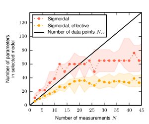
To perform adaptive fitting within a model class, a specific ordered hierarchy of models is chosen a priori that simultaneously varies both the degree of nonlinearity and the number of hidden variables (see FIG. S1 and SOM). For each model in the hierarchy, its parameters are fit to the data and an estimate of the Bayesian log-likelihood $\mathcal{L}$ of the model is calculated. This estimate makes use of a generalized version of the Bayesian Information Criterion (Sch78), which we have adopted, for the first time, for use with nonlinear dynamical systems inference. As models increase in complexity, $\mathcal{L}$ first grows as the quality of fit increases, but eventually begins to decrease, signifying overfitting. Since, statistical fluctuations aside, there is just one peak in $\mathcal{L}$ (Nem05), one can be certain that the global maximum has been observed once it has decreased sufficiently. The search through the hierarchy is then stopped, and the model with maximum $\mathcal{L}$ is “selected” (see FIG. 4(b)).

II.3 The law of gravity

Figure 1: The law of gravity: an example of dynamical inference. A particle is released with velocity $v_{0}$ perpendicular to the line connecting it to the sun, with varying initial distance $r_{0}$ from the sun. (a) With only $N=150$ examples (each consisting of just a single noisy observation of $r$ at a random time $t$ after the release; see SOM), we infer a single dynamical model in the S-systems class that reproduces the data. With no supervision, adaptive dynamical inference produces bifurcations that lead to qualitatively different behavior: in this case, a single model produces both oscillations (corresponding to elliptical orbits) and monotonic growth (corresponding to hyperbolic trajectories). Inferred trajectories are shown with solid colored lines, and the corresponding true trajectories are shown with dashed lines. (b) Like the true model (left), the inferred model (right) contains a single hidden variable $X_{2}$ and works using a similar phase space structure. Specifically, the location of nullclines (green lines) and a single fixed point (green circle) as a function of $r_{0}$ are recovered well by the fit. Note that the hidden variable is defined up to a power (see SOM), and we choose to plot $X^{2}_{2}$ here.

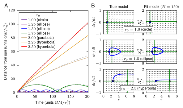
Before applying the approach to complex biological dynamics, where the true model may not be expressible simply within the chosen search hierarchy, we test it on a simpler system with a known exact solution. We choose the iconic law of gravity, inferred by Newton based on empirical observations of trajectories of planets, the Moon, and, apocryphally, a falling apple. Crucially, the inverse-squared-distance law of Newtonian gravity can be represented exactly within the S-systems power-law hierarchy for elliptical and hyperbolic trajectories, which do not go to zero radius in finite time. It requires a hidden parameter, the velocity, to completely specify the dynamics of the distance of an object from the sun (see SOM for specification of the model).

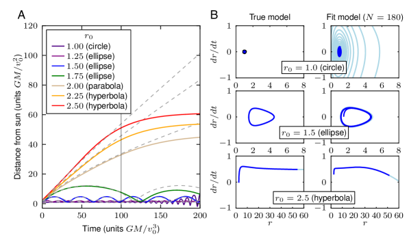
FIG. 1 displays the result of the adaptive inference using the S-systems class. When given data about distance of an object from the sun over time, we discover a model that reproduces the underlying dynamics, including the necessary hidden variable and the bifurcation points. Since the trajectories include hyperbolas and ellipses, this example emphasizes the importance of inferring a single set of dynamical equations of motion, rather than statistical fits to trajectories themselves, which would be different for the two cases. FIG. S3 additionally shows fits for the law of gravity using the sigmoidal models class. While accurate, the fits are worse than those for the S-systems, illustrating importance of understanding of basic properties of the studied system when approaching automated model inference.

Empowered by the success of the adaptive inference approach for this problem, we chose to name it Sir Isaac. The software implementation can be found under the same name on GitHub.

II.4 Multi-site phosphorylation model

When inferring models for more general systems, we do not expect the true dynamics to be perfectly representable by any specific model class: even the simplest biological phenomena may involve combinatorially many interacting components. Yet for simple macroscopic behavior, we expect to be able to use a simple approximate model that can produce useful predictions. To demonstrate this, we envision a single immune receptor with $n$ modification sites, which can exist in $2^{n}$ microscopic states (HlaFaeBli06), yet has simple macroscopic behavior for many underlying parameter combinations. Here, we test a model receptor that can be phosphorylated at each of $n=5$ sites arranged in a linear chain. The rates of phosphorylation and dephosphorylation at each site are affected by the phosphorylation states of its nearest neighboring sites. This produces a complicated model with 32 coupled ODEs specified by 52 parameters, which we assume are unknown to the experimenter.

We imagine an experimental setup in which we can control one of these parameters, and we are interested in its effects on the time evolution of the total phosphorylation of all 5 sites. Here, we treat as input $I$ the maximum rate of cooperative phosphorylation of site 2 due to site 3 being occupied, $V$, and measure the resulting time course of total phosphorylation starting from the unphosphorylated state. Experimental measurements are corrupted with noise at the scale of 10% of their values (SOM).

Figure 2: Multi-site phosphorylation model selection as a function of the number of measurements $N$. The sizes of errors made by three models decrease as the amount of data increases. Adaptive sigmoidal models perform roughly as well as a custom-made simple 5-parameter model for small $N$, but outperform the simple model for large amounts of data. Although we expect that it will eventually outperform all other models as $N\rightarrow\infty$, a maximum likelihood fit to the full 52-parameter model (dark blue) performs worse in this range of $N$. The mean over 10 sets of input data are shown, with shaded regions indicating the standard deviation of the mean. On the right axis, the number of parameters in each model is indicated, with the sigmoidal model adapting to use more parameters when given more data (red squares).

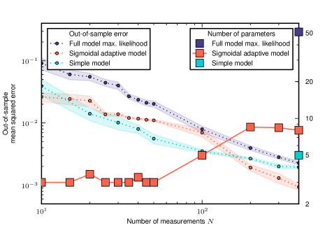
A straightforward approach to modeling this system is to fit the 52 parameters of the known model to the phosphorylation data. A second approach is to rely on intuition to manually develop a functional parameterization that captures the most salient features of the timecourse data. In this case, a simple 5 parameter model (see SOM) captures exponential saturation in time with an asymptotic value that depends sigmoidally on the input $V$. A third approach, advocated here, is to use automated model selection to create a model with complexity that matches the amount and precision of the available data.

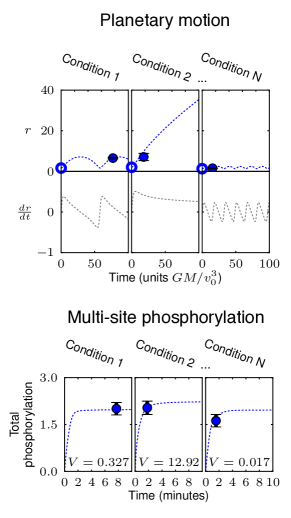
In FIG. 2, we compare these three approaches as the amount of available data is varied, and FIG. 3(a) shows samples of fits done by different procedures. With limited and noisy data, fitting the parameters of the full known model risks overfitting, and in the regime we test, it is the worst performer on out-of-sample predictions. The simple model performs best when fitting to less than 100 data points, but for larger amounts of data it saturates in performance, as it cannot fit more subtle effects in the data. In contrast, an adaptive model remains simple with limited data and then grows to accommodate more subtle behaviors once enough data is available, eventually outperforming the simple model.

Figure 3: Response (right axis) to (a) out-of-sample constant and (b) time-varying input (left axis) in the models of multi-site phosphorylation. Fit to $N=300$ constant input data points, the full known model (dark blue) produces erratic behavior typical of overfitting, while the adaptive sigmoidal model (red) produces more stable out-of-sample predictions with median behavior that is closer to the true dynamics. Dark lines indicate the median behavior over 100 samples from each model’s parameter posterior (see SOM), and shaded regions indicate 90% confidence intervals.

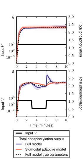
The multi-site phosphorylation example also demonstrates that dynamical phenomenological models found by Sir Isaac are more than fits to the existing data, but rather they uncover the true nature of the system in a precise sense: they can be used to make predictions of model responses to some classes of inputs that are qualitatively different from those used in the inference. For example, as seen in FIG. 3(b), an adaptive sigmoidal model inferred using temporally constant signals produces a reasonable extrapolated prediction for response to a time-varying signal. At the same time, overfitting is evident when using the full, detailed model, even when one averages the model responses over the posterior distribution of the inferred model parameters.

II.5 Yeast glycolysis model

A more complicated system, for which there has been recent interest in automated inference, is the oscillatory dynamics of yeast glycolysis (SchValJen11). A recent model for the system (WolHei00; RuoChrWol03), informed by detailed knowledge of cellular metabolic pathways, consists of coupled ODEs for 7 species with concentrations that oscillate with a period of about 1 minute. The system dynamic is simpler than its structure in the sense that some of the complexity is used to stabilize the oscillations to external perturbations. On the other hand, the oscillations are not smooth (see FIG. 4) and hence are hard to fit with simple methods. These considerations make this model an ideal next test case for phenomenological inference with Sir Isaac.

Figure 4: An example of the model selection process using measurements of timecourses of three metabolites in yeast glycolysis as their initial concentrations are varied. (a) For each set of initial conditions (open circles), a noisy measurement of the three observable concentrations (filled circles) is made at a single random time. Hidden variables (in gray) are not measured. In this example, we fit to $N=40$ in-sample conditions. (b) Models from an ordered class, with the illustrated connectivity, are fit and tested sequentially until $\mathcal{L}$, an approximation of the relative log-likelihood, decreases sufficiently from a maximum. (c) The selected model (large connectivity diagram) is used to make predictions about out-of-sample conditions. Here, we compare the output of the selected model (solid lines) to that of the model that created the synthetic data (dashed lines). (d) Performance versus computational and experimental effort. The mean out-of-sample correlation for 3 measured biochemical species from the range of initial conditions twice that used in training rises to over 0.6 using less than $5\times 10^{8}$ model evaluations and 40 in-sample measurements. In Ref. (SchValJen11), inferring an exact match to the original 7-dimensional model used roughly 500 times as many measurements of all 7 species (with none hidden), which were chosen carefully to be informative. The approach also uses 200 times as many model evaluations (see SOM). Nonetheless, the accuracy of both approaches is comparable, and Sir Isaac additionally retains information about the phase of the oscillations.

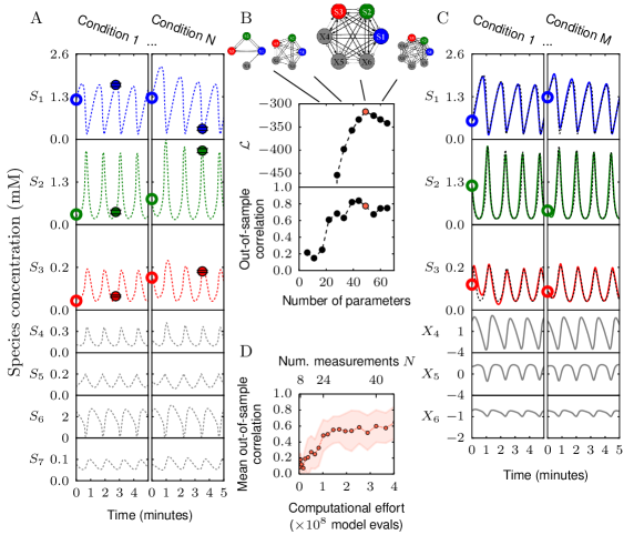
If we were given abundant time series data from all 7 species and were confident that there were no other important hidden species, we may be in a position to infer a “true” model detailing interactions among them. If we are instead in the common situation of having limited data on a limited number of species, we may more modestly attempt to make predictions about the types of inputs and outputs that we have measured. This is conceptually harder since an unknown number of hidden variables may need to be introduced to account for the dynamics of the observed species. We demonstrate our approach by constructing adaptive models of the dynamics from data for only 3 of the 7 coupled chemical species, as their initial conditions are varied.

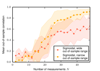
Depicted in FIG. 4 is the model selection procedure for this case. After selecting an adaptive model fit to noisy data from $N$ single timepoints, each starting from initial conditions sampled from specified ranges, we test the inferred model’s ability to predict the timecourse resulting from out-of-sample initial conditions. With data from only $N=40$ measurements, the selected model is able to predict behavior with mean correlation of over 0.6 for initial conditions chosen from ranges twice as large as those used as training data (shown in FIG. 4) and 0.9 for out-of-sample ranges equal to in-sample ranges (shown in FIG. S6). Previous work that inferred the exact equations of the original 7-dimensional model (SchValJen11) used roughly 500 times as many measurements of all 7 variables and 200 times as many model evaluations. This example also demonstrates that adaptive modeling can hint at the complexity of the hidden dynamics beyond those measured: the best performing sigmoidal model requires three hidden variables, for a total of six chemical species — only one less than the true model. Crucially, the computational complexity of Sir Isaac still scales linearly with the number of observations, even when a large fraction of variables remains hidden (see SOM and FIG. S7).

III Discussion

The three examples demonstrate the power of the adaptive, phenomenological modeling approach. Sir Isaac models are inferred without an exponentially complex search over model space, which would be impossible for systems with many variables. These dynamical models are as simple or complex as warranted by data and are guaranteed not to overfit even for small data sets. Thus they require orders of magnitude less data and computational resources to achieve the same predictive accuracy as more traditional methods that infer a pre-defined, large number of mechanistic parameters in the true model describing the system.

These advantages require that the inferred models are phenomenological, and are designed for efficiently predicting the system dynamics at a given scale, determined by the available data. While FIG. 1 shows that Sir Isaac will infer the true model if it falls within the searched model hierarchy, and enough data is available, more generally, the inferred dynamics may be quite distinct from the true microscopic, mechanistic processes, as shown by a different number of chemical species in the true and the inferred dynamics in FIG. 4. What is then the utility of the approach if it says little about the underlying mechanisms?

First, there is the obvious advantage of being able to predict responses of systems to yet-unseen experimental conditions, including those qualitatively different from the ones used for inference. Second, some general mechanisms, such as the necessity of feedback loops or hidden variables, are easily uncovered even in phenomenological models. However, more importantly, we draw the following analogy. When in the 17th century Robert Hooke studied the force-extension relations for springs, a linear model of the relation for a specific spring did not tell much about the mechanisms of force generation. However, the observation that all springs exhibit such linear relations for small extensions allowed him to combine the models into a law — Hooke’s law, the first of many phenomenological physical laws that followed. It instantly became clear that experimentally measuring just one parameter, the Hookean stiffness, provided an exceptionally precise description of the spring’s behavior. And yet the mechanistic understanding of how this Hooke’s constant is related to atomic interactions within materials is only now starting to emerge. Similarly, by studying related phenomena across complex biological systems (e.g., chemotactic behavior in E. coli (Berg:2004wy) and C. elegans (Ryu02), or behavioral bet hedging, which can be done by a single cell (Kussell:2005dg) or a behaving rodent (Gallistel:2001wi)), we hope to build enough models of specific systems, so that general laws describing how nature implements them become apparent.

If successful, our search for phenomenological, emergent dynamics should allay some of the most important skepticism regarding the utility of automated dynamical systems inference in science (Anderson:2009kc), namely that such methods typically start with known variables of interest and known underlying physical laws, and hence cannot do transformative science and find new laws of nature. Indeed, we demonstrated that, for truly successful predictions, the model class used for automated phenomenological inference must match basic properties of the studied dynamics (contrast, for example, FIG. 1 to FIG. S3, and see FIG. S4). Thus fundamental understanding of some key properties of the underlying mechanisms, such as the power-law structure of the law of gravity, or the saturation of biochemical kinetic rates, can be inferred from data even if unknown a priori. Finally, we can contrast our approach with a standard procedure for producing coarse-grained descriptions of inanimate systems: starting from a mechanistically accurate description of the dynamics, and then mapping them onto one of a small set of universality classes (Wilson; MacChaTra13). This procedure is possible due to symmetries of physical interactions that are not typically present in living systems. Without such symmetries, the power of universality is diminished, and microscopic models may result in similarly different macroscopic ones. Then specifying the microscopic model first in order to coarse-grain it later becomes an example of solving a harder problem to solve a simpler one (Vapnik). Thus for living systems, the direct inference of phenomenological dynamics, such as done by Sir Isaac, may be the optimal way to proceed.

Supplementary Materials

S.1 Materials and Methods

S.1.1 Hierarchical Bayesian model selection

For consistent inference, we need a hierarchy of models that satisfies criteria laid out in Ref. (Nem05). First, we desire a model hierarchy that will produce a single maximum in $\mathcal{L}$, up to statistical fluctuations, as we add complexity. For this, the hierarchy should be nested (but not necessarily regular or self-similar), meaning that once a part of the model is added, it is never taken away. Second, the hierarchy should be complete, meaning it is able to fit any data arbitrarily well with a sufficiently complex model. Intuitively, instead of searching a large multidimensional space of models, hierarchical model selection follows a single predefined path through model space (FIG. S1). While the predefined path may be suboptimal for a particular instance (that is, the true model may not fall on it), even then the completeness guarantees that we will still eventually learn any dynamical system $F$ given enough data, and nestedness assures that this will be done without overfitting along the way.

S.1.2 Adaptive model classes and hierarchies

Our first model class is the S-system power-law class. The general form of the S-system representation consists of $J$ dynamical variables $x_{i}$ and $K$ inputs $I_{k}=x_{J+k}$, with each dynamical variable governed by an ordinary differential equation: (SavVoi87)

$$\frac{dx_{i}}{dt}=G(\mathbf{x})_{i}-H(\mathbf{x})_{i},$$ (S1)

with production $G$ and degradation $H$ of the form

$$G(\mathbf{x})_{i} = \alpha_{i}\prod_{j=1}^{J+K}x_{j}^{g_{ij}}$$ (S2)

$$H(\mathbf{x})_{i} = \beta_{i}\prod_{j=1}^{J+K}x_{j}^{h_{ij}}.$$ (S3)

In a process called “recasting,” any set of differential equations written in terms of elementary functions can be rewritten in the power-law form by defining new dynamical variables in the correct way (SavVoi87). Since any sufficiently smooth function can be represented in terms of a series of elementary functions (e. g., Taylor series), a power-law network of sufficient size can describe any such deterministic dynamical system. Note that, since exponents are not constrained to be positive or integer-valued, dynamics in this class are generally ill-defined when variables are not positive.

Figure S1: Hierarchical model selection follows a single predefined path through model space.

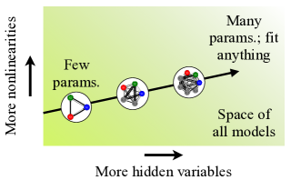
We find that the S-systems model class works well for planetary motion, which has an exact representation in the class; see Section S.1.3. For our biological test examples, the S-systems class is outperformed by the sigmoidal class (see below). This may be indicating that behavior common in the S-systems class is not common in typical biological systems (e. g., real production and degradation terms cannot grow without bounds). It may also stem from the positivity constraint: since the condition that variables remain positive is not easily determined from parameter values, we are forced in our model selection process to simply discard any tested parameters that lead to zero or negative values.

The second model hierarchy is the sigmoidal network class. In this class, we use the fact that the interactions among biological components often take the form of a sigmoidal function to define the following system of ODEs:

$$\frac{dx_{i}}{dt}=-x_{i}/\tau_{i}+\sum_{j=1}^{J}W_{ij}~{}\xi(x_{j}+\theta_{j})+\sum_{k=1}^{N_{p}}V_{ik}I_{k},$$ (S4)

where the sigmoidal function $\xi(y)=1/(1+e^{y})$. This class of models has also been shown to approximate any smooth dynamics arbitrarily well with a sufficient number of dynamical variables (Bee06; BeeDan10; FunNak93; ChoLi00). Note that natural variations of this class to be explored in future work include rescaling of the arguments of the sigmoids $\xi$ or switching the order of operations to apply the sigmoidal function to a linear combination of state variables in order to more closely match traditional neural network models (RumHinWil86).

An advantage of the S-systems and sigmoidal representations is the existence of a natural scheme for creating a one-dimensional model hierarchy: simply adding dynamical variables $x_{i}$. The most general network is fully connected, such that every variable $x_{i}$ has an interaction term in every other $dx_{j}/dt$. Our hierarchy starts with a fully-connected network consisting of the necessary number of input and output variables, and adds “hidden” dynamical variables to add complexity. With each additional $x_{i}$, we add parameters in a predetermined order.

In the S-systems class, without connections, variable $x_{i}$’s behavior is specified by 5 parameters: $x_{i}^{\rm init},\alpha_{i},\beta_{i},g_{ii}$, and $h_{ii}$. Each connection to and from $x_{j}$ is specified by 4 parameters: $g_{ij},g_{ji},h_{ij},$ and $h_{ji}$. When adding a new dynamic variable, we first fix its parameters (to zero for the exponential parameters and one for the multiplicative parameters), and then allow them to vary one at a time in the following order: $g_{ii},g_{ji},h_{ji},g_{ij},h_{ij},\beta_{i},h_{ii},\alpha_{i}$ (adding connections to every other $x_{j}$ one at a time). An example is shown in Table S1.

Model No. $i$	Num. parameters $N_{p}$	Form of power-law ODEs
0	3	$\begin{aligned} x_{1}(0)&=x_{1}^{\rm init}\\ \frac{dx_{1}}{dt}&=x_{I}^{g_{10}}x_{1}^{g_{11}}-\beta_{1}\end{aligned}$
1	4	$\begin{aligned} x_{1}(0)&=x_{1}^{\rm init}\\ \frac{dx_{1}}{dt}&=x_{I}^{g_{10}}x_{1}^{g_{11}}-\beta_{1}x_{I}^{h_{10}}\end{aligned}$
2	5	$\begin{aligned} x_{1}(0)&=x_{1}^{\rm init}\\ \frac{dx_{1}}{dt}&=x_{I}^{g_{10}}x_{1}^{g_{11}}-\beta_{1}x_{I}^{h_{10}}x_{1}^{h_{11}}\end{aligned}$
3	6	$\begin{aligned} x_{1}(0)&=x_{1}^{\rm init}\\ \frac{dx_{1}}{dt}&=\alpha_{1}x_{I}^{g_{10}}x_{1}^{g_{11}}-\beta_{1}x_{I}^{h_{10}}x_{1}^{h_{11}}\\ \end{aligned}$
4	8	$\begin{aligned} x_{1}(0)&=x_{1}^{\rm init}\\ x_{2}(0)&=x_{2}^{\rm init}\\ \frac{dx_{1}}{dt}&=\alpha_{1}x_{I}^{g_{10}}x_{1}^{g_{11}}x_{2}^{g_{12}}-\beta_{1}x_{I}^{h_{10}}x_{1}^{h_{11}}\\ \frac{dx_{2}}{dt}&=x_{2}^{g_{22}}-1\end{aligned}$
5	9	$\begin{aligned} x_{1}(0)&=x_{1}^{\rm init}\\ x_{2}(0)&=x_{2}^{\rm init}\\ \frac{dx_{1}}{dt}&=\alpha_{1}x_{I}^{g_{10}}x_{1}^{g_{11}}x_{2}^{g_{12}}-\beta_{1}x_{I}^{h_{10}}x_{1}^{h_{11}}x_{2}^{h_{12}}\\ \frac{dx_{2}}{dt}&=x_{2}^{g_{22}}-1\end{aligned}$
6	10	$\begin{aligned} x_{1}(0)&=x_{1}^{\rm init}\\ x_{2}(0)&=x_{2}^{\rm init}\\ \frac{dx_{1}}{dt}&=\alpha_{1}x_{I}^{g_{10}}x_{1}^{g_{11}}x_{2}^{g_{12}}-\beta_{1}x_{I}^{h_{10}}x_{1}^{h_{11}}x_{2}^{h_{12}}\\ \frac{dx_{2}}{dt}&=x_{1}^{g_{21}}x_{2}^{g_{22}}-1\end{aligned}$

Table S1: The first seven models of an example hierarchy in the S-systems class with one input $x_{I}$ and fixed initial conditions $x_{1}^{\rm init}$ and $x_{2}^{\rm init}$.

The sigmoidal class is similar: without connections, variable $x_{i}$’s behavior is specified by 4 parameters: $x_{i}^{init},W_{ii},\tau_{i}$, and $\theta_{i}$. Each connection to and from $x_{j}$ is specified by 2 parameters: $W_{ij}$ and $W_{ji}$. When adding a new dynamic variable, we first fix its parameters (to zero for $W$ and $\theta$ and one for $\tau$), and then allow them to vary one at a time in the following order: $W_{ij},W_{ji},W_{ii},\tau_{i},\theta_{i}$ (adding connections to every other $x_{j}$ one at a time). An example is shown in Table S2.

Model No. $i$	Num. parameters $N_{p}$	Form of sigmoidal ODEs
0	3	$\begin{aligned} x_{1}(0)&=x_{1}^{\rm init}\\ \frac{dx_{1}}{dt}&=-x_{1}/\tau_{1}+W_{11}\xi(x_{1})+W_{10}x_{I}\end{aligned}$
1	4	$\begin{aligned} x_{1}(0)&=x_{1}^{\rm init}\\ \frac{dx_{1}}{dt}&=-x_{1}/\tau_{1}+W_{11}\xi(x_{1}+\theta_{1})+W_{10}x_{I}\end{aligned}$
2	6	$\begin{aligned} x_{1}(0)&=x_{1}^{\rm init}\\ x_{2}(0)&=x_{2}^{\rm init}\\ \frac{dx_{1}}{dt}&=-x_{1}/\tau_{1}+W_{11}\xi(x_{1}+\theta_{1})+W_{12}\xi(x_{2})+W_{10}x_{I}\\ \frac{dx_{2}}{dt}&=-x_{2}\end{aligned}$
3	7	$\begin{aligned} x_{1}(0)&=x_{1}^{\rm init}\\ x_{2}(0)&=x_{2}^{\rm init}\\ \frac{dx_{1}}{dt}&=-x_{1}/\tau_{1}+W_{11}\xi(x_{1}+\theta_{1})+W_{12}\xi(x_{2})+W_{10}x_{I}\\ \frac{dx_{2}}{dt}&=-x_{2}+W_{20}x_{I}\end{aligned}$
4	8	$\begin{aligned} x_{1}(0)&=x_{1}^{\rm init}\\ x_{2}(0)&=x_{2}^{\rm init}\\ \frac{dx_{1}}{dt}&=-x_{1}/\tau_{1}+W_{11}\xi(x_{1}+\theta_{1})+W_{12}\xi(x_{2})+W_{10}x_{I}\\ \frac{dx_{2}}{dt}&=-x_{2}+W_{21}\xi(x_{1}+\theta_{1})+W_{20}x_{I}\end{aligned}$
5	9	$\begin{aligned} x_{1}(0)&=x_{1}^{\rm init}\\ x_{2}(0)&=x_{2}^{\rm init}\\ \frac{dx_{1}}{dt}&=-x_{1}/\tau_{1}+W_{11}\xi(x_{1}+\theta_{1})+W_{12}\xi(x_{2})+W_{10}x_{I}\\ \frac{dx_{2}}{dt}&=-x_{2}+W_{22}\xi(x_{2})+W_{21}\xi(x_{1}+\theta_{1})+W_{20}x_{I}\end{aligned}$

Table S2: The first six models of an example model hierarchy in the sigmoidal class with one input $x_{I}$ and fixed $x_{1}^{\rm init}$ and $x_{2}^{\rm init}$.

For every adaptive fit model and the full multi-site phosphorylation model, we use the same prior for every parameter $\alpha_{k}$, which we choose as a normal distribution ${\mathcal{N}}(0,10^{2})$ with mean 0 and standard deviation $\varsigma=10$.

S.1.3 The law of gravity model

For a mass $m$ in motion under the influence of the gravitational field of a mass $M\gg m$, the distance $r$ between the two evolves as (LL)

$$\frac{d^{2}r}{dt^{2}}=\frac{h^{2}}{r^{3}}-\frac{GM}{r^{2}},$$ (S5)

where $h=(\vec{v}_{0}\cdot\hat{\theta})r_{0}$ is the specific angular momentum, $\vec{v}_{0}$ is the initial velocity, $r_{0}$ is the initial distance, $\hat{\theta}$ is the unit vector perpendicular to the line connecting the two masses, and $G$ is the gravitational constant. Setting the initial velocity parallel to $\hat{\theta}$ and measuring distance in units of $\frac{GM}{v_{0}^{2}}$ and time in units of $\frac{GM}{v_{0}^{3}}$, the dynamics become

$$\frac{d^{2}r}{dt^{2}}=\frac{1}{r^{2}}\left(\frac{r_{0}^{2}}{r}-1\right).$$ (S6)

When written as two first-order differential equations, we see that this system can be represented exactly in the S-systems class if the particle does not fall onto the Sun:

$$\frac{dr}{dt} = \chi-1$$

$$\frac{d\chi}{dt} = r_{0}^{2}r^{-3}-r^{-2},$$ (S7)

where we use the variable $\chi=\frac{dr}{dt}+1$, so that the resulting system’s variables are never negative, a requirement of the S-systems class.

To illustrate constructing an adaptive model for planetary motion, we consider as input the initial distance from the sun $r_{0}$. We sample $r_{0}$ uniformly between 1 and 3 (in units of $GM/v_{0}^{2}$), which covers the possible types of dynamics: at $r_{0}=1$, the orbit is circular; when $1<r_{0}<2$ the orbit is elliptical; when $r_{0}=2$ the orbit is parabolic; and when $r_{0}>2$ the orbit is hyperbolic. In this and later examples, to best determine the minimum number of measurements needed for a given level of performance, we sample the system at a single time point for each initial condition (FIG. S2), rather than sampling a whole trajectory per condition. This ensures that samples are independent, which would not be the case for subsequent data points of the same trajectory, and hence allows us to estimate the data requirements of the algorithm more reliably. Further, this is similar to the sampling procedure already used in the literature (SchValJen11). In the planetary motion case, we assume only the distance $r$ is measured, meaning the total number of of datapoints $N_{D}=N$, where $N$ is the number of initial conditions sampled. We choose the time of the observation as a random time uniformly chosen between $0$ and $100$, with time measured in units of $GM/v_{0}^{3}$. To each measurement we add Gaussian noise with standard deviation equal to $5\%$ of the maximum value of $r$ between $t=0$ and $t=100~{}GM/v_{0}^{3}$.

Typical training data for the model can be seen in FIG. S2. Fits to $N=150$ data points are shown in FIG. 1. Here our adaptive fitting algorithm selects a model of the correct dimension, with one hidden variable. The selected model ODEs in this case are

$$\frac{dr}{dt} = e^{-3.405}r_{0}^{3.428}r^{0.049}X_{2}^{7.372}-e^{-2.980}r_{0}^{2.936}r^{0.046}X_{2}{-4.925}$$

$$\frac{dX_{2}}{dt} = r_{0}^{-0.651}r^{-3.435}X_{2}^{-0.014}-e^{-0.006}r_{0}^{-4.288}r^{-1.595}.$$ (S8)

Note that certain transformations of the hidden variable and parameters can leave the output behavior unchanged while remaining in the S-systems class. First, the initial condition of hidden parameters can be rescaled to 1 without loss of generality, so we remove this degree of freedom and set $X_{2}(0)=1$. Second, we have the freedom to let the hidden variable $X_{2}\rightarrow X_{2}^{\gamma}$ for any $\gamma\neq 0$ with appropriate shifts in parameters. To more easily compare the fit model with the perfect model, in the rightmost column of FIG. 1 we plot $X_{2}^{2}$ on the vertical axes instead of $X_{2}$ when comparing it to the dynamics of the true hidden variable $\chi$.

Finally, we may compare performance when we fit the gravitation data using sigmoidal models, a model class that we know is not representative of the underlying mechanics. The results are shown in FIG. S3; the selected sigmoidal network, which contains three hidden variables, still provides a good fit to the data, as expected, but it does not generalize as well when $r_{0}$ is near the edge of the range contained in the data and timepoints are outside of the range of data to which they were fit. This is expected since forces can diverge in the true law of gravity, and they are necessarily limited in the sigmoidal model.

Figure S2: Typical in-sample data points for the planetary motion and multi-site phosphorylation model examples. For the planetary motion, $r_{0}$ is treated as input, and for each in-sample $r_{0}$, $r$ is measured, with added noise, at a single randomly chosen time between 0 and 100. For multi-site phosphorylation, the single parameter $V$ is treated as input, and the total phosphorylation is measured, with added noise, at a single randomly chosen time between 0 and 10 minutes. Dotted lines show the original model behavior, filled circles with error bars show the in-sample data, and unfilled circles show the varying initial conditions in the planetary motion case. The original planetary motion model includes a single hidden variable $X_{2}$ corresponding to the time derivative of $r$. (For the yeast glycolysis example, a similar depiction of typical in-sample data is shown in the left panel of FIG. 4.)

Figure S3: Fit of sigmoidal model to planetary data. We know that the sigmoidal network model class is not likely to perform as well for the planetary data case because gravitational interactions do not saturate. Here we show the performance of a model fit to $N=180$ data points, which contains three hidden variables. The model still fits well in the time region where data is given (between 0 and 100 $GM/v_{0}^{3}$, corresponding to the left half of A and the dark blue part of the trajectories in B), but has a larger divergence from the expected behavior at the extremes of the range of given $r_{0}$s in the extrapolated time region (corresponding to the right half of A and the light blue part of the trajectories in B).

S.1.4 Multi-site phosphorylation model

To explore a complicated biological system with relatively simple output behavior, we imagine a situation in which an immune receptor can be phosphorylated at each of five sites arranged in a linear chain. The rates of phosphorylation and dephosphorylation at each site are affected by the phosphorylation states of its nearest neighboring sites. A site can be unphosphorylated ($U$) or phosphorylated ($P$), and its state can change via one of two processes. The first process does not depend on states of neighboring sites:

$$U_{i}\rightleftharpoons P_{i},$$ (S9)

with on-rate $k_{i}^{\mathrm{on}}([U_{i}])$ and off-rate $k_{i}^{\mathrm{off}}([P_{i}])$ that depend on the concentration of the corresponding substrate. The second, cooperative process happens only when a neighboring site $j$ is phosphorylated:

$$U_{i}P_{j}\rightleftharpoons P_{i}P_{j}$$ (S10)

with on- and off-rates $k_{ij}^{\mathrm{on}}([U_{i}P_{j}])$ and $k_{ij}^{\mathrm{off}}([P_{i}P_{j}])$. All rates $k$ are modeled as Michaelis-Menten reactions: $k([S])~{}=~{}\frac{V[S]}{K_{m}+[S]}$. With each reaction specified by two parameters ($V$ and $K_{m}$) and 26 possible reactions, the phosphorylation model has a total of 52 parameters. To more easily generate the differential equations that govern the multi-site phosphorylation model, we use the BioNetGen package (HlaFaeBli06; BioNetGen).

When fitting this phosphorylation model, we use as input the parameter $V_{23}^{\mathrm{on}}$, which is chosen from a uniform distribution in log-space between $10^{-3}$ and $10^{3}$ min^-1. The remaining 51 $V$ and $K_{m}$ parameters we sample randomly from our priors on these parameters. As output, we measure the total phosphorylation of the 5 sites $P_{\mathrm{tot}}$ at a single random time uniformly chosen between $0$ and $10$ minutes. To each measurement we add Gaussian noise with standard deviation equal to $10\%$ of the $P_{\mathrm{tot}}$ value at $t=10$ min.

Typical training data for the model is shown in FIG. S2. The out-of-sample mean squared error, as plotted in FIG. 2, is measured over 100 new input values selected from the same distribution as the in-sample values, each of which is compared to the true model at 100 timepoints evenly spaced from 0 to 10 minutes.

As a simple guess to the functional form of the total phosphorylation timecourse as a function of our control parameter $V=V_{23}^{\mathrm{on}}$ (the “simple model” in FIG. 2), we use an exponential saturation starting at 0 and ending at a value $P_{\infty}$ that depends sigmoidally on $V$:

$$P_{\mathrm{tot}}=P_{\infty}(V)\left[1-\exp\left(\frac{t}{t_{0}}\right)\right],$$ (S11)

where

$$P_{\infty}(V)=a+\frac{b}{2}\left[1+\tanh\left(\frac{\log(V)-d}{c}\right)\right]$$ (S12)

and $a$, $b$, $c$, $d$, and $t_{0}$ are parameters fit to the data. FIG. 2 shows that this simple ad hoc model can fit the data quite well.

For the example shown in FIG. 3, the selected sigmoidal model consists of the ODEs

$$\frac{dP_{\mathrm{tot}}}{dt} = \frac{-P_{\mathrm{tot}}}{e^{-1.219}}+\frac{0.409}{1+\exp(P_{\mathrm{tot}}-4.469)}+\frac{7.087}{1+\exp(X_{2})}+0.0005V$$

$$\frac{dX_{2}}{dt} = -X_{2}-\frac{2.303}{1+\exp(P_{\mathrm{tot}}-4.469)}-0.071V$$ (S13)

$$X_{2}(0) = 0.101,$$

with $P_{\mathrm{tot}}(0)=0$.

Figure S4: A typical example of out-of-sample performance in the multi-site phosphorylation example. Here, each model is fit using $N=50$ datapoints. With this small amount of data, the differences between model classes are more apparent, with the sigmoidal model class clearly better predicting the dynamics than the S-systems model class and the full phosphorylation model.

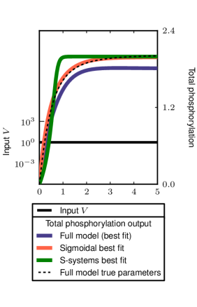
In this multi-site phosphorylation example, the sigmoidal model class is a better performer than the S-systems class. A typical example of performance is depicted in FIG. S4. Though the S-systems class makes predictions that are still qualitatively correct, and its predictions steadily improve as $N$ increases, the sigmoidal class comes closer to the true underlying model with an equal amount of data.

The confidence intervals on the dynamics in FIG. 3 correspond to samples from the posterior over parameters given $N=300$ data points. In the notation of section S.2, this posterior $P(\alpha~{}|~{}\mathrm{data})\propto\exp{\left[-\tilde{\chi}^{2}(\alpha)/2\right]}$. To generate samples from this distribution, we use Metropolis Monte Carlo as implemented in SloppyCell (MyeGutSet07; SloppyCell). As a starting point, we use the best-fit parameters from the model selection procedure, and we sample candidate steps in parameter space from a multidimensional Gaussian corresponding to the Hessian at the best-fit parameters. From $10^{4}$ Monte Carlo steps, the first half are removed to avoid bias from the initial condition, and every 50 of the remaining steps are used as 100 approximately independent samples from the parameter posterior. We note that the median behavior over the Bayesian posterior is less extreme than the behavior at the maximum likelihood parameters (not shown), but still has fast-timescale dynamics indicative of overfitting.

S.1.5 Yeast glycolysis model

As an example of inference of more complicated dynamics, we use a model of oscillations in yeast glycolysis, originally studied in terms of temperature compensation (RuoChrWol03) and since used as a test system for automated inference (SchValJen11). The model’s behavior is defined by ODEs describing the dynamics of the concentrations of seven molecular species (the biological meaning of the species is not important here):

$$\frac{dS_{1}}{dt} = J_{0}-\frac{k_{1}S_{1}S_{6}}{1+(S_{6}/K_{1})^{q}}$$

$$\frac{dS_{2}}{dt} = 2\frac{k_{1}S_{1}S_{6}}{1+(S_{6}/K_{1})^{q}}-k_{2}S_{2}(N-S_{5})-k_{6}S_{2}S_{5}$$

$$\frac{dS_{3}}{dt} = k_{2}S_{2}(N-S_{5})-k_{3}S_{3}(A-S_{6})$$

$$\frac{dS_{4}}{dt} = k_{3}S_{3}(A-S_{6})-k_{4}S_{4}S_{5}-\kappa(S_{4}-S_{5})$$ (S14)

$$\frac{dS_{5}}{dt} = k_{2}S_{2}(N-S_{5})-k_{4}S_{4}S_{5}-k_{6}S_{2}S_{5}$$

$$\frac{dS_{6}}{dt} = -2\frac{k_{1}S_{1}S_{6}}{1+(S_{6}/K_{1})^{q}}+2k_{3}S_{3}(A-S_{6})-k_{5}S_{6}$$

$$\frac{dS_{7}}{dt} = \psi\kappa(S_{4}-S_{5})-kS_{5}.$$

Parameter values, listed in Table S3, are set to match with those used in Ref. (SchValJen11) and Table 1 of Ref. (RuoChrWol03), where our $S_{5}=N_{2}$, our $S_{6}=A_{3}$, and our $S_{7}=S_{4}^{ex}$.

$J_{0}$	2.5	mM min-1
$k_{1}$	100.	mM-1 min-1
$k_{2}$	6.	mM-1 min-1
$k_{3}$	16.	mM-1 min-1
$k_{4}$	100.	mM-1 min-1
$k_{5}$	1.28	min-1
$k_{6}$	12.	mM-1 min-1
$k$	1.8	min-1
$\kappa$	13.	min-1
$q$	4
$K_{1}$	0.52	mM
$\psi$	0.1
$N$	1.	mM
$A$	4.	mM

Table S3: Parameters for the yeast glycolysis model defined in Eqns. (S14).

Figure S5: (Left) Network depicting the yeast glycolysis model defined by Eqns. (S14). Solid arrows represent excitation, solid lines with circles represent inhibition, and dashed arrows represent other types of interaction terms. (Right) Selected sigmoidal network fit to $N=40$ noisy measurements from the yeast glycolysis model, as shown in FIG. 4. Again, arrows represent excitation and circles inhibition, with the thickness of arrows indicating interaction strength. For clarity, self-inhibitory terms for each variable are not shown.

Variable	In-sample IC (mM)	Out-of-sample IC (mM)	In-sample $\sigma$ (mM)
$S_{1}$	[0.15, 1.60]	[0.15, 3.05]	0.04872
$S_{2}$	[0.19, 2.16]	[0.19, 4.13]	0.06263
$S_{3}$	[0.04, 0.20]	[0.04, 0.36]	0.00503
$S_{4}$	0.115	0.115	N/A
$S_{5}$	0.077	0.077	N/A
$S_{6}$	2.475	2.475	N/A
$S_{7}$	0.077	0.077	N/A

Table S4: Initial conditions (IC) and standard deviations of experimental noise ($\sigma$) used in the yeast glycolysis model. Initial conditions for visible species $S_{1}$, $S_{2}$, and $S_{3}$ are chosen uniformly from the given ranges, chosen to match Ref. (SchValJen11). Out-of-sample ranges are each twice as large as in-sample ranges. Initial conditions for the remaining hidden species are fixed at reference initial conditions from Refs. (SchValJen11) and (RuoChrWol03). In-sample noise is set at 10% of the standard deviation of each variable’s concentration in the limit cycle, as quoted in Ref. (SchValJen11).

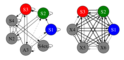
For the yeast glycolysis model, we use as input the initial conditions for the visible species $S_{1}$, $S_{2}$, and $S_{3}$. These are each chosen uniformly from ranges listed in the “In-sample IC” column of Table S4. Each of the three visible species are then measured at a random time uniformly chosen from $0$ to $5$ minutes, meaning the total number of datapoints $N_{D}=3N$ for this system, where $N$ is the number of initial conditions sampled. Gaussian noise is added to each measurement with standard deviations given in Table S4. To evaluate the model’s performance, we test it using 100 new input values selected uniformly from the ranges listed in the “Out-of-sample IC” column of Table S4, each of which is compared to the true model at 100 timepoints evenly spaced from 0 to 5 min. The correlation between the adaptive fit model and the actual model over these 100 timepoints is calculated separately for each visible species, set of initial conditions, and in-sample data, and the average is plotted as the “mean out-of-sample correlation” in FIG. 4. The topology of the selected network model is illustrated in FIG. S5. Note that our model fitting approach assumes that the model timecourse is fully determined (aside from measurement error) by the concentrations of measured species. To be consistent with this assumption we do not vary the initial conditions of the four hidden variables. In future work it may be possible to relax this assumption, allowing the current state of intrinsic variations in hidden variables to be learned as well.

In Ref. (SchValJen11), the EUREQa engine is used to infer the same yeast glycolysis model that we use here. We can roughly compare performance as a function of computational and experimental effort by measuring the number of required model evaluations and measurements (FIG. 4). Here we compare the two approaches in more detail.

First, Ref. (SchValJen11) attempts to match time derivatives of species concentrations as a function of species concentrations, instead of species concentrations as a function of time as we do. This means that each model evaluation is more computationally costly for us, since it requires an integration of the ODEs over time. It also means, however, that we are able to match well the phases of oscillations, which remain unconstrained in Ref. (SchValJen11). The fitting of timecourses instead of derivatives also makes our method focus on the fitting of dynamics near the attractor, rather than attempting to constrain dynamics through the entire phase space.

To consistently infer exact equations for the full 7-dimensional model, Ref. (SchValJen11) used $20,000$ datapoints and roughly $10^{11}$ model evaluations. We contrast this with our method that produces reasonable inferred models using $40$ datapoints and less than $5\times 10^{8}$ model evaluations (FIG. 4).

Finally, in the main text we test the performance of our yeast glycolysis models for out-of-sample ranges of initial conditions that are twice as large as the in-sample ranges from which data is taken, as in Ref. (SchValJen11), in order to more directly test their ability to extrapolate to regimes that were not tested in training. In FIG. S6, we compare this to performance when out-of-sample initial conditions are chosen from the same ranges as in-sample data (note that, nonetheless, none of the test examples has appeared in the training set). Here we see that the mean correlation can reach 0.9 using $N=40$ measurements.

Figure S6: Performance of inferred models of yeast glycolysis as a function of the number of measurements $N$. Here we compare mean correlations produced for out-of-sample initial conditions chosen from ranges twice as large as in-sample ranges (“wide ranges,” plotted in red) to when out-of-sample conditions are chosen from the same ranges as in-sample ranges (“narrow ranges,” plotted in orange). The mean and standard deviation over 5 realizations of in-sample data are shown by filled symbols and shaded regions.

S.2 Derivation of Bayesian log-likelihood estimate $\mathcal{L}$

The derivation here largely follows Refs. (Bal97; BiaNemTis01), but can be traced to the 1970s (Sch78). For a given model $M$ that depends on parameters $\alpha$, our model selection algorithm requires an estimate of the probability that $M$ is the model that produced a given set of data $\{y_{i}\}$ with corresponding error estimates $\{\sigma_{i}\}$ (measured at a set of timepoints $\{t_{i}\}$), and $i=1,\dots,N$, so that there are $N$ measurements. Since the parameters $\alpha$ are unknown aside from a prior distribution $P(\alpha)$, we must integrate over all possible values:

$$P(M~{}|~{}\mathrm{data}) =P(M~{}|~{}\{y_{i},\sigma_{i},t_{i}\})$$ (S15)

$$=Z^{-1}_{\alpha}\int d^{N_{p}}\alpha~{}P(M~{}|~{}\{y_{i},\sigma_{i},t_{i}\};\alpha)~{}P(\alpha),$$ (S16)

where the normalization constant $Z_{\alpha}=\int d^{N_{p}}\alpha~{}P(\alpha)$ and $N_{p}$ is the number of parameters. In terms of the output given the model, Bayes rule states

$$P\left(M~{}|~{}\{y_{i},\sigma_{i},t_{i}\};\alpha\right)=\frac{P\left(M\right)}{P\left(\{y_{i}\}\right)}P\left(\{y_{i}\}~{}|~{}M(\alpha);\{\sigma_{i},t_{i}\}\right).$$ (S17)

Assuming that the model output has normally distributed measurement errors,

$$P\left(\{y_{i}\}~{}|~{}M(\alpha);\{\sigma_{i},t_{i}\}\right) =\prod_{i=1}^{N}P\left(y_{i}~{}|~{}M(\alpha);\sigma_{i};t_{i}\right)$$ (S18)

$$=\prod_{i=1}^{N}\frac{1}{\sqrt{2\pi\sigma_{i}^{2}}}\exp{\left[-\frac{1}{2}\left(\frac{y_{i}-M(t_{i},\alpha)}{\sigma_{i}}\right)^{2}\right]}$$

$$=Z^{-1}_{\sigma}\exp{\left[-\frac{1}{2}\sum_{i=1}^{N}\left(\frac{y_{i}-M(t_{i},\alpha)}{\sigma_{i}}\right)^{2}\right]}$$

$$=Z^{-1}_{\sigma}\exp{\left[-\frac{1}{2}\chi^{2}(M(\alpha),\{y_{i},\sigma_{i},t_{i}\})\right]},$$

where $\chi^{2}$ is the usual goodness-of-fit measure consisting of the sum of squared residuals, and $Z_{\sigma}$ is the normalization constant $\prod_{i=1}^{N}\sqrt{2\pi\sigma_{i}^{2}}$. Thus we have:

$$P(M~{}|~{}\mathrm{data})=CZ^{-1}_{\alpha}\int d^{N_{p}}\alpha~{}~{}\exp{\left[-\frac{1}{2}\tilde{\chi}^{2}(\alpha)\right]},$$ (S19)

where $C\equiv 2P(M)/Z_{\sigma}P\left(\{y_{i}\}\right)$ and $\tilde{\chi}^{2}(\alpha)=\chi^{2}(\alpha)-2\log P(\alpha)$. Since we will be comparing models fitting the same data, and we assume all models have the same prior probability $P(M)$, $C$ will be assumed constant in all further comparisons (but see Ref. (WolMac97) for the discussion of this assumption).

If there are enough data to sufficiently constrain the parameters (as is the case for ideal data in the limit $N\rightarrow\infty$), then the integral will be dominated by the parameters near the single set of best-fit parameters $\alpha_{\mathrm{best}}$. To lowest order in $1/N$, we can approximate the integral using a saddle-point approximation (BiaNemTis01):

$$P(M~{}|~{}\mathrm{data}) \approx CZ^{-1}_{\alpha}\exp{\left[-\frac{1}{2}\tilde{\chi}^{2}(\alpha_{\mathrm{best}})\right]}\int d^{N_{p}}\alpha~{}\exp{\left[-(\alpha-\alpha_{\mathrm{best}})\mathcal{H}(\alpha-\alpha_{\mathrm{best}})\right]},$$ (S20)

where $\mathcal{H}$ is the Hessian:

$$\mathcal{H}_{k\ell}=\frac{1}{2}\frac{\partial^{2}\tilde{\chi}^{2}(\alpha)}{\partial\alpha_{k}d\alpha_{\ell}}\bigg{|}_{\alpha_{\mathrm{best}}}.$$ (S21)

If we assume normally distributed priors on parameters with variances $\varsigma^{2}_{k}$, the log posterior probability becomes

$$\log P(M~{}|~{}\mathrm{data})\approx\mathrm{const}-\frac{1}{2}\tilde{\chi}^{2}(\alpha_{\mathrm{best}})-\frac{1}{2}\sum_{\mu=1}^{N_{p}}\log\lambda_{\mu}-\frac{1}{2}\sum_{k=1}^{N_{p}}\log\varsigma^{2}_{k},$$ (S22)

where $\lambda_{\mu}$ are the eigenvalues of $\mathcal{H}$, and the last term comes from $Z_{\alpha}$. We thus use as our measure of model quality

$$\mathcal{L}\equiv-\frac{1}{2}\tilde{\chi}^{2}(\alpha_{\mathrm{best}})-\frac{1}{2}\sum_{\mu}\log\lambda_{\mu}-\frac{1}{2}\sum_{k}\log\varsigma^{2}_{k}.$$ (S23)

Eq. (S23) is a generalization of the Bayesian Information Criterion (BIC) (Sch78) when parameter sensitivities and priors are explicitly included. The first term is the familiar $\chi^{2}$ “goodness of fit,” and the last two terms constitute the fluctuation “penalty” for overfitting or complexity. Note that here the goodness of fit and the complexity penalty are both functions of the entire dynamics, rather than individual samples, which is not a common application of Bayesian model selection techniques.

S.3 Fitting algorithm

We are given $N$ data points $\mathbf{x}_{i}$ at known times $t_{i}$ and known exogenous parameters $I_{i}$, and with known or estimated variances $\sigma_{i}^{2}$. We are approximating the functions $\vec{F}_{X}$ and $\vec{F}_{Y}$ in Eq. (1), where $\mathbf{y}$ are hidden dynamic model variables, and $\mathbf{x}=\mathbf{x}(t,I)$ and $\mathbf{y}=\mathbf{y}(t,I)$ in general depend on time $t$ and inputs $I$. As described in Section S.2, we fit to the data $\mathbf{x}_{i}$ using a combination of squared residuals from the data and priors $P(\alpha)$ on parameters $\alpha$, which we assume to be Gaussian and centered at zero:

$$\tilde{\chi}^{2}=\sum_{i=1}^{N}\left(\frac{\mathbf{x}_{i}-\mathbf{x}(t_{i},I_{i})}{\sigma_{i}}\right)^{2}+2\sum_{k=1}^{N_{p}}\left(\frac{\alpha_{k}}{\varsigma_{k}}\right)^{2},$$ (S24)

where $F$’s are integrated to produce the model values $\mathbf{x}$ and $\mathbf{y}$:

$$\mathbf{x}(t,I) = \mathbf{x}_{0}(I)+\int_{0}^{t}\vec{F}_{X}(\mathbf{x}(s,I),\mathbf{y}(s,I))~{}ds$$ (S25)

$$\mathbf{y}(t,I) = \mathbf{y}_{0}(I)+\int_{0}^{t}\vec{F}_{Y}(\mathbf{x}(s,I),\mathbf{y}(s,I))~{}ds.$$ (S26)

To fit parameters, we use a two step process akin to simulated annealing that uses samples from a “high temperature” Monte Carlo ensemble as the starting points for local optimization performed using a Levenberg-Marquardt routine. The phenomenological models are implemented using SloppyCell (MyeGutSet07; SloppyCell) in order to make use of its parameter estimation and sampling routines.

Following is a high-level description of the fitting algorithm, with choices of parameters for the examples in the main text listed in Table S5.

1. Choose a model class, consisting of a sequence of nested models indexed by $i$, where the number of parameters $N_{p}$ monotonically increases with $i$. Choose a step size $\Delta p$.

2. Given data at $N_{\mathrm{total}}$ timepoints, fit to data from the first $N$ timepoints, where $N$ is increased to $N_{\mathrm{total}}$ in steps of $\Delta N$.

3. At each $N$, test models of increasing number of parameters $N_{p}$ (stepping by $\Delta p$) until $\mathcal{L}$ consistently decreases (stopping when the last $i_{\mathrm{overshoot}}$ models tested have smaller $\mathcal{L}$ than the maximum). For each model, to calculate $\mathcal{L}$:

   1. Generate an ensemble of starting points in parameter space using Metropolis-Hastings Monte Carlo to sample from $P(\alpha)\propto\exp(-\tilde{\chi}^{2}(\alpha)/2TN_{D})$ with $\tilde{\chi}^{2}$ from (S24). The temperature $T$ is set large to encourage exploration of large regions of parameter space, but if set too large can result in a small acceptance ratio. Infinities and other integration errors are treated as $\tilde{\chi}^{2}=\infty$.

      1. Use as a starting point the best-fit parameters from a smaller $N_{p}$ if a smaller model has been previously fit, or else default parameters.

      2. As a proposal distribution for candidate steps in parameter space, use an isotropic Gaussian with standard deviation $\sqrt{TN_{D}}/\lambda_{\mathrm{max}}$, where $N_{D}$ is the total number of data residuals and $\lambda_{\mathrm{max}}$ is the largest singular value of the Hessian [Eq. (S21)] at the starting parameters.

      3. If this model has previously been fit to less data, use those parameters as an additional member of the ensemble.

   2. Starting from each member of the ensemble, perform a local parameter fit, using Levenberg-Marquardt to minimize $\tilde{\chi}^{2}$ from (S24). Stop when convergence is detected (when the L1 norm of the gradient per parameter is less than avegtol) or when the number of minimization steps reaches maxiter. The best-fit parameters $\alpha^{*}$ are taken from the member of the ensemble with the smallest resulting fitted $\tilde{\chi}^{2}$.

   3. At $\alpha^{*}$, calculate $\mathcal{L}$ from (S23).

4. For each $N$, the model with largest log-likelihood $\mathcal{L}$ is selected as the best-fit model.

$\Delta p$ (gravitation and phosphorylation examples)	$2$
$\Delta p$ (yeast example)	$5$
$i_{\mathrm{overshoot}}$	$3$
Ensemble temperature $T$ (full phosphorylation model)	$10$
Ensemble temperature $T$ (all other models)	$10^{3}$
Total number of Monte Carlo steps (full phosphorylation model)	$10^{2}$
Total number of Monte Carlo steps (all other models)	$10^{4}$
Number of ensemble members used	$10$
avegtol	$10^{-2}$
maxiter	$10^{2}$

Table S5: Adaptive inference algorithm parameters. ¹In the full phosphorylation model, we fit parameters in log-space since they are known to be positive. This makes the model more sensitive to large changes in parameters, meaning that we are forced to be more conservative with taking large steps in parameter space to achieve reasonable acceptance ratios.

S.4 Scaling of computational effort

Figure S7: The number of model evaluations (integrations) used at each $N$, for the multi-site phosphorylation and yeast glycolysis examples. Once the size of model has saturated, we expect the number of evaluations to scale linearly with $N$ (black lines). If the selected model size is growing with $N$, as in the yeast glycolysis example below $N=20$ (see FIG. S8), we expect faster than linear growth.

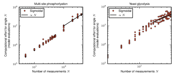
In FIG. S7, we plot the number of model evaluations used in each search for the best-fit phenomenological model. We define a model evaluation as a single integration of a system of ODEs. This includes both integration of model ODEs and the derivatives of model ODEs, used in gradient calculations. Note that in FIG. 4, to indicate the total number of evaluations used as $N$ is gradually increased to its final value, we plot the cumulative sum of the number of model evaluations depicted in FIG. S7. We see that the number of model evaluations scales superlinearly with $N$ if the selected model size is growing with $N$, as is the case in the yeast glycolysis model below about $N=20$ (FIG. S8). When the model size saturates, the number of model evaluations scales roughly linearly with $N$.

Figure S8: Fitting sigmoidal models to the yeast glycolysis oscillation data, the number of total parameters in the selected model, plotted in red, saturates to roughly 65. The solid line compares the number of parameters in the selected model to the number of data points $N_{D}$ used to infer the model. In orange, we plot the effective number of parameters, which we define as the number of directions in parameter space that are constrained by the data such that the corresponding Hessian eigenvalue $\lambda>1$ (compared to parameter priors with eigenvalue $10^{-2}$). We expect the optimal effective number of parameters to stay below $N_{D}$. Shown are the median and full range of values over 5 data realizations.