Testing X-ray Measurements of Galaxy Cluster Outskirts
with
Cosmological Simulations
Abstract
The study of galaxy cluster outskirts has emerged as one of the new frontiers in extragalactic astrophysics and cosmology with the advent of new observations in X-ray and microwave. However, the thermodynamic properties and chemical enrichment of this diffuse and azimuthally asymmetric component of the intra-cluster medium are still not well understood. This work, for the first time, systematically explores potential observational biases in these regions. To assess X-ray measurements of galaxy cluster properties at large radii (), we use mock Chandra analyses of cosmological galaxy cluster simulations. The pipeline is identical to that used for Chandra observations, but the biases discussed in this paper are relevant for all X-ray observations outside of . We find the following from our analysis: (1) filament regions can contribute as much as at to the emission measure, (2) X-ray temperatures and metal abundances from model fitted mock X-ray spectra in a multi-temperature ICM respectively vary to the level of and , (3) resulting density profiles vary to within out to , and gas mass, total mass, and baryon fractions vary all to within a few percent, (4) the bias from a metal abundance extrapolated a factor of 5 higher than the true metal abundance results in total mass measurements biased high by and total gas measurements biased low by and (5) differences in projection and dynamical state of a cluster can lead to gas density slope measurements that differ by a factor of and , respectively. The presented results can partially account for some of the recent gas profile measurements in cluster outskirts by e.g., Suzaku. Our findings are pertinent to future X-ray cosmological constraints with cluster outskirts, which are least affected by non-gravitational gas physics, as well as to measurements probing gas properties in filamentary structures.
Subject headings:
cosmology: theory — clusters: general — galaxies — methods : numerical — X-rays:galaxies:clusters1. Introduction
Clusters of galaxies are the largest gravitationally bound objects in our universe. These objects are massive enough to probe the tension between dark matter and dark energy in structure formation, making them powerful cosmological tools. Cluster-based cosmological tests use observed cluster number counts, the precision of which depends on how well observable-mass relations can constrain cluster masses. Finely tuned observable-mass relations require an understanding of the thermal and chemical structure of galaxy clusters out to large radii, as well as an understanding of systematic biases that may enter into observational measurements of the intracluster medium (ICM).
A new area of study lies in studying the ICM in the outskirts of clusters, a region where the understanding of ICM physics remains incomplete (e.g., see Reiprich et al., 2013, for an overview). Cluster outskirts can be considered to be a cosmic melting pot, where infalling substructure is undergoing virialization and the associated infalling gas clumps are being stripped due to ram pressure, depositing metal-rich gas in the cluster atmosphere, changing thermal and chemical structure of the ICM. Measurements at these regions will allow us to form a more complete assessment of the astrophysical processes, e.g. gas stripping and quenching of star formation in infalling galaxies, that govern the formation and evolution of galaxy clusters and their galaxies.
Gas properties in cluster outskirts are also more suitable for cosmological measurements; the effects of dissipative non-gravitational gas physics, such as radiative cooling and feedback, are minimal in the outskirts compared with the inner regions. Gas density measurements in cluster outskirts will also help constrain the baryon budget. While recent X-ray cluster surveys have provided an independent confirmation of cosmic acceleration and tightened constraints on the nature of dark energy (Allen et al., 2008; Vikhlinin et al., 2009), the best X-ray data, circa 2009, were limited to radii within half of the virial radius, and cluster outskirts were largely unobserved.
Recent measurements from the Suzaku X-ray satellite have pioneered the study of the X-ray emitting ICM in cluster outskirts beyond 111 is the radius of the cluster enclosing an average matter density 200 times the critical density of the Universe. (e.g., Bautz et al., 2009; Reiprich et al., 2009; Hoshino et al., 2010; Kawaharada et al., 2010). These measurements had unexpected results in both entropy and enclosed gas mass fraction at large radii. Entropy profiles from Suzaku data were significantly flatter than theoretical predictions from hydrodynamical simulations (George et al., 2009; Walker et al., 2012), and the enclosed gas mass fraction from gas mass measurements of the Perseus cluster exceeded the cosmic baryon fraction (Simionescu et al., 2011). These results suggest that gasesous inhomogeneities might cause an overestimate in gas density at large radii. Suzaku observations and subsequent studies demonstrated that measurements of the ICM in cluster outskirts are complicated by contributions from the cosmic X-ray background, excess emission from gasesous substructures (Nagai & Lau, 2011; Zhuravleva et al., 2013; Vazza et al., 2013; Roncarelli et al., 2013), and poorly understood ICM physics in the outskirts. However, analyses of cluster outskirts with both Planck Sunyaev-Zel’dovich and ROSAT X-ray measurements found otherwise (Eckert et al., 2013a, b). The mysteries surrounding these X-ray measurements of cluster outskirts are still unsettled due to a number of observational systematic uncertainties, such as X-ray background subtraction.
The latest deep Chandra observations of the outskirts of galaxy cluster Abell 133, a visually relaxed cluster with X-ray temperature keV, have given us an unprecedented opportunity to probe the ICM structure in cluster outskirts (Vikhlinin et al., in prep.). First, the high sub-arcsec angular resolution allows for efficient point source removal, the isolation of the cosmic X-ray background, and the detection of small-scale clumps, which dominate the X-ray flux at large radii. Second, the long exposure time of 2.4 Msec also enables direct observations of the filamentary distribution of gas out to .
To address potential biases that could affect observed ICM properties at large radii, we use mock Chandra observations from high-resolution cosmological simulations of galaxy clusters. The goal of this paper is to characterize the properties of diffuse components of the X-ray emitting ICM in the outskirts of galaxy clusters, and to assess the implications for X-ray measurements. Our analysis focuses on the effects that come from a combination of limited spectral resolution and low photon counts in cluster outskirts, where spectral contributions from metal line emissions become more significant than those from thermal bremsstrahlung emissions.
Our approach is similar in spirit as in Rasia et al. (2008) which pioneered the study of systematics on abundance measurements on the ICM by analyzing the spectral properties of mock plasma spectra generated with XSPEC. We extend the study of XSPEC generated mock spectra to the outskirt regions. Our results are valid for all observations of spectra from plasma with a multicomponent temperature.
Specifically, we look at the accuracy of metal abundance measurements from spectral fitting and their consequential effects on the measurements of projected X-ray temperature, emission measure, deprojected temperature, gas density, gas mass, and hydrostatic mass derived from these profiles. We explore potential biases by (1) measuring contributions of clumps and filaments to emission measurements, (2) testing the modeling of bremsstrahlung and metal line emissions in low density regions, and (3) checking for line of sight dependence in the density slope in cluster outskirts and differences in observed ICM profiles for an unrelaxed cluster.
This work will be useful in assessing the robustness of X-ray measurements beyond , as we test both the spectral fitting of X-ray photons in low density regions, and the validity of fitting formulae that are used to reconstruct ICM profiles.
2. Methodology
2.1. Cosmological simulations
We use a sample of high-resolution cosmological simulations of cluster-sized systems from Nagai et al. (2007a, b, hereafter N07) that assumes a flat CDM universe with , , , and . The Hubble constant is defined as km s-1 Mpc-1, and is the mass variance within spheres of radius Mpc. We simulate these clusters with the Adaptive Refinement Tree (ART) -body+gas-dynamics code (Kravtsov, 1999; Kravtsov et al., 2002; Rudd et al., 2008), an Eulerian code with spatial and temporal adaptive refinement, and non-adaptive mass refinement (Klypin et al., 2001).
Our simulations include radiative cooling, star formation, metal enrichment, stellar feedback, and energy feedback from supermassive black holes (see Avestruz et al., in prep. for more details). Briefly, we seed black hole particles with a seed mass of in dark matter halos with , and allow the black holes to accrete gas according to a modified Bondi accretion model with a density dependent boost factor (Booth & Schaye, 2009). Black holes feed back a fraction of the accreted rest mass energy in the form of thermal energy,
| (1) |
where is the radiative efficiency for a Schwarzschild black hole undergoing radiatively efficient Shakura & Sunyaev accretion (Shakura & Sunyaev, 1973), and is the feedback efficiency parameter tuned to regulate the black hole mass.
We focus on two X-ray luminous clusters from the N07 sample to study the effects of metallicity, line of sight, and dynamical state on X-ray measurements in cluster outskirts. The core-excised X-ray temperatures of CL6 and CL7 are and , respectively. The cluster mass and radii are and for CL6, and and for CL7. Each cluster is selected from simulation box with size Mpc, run on a uniform grid with 8 levels of refinement, and has peak spatial resolution of kpc. The corresponding dark matter particle mass in our regions of interest is . CL6 is an unrelaxed cluster that experienced a 1:1 major merger at , and CL7 is a typical relaxed cluster which has not undergone a major merger for . We refer the reader to N07 for further details.
2.2. Mock Chandra Pipeline
Using our simulated cluster sample, we create realistic mock X-ray maps of simulated clusters by (1) generating an X-ray flux map, and (2) convolving the flux map with the Chandra response files to create photon maps. Below we outline our mock Chandra pipeline, where details can be found in Nagai et al. (2007b).
2.2.1 X-ray Flux maps
We generate X-ray flux maps for each of the simulated clusters along three orthogonal line-of-sight projections. To calculate the flux map, we project X-ray emission from hydrodynamical cells along each line of sight within ( for the clusters in this work) of the cluster center. The X-ray emission as a function of energy from a single hydrodynamical cell of volume is given as,
| (2) |
where , , , and are respectively the electron number density, proton number density, temperature, and metallicity in that cell volume. We compute the X-ray emissivity, , using the MEKAL plasma code (Mewe et al., 1985; Kaastra & Jansen, 1993; Liedahl et al., 1995) and the solar abundance table from Anders & Grevesse (1989). We multiply the plasma spectrum by the photoelectric absorption corresponding to a hydrogen column density of cm-2.
We include results from four different flux maps: (1) , (2) , (3) , and (4) . We generate the flux map from X-ray spectra using all hydrodynamic values directly output from our simulation runs. To isolate the effects of metallicity on our simulated spectra, we use for all -th cell elements in our flux maps and a constant for all -th cell elements in our flux maps. Current observations do not yet probe metal abundance profiles in cluster outskirts, and often extrapolate the abundance at radii beyond . Given the typical range of metallicity that observers have found near () (e.g., Matsushita et al., 2007; Leccardi & Molendi, 2008; Komiyama et al., 2009; Werner et al., 2013), we choose these two values for to bracket a potential range of metallicities in the outskirts. The order of magnitude difference probes how X-ray measurements of the ICM and inferred quantities might be affected by an incorrect extrapolation or mis-measurement of both a metal rich and metal poor environment.
We remove the effects of a multi-temperature medium by fixing both the metal abundance to , and the temperature to keV in the map, which is a characteristic temperature in the outskirts of a galaxy cluster in our probed mass range.
2.2.2 Mock Chandra Photon Maps and Spectra
To simulate mock Chandra data, we convolve the emission spectrum with the response of the Chandra front-illuminated CCDs ACIS (both the Chandra auxiliary response file (ARF) and redistribution matrix file (RMF)) and draw a number of photons at each position and spectral channel from the corresponding Poisson distribution. The photon maps for our mock Chandra data has an exposure time of Msec, comparable to the Msec deep Chandra observations of Abell 133. Since we are interested in probing physical causes for biased X-ray measurements, we do not include any simulated backgrounds.
From our mock photon maps, we generate images in the keV band, and use them to identify and mask out clumps from our analysis. We use the wavelet decomposition algorithm described in Vikhlinin et al. (1998). This procedure is consistent with the small-scale clump removal performed by observers.
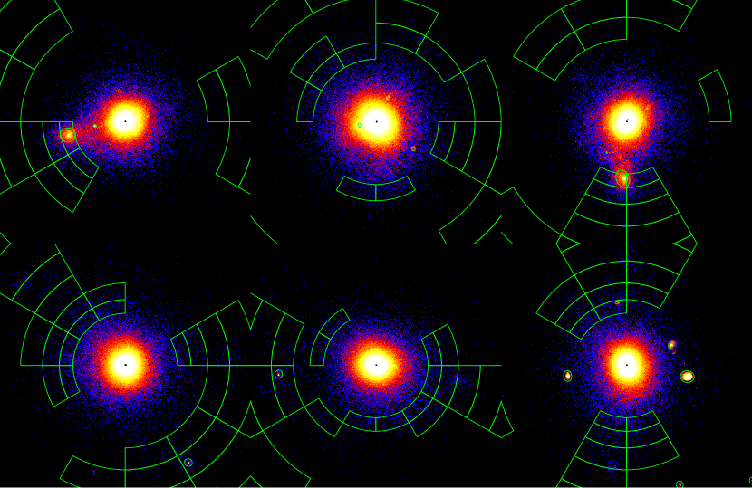
Detected clumps are within a limited flux of erg s-1 cm-2 in the keV energy band, corresponding to a luminosity of erg s-1 for clusters at , the observational redshift of our clusters. Any remaining small-scale structures fall below our clump detection limit. The total gas mass in excluded clumps is no more than a few percent of the total enclosed gas mass.
X-ray emission in cluster outskirts also receive azimuthally asymmetric contributions from filamentary structures. Similar to the analysis of X-ray emission in A133 outskirts, after clump removal, we identify filamentary regions as annular sections with an average flux that exceeds the average flux within the entire annulus. We exclude the filamentary contribution from our final analysis. We include a sample image map with identified clumps and filaments in Figure 1.
From the mock Chandra photon map, we extract a grouped spectrum from concentric annular bins centered on the main X-ray peak. Annular regions are defined with , where and are the outer and inner edges of the annular bin, respectively. The spectra exclude photons from regions corresponding to clumps and filaments. For each spectrum, we perform a single-temperature fit in the keV band using XSPEC version 12.8 with the MEKAL model plasma code and a C-statistic fit (Cash, 1979) to extract the projected X-ray temperature and abundance . We use the same Chandra ARF and RMF files to fit a model spectrum to the mock photon spectra. Temperature, metal abundance, and spectral normalization are the only free parameters in the fit.
2.2.3 Analysis of the ICM
To compare with observed Chandra data, we reconstruct the emission measure profile and repeat the deprojection analysis by Vikhlinin et al. (2006). This analysis reconstructs the spherically averaged density and temperature profiles of the intracluster medium with 3D analytic models. We also estimate the total cluster mass assuming hydrostatic equilibrium from the reconstructed 3D density and temperature profiles.
To calculate the projected emission measure profile , we use two main input ingredients: (1) the azimuthally averaged X-ray surface brightness profile , and (2) the projected 2D X-ray temperature and metallicity profiles described in Section 2.2.2. We can relate the deprojected to the two ingredients as follows,
| (3) |
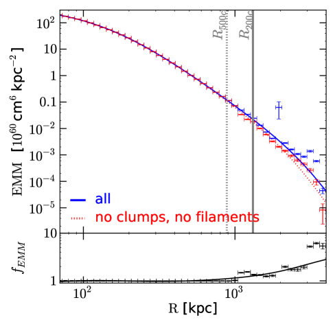
We show the emission measure profile for CL7 along the y-axis, where filamentary features are most prominent in Figure 2, and the corresponding effect of clump and filament removal from the analysis. The solid blue line corresponds to the emission measure profile that include clumps and filamentary substructure, and dotted line corresponds to the emission measure profile that excludes the substructure. The bottom panel shows the ratio between the profile with substructure to the profile without, and illustrates the extent of the excess emission in cluster outskirts. For this cluster, the excess of the best-fit profile can be as much as a factor of 2 at to a factor of 3 at . The errorbars correspond to the binned data, and the excess in individual bins are as high as a factor of 6 in the filamentary regions. Excess emission measure from a substructure is visible at kpc.
We extract the X-ray surface brightness profiles from photons in the keV band in concentric annuli of , giving us a count rate in each annular bin. We use the projected X-ray temperature and metallicity to calculate the MEKAL model plasma emissivity, . With the relation given by Equation (3), we use interpolated values of the model plasma emissivity to convert the count rate into a projected emission measure.
The deprojection process is fully described in Vikhlinin et al. (2006), and can be summarized as follows. The analytic form of our 3D gas density model is given by,
| (4) |
This is a modification of the -model that allows for separate fitting of the gas density slope at small, intermediate, and large radii.
The analytic form of our 3D temperature profile is a product of two terms that describe key features of in observed projected temperature profiles (Vikhlinin et al., 2005),
| (5) |
The first term takes into account the temperature decline at large radii with a broken power law with transition radius, ,
| (6) |
with and as free parameters. The second term models the temperature decline in the central region due to radiative cooling,
| (7) |
We project the 3D model of the temperature profile, weighting multiple temperature components using the algorithm from Vikhlinin et al. (2006). We then fit the projected model to the projected X-ray temperature from our mock data, fitting in the radial range between .
The 3D models for gas density and temperature profiles allow us to estimate the total mass of the cluster, assuming hydrostatic equilibrium,
| (8) |
where is mean molecular weight for the fully ionized ICM, is the proton mass, and we have set the Boltzmann constant to be unity such that the temperature is in unit of energy.
3. Results
To test the MEKAL modeling of bremsstrahlung and metal line emissions in low density regions, we perform the XSPEC fit with a fixed metal abundance parameter: for the map, and for the map. The metallicity in the map is close to the simulation metallicity in cluster outskirts, but we use the map to also check the effects of a possible scenario where a higher abundance of metals sits in cluster outskirts. We then compare results from each case with the case, where we perform the fit for all three parameters.
To eliminate the effects of a multi-temperature medium, we also perform the XSPEC fit on our map. We generate ICM profiles using a the best-fit metal abundance parameter and fixed temperature, and compare with the profiles resulting from the known input metal abundance and temperature value.
3.1. Recovered temperature and density profiles with known abundance measurements
In this section, we check for consistency in gas density measurements from spectral fitting with the XSPEC fit performed using only two free parameters: projected X-ray temperature and normalization of fit. We use the and photon maps for this experiment, and fix the abundance parameter to the true abundance of the map.
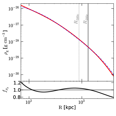
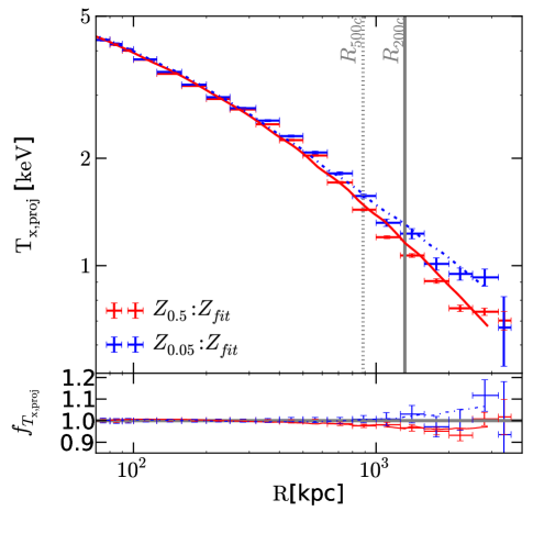
Figure 3 shows the best-fit value for the projected X-ray temperature for each map. In cluster outskirts, the best fit X-ray temperature for the maps is systematically higher than that of the map, and the gas density differs by . Note that while the true temperature of the two maps in each radial bin is identical, their measurements differ up to . The discrepancy points to the degeneracies between fitting parameters. While the fitting procedure assumes a single-temperature fit, the true ICM is a multi-temperature medium, thus requires more degrees of freedom to capture the inhomogeneities. Both the metal abundance and the normalization of the fit offer additional degrees of freedom to minimize the residuals, so it is not surprising that statistically significant differences can arise in measured X-ray temperatures if the metal line contributions are different. We plot the spectra of photons from the radial bin with the largest deviation in measured X-ray temperature in Figure 4. Compared to the spectrum from the photon map (red points), the spectrum from the map (blue points) has a much lower emission from metal line cooling, and therefore it has a suppressed peak in the energy spectrum. The solid lines show the best fit model spectrum for each map.
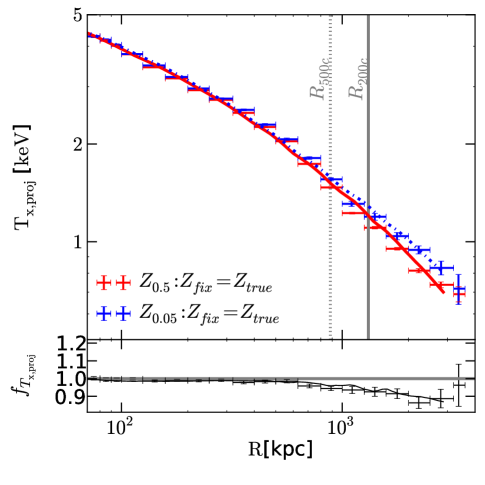
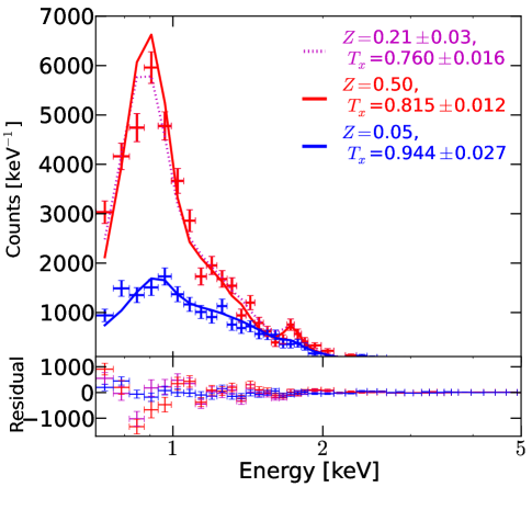
With a metal abundance parameter fixed to the true value of , the model spectrum overshoots the peak of the mock photon spectrum at the Fe-L complex between 0.8 and 1.4 keV, and the best fit X-ray temperature is keV. If we allow the metal abundance to vary as an additional free parameter, both the best fit metal abundance () and the X-ray temperature (keV) are lower and the residual difference between the mock photon counts and the model spectrum improves.
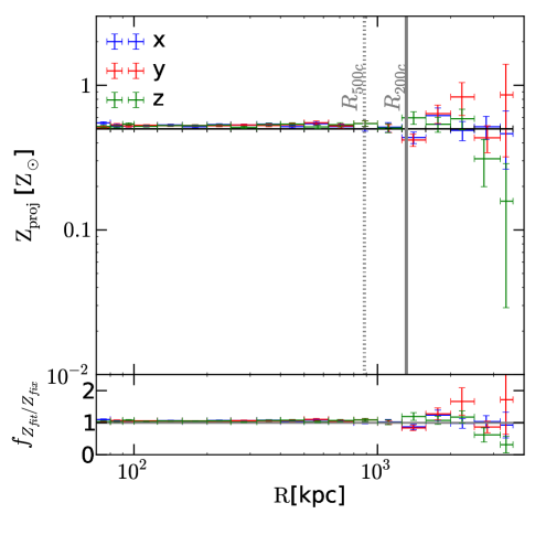
In Figure 5, we show how the systematic bias in metal abundance goes away in the absence of a multi-temperature ICM. The axes show the best fit metal abundance as a function of radius along three different lines of sight for our map. This test isolates biases due to density inhomogeneities, lower photon counts, and instrumental response. For a map with uniform temperature, the fitting procedure well recovers the input constant metallicity, and does not exhibit a systematic decline. The best fit projected X-ray temperature is also well recovered to the fixed input value.
The suppressed peak in the mock photon spectrum in Figure 4 can be attributed to a high temperature phase of gas in the outskirts. For gas with an average temperature of keV, the Fe-L line would be sensitive to a higher temperature component of gas, even if the metallicity of that component is the same (e.g., see Figure 3 in Mazzotta et al. (2004) and Figure 23 in Böhringer & Werner (2010)).
Note, if the abundance parameter were not fixed (magenta dotted line in Figure 4, the best fit abundance parameter would have to be lower than the true value to better minimize the residuals in the fitting procedure. If we were to increase the X-ray temperature in the model spectrum, the residual at the peak would improve, but at the expense of increasing the residual values at other energies.
On the other hand, for the spectra in Figure 4, there are fewer photons from metal line cooling. Hence, most of the spectral features are hidden in Poisson noise. Because of the suppressed spectral features, the fitting procedure produces a best-fit X-ray temperature and normalization that will better minimize the residuals near the peak of the spectrum as opposed to at energies with much fewer counts. To minimize the residuals near the peak, the fitted X-ray temperature must then be higher to harden the model spectrum, which is why the best fit projected X-ray temperature for the map is systematically higher in the outskirts, where photon counts are low.
3.2. Testing metal abundance measurements in cluster outskirts
The robustness of metal abundance measurements in the low density outskirts is not well understood. In this section, we compare the abundance measurements from spectral fitting to the true abundance from our photon maps. We also discuss the effects on the projected X-ray temperature, projected emission measure and the reconstructed three dimensional gas density profile. We begin by comparing variations in projected X-ray temperature and abundance measurements from our and photon maps, where we have set the input metal abundance to constant values.
![[Uncaptioned image]](/html/1404.4634/assets/x7.png)
![[Uncaptioned image]](/html/1404.4634/assets/x9.png)
![[Uncaptioned image]](/html/1404.4634/assets/x10.png)
Figure 6 compares ICM profiles from our and mock X-ray flux maps of CL7, projected along the -axis. Results along other axis projections are qualitatively similar. The top left panel shows the metal abundance measurements retrieved from our mock spectra, fitting the mock spectra to MEKAL model spectra using XSPEC. We define as the ratio between the best fit abundance parameter to the true abundance of our photon map. The profile shows that the while XSPEC fitting procedure recovers a value that is within a factor of 2 of the true input abundance of the photon map, the abundance recovery is significantly worse at larger radii.
For the map, the abundance measurements has a systematic decline from the true value at large radii . As discussed in Section 3.1, the metal abundance parameter adjusts to compensate for the multi-temperature medium when we perform a single-temperture spectral fit. Thus, the best fit abundance parameter will be smaller than the true abundance in order to minimize the residual around the suppressed emission lines. However, if there are too few photons from metal line cooling, the poisson errors become large, and therefore this systematic effect is less apparent since the statistical errors dominate. This is why the last two radial bins do not show underestimation in abundance measurements.
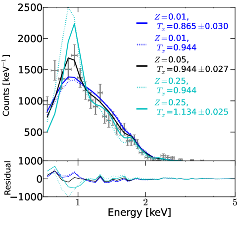
For the map, the photon counts around the peak of the spectrum ( keV) is a factor of three lower than that of the spectrum (See Figure 4). In addition to the intrinsically less pronounced metal lines, the low photon count makes it more difficult for the fitting routine to discern between contributions from metal line cooling and thermal bremsstrahlung emissions, leading to more scatter in the abundance measurements shown in Figure 6. Note that similar scatter is seen in the last two radial bins from the map, which also has a very low photon count.
The top right panel of Figure 6 shows the projected X-ray temperature profile (red and blue points for the respective abundances) from spectral fitting, and the corresponding best fit projected 3D temperature model (thin lines of the same color). We measure the relative bias in as the ratio of the projected X-ray temperature measured with abundance as a free parameter (the profile in Figure 6 compared with the X-ray temperature measured with the abundance parameter fixed to the true abundance of the map (see Figure 3). The X-ray temperature measurements from fits with abundance as a free parameter () vary up to of the measurements with a fixed abundance parameter (). Note, the relative bias in projected X-ray temperature from spectral fitting is in the same direction as that of the abundance measurement.
The cause of the correlation in the relative bias of both the abundance and X-ray temperature becomes evident when we compare model spectra (see Figure 7). When the best fit abundance is higher (lower) than the true abundance, the peak of the model spectrum will sit above (below) the mock spectrum, and a higher (lower) X-ray temperature is necessary to harden (soften) the spectrum to minimize the residuals. Note, while fixing the metal abundance parameter to a value that is five times the true value significantly biases the value of the best fit X-ray temperature parameter, it does not significantly increase the error in the X-ray temperature parameter. The X-ray temperature fit is mostly sensitive to shape of the continuum, and most of the residual contributions to the error in X-ray temperature come from energy bins outside of the Fe-L complex. Here, the model spectra are still within the errorbars of the mock data.
An interesting feature to note in the projected X-ray temperature profile is that the projected 3D temperature model fits the data points well only out to . While the best-fit model profile is within the errorbars of the mock data, it does not capture the emerging trend of the decreasing slope of the projected X-ray temperature at larger radii. The departure from the smooth temperature model profile is indicative of the complicated, inhomogeneous temperature structure in cluster outskirts. The smooth temperature model does not have enough degrees of freedom to account for the bumpier features of the data points, indicating that perhaps a modified fitting formula would be appropriate for total mass measurements outside of .
Note, the errorbars at large radii for the metal abundance measurements are not as good as those of the X-ray temperature measurements because the abundance fitting requires an order of magnitude more photons to have the same statistical uncertainty as the X-ray temperature. The metal abundance is only affected by line emission contributions as opposed to the X-ray temperature, which also has contributions from thermal bremsstrahlung.
From Equation (3), we can see that for the same X-ray surface brightness at a given radius, a higher (lower) gas density is necessary to compensate for a lower (higher) X-ray emissivity . The bottom two panels in Figure 6 show the corresponding projected emission measure and gas density for the same photon maps as in the top two panels. The projected emission measure varies to at all radii, and the gas density to a level of .
We note that the apparent enhanced bias in projected emission measure at intermediate radii for the map, shown in red, is due to effects from integrating over the line of sight. The density profile measured with a fixed abundance parameter is steeper at intermediate radii than the density profile measured with the best fit values for the abundance parameter. Hence, along an equal line of sight, there is a relatively lower emission measure in the fixed abundance case than in the best fit abundance case.
In summary, the relative bias in abundance and projected X-ray temperature are correlated, and vary up to and , respectively. Both the resulting projected emission measure and gas density profiles vary to at low and intermediate radii, but deviate as much as and in emission measure and gas density, respectively.
3.3. Systematic effects of metal abundance measurements on gas profile measurements
As described in Section 3.2, a high (low) bias of the abundance and X-ray temperature measurements would lead to a suppressed (enhanced) density measurement in that radial bin.
In this section, we examine the systematic effects on gas profile measurements with a factor of 2 and 5 bias in the abundance fitting at all radii. For this test, we use the map where we take the metallicity to be constant at throughout the simulation. We choose this value since it is closer to the metal abundance at large radii in our self-consistent cluster simulation with metal enrichment and advection. We run XSPEC fitting by fixing the abundance parameter at metallicities a factor of 2 and 5 from the true value from the map: , and we compare the results to those fitted with the true value . To isolate the effects from all other quantities, we only allow the projected X-ray temperature and the spectral normalization to be free parameters in the fitting .
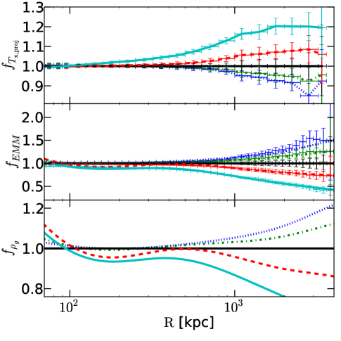
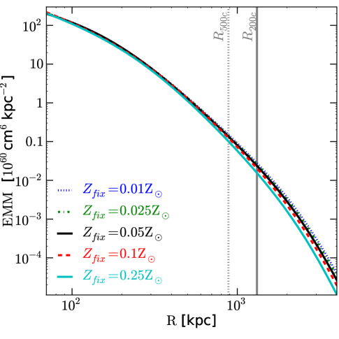
In Figure 8, we plotted the X-ray temperature, projected emission measure, and gas density for each case of and compare to the case (black solid line). Consistent with what we found in Section 3.2, an over (under) estimate of the abundance will lead to suppressed (enhanced) emission measure and subsequently gas density measurements.
If the abundance is measured to within a factor of two of the true metal abundance, the resulting density measurements in the outskirts will be within . However, for the most extreme case of an abundance measurement biased by a factor of 5, the density measurements will have up to a bias.
The emission measure profile on the right panel of Figure 8 shows that an abundance measurement that is higher than the true value can steepen the profile in cluster outskirts. For observational measurements that extrapolate the abundance at large radii, this could introduce an even larger bias in the emission measure, density and temperature. Our tests that fix the abundance measurement to be a factor of two and five times the true abundance show how severely this extrapolation can propagate to inferred quantities, even at . Most notably, for an assumed abundance that is a factor of five higher than the true abundance, the gas density is biased low by .
3.4. Hydrostatic mass and gas mass fraction
From Equation (8), we can see that the X-ray measurement of the hydrostatic mass of the cluster is sensitive to three quantities: the best fit 3D model of the temperature profile, the logarithmic slope of the 3D temperature profile, and the logarithmic slope of the gas density profile. The left panel of Figure 9 illustrates how each of these quantities is affected by a systematic over (under) fit abundance.
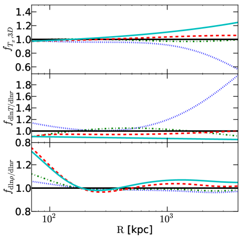
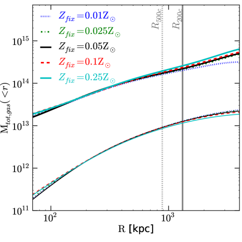
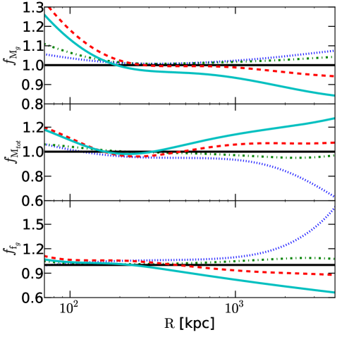
For the case of recovering the metal abundance to within a typical factor of two ( and ), all three quantities are within at intermediate and large radii. At large radii, the bias in the 3D temperature and logarithmic density slope dominate to drive the hydrostatic mass bias in the same direction. A lower temperature fit in the outskirts corresponds to a shallower logarithmic density slope, and therefore a smaller hydrostatic mass (see dotted blue and dot-dashed green thick lines in the right panel of Figure 9). However, the lower fitted temperature and shallower logarithmic slope correspond to a larger enclosed gas mass (see corresponding thin lines in Figure 9), as underestimates in both abundance and temperature lead to overestimates in emission measure, therefore bias the gas density high.
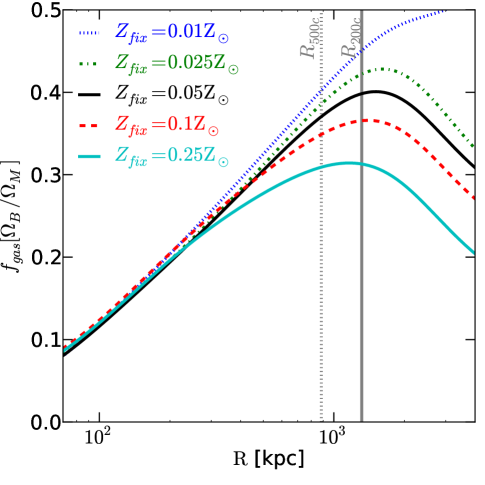
Figure 10 shows that the combined bias in enclosed gas mass and the hydrostatic mass drives the bias in gas fraction up for the low fixed abundance values, and down for the high fixed abundance values. This shows that a poor fit to the X-ray temperature and metallicity in cluster outskirts is potentially causing biases in the Suzaku gas mass fraction measurements at large radii. The same magnitude of errors can come from an incorrectly extrapolated metal abundance in cluster outskirts.
For a standard factor of 2 error in the abundance measurement, the gas mass fraction is only affected by , but any underestimate of the 3D temperature at large radii due to an overly steep poor fit in the deprojection procedure could lead to an even higher gas mass fraction by driving the hydrostatic mass low.
For an abundance that is measured 5 times lower than the true abundance, the measured gas mass fraction could be biased high by given a true abundance of .
While the bias in enclosed gas mass and hydrostatic mass at small radii is rather large, we do not consider this to be representative of biases present in observations; the error in abundance measurement is primarily an issue in the low density outskirts where photon statistics are poor. Additionally, at smaller radii, the gas is much hotter, so the metal abundance and X-ray temperature parameters are less degenerate with each other in the spectral fit.
3.5. Potential issues for gas density slope measurements
We test two potential issues for density slope measurements in cluster outskirts to compare with biases in measurements from spectral fitting and metal abundance extrapolation: projection bias from triaxiality and mass accretion history.
To test the bias due to projection effects from traxiality, we compute the inertia tensors of the gas mass at for our clusters. For CL7, the semi-minor and semi-major axes of the inertia tensor lie almost parallel to the - and -axes respectively, allowing us to use the projections along these axes to make a preliminary assessment of the effects of cluster shape.
To test the effect of accretion history, we compare two clusters, CL6 and CL7 that have similar mass but differ in dynamical states. CL6 has a recent major merger and CL7 has been quiescent since . We compare these two clusters to identify the extent of steepening that is mainly due to recent accretion history.
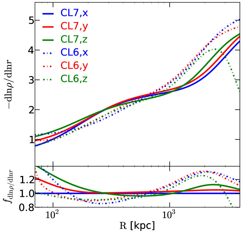
Figure 11 shows the logarithmic gas density slope for our two test cases along various projections, CL6 and CL7. In our relaxed cluster, CL7, the density slope projected along each axis varies by no more than . We would naively expect a significant difference between a line of sight along the semi-major axis (y-axis) and along the semi-minor axis (x-axis). However, the difference in density slope between these two line of sight projections amounts to only a few percent. Effects due to line of sight projection are not likely to significantly steepen observed density profiles.
CL6 is a dynamically disturbed cluster that experienced a 1:1 major merger at , and has a smaller infalling structure at at . The - and -projections correspond to lines of sight that are perpendicular to the plane of accreting substructure. The effects of a merging substructure are visible in the -projection (dotted green), where the density slope is no longer monotonically increasing at larger radii. The outskirts of CL6 cluster along the - and -projections have an observed density profile that exceeds the density slope along the -projection of CL7 by , confirming that X-ray observations should be able to see a difference in density slope between clusters of varying accretion histories.
These two mechanisms have the potential to contribute additional bias to the observed density slope than the bias introduced from spectral fitting ().
4. Summary and Discussion
The study of galaxy cluster outskirts is the new frontier in cluster-based cosmology. In this work, we used cosmological simulations of galaxy clusters to investigate potential biases in metal abundance measurements from X-ray spectra in the low density cluster outskirts (), where metal line cooling contributions become significant. Using X-ray maps with a constant input metal abundance, we showed how systematically biased metal abundance measurements affect ICM quantities such as the gas density and temperature profiles.
In order to test other potential sources of systematic uncertainty in density slope measurements from Chandra observations of Abell 133 (Vikhlinin et al., in prep.), we performed our mock X-ray analysis for projections along the semi-major and semi-minor axes of a relaxed cluster, and for a dynamically disturbed cluster.
To summarize our findings:
-
•
Metal abundance measurements in the outskirts of our test case of a relaxed cluster shows that the metal abundance is best recovered to within a factor of two. Due to the presence of a multi-temperature medium, strong metal line contributions will be systematically biased low. In the regime of few photon counts (either from low X-ray surface brightness or low abundance), accurate metal line contributions will be difficult to recover from Poisson noise.
-
•
An incorrect measurement of the abundance in the low density regions corresponds to fluctuations in measured projected X-ray temperature to within . This temperature bias drives the projected emission measure in a direction opposite of the bias, thus affecting the gas density measurements as much as in the outskirts out to .
-
•
We test the extent of biases that may arise from incorrectly extrapolating the metal abundance measurement in galaxy cluster outskirts by fixing the metal abundance to a factor of 2 and a factor of 5 above and below the true abundance. An abundance assumed a factor of 5 too high biases the gas density measurement and the enclosed total mass by as much as at .
-
•
In the cluster outskirts, an X-ray temperature that is biased low by corresponds to a decrease in the total mass measurement, increase in the enclosed gas mass, and therefore a boosted gas mass fraction by .
-
•
Two potential physical mechanisms for the derived sharpening of density gradients in cluster outskirts are projection and dynamical state of the cluster. Our test cases show that these contribute to no more than and , respectively, to the logarithmic gas density slope. The bias due to an incorrect abundance measurement would affect the density slope by no more than .
We note that fully testing the accuracy of X-ray measurements in cluster outskirts requires a comparison of measurements of ICM properties directly from the simulation with 3D filaments removed in a self-consistent manner with our projected filament finder. While the test cases used in this study do not include high mass clusters, any bias from incorrect abundance measurements would not exceed the bias found in the lower mass counterparts. High mass clusters have larger temperatures at , resulting in a decreased relative contribution of metal line emissions to the X-ray emission measure. This analysis does not include any contributions from simulated backgrounds, and the effects of instrumental and X-ray backgrounds are additional sources of systematic biases that have not been accounted for in our discussions.
Furthermore, our analysis does not take into account non-equilibrium electrons at large radii, which have a lower temperature than the mean ICM gas temperature (Rudd & Nagai, 2009). The temperature bias from non-equilibrium electrons is small in clusters of the mass scales we tested, and we expect non-equilibrium electrons to have less of an effect on the emission measure in the cluster outskirts than biases from metal abundance measurements. Metal line contributions have a significant contribution to the X-ray emission in the low density cluster outskirts, and the X-ray emission has a weak dependence on any biases in the temperature at all radii (). Alternatively, in higher mass clusters, non-equilibrium electrons have larger deviations from the mean ICM gas temperature because the equilibration timescale is longer. The corresponding biases in X-ray measurements of the outskirts of high mass clusters is a topic for future work.
Our findings emphasize the need for long exposure times to have accurate measurements of metal abundance and X-ray temperature in the low density outskirts of galaxy clusters. Accurate X-ray measurements of the hydrostatic mass require an additional term in the temperature modeling in cluster outskirts to account for the shallow slope in the outermost radii. Additionally, accounting for errors in the metal abundance measurement will require more careful modeling of the thermal and chemical structure in cluster outskirts.
In addition to gas inhomogeneities (e.g., Nagai & Lau, 2011), biased measurements of the metal abundance in cluster outskirts may partially explain the enhanced gas mass fraction (e.g., Simionescu et al., 2011) and flattened entropy profiles (e.g., Walker et al., 2012) observed in cluster outskirts. Errors in metal abundance could produce enhanced emission measurements and a steeper 3D temperature profile, leading to overestimates in gas mass and underestimates in hydrostatic mass.
We have identified three potential mechanisms that contribute to density steepening in our mock data, and may affect the observed density slope beyond : (1) overestimation of the abundance, (2) a line of sight corresponding to the semi-minor axis, and (3) rapid recent mass accretion. For (1), the biases introduced by spectral fitting are not likely to exceed . The two physical mechanisms (2) and (3) had respective effects of and .
The mass accretion rate of a galaxy cluster can influence its DM density (Cuesta et al., 2008; Diemer & Kravtsov, 2014) and gas profiles (E.T. Lau et al., in prep.). Accurate measurements of gas density and temperature profiles from X-ray observations of cluster outskirts will provide information on the recent mass accretion history of a galaxy cluster, which is one of the dominant systematics in mass-observable relations in cluster cosmology. Deep observations of cluster outskirts will allow us to better understand the growth of galaxy clusters through mass accretion from the surrounding filamentary structures.
A careful consideration of all potential biases that enter into ICM measurements in galaxy cluster outskirts will enable us to fully use clusters as cosmological probes. Results from this work will also be useful for future missions, such as SMART-X 222 http://smart-x.cfa.harvard.edu/ and Athena+ 333http://athena2.irap.omp.eu/, which will begin mapping the denser parts of the filamentary cosmic web.
References
- Allen et al. (2008) Allen, S. W., Rapetti, D. A., Schmidt, R. W., et al. 2008, MNRAS, 383, 879
- Anders & Grevesse (1989) Anders, E., & Grevesse, N. 1989, Geochim. Cosmochim. Acta, 53, 197
- Bautz et al. (2009) Bautz, M. W., Miller, E. D., Sanders, J. S., et al. 2009, PASJ, 61, 1117
- Böhringer & Werner (2010) Böhringer, H., & Werner, N. 2010, A&A Rev., 18, 127
- Booth & Schaye (2009) Booth, C. M., & Schaye, J. 2009, MNRAS, 398, 53
- Cash (1979) Cash, W. 1979, ApJ, 228, 939
- Cuesta et al. (2008) Cuesta, A. J., Prada, F., Klypin, A., & Moles, M. 2008, MNRAS, 389, 385
- Diemer & Kravtsov (2014) Diemer, B., & Kravtsov, A. V. 2014, ArXiv e-prints, arXiv:1401.1216
- Eckert et al. (2013a) Eckert, D., Ettori, S., Molendi, S., Vazza, F., & Paltani, S. 2013a, A&A, 551, A23
- Eckert et al. (2013b) Eckert, D., Molendi, S., Vazza, F., Ettori, S., & Paltani, S. 2013b, A&A, 551, A22
- George et al. (2009) George, M. R., Fabian, A. C., Sanders, J. S., Young, A. J., & Russell, H. R. 2009, MNRAS, 395, 657
- Hoshino et al. (2010) Hoshino, A., Henry, J. P., Sato, K., et al. 2010, PASJ, 62, 371
- Kaastra & Jansen (1993) Kaastra, J. S., & Jansen, F. A. 1993, A&AS, 97, 873
- Kawaharada et al. (2010) Kawaharada, M., Okabe, N., Umetsu, K., et al. 2010, ApJ, 714, 423
- Klypin et al. (2001) Klypin, A., Kravtsov, A. V., Bullock, J. S., & Primack, J. R. 2001, ApJ, 554, 903
- Komiyama et al. (2009) Komiyama, M., Sato, K., Nagino, R., Ohashi, T., & Matsushita, K. 2009, PASJ, 61, 337
- Kravtsov (1999) Kravtsov, A. V. 1999, PhD thesis, New Mexico State Univ.
- Kravtsov et al. (2002) Kravtsov, A. V., Klypin, A., & Hoffman, Y. 2002, ApJ, 571, 563
- Leccardi & Molendi (2008) Leccardi, A., & Molendi, S. 2008, A&A, 487, 461
- Liedahl et al. (1995) Liedahl, D. A., Osterheld, A. L., & Goldstein, W. H. 1995, ApJ, 438, L115
- Matsushita et al. (2007) Matsushita, K., Fukazawa, Y., Hughes, J. P., et al. 2007, PASJ, 59, 327
- Mazzotta et al. (2004) Mazzotta, P., Rasia, E., Moscardini, L., & Tormen, G. 2004, MNRAS, 354, 10
- Mewe et al. (1985) Mewe, R., Gronenschild, E. H. B. M., & van den Oord, G. H. J. 1985, A&AS, 62, 197
- Nagai et al. (2007a) Nagai, D., Kravtsov, A. V., & Vikhlinin, A. 2007a, ApJ, 668, 1
- Nagai & Lau (2011) Nagai, D., & Lau, E. T. 2011, ApJ, 731, L10
- Nagai et al. (2007b) Nagai, D., Vikhlinin, A., & Kravtsov, A. V. 2007b, ApJ, 655, 98
- Rasia et al. (2008) Rasia, E., Mazzotta, P., Bourdin, H., et al. 2008, ApJ, 674, 728
- Reiprich et al. (2013) Reiprich, T. H., Basu, K., Ettori, S., et al. 2013, Space Sci. Rev., 177, 195
- Reiprich et al. (2009) Reiprich, T. H., Hudson, D. S., Zhang, Y.-Y., et al. 2009, A&A, 501, 899
- Roncarelli et al. (2013) Roncarelli, M., Ettori, S., Borgani, S., et al. 2013, MNRAS, 432, 3030
- Rudd & Nagai (2009) Rudd, D. H., & Nagai, D. 2009, ApJ, 701, L16
- Rudd et al. (2008) Rudd, D. H., Zentner, A. R., & Kravtsov, A. V. 2008, ApJ, 672, 19
- Shakura & Sunyaev (1973) Shakura, N. I., & Sunyaev, R. A. 1973, A&A, 24, 337
- Simionescu et al. (2011) Simionescu, A., Allen, S. W., Mantz, A., et al. 2011, Science, 331, 1576
- Vazza et al. (2013) Vazza, F., Eckert, D., Simionescu, A., Brüggen, M., & Ettori, S. 2013, MNRAS, 429, 799
- Vikhlinin et al. (2006) Vikhlinin, A., Kravtsov, A., Forman, W., et al. 2006, ApJ, 640, 691
- Vikhlinin et al. (2005) Vikhlinin, A., Markevitch, M., Murray, S. S., et al. 2005, ApJ, 628, 655
- Vikhlinin et al. (1998) Vikhlinin, A., McNamara, B. R., Forman, W., et al. 1998, ApJ, 502, 558
- Vikhlinin et al. (2009) Vikhlinin, A., Kravtsov, A. V., Burenin, R. A., et al. 2009, ApJ, 692, 1060
- Walker et al. (2012) Walker, S. A., Fabian, A. C., Sanders, J. S., & George, M. R. 2012, MNRAS, 427, L45
- Werner et al. (2013) Werner, N., Urban, O., Simionescu, A., & Allen, S. W. 2013, Nature, 502, 656
- Zhuravleva et al. (2013) Zhuravleva, I., Churazov, E., Kravtsov, A., et al. 2013, MNRAS, 428, 3274