Control point based exact description of higher dimensional
trigonometric and hyperbolic curves and multivariate surfaces

Abstract

Using the normalized B-bases of vector spaces of trigonometric and hyperbolic polynomials of finite order, we specify control point configurations for the exact description of higher dimensional (rational) curves and (hybrid) multivariate surfaces determined by coordinate functions that are exclusively given either by traditional trigonometric or hyperbolic polynomials in each of their variables. The usefulness and applicability of theoretical results and proposed algorithms are illustrated by many examples that also comprise the control point based exact description of several famous curves (like epi- and hypocycloids, foliums, torus knots, Bernoulli’s lemniscate, hyperbolas), surfaces (such as pure trigonometric or hybrid surfaces of revolution like tori and hyperboloids, respectively) and 3-dimensional volumes. The core of the proposed modeling methods relies on basis transformation matrices with entries that can be efficiently obtained by order elevation. Providing subdivision formulae for curves described by convex combinations of these normalized B-basis functions and control points, we also ensure the possible incorporation of all proposed techniques into today’s CAD systems.

1 Introduction

Normalized B-bases (a comprehensive study of which can be found in Pena1999 and references therein) are normalized totally positive bases that imply optimal shape preserving properties for the representation of curves described as linear combinations of control points and basis functions. Similarly to the classical Bernstein polynomials

$$\mathcal{B}_{n}=\left\{\dbinom{n}{i}u^{i}\left(1-u\right)^{n-i}:u\in\left[0,1\right]\right\}_{i=0}^{n}$$

of degree $n\in\mathbb{N}$ – that in fact form the normalized B-basis of the vector space of polynomials

$$\mathbb{P}_{n}=\left\{1,u,\ldots,u^{n}:u\in\left[0,1\right]\right\}$$

of degree at most $n$ on the compact interval $\left[0,1\right]$, cf. Carnicer1993 – normalized B-bases provide shape preserving properties like closure for the affine transformations of the control polygon, convex hull, variation diminishing (which also implies convexity preserving of plane control polygons), endpoint interpolation, monotonicity preserving, hodograph and length diminishing, and a recursive corner cutting algorithm (also called B-algorithm) that is the analogue of the de Casteljau algorithm of Bézier curves. Among all normalized totally positive bases of a given vector space of functions a normalized B-basis is the least variation diminishing and the shape of the generated curve more mimics its control polygon. Important curve design algorithms like evaluation, subdivision, degree elevation or knot insertion are in fact corner cutting algorithms that can be treated in a unified way by means of B-algorithms induced by B-bases.

These advantageous properties make normalized B-bases ideal blending function system candidates for curve (and surface) modeling. Using B-basis functions, our objective is to provide control point based exact description for higher order derivatives of trigonometric and hyperbolic curves specified with coordinate functions given in traditional parametric form, i.e., in vector spaces

$$\mathbb{T}_{2n}^{\alpha}=\operatorname{span}\mathcal{T}_{2n}^{\alpha}=\operatorname{span}\left\{\cos\left(ku\right),\sin\left(ku\right):u\in\left[0,\alpha\right]\right\}_{k=0}^{n}$$ (1)

or

$$\mathbb{H}_{2n}^{\alpha}=\operatorname{span}\mathcal{H}_{2n}^{\alpha}=\operatorname{span}\left\{\cosh\left(ku\right),\sinh\left(ku\right):u\in\left[0,\alpha\right]\right\}_{k=0}^{n},$$ (2)

where $\alpha$ is a fixed strictly positive shape (or design) parameter which is either strictly less than $\pi$, or it is unbounded from above in the trigonometric and hyperbolic cases, respectively. The obtained results will also be extended for the control point based exact description of the rational counterpart of these curves and of higher dimensional multivariate (rational) surfaces that are also specified by coordinate functions given in traditional trigonometric or hyperbolic form along of each of their variables.

Remark 1.1

From the point of view of control point based exact description of smooth (rational) trigonometric closed curves and surfaces (i.e., when $\alpha=2\pi$), articles RothJuhasz2010  and JuhaszRoth2010 already provided control point configurations by using the so-called cyclic basis functions introduced in RothEtAl2009 . Although this special cyclic basis of $\mathbb{T}_{2n}^{2\pi}$ fulfills some important properties (like positivity, normalization, cyclic variation diminishing, cyclic symmetry, singularity free parametrization, efficient explicit formula for arbitrary order elevation), it is not totally positive, hence it is not a B-basis, since, as it was shown in Pena1997 , the vector space (1) has no normalized totally positive bases when $\alpha\geq\pi$. Therefore, by using the B-basis of (1), the control point based exact description of arcs, patches or volume entities of higher dimensional (rational) trigonometric curves and multivariate surfaces given in traditional parametric form remained, at least for us, an interesting and challenging question.

The rest of the paper is organized as follows. Section 2 briefly recalls some basic properties of rational Bézier curves and points out that curves described as linear combinations of control points and B-basis functions of vector spaces (1) or (2) are in fact special reparametrizations of specific classes of rational Bézier curves. This section also defines control point based (rational) trigonometric and hyperbolic curves of finite order, briefly reviews some of their (geometric) properties like order elevation and asymptotic behavior and at the same time also describes their subdivision algorithm which, to the best of our knowledge, were either totally not detailed or not described with full generality for these type of curves in the literature. Based on multivariate tensor products of trigonometric and hyperbolic curves, Section 3 defines higher dimensional multivariate (rational) trigonometric and hyperbolic surfaces. Section 4 provides efficient and parallely implementable recursive formulae for those base changes that transform the normalized B-bases of vector spaces (1) and (2) to their corresponding canonical (traditional) bases, respectively. Using these transformations, theorems and algorithms of Section 5 provide control point configurations for the exact description of large classes of higher dimensional (rational) trigonometric or hyperbolic curves and multivariate (hybrid) surfaces. All examples included in this section emphasize the applicability and usefulness of the proposed curve and surface modeling tools. Finally, Section 6 closes the paper with our final remarks.

2 Special parametrizations of a class of rational Bézier curves

Using Bernstein polynomials, a rational Bézier curve of even degree $2n$ can be described as

$$\mathbf{r}_{2n}\left(v\right)=\frac{{\displaystyle\sum\limits_{i=0}^{2n}}w_{i}\mathbf{d}_{i}B_{i}^{2n}\left(v\right)}{{\displaystyle\sum\limits_{j=0}^{2n}}w_{j}B_{j}^{2n}\left(v\right)},~{}v\in\left[0,1\right],$$ (3)

where $\left[\mathbf{d}_{i}\right]_{i=0}^{2n}\in\mathcal{M}_{1,2n+1}\left(\mathbb{R}^{\delta}\right)$ is a user defined control polygon ($\delta\geq 2$), while $\left[w_{i}\right]_{i=0}^{2n}\in\mathcal{M}_{1,2n+1}\left(\mathbb{R}_{+}\right)$ is also a user specified non-negative weight vector of rank $1$ (i.e., $\sum_{i=0}^{2n}w_{i}\neq 0$).

For any fixed ratio $v\in\left[0,1\right]$, the recursive relations

$$\left\{\begin{array}[c]{l}w_{i}^{r}\left(v\right)=\left(1-v\right)w_{i}^{r-1}\left(v\right)+vw_{i+1}^{r-1}\left(v\right),\\ \\ \mathbf{d}_{i}^{r}\left(v\right)=\left(1-v\right)\dfrac{w_{i}^{r-1}\left(v\right)}{w_{i}^{r}\left(v\right)}\mathbf{d}_{i}^{r-1}\left(v\right)+v\dfrac{w_{i+1}^{r-1}\left(v\right)}{w_{i}^{r}\left(v\right)}\mathbf{d}_{i+1}^{r-1}\left(v\right),~{}r=1,2,\ldots,2n,~{}i=0,1,\ldots,2n-r\end{array}\right.$$ (4)

with initial conditions

$$w_{i}^{0}\left(v\right)\equiv w_{i},~{}\mathbf{d}_{i}^{0}\left(v\right)\equiv\mathbf{d}_{i},~{}i=0,1,\ldots,2n$$

define the B-algorithm (or rational de Casteljau algorithm) of the curve (3) (cf. Farin2002 ).

We will produce control point exact based description of trigonometric and hyperbolic curves, therefore we need proper bases for vector spaces (1) and (2) of trigonometric and hyperbolic polynomials of order at most $n$ (or of degree at most $2n$), respectively. In what follows, $\overline{\mathcal{T}}_{2n}^{\alpha}$ and $\overline{\mathcal{H}}_{2n}^{\alpha}$ denote the normalized B-bases of vector spaces $\mathbb{T}_{2n}^{\alpha}$ and $\mathbb{H}_{2n}^{\alpha}$, respectively.

2.1 Trigonometric curves and their rational counterpart

Let $\alpha\in\left(0,\pi\right)$ be an arbitrarily fixed parameter and consider the linearly reparametrized version of the B-basis

$$\overline{\mathcal{T}}_{2n}^{\alpha}=\left\{T_{2n,i}^{\alpha}\left(u\right):u\in\left[0,\alpha\right]\right\}_{i=0}^{2n}=\left\{t_{2n,i}^{\alpha}\sin^{2n-i}\left(\frac{\alpha-u}{2}\right)\sin^{i}\left(\frac{u}{2}\right):u\in\left[0,\alpha\right]\right\}_{i=0}^{2n}$$ (5)

of order $n$ (degree $2n$) specified in Sanchez1998 , where the non-negative normalizing coefficients

$$t_{2n,i}^{\alpha}=\frac{1}{\sin^{2n}\left(\frac{\alpha}{2}\right)}\sum_{r=0}^{\left\lfloor\frac{i}{2}\right\rfloor}\binom{n}{i-r}\binom{i-r}{r}\left(2\cos\left(\frac{\alpha}{2}\right)\right)^{i-2r},~{}i=0,1,\ldots,2n$$

fulfill the symmetry property

$$t_{2n,i}^{\alpha}=t_{2n,2n-i}^{\alpha},~{}i=0,1,\ldots,n\text{.}$$ (6)

Definition 2.1 (Trigonometric curves)

A trigonometric curve of order $n$ (degree $2n$) can be described as the convex combination

$$\mathbf{t}_{n}^{\alpha}\left(u\right)=\sum_{i=0}^{2n}\mathbf{d}_{i}T_{2n,i}^{\alpha}\left(u\right),~{}u\in\left[0,\alpha\right],$$ (7)

where $\left[\mathbf{d}_{i}\right]_{i=0}^{2n}\in\mathcal{M}_{1,2n+1}\left(\mathbb{R}^{\delta}\right)$ defines its control polygon.

As stated in Remark 2.2 curves of type (7) can also be obtained as a special trigonometric reparametrization of a class of rational Bézier curves of even degree.

Remark 2.2 (Trigonometric reparametrization)

Using the function

$$\left\{\begin{array}[c]{l}v:\left[0,\alpha\right]\rightarrow\left[0,1\right],\\ \\ v\left(u\right)=\dfrac{1}{2}+\dfrac{\tan\left(\frac{u}{2}-\frac{\alpha}{4}\right)}{2\tan\left(\frac{\alpha}{4}\right)}=\dfrac{\sin\left(\frac{u}{2}\right)}{2\cos\left(\frac{\alpha}{4}-\frac{u}{2}\right)\sin\left(\frac{\alpha}{4}\right)}\end{array}\right.$$ (8)

and weights

$$w_{i}=\frac{t_{2n,i}^{\alpha}}{\binom{2n}{i}},~{}i=0,1,\ldots,2n,$$ (9)

one can reparametrize the rational Bézier curve (3) into the trigonometric form (7). Indeed, one has that

$$w_{i}B_{i}^{2n}\left(v\left(u\right)\right) =\frac{t_{2n,i}^{\alpha}}{\binom{2n}{i}}\binom{2n}{i}v^{i}\left(u\right)\left(1-v\left(u\right)\right)^{2n-i}$$

$$=t_{2n,i}^{\alpha}\cdot\dfrac{\sin^{i}\left(\frac{u}{2}\right)}{2^{i}\cos^{i}\left(\frac{\alpha}{4}-\frac{u}{2}\right)\sin^{i}\left(\frac{\alpha}{4}\right)}\cdot\frac{\sin^{2n-i}\left(\frac{\alpha-u}{2}\right)}{2^{2n-i}\cos^{2n-i}\left(\frac{\alpha}{4}-\frac{u}{2}\right)\sin^{2n-i}\left(\frac{\alpha}{4}\right)}$$

$$=\frac{1}{2^{2n}\cos^{2n}\left(\frac{\alpha}{4}-\frac{u}{2}\right)\sin^{2n}\left(\frac{\alpha}{4}\right)}\cdot T_{2n,i}^{\alpha}\left(u\right)$$

for all $i=0,1,\ldots,2n$ and $u\in\left[0,\alpha\right]$, therefore

$$\mathbf{r}_{2n}\left(v\left(u\right)\right)=\frac{{\displaystyle\sum\limits_{i=0}^{2n}}w_{i}\mathbf{d}_{i}B_{i}^{2n}\left(v\left(u\right)\right)}{{\displaystyle\sum\limits_{j=0}^{2n}}w_{j}B_{j}^{2n}\left(v\left(u\right)\right)}=\frac{{\displaystyle\sum\limits_{i=0}^{2n}}\mathbf{d}_{i}T_{2n,i}^{\alpha}\left(u\right)}{{\displaystyle\sum\limits_{j=0}^{2n}}T_{2n,j}^{\alpha}\left(u\right)}={\displaystyle\sum\limits_{i=0}^{2n}}\mathbf{d}_{i}T_{2n,i}^{\alpha}\left(u\right)=\mathbf{t}_{n}^{\alpha}\left(u\right),~{}\forall u\in\left[0,\alpha\right],$$

since the function system (5) is normalized, i.e., $\sum_{j=0}^{2n}T_{2n,j}^{\alpha}\left(u\right)\equiv 1$, $\forall u\in\left[0,\alpha\right]$. Basis functions (5) and the reparametrization function (8) were repeatedly applied in articles Sanchez1990 , Sanchez1997 and Sanchez1998 , however the (inverse) transformation between bases $\overline{\mathcal{T}}_{2n}^{\alpha}$ and $\mathcal{T}_{2n}^{\alpha}$ were calculated only up to second order in (Sanchez1998, , p. 916) with the aid of a computer algebra system, moreover subdivision of such curves was detailed only for very special control point configurations in Sanchez1990 .

Remark 2.3 (B-algorithm of trigonometric curves)

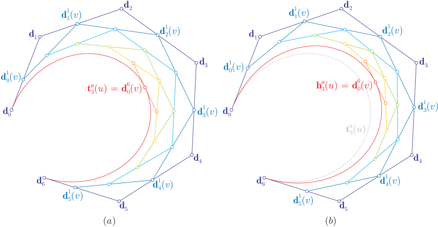
Due to Remark 2.2, the subdivision algorithm of trigonometric curves of type (7) is a simple corollary of the rational de Casteljau algorithm (4). One has to apply the parameter transformation (8) and initial weights (9) in recursive formulae (4). Fig. 1(a) shows the steps of this special variant of the classical rational corner cutting algorithm in case of a third order trigonometric curve.

Figure 1: Consider the fixed control polygon $\left[\mathbf{d}_{i}\right]_{i=0}^{6}$ and the shape parameter $\alpha=\frac{\pi}{2}$ that generate third order trigonometric and hyperbolic curves of the type (7) and (15), respectively. Cases (a) and (b) illustrate the subdivision of these curve at the common parameter value $u=\frac{\pi}{4}$. (The parameter value $\left.v\left(u\right)\right|_{u=\frac{\pi}{4}}=\frac{1}{2}$ is generated by reparametrization functions (8) and (16), respectively.)

The order elevation of trigonometric curves of type (9) was also considered in (Sanchez1998, , Section 4.2). This method will be one of the main auxiliary tools used by the present paper, therefore we briefly recall this process, by using our notations.

Remark 2.4 (Order elevation of trigonometric curves)

Multiplying the curve (7) with the first order constant function

$$1\equiv T_{2,0}^{\alpha}\left(u\right)+T_{2,1}^{\alpha}\left(u\right)+T_{2,2}^{\alpha}\left(u\right),~{}\forall u\in\left[0,\alpha\right]$$

and applying the product rule

$$T_{2n,i}^{\alpha}\left(u\right)T_{2m,j}^{\alpha}\left(u\right)=\frac{t_{2n,i}^{\alpha}t_{2m,j}^{\alpha}}{t_{2\left(n+m\right),i+j}^{\alpha}}T_{2\left(n+m\right),i+j}^{\alpha}\left(u\right),~{}\forall u\in\left[0,\alpha\right],$$

one obtains the trigonometric curve

$$\mathbf{t}_{n+1}^{\alpha}\left(u\right)=\sum_{r=0}^{2\left(n+1\right)}\mathbf{e}_{r}T_{2\left(n+1\right),r}^{\alpha}\left(u\right),~{}u\in\left[0,\alpha\right]$$

of order $n+1$ such that

$$\mathbf{t}_{n+1}^{\alpha}\left(u\right)=\mathbf{t}_{n}^{\alpha}\left(u\right),~{}\forall u\in\left[0,\alpha\right],$$

where

$$\left\{\begin{array}[c]{lcl}\mathbf{e}_{0}&=&\mathbf{d}_{0}\dfrac{t_{2n,0}^{\alpha}t_{2,0}^{\alpha}}{t_{2\left(n+1\right),0}^{\alpha}}=\mathbf{d}_{0}\\ &&\\ \mathbf{e}_{1}&=&\mathbf{d}_{0}\dfrac{t_{2n,0}^{\alpha}t_{2,1}^{\alpha}}{t_{2\left(n+1\right),1}^{\alpha}}+\mathbf{d}_{1}\dfrac{t_{2n,1}^{\alpha}t_{2,0}^{\alpha}}{t_{2\left(n+1\right),1}^{\alpha}},\\ &&\\ \mathbf{e}_{r}&=&\mathbf{d}_{r-2}\dfrac{t_{2n,r-2}^{\alpha}t_{2,2}^{\alpha}}{t_{2\left(n+1\right),r}^{\alpha}}+\mathbf{d}_{r-1}\dfrac{t_{2n,r-1}^{\alpha}t_{2,1}^{\alpha}}{t_{2\left(n+1\right),r}^{\alpha}}+\mathbf{d}_{r}\dfrac{t_{2n,r}^{\alpha}t_{2,0}^{\alpha}}{t_{2\left(n+1\right),r}^{\alpha}},~{}r=2,3,\ldots,2n,\\ &&\\ \mathbf{e}_{2n+1}&=&\mathbf{d}_{2n-1}\dfrac{t_{2n,2n-1}^{\alpha}t_{2,2}^{\alpha}}{t_{2\left(n+1\right),2n+1}^{\alpha}}+\mathbf{d}_{2n}\dfrac{t_{2n,2n}^{\alpha}t_{2,1}^{\alpha}}{t_{2\left(n+1\right),2n+1}^{\alpha}},\\ &&\\ \mathbf{e}_{2\left(n+1\right)}&=&\mathbf{d}_{2n}\dfrac{t_{2n,2n}^{\alpha}t_{2,2}^{\alpha}}{t_{2\left(n+1\right),2\left(n+1\right)}^{\alpha}}=\mathbf{d}_{2n}.\end{array}\right.$$ (10)

Due to normality of functions systems $\overline{\mathcal{T}}_{2}^{\alpha}$, $\overline{\mathcal{T}}_{2n}^{\alpha}$ and $\overline{\mathcal{T}}_{2\left(n+1\right)}^{\alpha}$, one has the simple equality

$$1^{n+1}=\sum_{r=0}^{2\left(n+1\right)}T_{2\left(n+1\right),r}^{\alpha}\left(u\right)=\left(\sum_{i=0}^{2}T_{2,i}^{\alpha}\left(u\right)\right)\left(\sum_{j=0}^{2n}T_{2n,j}^{\alpha}\left(u\right)\right)=1\cdot 1^{n},~{}\forall u\in\left[0,\alpha\right]$$

from which follows that

$$1 =\frac{t_{2n,0}^{\alpha}t_{2,0}^{\alpha}}{t_{2\left(n+1\right),0}^{\alpha}}=\frac{t_{2n,2n}^{\alpha}t_{2,2}^{\alpha}}{t_{2\left(n+1\right),2\left(n+1\right)}^{\alpha}},$$

$$1 =\frac{t_{2n,0}^{\alpha}t_{2,1}^{\alpha}}{t_{2\left(n+1\right),1}^{\alpha}}+\frac{t_{2n,1}^{\alpha}t_{2,0}^{\alpha}}{t_{2\left(n+1\right),1}^{\alpha}}=\frac{t_{2n,2n-1}^{\alpha}t_{2,2}^{\alpha}}{t_{2\left(n+1\right),2n+1}^{\alpha}}+\frac{t_{2n,2n}^{\alpha}t_{2,1}^{\alpha}}{t_{2\left(n+1\right),2n+1}^{\alpha}},$$

$$1 =\frac{t_{2n,r-2}^{\alpha}t_{2,2}^{\alpha}}{t_{2\left(n+1\right),r}^{\alpha}}+\frac{t_{2n,r-1}^{\alpha}t_{2,1}^{\alpha}}{t_{2\left(n+1\right),r}^{\alpha}}+\frac{t_{2n,r}^{\alpha}t_{2,0}^{\alpha}}{t_{2\left(n+1\right),r}^{\alpha}},~{}r=2,3,\ldots,2n,$$

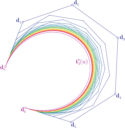
i.e., all combinations that appear in the order elevation process (10) are convex. This observation implies that the order elevated control polygon is closer to the shape of the curve than its original one. Therefore, repeatedly increasing the order of the trigonometric curve (7) from $n$ to $n+z$ ($z\geq 1$), we obtain a sequence of control polygons that converges to the curve generated by the starting control polygon. This geometric property is illustrated in Fig. 2 and it will be essential in case of control point based exact description of higher dimensional rational trigonometric curves and multivariate surfaces given in traditional parametric form.

Figure 2: A plane third order trigonometric curve ($\alpha=\frac{\pi}{2}$) with its original and order elevated control polygons which form a sequence that converges to the curve generated by the original control polygon.

Remark 2.5 (Asymptotic behavior)

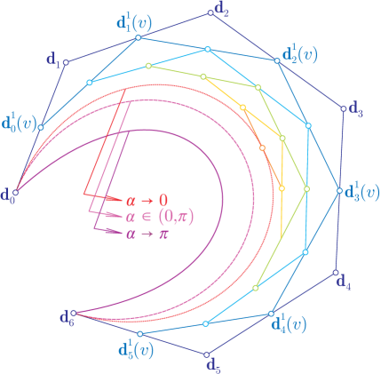
As proved in (JuhaszRoth2014, , Proposition 2.1, p. 249), the basis $\overline{\mathcal{T}}_{2n}^{\alpha}$ degenerates to the classical Bernstein polynomial basis $\mathcal{B}_{2n}$ defined over the unit compact interval as the shape parameter $\alpha$ tends to $0$ from above. In this case the trigonometric curve (7) becomes a classical Bézier curve of degree $2n$, while the subdivision algorithm presented in Remark 2.3 degenerates to the classical non-rational de Casteljau algorithm. Fig. 3 illustrates the effect of the shape parameter $\alpha\in\left(0,\pi\right)$ on the image of a third order trigonometric curve.

Figure 3: Effect of the design parameter $\alpha\in\left(0,\pi\right)$ on the shape of a third order trigonometric curve. In the limiting case $\alpha\rightarrow 0$ the curve becomes a classical Bézier curve of degree $6$ (as it is expected, in this special case, the B-algorithm of the trigonometric curve degenerates to the classical corner cutting de Casteljau algorithm, i.e., each subdivision point is determined by the same ratio along the edges of the control polygon.)

Definition 2.2 (Rational trigonometric curves)

The non-negative weight vector $\mathbf{\boldsymbol{\omega}}=\left[\omega_{i}\right]_{i=0}^{2n}$ of rank $1$ associated with the control polygon $\left[\mathbf{d}_{i}\right]_{i=0}^{2n}\in\mathcal{M}_{1,2n+1}\left(\mathbb{R}^{\delta}\right)$ and the normalized linearly independent rational (or quotient) functions

$$R_{2n,i}^{\alpha,\mathbf{\boldsymbol{\omega}}}\left(u\right)=\frac{\omega_{i}T_{2n,i}^{\alpha}\left(u\right)}{{\displaystyle\sum\limits_{j=0}^{2n}}\omega_{j}T_{2n,j}^{\alpha}\left(u\right)},~{}u\in\left[0,\alpha\right],~{}i=0,1,\ldots,2n$$

define the rational counterpart

$$\mathbf{t}_{n}^{\alpha,\mathbf{\boldsymbol{\omega}}}\left(u\right)=\sum_{i=0}^{2n}\omega_{i}\mathbf{d}_{i}R_{2n,i}^{\alpha,\mathbf{\boldsymbol{\omega}}}\left(u\right)=\frac{{\displaystyle\sum\limits_{i=0}^{2n}}\omega_{i}\mathbf{d}_{i}T_{2n,i}^{\alpha}\left(u\right)}{{\displaystyle\sum\limits_{j=0}^{2n}}\omega_{j}T_{2n,j}^{\alpha}\left(u\right)},~{}u\in\left[0,\alpha\right]$$ (11)

of the trigonometric curve (7).

Remark 2.6 (Pre-image of rational trigonometric curves)

The rational trigonometric curve (11) can also be considered as the central projection of the higher dimensional curve

$$\mathbf{t}_{n,\mathcal{\wp}}^{\alpha,\mathbf{\boldsymbol{\omega}}}\left(u\right)=\sum_{i=0}^{2n}\left[\begin{array}[c]{c}\omega_{i}\mathbf{d}_{i}\\ \omega_{i}\end{array}\right]T_{2n,i}^{\alpha}\left(u\right),~{}u\in\left[0,\alpha\right]$$ (12)

in the $\delta+1$ dimensional space from the origin onto the $\delta$ dimensional hyperplane $x^{\delta+1}=1$ (assuming that the coordinates of $\mathbb{R}^{\delta+1}$ are denoted by $x^{1},x^{2},\ldots,x^{\delta+1}$). The curve (12) is called the pre-image of the rational curve (11), while the vector space $\mathbb{R}^{\delta+1}$ is called its pre-image space. This concept will be useful in case of control point based exact description of smooth rational trigonometric curves given in traditional parametric form expressed in the canonical basis $\mathcal{T}_{2n}^{\alpha}$.

2.2 Hyperbolic curves and their rational counterpart

In this case, let $\alpha>0$ be an arbitrarily fixed parameter and consider the B-basis

$$\overline{\mathcal{H}}_{2n}^{\alpha}=\left\{H_{2n,i}^{\alpha}\left(u\right):u\in\left[0,\alpha\right]\right\}_{i=0}^{2n}=\left\{h_{2n,i}^{\alpha}\sinh^{2n-i}\left(\frac{\alpha-u}{2}\right)\sinh^{i}\left(\frac{u}{2}\right):u\in\left[0,\alpha\right]\right\}_{i=0}^{2n}$$ (13)

of order $n$ (degree $2n$) of the vector space (2) introduced in ShenWang2005 , where the non-negative normalizing coefficients

$$h_{2n,i}^{\alpha}=\frac{1}{\sinh^{2n}\left(\frac{\alpha}{2}\right)}\sum_{r=0}^{\left\lfloor\frac{i}{2}\right\rfloor}\binom{n}{i-r}\binom{i-r}{r}\left(2\cosh\left(\frac{\alpha}{2}\right)\right)^{i-2r},~{}i=0,1,\ldots,2n$$

fulfill the symmetry property

$$h_{2n,i}^{\alpha}=h_{2n,2n-i}^{\alpha},~{}i=0,1,\ldots,n\text{.}$$ (14)

Definition 2.3 (Hyperbolic curves)

The convex combination

$$\mathbf{h}_{n}^{\alpha}\left(u\right)=\sum_{i=0}^{2n}\mathbf{d}_{i}H_{2n,i}^{\alpha}\left(u\right),~{}u\in\left[0,\alpha\right],$$ (15)

defines a hyperbolic curve of order $n$ (degree $2n$), where $\left[\mathbf{d}_{i}\right]_{i=0}^{2n}\in\mathcal{M}_{1,2n+1}\left(\mathbb{R}^{\delta}\right)$ forms a control polygon.

Similarly to Subsection 2.1 it is easy to observe that curves of type (15) are in fact special reparametrizations of a class of rational Bézier curves of even degree $2n$. Instead of trigonometric sine, cosine, and tangent functions one has to apply the hyperbolic variant of these functions, i.e., instead of parameter transformation (8) and weights (9) one has to substitute the reparametrization function

$$\left\{\begin{array}[c]{l}v:\left[0,\alpha\right]\rightarrow\left[0,1\right],\\ \\ v\left(u\right)=\dfrac{1}{2}+\dfrac{\tanh\left(\frac{u}{2}-\frac{\alpha}{4}\right)}{2\tanh\left(\frac{\alpha}{4}\right)}=\dfrac{\sinh\left(\frac{u}{2}\right)}{2\cosh\left(\frac{\alpha}{4}-\frac{u}{2}\right)\sinh\left(\frac{\alpha}{4}\right)}\end{array}\right.$$ (16)

and weights

$$w_{i}=\frac{h_{2n,i}^{\alpha}}{\binom{2n}{i}},~{}i=0,1,\ldots,2n$$ (17)

into the rational Bézier curve (3), respectively.

Using observations similar to Remarks 2.3, 2.4 and 2.5, the subdivision, order elevation and asymptotic behavior of hyperbolic curves of type (15) can also be formulated. With the exception of the subdivision algorithm and without the observation of the parameter transformation (16) and special weight settings (17), the asymptotic behavior and the order elevation of hyperbolic curves were first studied in ShenWang2005 . The steps of the subdivision of a third order hyperbolic curve is presented in Fig. 1(b).

The rational variant of the hyperbolic curve (15) and its pre-image can also be easily described.

Definition 2.4 (Rational hyperbolic curves)

Consider the non-negative weight vector $\mathbf{\boldsymbol{\omega}}=\left[\omega_{i}\right]_{i=0}^{2n}$ of rank $1$ associated with the control polygon $\left[\mathbf{d}_{i}\right]_{i=0}^{2n}\in\mathcal{M}_{1,2n+1}\left(\mathbb{R}^{\delta}\right)$. Normalized quotient basis functions

$$S_{2n,i}^{\alpha,\mathbf{\boldsymbol{\omega}}}\left(u\right)=\frac{\omega_{i}H_{2n,i}^{\alpha}\left(u\right)}{{\displaystyle\sum\limits_{j=0}^{2n}}\omega_{j}H_{2n,j}^{\alpha}\left(u\right)},~{}u\in\left[0,\alpha\right],~{}i=0,1,\ldots,2n$$

generate the rational counterpart

$$\mathbf{h}_{n}^{\alpha,\mathbf{\boldsymbol{\omega}}}\left(u\right)=\sum_{i=0}^{2n}\omega_{i}\mathbf{d}_{i}S_{2n,i}^{\alpha,\mathbf{\boldsymbol{\omega}}}\left(u\right)=\frac{{\displaystyle\sum\limits_{i=0}^{2n}}\omega_{i}\mathbf{d}_{i}H_{2n,i}^{\alpha}\left(u\right)}{{\displaystyle\sum\limits_{j=0}^{2n}}\omega_{j}H_{2n,j}^{\alpha}\left(u\right)},~{}u\in\left[0,\alpha\right]$$ (18)

of the hyperbolic curve (15), the pre-image of which is

$$\mathbf{h}_{n,\mathcal{\wp}}^{\alpha,\mathbf{\boldsymbol{\omega}}}\left(u\right)=\sum_{i=0}^{2n}\left[\begin{array}[c]{c}\omega_{i}\mathbf{d}_{i}\\ \omega_{i}\end{array}\right]H_{2n,i}^{\alpha}\left(u\right),~{}u\in\left[0,\alpha\right].$$ (19)

3 (Hybrid) (rational) trigonometric and hyperbolic multivariate surfaces

By means of tensor products of curves of type (7) and (15) one can introduce the following multivariate higher dimensional surface modeling tools. Let $\delta\geq 2$ and $\kappa\geq 0$ arbitrarily fixed natural numbers and consider the also fixed vector $\mathbf{n}=\left[n_{j}\right]_{j=1}^{\delta}$ of orders, where $n_{j}\geq 1$ for all $j=1,2,\ldots,\delta$.

Definition 3.5 (Trigonometric surfaces and their rational counterpart)

Let

$$\mathbf{\boldsymbol{\alpha}=}\left[\alpha_{j}\right]_{j=1}^{\delta}\in\times_{j=1}^{\delta}\left(0,\pi\right)$$

be a fixed vector of shape parameters and consider the multidimensional control grid

$$\left[\mathbf{d}_{i_{1},i_{2},\ldots,i_{\delta}}\right]_{i_{1}=0,i_{2}=0,\ldots,i_{\delta}=0}^{2n_{1},2n_{2},\ldots,2n_{\delta}}\in\mathcal{M}_{2n_{1}+1,2n_{2}+1,\ldots 2n_{\delta}+1}\left(\mathbb{R}^{\delta+\kappa}\right).$$ (20)

The multivariate surface

$$\mathbf{t}_{\mathbf{n}}^{\mathbf{\boldsymbol{\alpha}}}\left(\mathbf{u}\right) =\mathbf{t}_{n_{1},n_{2},\ldots,n_{\delta}}^{\alpha_{1},\alpha_{2},\ldots,\alpha_{\delta}}\left(u_{1},u_{2},\ldots,u_{\delta}\right)$$ (21)

$$=\sum_{i_{1}=0}^{2n_{1}}\sum_{i_{2}=0}^{2n_{2}}\cdots\sum_{i_{\delta}=0}^{2n_{\delta}}\mathbf{d}_{i_{1},i_{2},\ldots,i_{\delta}}T_{2n_{1},i_{1}}^{\alpha_{1}}\left(u_{1}\right)T_{2n_{2},i_{2}}^{\alpha_{2}}\left(u_{2}\right)\cdot\ldots\cdot T_{2n_{\delta},i_{\delta}}^{\alpha_{\delta}}\left(u_{\delta}\right),~{}\mathbf{u}=\left[u_{j}\right]_{j=1}^{\delta}\in\times_{j=1}^{\delta}\left[0,\alpha_{j}\right]$$

is called $\delta$-variate trigonometric surface of order $\mathbf{n}$ taking values in $\mathbb{R}^{\delta+\kappa}$. Assigning the non-negative multidimensional weight matrix

$$\boldsymbol{\Omega}=\left[\omega_{i_{1},i_{2},\ldots,i_{\delta}}\right]_{i_{1}=0,i_{2}=0,\ldots,i_{\delta}=0}^{2n_{1},2n_{2},\ldots,2n_{\delta}}\in\mathcal{M}_{2n_{1}+1,2n_{2}+1,\ldots 2n_{\delta}+1}\left(\mathbb{R}_{+}\right)$$ (22)

of rank at least $1$ to the control grid (20), one obtains the $\delta$-variate rational trigonometric surface

$$\mathbf{t}_{\mathbf{n}}^{\mathbf{\boldsymbol{\alpha}},\boldsymbol{\Omega}}\left(\mathbf{u}\right) =\mathbf{t}_{n_{1},n_{2},\ldots,n_{\delta}}^{\alpha_{1},\alpha_{2},\ldots,\alpha_{\delta},\boldsymbol{\Omega}}\left(u_{1},u_{2},\ldots,u_{\delta}\right)$$ (23)

$$=\frac{{\displaystyle\sum\limits_{i_{1}=0}^{2n_{1}}}{\displaystyle\sum\limits_{i_{2}=0}^{2n_{2}}}\cdots{\displaystyle\sum\limits_{i_{\delta}=0}^{2n_{\delta}}}\omega_{i_{1},i_{2},\ldots,i_{\delta}}\mathbf{d}_{i_{1},i_{2},\ldots,i_{\delta}}T_{2n_{1},i_{1}}^{\alpha_{1}}\left(u_{1}\right)T_{2n_{2},i_{2}}^{\alpha_{2}}\left(u_{2}\right)\cdot\ldots\cdot T_{2n_{\delta},i_{\delta}}^{\alpha_{\delta}}\left(u_{\delta}\right)}{{\displaystyle\sum\limits_{j_{1}=0}^{2n_{1}}}{\displaystyle\sum\limits_{j_{2}=0}^{2n_{2}}}\cdots{\displaystyle\sum\limits_{j_{\delta}=0}^{2n_{\delta}}}\omega_{j_{1},j_{2},\ldots,j_{\delta}}T_{2n_{1},j_{1}}^{\alpha_{1}}\left(u_{1}\right)T_{2n_{2},j_{2}}^{\alpha_{2}}\left(u_{2}\right)\cdot\ldots\cdot T_{2n_{\delta},j_{\delta}}^{\alpha_{\delta}}\left(u_{\delta}\right)}$$

of the same order, which is the central projection of the pre-image

$$\mathbf{t}_{\mathbf{n},\wp}^{\mathbf{\boldsymbol{\alpha}},\boldsymbol{\Omega}}\left(\mathbf{u}\right) =\mathbf{t}_{n_{1},n_{2},\ldots,n_{\delta},\wp}^{\alpha_{1},\alpha_{2},\ldots,\alpha_{\delta},\boldsymbol{\Omega}}\left(u_{1},u_{2},\ldots,u_{\delta}\right)$$ (24)

$$=\sum_{i_{1}=0}^{2n_{1}}\sum_{i_{2}=0}^{2n_{2}}\cdots\sum_{i_{\delta}=0}^{2n_{\delta}}\left[\begin{array}[c]{c}\omega_{i_{1},i_{2},\ldots,i_{\delta}}\mathbf{d}_{i_{1},i_{2},\ldots,i_{\delta}}\\ \omega_{i_{1},i_{2},\ldots,i_{\delta}}\end{array}\right]T_{2n_{1},i_{1}}^{\alpha_{1}}\left(u_{1}\right)T_{2n_{2},i_{2}}^{\alpha_{2}}\left(u_{2}\right)\cdot\ldots\cdot T_{2n_{\delta},i_{\delta}}^{\alpha_{\delta}}\left(u_{\delta}\right)$$ (27)

in $\mathbb{R}^{\delta+\kappa+1}$ from its origin onto the $\delta+\kappa$ dimensional hyperplane $x^{\delta+k+1}=1$ (provided that the coordinates of $\mathbb{R}^{\delta+\kappa+1}$ are labeled by $x^{1},x^{2},\ldots,x^{\delta+k+1}$).

Remark 3.7 ($3$-dimensional $2$-variate trigonometric surfaces)

The simplest variant of multivariate surfaces introduced in Definition 3.5 corresponds to $\delta=2$ and $\kappa=1$, when the $2$-variate trigonometric surface (21) is a $3$-dimensional traditional tensor product surface of curves of the type (7). In this special case, the grid (20) of control points and the multidimensional weight matrix (22) degenerate to a traditional control net and rectangular weight matrix, respectively.

Remark 3.8 ($3$-dimensional trigonometric volumes)

Using settings $\delta=3$ and $\kappa=0$, Definition 3.5 describes $3$-dimensional volumes (solids) by means of $3$-variate tensor product of curves of the type (7).

Definition 3.6 (Hyperbolic surfaces and their rational counterpart)

Let

$$\mathbf{\boldsymbol{\alpha}=}\left[\alpha_{j}\right]_{j=1}^{\delta}\in\times_{j=1}^{\delta}\left(0,+\infty\right)$$

be a fixed vector of shape parameters and consider the non-negative multidimensional weight matrix

$$\boldsymbol{\Omega}=\left[\omega_{i_{1},i_{2},\ldots,i_{\delta}}\right]_{i_{1}=0,i_{2}=0,\ldots,i_{\delta}=0}^{2n_{1},2n_{2},\ldots,2n_{\delta}}\in\mathcal{M}_{2n_{1}+1,2n_{2}+1,\ldots 2n_{\delta}+1}\left(\mathbb{R}_{+}\right)$$

(of rank at least $1$) associated with the control grid

$$\left[\mathbf{d}_{i_{1},i_{2},\ldots,i_{\delta}}\right]_{i_{1}=0,i_{2}=0,\ldots,i_{\delta}=0}^{2n_{1},2n_{2},\ldots,2n_{\delta}}\in\mathcal{M}_{2n_{1}+1,2n_{2}+1,\ldots 2n_{\delta}+1}\left(\mathbb{R}^{\delta+\kappa}\right).$$

The multivariate hyperbolic surface of order $\mathbf{n}$, its rational counterpart, and the pre-image of the rational variant are

$$\mathbf{h}_{\mathbf{n}}^{\mathbf{\boldsymbol{\alpha}}}\left(\mathbf{u}\right) =\mathbf{h}_{n_{1},n_{2},\ldots,n_{\delta}}^{\alpha_{1},\alpha_{2},\ldots,\alpha_{\delta}}\left(u_{1},u_{2},\ldots,u_{\delta}\right)$$ (28)

$$=\sum_{i_{1}=0}^{2n_{1}}\sum_{i_{2}=0}^{2n_{2}}\cdots\sum_{i_{\delta}=0}^{2n_{\delta}}\mathbf{d}_{i_{1},i_{2},\ldots,i_{\delta}}H_{2n_{1},i_{1}}^{\alpha_{1}}\left(u_{1}\right)H_{2n_{2},i_{2}}^{\alpha_{2}}\left(u_{2}\right)\cdot\ldots\cdot H_{2n_{\delta},i_{\delta}}^{\alpha_{\delta}}\left(u_{\delta}\right),$$

$$\mathbf{u} =\left[u_{j}\right]_{j=1}^{\delta}\in\times_{j=1}^{\delta}\left[0,\alpha_{j}\right],$$

$$\mathbf{h}_{\mathbf{n}}^{\mathbf{\boldsymbol{\alpha}},\boldsymbol{\Omega}}\left(\mathbf{u}\right) =\mathbf{h}_{n_{1},n_{2},\ldots,n_{\delta}}^{\alpha_{1},\alpha_{2},\ldots,\alpha_{\delta},\boldsymbol{\Omega}}\left(u_{1},u_{2},\ldots,u_{\delta}\right)$$ (29)

$$=\frac{{\displaystyle\sum\limits_{i_{1}=0}^{2n_{1}}}{\displaystyle\sum\limits_{i_{2}=0}^{2n_{2}}}\cdots{\displaystyle\sum\limits_{i_{\delta}=0}^{2n_{\delta}}}\omega_{i_{1},i_{2},\ldots,i_{\delta}}\mathbf{d}_{i_{1},i_{2},\ldots,i_{\delta}}H_{2n_{1},i_{1}}^{\alpha_{1}}\left(u_{1}\right)H_{2n_{2},i_{2}}^{\alpha_{2}}\left(u_{2}\right)\cdot\ldots\cdot H_{2n_{\delta},i_{\delta}}^{\alpha_{\delta}}\left(u_{\delta}\right)}{{\displaystyle\sum\limits_{j_{1}=0}^{2n_{1}}}{\displaystyle\sum\limits_{j_{2}=0}^{2n_{2}}}\cdots{\displaystyle\sum\limits_{j_{\delta}=0}^{2n_{\delta}}}\omega_{j_{1},j_{2},\ldots,j_{\delta}}H_{2n_{1},j_{1}}^{\alpha_{1}}\left(u_{1}\right)H_{2n_{2},j_{2}}^{\alpha_{2}}\left(u_{2}\right)\cdot\ldots\cdot H_{2n_{\delta},j_{\delta}}^{\alpha_{\delta}}\left(u_{\delta}\right)}$$

and

$$\mathbf{h}_{\mathbf{n},\wp}^{\mathbf{\boldsymbol{\alpha}},\boldsymbol{\Omega}}\left(\mathbf{u}\right) =\mathbf{h}_{n_{1},n_{2},\ldots,n_{\delta},\wp}^{\alpha_{1},\alpha_{2},\ldots,\alpha_{\delta},\boldsymbol{\Omega}}\left(u_{1},u_{2},\ldots,u_{\delta}\right)$$

$$=\sum_{i_{1}=0}^{2n_{1}}\sum_{i_{2}=0}^{2n_{2}}\cdots\sum_{i_{\delta}=0}^{2n_{\delta}}\left[\begin{array}[c]{c}\omega_{i_{1},i_{2},\ldots,i_{\delta}}\mathbf{d}_{i_{1},i_{2},\ldots,i_{\delta}}\\ \omega_{i_{1},i_{2},\ldots,i_{\delta}}\end{array}\right]H_{2n_{1},i_{1}}^{\alpha_{1}}\left(u_{1}\right)H_{2n_{2},i_{2}}^{\alpha_{2}}\left(u_{2}\right)\cdot\ldots\cdot H_{2n_{\delta},i_{\delta}}^{\alpha_{\delta}}\left(u_{\delta}\right),$$

respectively.

Remark 3.9 (Hybrid multivariate surfaces)

Naturally, one can also mix the trigonometric or hyperbolic type of B-basis functions in directions $\left[u_{j}\right]_{j=1}^{\delta}$, i.e., one can also define higher dimensional hybrid multivariate (rational) surfaces.

4 Basis transformations

We are going to derive recursive formulae for the transformation of B-bases $\overline{\mathcal{T}}_{2n}^{\alpha}$ and $\overline{\mathcal{H}}_{2n}^{\alpha}$ to the canonical bases $\mathcal{T}_{2n}^{\alpha}$ and $\mathcal{H}_{2n}^{\alpha}$ of the vector spaces $\mathbb{T}_{2n}^{\alpha}$ and $\mathbb{H}_{2n}^{\alpha}$, respectively.

4.1 The trigonometric case

Let $k\in\left\{0,1,\ldots,n\right\}$ be an arbitrarily fixed natural number. Assume that the unique representations of trigonometric functions $\sin\left(ku\right)$ and $\cos\left(ku\right)$ in the basis (5) of order $n$ are

$$\sin\left(ku\right)=\sum_{i=0}^{2n}\lambda_{k,i}^{n}T_{2n,i}^{\alpha}\left(u\right),~{}u\in\left[0,\alpha\right]$$ (30)

and

$$\cos\left(ku\right)=\sum_{i=0}^{2n}\mu_{k,i}^{n}T_{2n,i}^{\alpha}\left(u\right),~{}u\in\left[0,\alpha\right],$$ (31)

respectively, where coefficients $\left\{\lambda_{k,i}^{n}\right\}_{i=0}^{2n}$ and $\left\{\mu_{k,i}^{n}\right\}_{i=0}^{2n}$ are unique real numbers. The basis transformation from the first order B-basis $\overline{\mathcal{T}}_{2}^{\alpha}$ to the first order trigonometric canonical basis $\mathcal{T}_{2}^{\alpha}$ can be expressed in the matrix form

$$\left[\begin{array}[c]{c}1\\ \sin\left(u\right)\\ \cos\left(u\right)\end{array}\right]=\left[\begin{array}[c]{ccc}\mu_{0,0}^{1}&\mu_{0,1}^{1}&\mu_{0,2}^{1}\\ \lambda_{1,0}^{1}&\lambda_{1,1}^{1}&\lambda_{1,2}^{1}\\ \mu_{1,0}^{1}&\mu_{1,1}^{1}&\mu_{1,2}^{1}\end{array}\right]\left[\begin{array}[c]{c}T_{2,0}^{\alpha}\left(u\right)\\ T_{2,1}^{\alpha}\left(u\right)\\ T_{2,2}^{\alpha}\left(u\right)\end{array}\right],~{}\forall u\in\left[0,\alpha\right],$$

where

$$\left\{\begin{array}[c]{l}\mu_{0,0}^{1}=\mu_{0,1}^{1}=\mu_{0,2}^{1}=1,\\ \\ \lambda_{1,0}^{1}=0,~{}\lambda_{1,1}^{1}=\tan\left(\frac{\alpha}{2}\right),~{}\lambda_{1,2}^{1}=\sin\left(\alpha\right),\\ \\ \mu_{1,0}^{1}=\mu_{1,1}^{1}=1,~{}\mu_{1,2}^{1}=\cos\left(\alpha\right).\end{array}\right.$$ (32)

Using initial conditions (32), our objective is to derive recursive formulae for the matrix elements of the linear transformation that changes the higher order B-basis $\overline{\mathcal{T}}_{2\left(n+1\right)}^{\alpha}$ to the canonical trigonometric basis $\mathcal{T}_{2\left(n+1\right)}^{\alpha}$.

Performing order elevation on functions (30) and (31), one obtains that

$$\sin\left(ku\right)=\sum_{r=0}^{2\left(n+1\right)}\lambda_{k,r}^{n+1}T_{2\left(n+1\right),r}^{\alpha}\left(u\right)$$

and

$$\cos\left(ku\right)=\sum_{r=0}^{2\left(n+1\right)}\mu_{k,r}^{n+1}T_{2\left(n+1\right),r}^{\alpha}\left(u\right),$$

where

$$\lambda_{k,0}^{n+1} =\lambda_{k,0}^{n},$$

$$\lambda_{k,1}^{n+1} =\lambda_{k,0}^{n}\frac{t_{2n,0}^{\alpha}t_{2,1}^{\alpha}}{t_{2\left(n+1\right),1}^{\alpha}}+\lambda_{k,1}^{n}\frac{t_{2n,1}^{\alpha}t_{2,0}^{\alpha}}{t_{2\left(n+1\right),1}^{\alpha}},$$

$$\lambda_{k,r}^{n+1} =\lambda_{k,r-2}^{n}\frac{t_{2n,r-2}^{\alpha}t_{2,2}^{\alpha}}{t_{2\left(n+1\right),r}^{\alpha}}+\lambda_{k,r-1}^{n}\frac{t_{2n,r-1}^{\alpha}t_{2,1}^{\alpha}}{t_{2\left(n+1\right),r}^{\alpha}}+\lambda_{k,r}^{n}\frac{t_{2n,r}^{\alpha}t_{2,0}^{\alpha}}{t_{2\left(n+1\right),r}^{\alpha}},~{}r=2,3,\ldots,2n,$$

$$\lambda_{k,2n+1}^{n+1} =\lambda_{k,2n-1}^{n}\frac{t_{2n,2n-1}^{\alpha}t_{2,2}^{\alpha}}{t_{2\left(n+1\right),2n+1}^{\alpha}}+\lambda_{k,2n}^{n}\frac{t_{2n,2n}^{\alpha}t_{2,1}^{\alpha}}{t_{2\left(n+1\right),2n+1}^{\alpha}},$$

$$\lambda_{k,2\left(n+1\right)}^{n+1} =\lambda_{k,2n}^{n}$$

and

$$\mu_{k,0}^{n+1} =\mu_{k,0}^{n},$$

$$\mu_{k,1}^{n+1} =\mu_{k,0}^{n}\frac{t_{2n,0}^{\alpha}t_{2,1}^{\alpha}}{t_{2\left(n+1\right),1}^{\alpha}}+\mu_{k,1}^{n}\frac{t_{2n,1}^{\alpha}t_{2,0}^{\alpha}}{t_{2\left(n+1\right),1}^{\alpha}},$$

$$\mu_{k,r}^{n+1} =\mu_{k,r-2}^{n}\frac{t_{2n,r-2}^{\alpha}t_{2,2}^{\alpha}}{t_{2\left(n+1\right),r}^{\alpha}}+\mu_{k,r-1}^{n}\frac{t_{2n,r-1}^{\alpha}t_{2,1}^{\alpha}}{t_{2\left(n+1\right),r}^{\alpha}}+\mu_{k,r}^{n}\frac{t_{2n,r}^{\alpha}t_{2,0}^{\alpha}}{t_{2\left(n+1\right),r}^{\alpha}},~{}r=2,3,\ldots,2n,$$

$$\mu_{k,2n+1}^{n+1} =\mu_{k,2n-1}^{n}\frac{t_{2n,2n-1}^{\alpha}t_{2,2}^{\alpha}}{t_{2\left(n+1\right),2n+1}^{\alpha}}+\mu_{k,2n}^{n}\frac{t_{2n,2n}^{\alpha}t_{2,1}^{\alpha}}{t_{2\left(n+1\right),2n+1}^{\alpha}},$$

$$\mu_{k,2\left(n+1\right)}^{n+1} =\mu_{k,2n}^{n},$$

respectively. Moreover, due to initial conditions (32) and simple trigonometric identities

$$\sin\left(a+b\right) =\sin\left(a\right)\cos\left(b\right)+\cos\left(a\right)\sin\left(b\right),$$ (33)

$$\cos\left(a+b\right) =\cos\left(a\right)\cos\left(b\right)-\sin\left(a\right)\sin\left(b\right),$$ (34)

one has that

$$\sin\left(\left(n+1\right)u\right) =\left(\sum_{i=0}^{2n}\lambda_{n,i}^{n}T_{2n,i}^{\alpha}\left(u\right)\right)\left(\sum_{j=0}^{2}\mu_{1,j}^{1}T_{2,j}^{\alpha}\left(u\right)\right)+\left(\sum_{i=0}^{2n}\mu_{n,i}^{n}T_{2n,i}^{\alpha}\left(u\right)\right)\left(\sum_{j=0}^{2}\lambda_{1,j}^{1}T_{2,j}^{\alpha}\left(u\right)\right)$$

$$=\sum_{r=0}^{2\left(n+1\right)}\lambda_{n+1,r}^{n+1}T_{2\left(n+1\right),r}^{\alpha}\left(u\right),$$

$$\cos\left(\left(n+1\right)u\right) =\left(\sum_{i=0}^{2n}\mu_{n,i}^{n}T_{2n,i}^{\alpha}\left(u\right)\right)\left(\sum_{j=0}^{2}\mu_{1,j}^{1}T_{2,j}^{\alpha}\left(u\right)\right)-\left(\sum_{i=0}^{2n}\lambda_{n,i}^{n}T_{2n,i}^{\alpha}\left(u\right)\right)\left(\sum_{j=0}^{2}\lambda_{1,j}^{1}T_{2,j}^{\alpha}\left(u\right)\right)$$

$$=\sum_{r=0}^{2\left(n+1\right)}\mu_{n+1,r}^{n+1}T_{2\left(n+1\right),r}^{\alpha}\left(u\right),$$

where

$$\lambda_{n+1,0}^{n+1}= \lambda_{n,0}^{n}\mu_{1,0}^{1}+\mu_{n,0}^{n}\lambda_{1,0}^{1},$$

$$\lambda_{n+1,1}^{n+1}= \left(\lambda_{n,0}^{n}\mu_{1,1}^{1}+\mu_{n,0}^{n}\lambda_{1,1}^{1}\right)\frac{t_{2n,0}^{\alpha}t_{2,1}^{\alpha}}{t_{2\left(n+1\right),1}^{\alpha}}+\left(\lambda_{n,1}^{n}\mu_{1,0}^{1}+\mu_{n,1}^{n}\lambda_{1,0}^{1}\right)\frac{t_{2n,1}^{\alpha}t_{2,0}^{\alpha}}{t_{2\left(n+1\right),1}^{\alpha}},$$

$$\lambda_{n+1,r}^{n+1}= \left(\lambda_{n,r-2}^{n}\mu_{1,2}^{1}+\mu_{n,r-2}^{n}\lambda_{1,2}^{1}\right)\frac{t_{2n,r-2}^{\alpha}t_{2,2}^{\alpha}}{t_{2\left(n+1\right),r}^{\alpha}}+\left(\lambda_{n,r-1}^{n}\mu_{1,1}^{1}+\mu_{n,r-1}^{n}\lambda_{1,1}^{1}\right)\frac{t_{2n,r-1}^{\alpha}t_{2,1}^{\alpha}}{t_{2\left(n+1\right),r}^{\alpha}}$$

$$+\left(\lambda_{n,r}^{n}\mu_{1,0}^{1}+\mu_{n,r}^{n}\lambda_{1,0}^{1}\right)\frac{t_{2n,r}^{\alpha}t_{2,0}^{\alpha}}{t_{2\left(n+1\right),r}^{\alpha}},~{}r=2,3,\ldots,2n,$$

$$\lambda_{n+1,2n+1}^{n+1}= \left(\lambda_{n,2n-1}^{n}\mu_{1,2}^{1}+\mu_{n,2n-1}^{n}\lambda_{1,2}^{1}\right)\frac{t_{2n,2n-1}^{\alpha}t_{2,2}^{\alpha}}{t_{2\left(n+1\right),2n+1}^{\alpha}}+\left(\lambda_{n,2n}^{n}\mu_{1,1}^{1}+\mu_{n,2n}^{n}\lambda_{1,1}^{1}\right)\frac{t_{2n,2n}^{\alpha}t_{2,1}^{\alpha}}{t_{2\left(n+1\right),2n+1}^{\alpha}},$$

$$\lambda_{n+1,2\left(n+1\right)}^{n+1}= \lambda_{n,2n}^{n}\mu_{1,2}^{1}+\mu_{n,2n}^{n}\lambda_{1,2}^{1}$$

and

$$\mu_{n+1,0}^{n+1}= \mu_{n,0}^{n}\mu_{1,0}^{1}-\lambda_{n,0}^{n}\lambda_{1,0}^{1},$$

$$\mu_{n+1,1}^{n+1}= \left(\mu_{n,0}^{n}\mu_{1,1}^{1}-\lambda_{n,0}^{n}\lambda_{1,1}^{1}\right)\frac{t_{2n,0}^{\alpha}t_{2,1}^{\alpha}}{t_{2\left(n+1\right),1}^{\alpha}}+\left(\mu_{n,1}^{n}\mu_{1,0}^{1}-\lambda_{n,1}^{n}\lambda_{1,0}^{1}\right)\frac{t_{2n,1}^{\alpha}t_{2,0}^{\alpha}}{t_{2\left(n+1\right),1}^{\alpha}},$$

$$\mu_{n+1,r}^{n+1}= \left(\mu_{n,r-2}^{n}\mu_{1,2}^{1}-\lambda_{n,r-2}^{n}\lambda_{1,2}^{1}\right)\frac{t_{2n,r-2}^{\alpha}t_{2,2}^{\alpha}}{t_{2\left(n+1\right),r}^{\alpha}}+\left(\mu_{n,r-1}^{n}\mu_{1,1}^{1}-\lambda_{n,r-1}^{n}\lambda_{1,1}^{1}\right)\frac{t_{2n,r-1}^{\alpha}t_{2,1}^{\alpha}}{t_{2\left(n+1\right),r}^{\alpha}}$$

$$+\left(\mu_{n,r}^{n}\mu_{1,0}^{1}-\lambda_{n,r}^{n}\lambda_{1,0}^{1}\right)\frac{t_{2n,r}^{\alpha}t_{2,0}^{\alpha}}{t_{2\left(n+1\right),r}^{\alpha}},~{}r=2,3,\ldots,2n,$$

$$\mu_{n+1,2n+1}^{n+1}= \left(\mu_{n,2n-1}^{n}\mu_{1,2}^{1}-\lambda_{n,2n-1}^{n}\lambda_{1,2}^{1}\right)\frac{t_{2n,2n-1}^{\alpha}t_{2,2}^{\alpha}}{t_{2\left(n+1\right),2n+1}^{\alpha}}+\left(\mu_{n,2n}^{n}\mu_{1,1}^{1}-\lambda_{n,2n}^{n}\lambda_{1,1}^{1}\right)\frac{t_{2n,2n}^{\alpha}t_{2,1}^{\alpha}}{t_{2\left(n+1\right),2n+1}^{\alpha}},$$

$$\mu_{n+1,2\left(n+1\right)}^{n+1}= \mu_{n,2n}^{n}\mu_{1,2}^{1}-\lambda_{n,2n}^{n}\lambda_{1,2}^{1},$$

respectively. Summarizing all calculations above, we have proved the next theorem.

Theorem 4.1 (Trigonometric basis transformation)

The matrix form of the linear transformation from the normalized B-basis $\overline{\mathcal{T}}_{2\left(n+1\right)}^{\alpha}$ to the canonical trigonometric basis $\mathcal{T}_{2\left(n+1\right)}^{\alpha}$ is

$$\left[\begin{array}[c]{c}1\\ \sin\left(u\right)\\ \cos\left(u\right)\\ \vdots\\ \sin\left(\left(n+1\right)u\right)\\ \cos\left(\left(n+1\right)u\right)\end{array}\right]=\left[\begin{array}[c]{cccccc}1&1&1&\cdots&1&1\\ \lambda_{1,0}^{n+1}&\lambda_{1,1}^{n+1}&\lambda_{1,2}^{n+1}&\cdots&\lambda_{1,2n+1}^{n+1}&\lambda_{1,2\left(n+1\right)}^{n+1}\\ \mu_{1,0}^{n+1}&\mu_{1,1}^{n+1}&\mu_{1,2}^{n+1}&\cdots&\mu_{1,2n+1}^{n+1}&\mu_{1,2\left(n+1\right)}^{n+1}\\ \vdots&\vdots&\vdots&&\vdots&\vdots\\ \lambda_{n+1,0}^{n+1}&\lambda_{n+1,1}^{n+1}&\lambda_{n+1,2}^{n+1}&\cdots&\lambda_{n+1,2n+1}^{n+1}&\lambda_{n+1,2\left(n+1\right)}^{n+1}\\ \mu_{n+1,0}^{n+1}&\mu_{n+1,1}^{n+1}&\mu_{n+1,2}^{n+1}&\cdots&\mu_{n+1,2n+1}^{n+1}&\mu_{n+1,2\left(n+1\right)}^{n+1}\end{array}\right]\left[\begin{array}[c]{c}T_{2\left(n+1\right),0}^{\alpha}\left(u\right)\\ T_{2\left(n+1\right),1}^{\alpha}\left(u\right)\\ T_{2\left(n+1\right),2}^{\alpha}\left(u\right)\\ \vdots\\ T_{2\left(n+1\right),2n+1}^{\alpha}\left(u\right)\\ T_{2\left(n+1\right),2\left(n+1\right)}^{\alpha}\left(u\right)\end{array}\right]$$

for all parameters $u\in\left[0,\alpha\right]$.

Remark 4.10

The matrix of the $\left(n+1\right)$th order basis transformation that appears in Theorem 4.1 can be efficiently calculated by parallel programming since its rows and their entries are independent of each other. Based on the entries of the first and $n$th order transformation matrices that are already calculated in previous steps, each thread block has to build up a single row of the $\left(n+1\right)$th order basis transformation matrix, while each thread within a block has to calculate a single entry of the corresponding row.

4.2 The hyperbolic case

In this case we can proceed as in Subsection 4.1. Naturally, instead of trigonometric sine, cosine, tangent functions and identities (33) and (34) one has to apply the hyperbolic variant of these functions and identities, respectively. The only difference consists in a sign change in the hyperbolic counterpart of the identity (34), since

$$\cosh\left(a+b\right)=\cosh\left(a\right)\cosh\left(b\right)+\sinh\left(a\right)\sinh\left(b\right).$$ (35)

Let $k\in\left\{0,1,\ldots,n\right\}$ be an arbitrarily fixed natural number and denote the representations of hyperbolic functions $\sinh\left(ku\right)$ and $\cosh\left(ku\right)$ in the B-basis (13) by

$$\sinh\left(ku\right)=\sum_{i=0}^{2n}\sigma_{k,i}^{n}H_{2n,i}^{\alpha}\left(u\right),~{}u\in\left[0,\alpha\right]$$ (36)

and

$$\cosh\left(ku\right)=\sum_{i=0}^{2n}\rho_{k,i}^{n}H_{2n,i}^{\alpha}\left(u\right),~{}u\in\left[0,\alpha\right]$$ (37)

respectively, where coefficients $\left\{\sigma_{k,i}^{n}\right\}_{i=0}^{2n}$ and $\left\{\rho_{k,i}^{n}\right\}_{i=0}^{2n}$ are unique scalars. The basis transformation from the first order B-basis $\overline{\mathcal{H}}_{2}^{\alpha}$ to the first order hyperbolic canonical basis $\mathcal{H}_{2}^{\alpha}$ can be written in the matrix form

$$\left[\begin{array}[c]{c}1\\ \sinh\left(u\right)\\ \cosh\left(u\right)\end{array}\right]=\left[\begin{array}[c]{ccc}\rho_{0,0}^{1}&\rho_{0,1}^{1}&\rho_{0,2}^{1}\\ \sigma_{1,0}^{1}&\sigma_{1,1}^{1}&\sigma_{1,2}^{1}\\ \rho_{1,0}^{1}&\rho_{1,1}^{1}&\rho_{1,2}^{1}\end{array}\right]\left[\begin{array}[c]{c}H_{2,0}^{\alpha}\left(u\right)\\ H_{2,1}^{\alpha}\left(u\right)\\ H_{2,2}^{\alpha}\left(u\right)\end{array}\right],~{}\forall u\in\left[0,\alpha\right],$$

where

$$\left\{\begin{array}[c]{l}\rho_{0,0}^{1}=\rho_{0,1}^{1}=\rho_{0,2}^{1}=1,\\ \\ \sigma_{1,0}^{1}=0,~{}\sigma_{1,1}^{1}=\tanh\left(\frac{\alpha}{2}\right),~{}\sigma_{1,2}^{1}=\sinh\left(\alpha\right),\\ \\ \rho_{1,0}^{1}=\rho_{1,1}^{1}=1,~{}\rho_{1,2}^{1}=\cosh\left(\alpha\right).\end{array}\right.$$ (38)

Using initial conditions (38) and normalizing constants $\left[h_{2,j}^{\alpha}\right]_{j=0}^{2},\left[h_{2n,i}^{\alpha}\right]_{i=0}^{2n}$ and $\left[h_{2\left(n+1\right),r}^{\alpha}\right]_{r=0}^{2\left(n+1\right)}$ instead of $\left[t_{2,j}^{\alpha}\right]_{j=0}^{2},\left[t_{2n,i}^{\alpha}\right]_{i=0}^{2n}$ and $\left[t_{2\left(n+1\right),r}^{\alpha}\right]_{r=0}^{2\left(n+1\right)}$, respectively, one obtains recursive formulae for the unique order elevated coefficients $\left[\sigma_{k,r}^{n+1}\right]_{k=0,r=0}^{n+1,2\left(n+1\right)}$ and $\left[\rho_{k,r}^{n+1}\right]_{k=0,r=0}^{n,2\left(n+1\right)}$ in a similar way as it was done in the trigonometric case for constants $\left[\lambda_{k,r}^{n+1}\right]_{k=0,r=0}^{n+1,2\left(n+1\right)}$ and $\left[\mu_{k,r}^{n+1}\right]_{k=0,r=0}^{n,2\left(n+1\right)}$, respectively, while applying identity (35) for constants $\left[\rho_{n+1,r}^{n+1}\right]_{r=0}^{2\left(n+1\right)}$ we have that

$$\rho_{n+1,0}^{n+1}= \rho_{n,0}^{n}\rho_{1,0}^{1}+\sigma_{n,0}^{n}\sigma_{1,0}^{1},$$

$$\rho_{n+1,1}^{n+1}= \left(\rho_{n,0}^{n}\rho_{1,1}^{1}+\sigma_{n,0}^{n}\sigma_{1,1}^{1}\right)\frac{h_{2n,0}^{\alpha}h_{2,1}^{\alpha}}{h_{2\left(n+1\right),1}^{\alpha}}+\left(\rho_{n,1}^{n}\rho_{1,0}^{1}+\sigma_{n,1}^{n}\sigma_{1,0}^{1}\right)\frac{h_{2n,1}^{\alpha}h_{2,0}^{\alpha}}{h_{2\left(n+1\right),1}^{\alpha}},$$

$$\rho_{n+1,r}^{n+1}= \left(\rho_{n,r-2}^{n}\rho_{1,2}^{1}+\sigma_{n,r-2}^{n}\sigma_{1,2}^{1}\right)\frac{h_{2n,r-2}^{\alpha}h_{2,2}^{\alpha}}{h_{2\left(n+1\right),r}^{\alpha}}+\left(\rho_{n,r-1}^{n}\rho_{1,1}^{1}+\sigma_{n,r-1}^{n}\sigma_{1,1}^{1}\right)\frac{h_{2n,r-1}^{\alpha}h_{2,1}^{\alpha}}{h_{2\left(n+1\right),r}^{\alpha}}$$

$$+\left(\rho_{n,r}^{n}\rho_{1,0}^{1}+\sigma_{n,r}^{n}\sigma_{1,0}^{1}\right)\frac{h_{2n,r}^{\alpha}h_{2,0}^{\alpha}}{h_{2\left(n+1\right),r}^{\alpha}},~{}r=2,3,\ldots,2n,$$

$$\rho_{n+1,2n+1}^{n+1}= \left(\rho_{n,2n-1}^{n}\rho_{1,2}^{1}+\sigma_{n,2n-1}^{n}\sigma_{1,2}^{1}\right)\frac{h_{2n,2n-1}^{\alpha}h_{2,2}^{\alpha}}{h_{2\left(n+1\right),2n+1}^{\alpha}}+\left(\rho_{n,2n}^{n}\rho_{1,1}^{1}+\sigma_{n,2n}^{n}\sigma_{1,1}^{1}\right)\frac{h_{2n,2n}^{\alpha}h_{2,1}^{\alpha}}{h_{2\left(n+1\right),2n+1}^{\alpha}},$$

$$\rho_{n+1,2\left(n+1\right)}^{n+1}= \rho_{n,2n}^{n}\rho_{1,2}^{1}+\sigma_{n,2n}^{n}\sigma_{1,2}^{1}.$$

Summarizing all calculations, one can formulate the following theorem.

Theorem 4.2 (Hyperbolic basis transformation)

The matrix form of the linear transformation from the normalized B-basis $\overline{\mathcal{H}}_{2\left(n+1\right)}^{\alpha}$ to the canonical hyperbolic basis $\mathcal{H}_{2\left(n+1\right)}^{\alpha}$ is

$$\left[\begin{array}[c]{c}1\\ \sinh\left(u\right)\\ \cosh\left(u\right)\\ \vdots\\ \sinh\left(\left(n+1\right)u\right)\\ \cosh\left(\left(n+1\right)u\right)\end{array}\right]=\left[\begin{array}[c]{cccccc}1&1&1&\cdots&1&1\\ \sigma_{1,0}^{n+1}&\sigma_{1,1}^{n+1}&\sigma_{1,2}^{n+1}&\cdots&\sigma_{1,2n+1}^{n+1}&\sigma_{1,2\left(n+1\right)}^{n+1}\\ \rho_{1,0}^{n+1}&\rho_{1,1}^{n+1}&\rho_{1,2}^{n+1}&\cdots&\rho_{1,2n+1}^{n+1}&\rho_{1,2\left(n+1\right)}^{n+1}\\ \vdots&\vdots&\vdots&&\vdots&\vdots\\ \sigma_{n+1,0}^{n+1}&\sigma_{n+1,1}^{n+1}&\sigma_{n+1,2}^{n+1}&\cdots&\sigma_{n+1,2n+1}^{n+1}&\sigma_{n+1,2\left(n+1\right)}^{n+1}\\ \rho_{n+1,0}^{n+1}&\rho_{n+1,1}^{n+1}&\rho_{n+1,2}^{n+1}&\cdots&\rho_{n+1,2n+1}^{n+1}&\rho_{n+1,2\left(n+1\right)}^{n+1}\end{array}\right]\left[\begin{array}[c]{c}H_{2\left(n+1\right),0}^{\alpha}\left(u\right)\\ H_{2\left(n+1\right),1}^{\alpha}\left(u\right)\\ H_{2\left(n+1\right),2}^{\alpha}\left(u\right)\\ \vdots\\ H_{2\left(n+1\right),2n+1}^{\alpha}\left(u\right)\\ H_{2\left(n+1\right),2\left(n+1\right)}^{\alpha}\left(u\right)\end{array}\right]$$

for all parameters $u\in\left[0,\alpha\right]$.

5 Control point based exact description

Using curves of the type (7) or (15), following subsections provide control point configurations for the exact description of higher order (mixed partial) derivatives of any smooth parametric curve (higher dimensional multivariate surface) specified by coordinate functions given in traditional parametric form, i.e., in vector spaces (1) or (2), respectively. The obtained results will also be extended for the control point based exact description of the rational counterpart of these curves and multivariate surfaces. Core properties of this section are formulated by the next lemmas.

Lemma 5.1 (Exact description of trigonometric polynomials)

Consider the trigonometric polynomial

$$g\left(u\right)=\sum_{p\in P}c_{p}\cos\left(pu+\psi_{p}\right)+\sum_{q\in Q}s_{q}\sin\left(qu+\varphi_{q}\right),~{}u\in\left[0,\alpha\right],~{}\alpha\in\left(0,\pi\right)$$ (39)

of order at most $n$, where $P,Q\subset\mathbb{N}$ and $c_{p},\psi_{p},s_{q},\varphi_{q}\in\mathbb{R}$. Then, we have the equality

$$\frac{\text{\emph{d}}^{r}}{\text{\emph{d}}u^{r}}g\left(u\right)=\sum_{i=0}^{2n}d_{i}\left(r\right)T_{2n,i}^{\alpha}\left(u\right),~{}\forall u\in\left[0,\alpha\right],~{}\forall r\in\mathbb{N},$$

where trigonometric ordinates $\left[d_{i}\left(r\right)\right]_{i=0}^{2n}$ are of the form

$$d_{i}\left(r\right)= \sum_{p\in P}c_{p}p^{r}\left(\mu_{p,i}^{n}\cos\left(\psi_{p}+\frac{r\pi}{2}\right)-\lambda_{p,i}^{n}\sin\left(\psi_{p}+\frac{r\pi}{2}\right)\right)$$ (40)

$$+\sum_{q\in Q}s_{q}q^{r}\left(\lambda_{q,i}^{n}\cos\left(\varphi_{q}+\frac{r\pi}{2}\right)+\mu_{q,i}^{n}\sin\left(\varphi_{q}+\frac{r\pi}{2}\right)\right).$$

Proof

The $r$th order derivative of the trigonometric polynomial (39) can be written in the form

$$\frac{\text{d}^{r}}{\text{d}u^{r}}g\left(u\right)= \sum_{p\in P}c_{p}p^{r}\cos\left(pu+\psi_{p}+\frac{r\pi}{2}\right)+\sum_{q\in Q}s_{q}q^{r}\sin\left(qu+\varphi_{q}+\frac{r\pi}{2}\right)$$

$$= \sum_{p\in P}c_{p}p^{r}\left(\cos\left(pu\right)\cos\left(\psi_{p}+\frac{r\pi}{2}\right)-\sin\left(pu\right)\sin\left(\psi_{p}+\frac{r\pi}{2}\right)\right)$$

$$+\sum_{q\in Q}s_{q}q^{r}\left(\sin\left(qu\right)\cos\left(\varphi_{q}+\frac{r\pi}{2}\right)+\cos\left(qu\right)\sin\left(\varphi_{q}+\frac{r\pi}{2}\right)\right)$$

$$= \sum_{p\in P}c_{p}p^{r}\cos\left(\psi_{p}+\frac{r\pi}{2}\right)\cos\left(pu\right)-\sum_{p\in P}c_{p}p^{r}\sin\left(\psi_{p}+\frac{r\pi}{2}\right)\sin\left(pu\right)$$

$$+\sum_{q\in Q}s_{q}q^{r}\cos\left(\varphi_{q}+\frac{r\pi}{2}\right)\sin\left(qu\right)+\sum_{q\in Q}s_{q}q^{r}\sin\left(\varphi_{q}+\frac{r\pi}{2}\right)\cos\left(qu\right)$$

$$= \sum_{p\in P}c_{p}p^{r}\cos\left(\psi_{p}+\frac{r\pi}{2}\right)\left(\sum_{i=0}^{2n}\mu_{p,i}^{n}T_{2n,i}^{\alpha}\left(u\right)\right)-\sum_{p\in P}c_{p}p^{r}\sin\left(\psi_{p}+\frac{r\pi}{2}\right)\left(\sum_{i=0}^{2n}\lambda_{p,i}^{n}T_{2n,i}^{\alpha}\left(u\right)\right)$$

$$+\sum_{q\in Q}s_{q}q^{r}\cos\left(\varphi_{q}+\frac{r\pi}{2}\right)\left(\sum_{i=0}^{2n}\lambda_{q,i}^{n}T_{2n,i}^{\alpha}\left(u\right)\right)+\sum_{q\in Q}s_{q}q^{r}\sin\left(\varphi_{q}+\frac{r\pi}{2}\right)\left(\sum_{i=0}^{2n}\mu_{q,i}^{n}T_{2n,i}^{\alpha}\left(u\right)\right)$$

for all parameters $u\in\left[0,\alpha\right]$, where we have applied Theorem 4.1 for order $n$. Collecting the coefficients of basis functions $\left\{T_{2n,i}^{\alpha}\right\}_{i=0}^{2n}$, one obtains the ordinates specified by (40).

Lemma 5.2 (Exact description of hyperbolic polynomials)

Consider the hyperbolic function

$$g\left(u\right)=\sum_{p\in P}c_{p}\cosh\left(pu+\psi_{p}\right)+\sum_{q\in Q}s_{q}\sinh\left(qu+\varphi_{q}\right),~{}u\in\left[0,\alpha\right],~{}\alpha>0$$

of order at most $n$, where $P,Q\subset\mathbb{N}$ and $c_{p},\psi_{p},s_{q},\varphi_{q}\in\mathbb{R}$. Then, one has that

$$\frac{\text{\emph{d}}^{r}}{\text{\emph{d}}u^{r}}g\left(u\right)=\sum_{i=0}^{2n}d_{i}\left(r\right)H_{2n,i}^{\alpha}\left(u\right),~{}\forall u\in\left[0,\alpha\right],~{}\forall r\in\mathbb{N},$$

where

$$d_{i}\left(r\right)=\left\{\begin{array}[c]{ll}{\displaystyle\sum\limits_{p\in P}}c_{p}p^{r}\left(\rho_{p,i}^{n}\cosh\left(\psi_{p}\right)+\sigma_{p,i}^{n}\sinh\left(\psi_{p}\right)\right)&\\ +{\displaystyle\sum\limits_{q\in Q}}s_{q}q^{r}\left(\sigma_{q,i}^{n}\cosh\left(\varphi_{q}\right)+\rho_{q,i}^{n}\sinh\left(\varphi_{q}\right)\right),&r=2z,\\ &\\ {\displaystyle\sum\limits_{p\in P}}c_{p}p^{r}\left(\sigma_{p,i}^{n}\cosh\left(\psi_{p}\right)+\rho_{p,i}^{n}\sinh\left(\psi_{p}\right)\right)&\\ +{\displaystyle\sum\limits_{q\in Q}}s_{q}q^{r}\left(\rho_{q,i}^{n}\cosh\left(\varphi_{q}\right)+\sigma_{q,i}^{n}\sinh\left(\varphi_{q}\right)\right),&r=2z+1.\end{array}\right.$$ (41)

Proof

Using the basis transformation formulated in Theorem 4.2 for order $n$ and applying derivative formulae

$$\frac{\text{d}^{r}}{\text{d}u^{r}}\cosh\left(au+b\right) =\left\{\begin{array}[c]{ll}a^{r}\cosh\left(au+b\right),&r=2z,\\ &\\ a^{r}\sinh\left(au+b\right),&r=2z+1,\end{array}\right.$$

$$\frac{\text{d}^{r}}{\text{d}u^{r}}\sinh\left(au+b\right) =\left\{\begin{array}[c]{ll}a^{r}\sinh\left(au+b\right),&r=2z,\\ &\\ a^{r}\cosh\left(au+b\right),&r=2z+1\end{array}\right.$$

with hyperbolic identities (35) and

$$\sinh\left(a+b\right)=\sinh\left(a\right)\cosh\left(b\right)+\cosh\left(a\right)\sinh\left(b\right),$$

one can follow the steps of the proof of the previous Lemma 5.1.

5.1 Description of (rational) trigonometric curves and surfaces

Consider the smooth parametric curve

$$\mathbf{g}\left(u\right)=\left[g^{\ell}\left(u\right)\right]_{\ell=1}^{\delta},~{}u\in\left[0,\alpha\right],~{}\alpha\in\left(0,\pi\right)$$ (42)

with coordinate functions of the form

$$g^{\ell}\left(u\right)=\sum_{p\in P_{\ell}}c_{p}^{\ell}\cos\left(pu+\psi_{p}^{\ell}\right)+\sum_{q\in Q_{\ell}}s_{q}^{\ell}\sin\left(qu+\varphi_{q}^{\ell}\right)$$

and the vector space (1) of order

$$n\geq n_{\min}=\max\left\{z:z\in\cup_{\ell=1}^{\delta}\left(P_{\ell}\cup Q_{\ell}\right)\right\},$$

where $P_{\ell},Q_{\ell}\subset\mathbb{N}$ and $c_{p}^{\ell},\psi_{p}^{\ell},s_{q}^{\ell},\varphi_{q}^{\ell}\in\mathbb{R}$.

Theorem 5.1 (Control point based exact description of trigonometric curves)

The $r$th ($r\in\mathbb{N}$) order derivative of the curve (42) can be written in the form

$$\frac{\text{\emph{d}}^{r}}{\text{\emph{d}}u^{r}}\mathbf{g}\left(u\right)=\sum_{i=0}^{2n}\mathbf{d}_{i}\left(r\right)T_{2n,i}^{\alpha}\left(u\right),~{}\forall u\in\left[0,\alpha\right],$$

where control points $\mathbf{d}_{i}\left(r\right)=\left[d_{i}^{\ell}\left(r\right)\right]_{\ell=1}^{\delta}$ are determined by coordinates

$$d_{i}^{\ell}\left(r\right)= \sum_{p\in P_{\ell}}c_{p}^{\ell}p^{r}\left(\mu_{p,i}^{n}\cos\left(\psi_{p}^{\ell}+\frac{r\pi}{2}\right)-\lambda_{p,i}^{n}\sin\left(\psi_{p}^{\ell}+\frac{r\pi}{2}\right)\right)$$ (43)

$$+\sum_{q\in Q_{\ell}}s_{q}^{\ell}q^{r}\left(\lambda_{q,i}^{n}\cos\left(\varphi_{q}^{\ell}+\frac{r\pi}{2}\right)+\mu_{q,i}^{n}\sin\left(\varphi_{q}^{\ell}+\frac{r\pi}{2}\right)\right).$$

(In case of zeroth order derivatives we will use the simpler notation $\mathbf{d}_{i}=\left[d_{i}^{\ell}\right]_{\ell=1}^{\delta}=\left[d_{i}^{\ell}\left(0\right)\right]_{\ell=1}^{\delta}=\mathbf{d}_{i}\left(0\right)$ for all $i=0,1,\ldots,2n$.)

Proof

Using Lemma 5.1, the $r$th order derivative of the $\ell$th coordinate function of the curve (42) can be written in the form

$$\frac{\text{d}^{r}}{\text{d}u^{r}}g^{\ell}\left(u\right)=\sum_{i=0}^{2n}d_{i}^{\ell}\left(r\right)T_{2n,i}^{\alpha}\left(u\right),~{}\forall u\in\left[0,\alpha\right],$$

where the $i$th ordinate has exactly the form of (43). Repeating this reformulation for all $\ell=1,2,\ldots,\delta$ and collecting the coefficients of basis functions $\left\{T_{2n,i}^{\alpha}\right\}_{i=0}^{2n}$ one obtains all coordinates of control points $\mathbf{d}_{i}\left(r\right)=\left[d_{i}^{\ell}\left(r\right)\right]_{\ell=1}^{\delta}$ that can be substituted into the description of trigonometric curves of the type (7).

Example 5.1 (Application of Theorem 5.1 – plane curves)

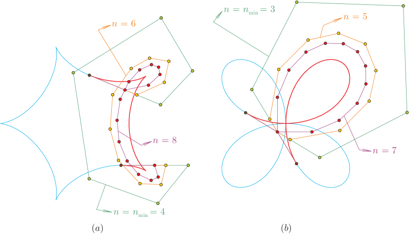
Cases (a) and (b) of Fig. 4 show the control point based exact descriptions of the hypocycloidal arc

$$\mathbf{g}\left(u\right)=\left[\begin{array}[c]{c}g^{1}\left(u\right)\\ \\ g^{2}\left(u\right)\end{array}\right]=\left[\begin{array}[c]{l}4\cos\left(u-\frac{\pi}{3}\right)+\cos\left(4u-\frac{\pi}{3}\right)\\ \\ 4\sin\left(u-\frac{\pi}{3}\right)-\sin\left(4u-\frac{\pi}{3}\right)\end{array}\right],~{}u\in\left(0,\frac{3\pi}{4}\right)$$ (44)

and of the arc

$$\mathbf{g}\left(u\right)=\left[\begin{array}[c]{c}g^{1}\left(u\right)\\ \\ g^{2}\left(u\right)\end{array}\right]=\frac{1}{2}\left[\begin{array}[c]{l}\sin\left(u-\frac{\pi}{12}\right)+\sin\left(3u-\frac{\pi}{4}\right)\\ \\ \cos\left(u-\frac{\pi}{12}\right)-\cos\left(3u-\frac{\pi}{4}\right)\end{array}\right],~{}u\in\left(0,\frac{2\pi}{3}\right)$$ (45)

of a quadrifolium, respectively.

Figure 4: Order elevated control point based exact description of trigonometric curves (44) and (45) by means of Theorem 5.1. (a) A hypocycloidal arc ($\alpha=\frac{3\pi}{4}$). (b) An arc of a quadrifolium ($\alpha=\frac{2\pi}{3}$).

Example 5.2 (Application of Theorem 5.1 – space curve)

Fig. 5 illustrates the control point based exact descriptions of the arc

$$\mathbf{g}\left(u\right)=\left[\begin{array}[c]{c}g^{1}\left(u\right)\\ \\ g^{2}\left(u\right)\\ \\ g^{3}\left(u\right)\end{array}\right]=\left[\begin{array}[c]{l}\frac{1}{2}\cos\left(u\right)+2\cos\left(3u\right)+\frac{1}{2}\cos\left(5u\right)\\ \\ \frac{1}{2}\sin\left(u\right)+2\sin\left(3u\right)+\frac{1}{2}\sin\left(5u\right)\\ \\ \sin\left(2u\right)\end{array}\right],~{}u\in\left(0,\frac{\pi}{2}\right),$$ (46)

of a torus knot.

Figure 5: Order elevated control point based exact description of an arc ($\alpha=\frac{\pi}{2}$) of a knot that lies on the surface of the torus $\left[\left(R+r\sin\left(u_{1}\right)\right)\cos\left(u_{2}\right),\left(R+r\sin\left(u_{1}\right)\right)\sin\left(u_{2}\right),r\cos\left(u_{1}\right)\right]$, where $\left(u_{1},u_{2}\right)\in\left[0,2\pi\right]\times\left[0,2\pi\right]$, $R=2$ and $r=1$. Control points were obtained by using Theorem 5.1.

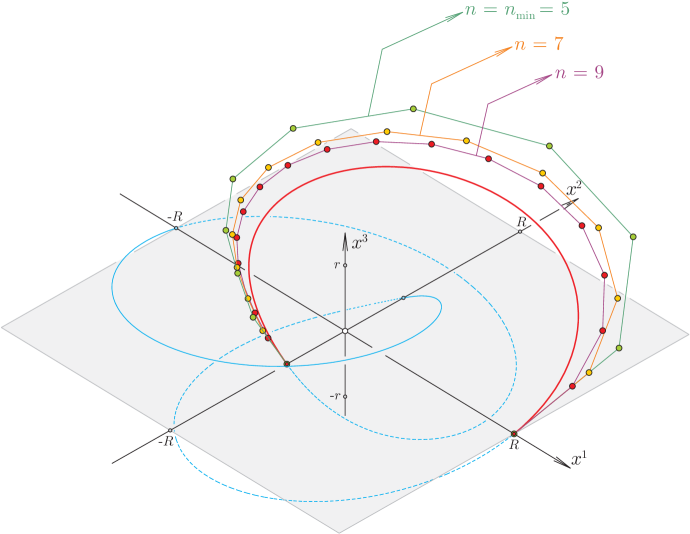
Consider now the rational trigonometric curve

$$\mathbf{g}\left(u\right)=\frac{1}{g^{\delta+1}\left(u\right)}\left[g^{\ell}\left(u\right)\right]_{\ell=1}^{\delta},~{}u\in\left[0,\alpha\right],$$ (47)

given in traditional parametric form

$$g^{\ell}\left(u\right)=\sum_{p\in P_{\ell}}c_{p}^{\ell}\cos\left(pu+\psi_{p}^{\ell}\right)+\sum_{q\in Q_{\ell}}s_{q}^{\ell}\sin\left(qu+\varphi_{q}^{\ell}\right),~{}P_{\ell},Q_{\ell}\subset\mathbb{N},~{}c_{p}^{\ell},\psi_{p}^{\ell},s_{q}^{\ell},\varphi_{q}^{\ell}\in\mathbb{R},~{}\ell=1,2,\ldots,\delta+1,$$

where

$$g^{\delta+1}\left(u\right)>0,~{}\forall u\in\left[0,\alpha\right].$$

Algorithm 5.1 (Control point based exact description of rational trigonometric curves)

The process that provides the control point based exact description of the rational curve (47) consists of the following operations:

• let

  $$n\geq n_{\min}=\max\left\{z:z\in\cup_{\ell=1}^{\delta+1}\left(P_{\ell}\cup Q_{\ell}\right)\right\}$$

  be an arbitrarily fixed order;

• apply Theorem 5.1 to the pre-image

  $$\mathbf{g}_{\wp}\left(u\right)=\left[g^{\ell}\left(u\right)\right]_{\ell=1}^{\delta+1},~{}u\in\left[0,\alpha\right]$$ (48)

  of the curve (47), i.e., compute control points

  $$\mathbf{d}_{i}^{\wp}=\left[d_{i}^{\ell}\right]_{\ell=1}^{\delta+1}\in\mathbb{R}^{\delta+1},~{}i=0,1,\ldots,2n$$

  for the exact trigonometric representation of (48) in the pre-image space $\mathbb{R}^{\delta+1}$;

• project the obtained control points onto the hyperplane $x^{\delta+1}=1$ that results the control points

  $$\mathbf{d}_{i}=\frac{1}{d_{i}^{\delta+1}}\left[d_{i}^{\ell}\right]_{\ell=1}^{\delta}\in\mathbb{R}^{\delta},~{}i=0,1,\ldots,2n$$

  and weights

  $$\omega_{i}=d_{i}^{\delta+1},~{}i=0,1,\ldots,2n$$

  needed for the rational trigonometric representation (11) of (47);

• the above generation process does not necessarily ensure the positivity of all weights, since the last coordinate of some control points in the pre-image space $\mathbb{R}^{\delta+1}$ can be negative; if this is the case, one can increase in $\mathbb{R}^{\delta+1}$ the order of the trigonometric curve used for the control point based exact description of the pre-image $\mathbf{g}_{\wp}$, since – as stated in Remark 2.4 – order elevation generates a sequence of control polygons that converges to $\mathbf{g}_{\wp}$ which is a geometric object of one branch that does not intersect the vanishing plane $x^{\delta+1}=0\,$(i.e., the $\left(\delta+1\right)$th coordinate of all its points are of the same sign); therefore, it is guaranteed that exists a finite and minimal order $n+z$ ($z\geq 1$) for which all weights are positive.

Example 5.3 (Application of Algorithm 5.1 – rational curves)

Fig. 6 shows the control point based description of an arc of the rational trigonometric curve

$$\mathbf{g}\left(u\right)=\frac{1}{g^{3}\left(u\right)}\left[\begin{array}[c]{c}g^{1}\left(u\right)\\ \\ g^{2}\left(u\right)\end{array}\right]=\frac{1}{\frac{3}{2}-\frac{1}{2}\cos\left(2u\right)}\left[\begin{array}[c]{r}\cos\left(u\right)\\ \\ \frac{1}{2}\sin\left(2u\right)\end{array}\right],~{}u\in\left[0,\frac{2\pi}{3}\right],$$ (49)

also known as Bernoulli’s lemniscate.

Figure 6: Using Algorithm 5.1 with shape parameter $\alpha=\frac{2\pi}{3}$, the left image shows the control point based exact description of an arc of Bernoulli’s lemniscate (49) by means of a fourth order rational trigonometric curve $\mathbf{g}$ (green) and its pre-image $\mathbf{g}_{\wp}$ (red). Control points $\mathbf{d}_{i}^{\wp}=\left[\begin{array}[c]{cc}\omega_{i}\mathbf{d}_{i}&\omega_{i}\end{array}\right]\in\mathbb{R}^{3}$ ($i=0,1,\ldots,8$) of the pre-image $\mathbf{g}_{\wp}=\left[g^{\ell}\left(u\right)\right]_{\ell=1}^{3}$ were obtained by the application of Theorem 5.1, while control points $\left[\mathbf{d}_{i}\right]_{i=0}^{8}$ and weights $\left[\omega_{i}\right]_{i=0}^{8}$ needed for the rational representation (11) were obtained by the central projection of points $\left[\mathbf{d}_{i}^{\wp}\right]_{i=0}^{8}$ onto the hyperplane $x^{3}=1$. The right image also illustrates the control polygons of the second and third order exact rational trigonometric representations of the same arc. (For interpretation of the references to color in this figure legend, the reader is referred to the web version of this paper.)

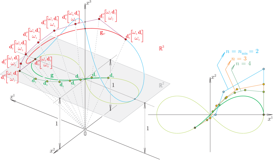
Theorem 5.1 can also be used to provide control nets (grids) for the control point based exact description of the higher order mixed partial derivatives of a general class of multivariate surfaces the elements of which can be expressed in the form

$$\mathbf{s}\left(\mathbf{u}\right)=\left[\begin{array}[c]{cccc}s^{1}\left(\mathbf{u}\right)&s^{2}\left(\mathbf{u}\right)&\cdots&s^{\delta+\kappa}\left(\mathbf{u}\right)\end{array}\right]\in\mathbb{R}^{\delta+\kappa},~{}\mathbf{u}=\left[u_{j}\right]_{j=1}^{\delta}\in\times_{j=1}^{\delta}\left[0,\alpha_{j}\right],~{}\alpha_{j}\in\left(0,\pi\right),~{}\kappa\geq 0$$ (50)

where

$$s^{\ell}\left(\mathbf{u}\right)=\sum_{\zeta=1}^{m_{\ell}}\prod_{j=1}^{\delta}\left(\sum_{p\in P_{\ell,\zeta,j}}c_{p}^{\ell,\zeta,j}\cos\left(pu_{j}+\psi_{p}^{\ell,\zeta,j}\right)+\sum_{q\in Q_{\ell,\zeta,j}}s_{q}^{\ell,\zeta,j}\sin\left(qu_{j}+\varphi_{q}^{\ell,\zeta,j}\right)\right),~{}\ell=1,2,\ldots,\delta+\kappa$$

and

$$P_{\ell,\zeta,j},Q_{\ell,\zeta,j}\subset\mathbb{N},~{}m_{\ell}\in\mathbb{N}\setminus\left\{0\right\},~{}c_{p}^{\ell,\zeta,j},\psi_{p}^{\ell,\zeta,j},s_{q}^{\ell,\zeta,j},\varphi_{q}^{\ell,\zeta,j}\in\mathbb{R}.$$

Indeed, we have the next theorem.

Theorem 5.2 (Control point based exact description of trigonometric surfaces)

The control point based exact description of the $\left(r_{1}+r_{2}+\ldots+r_{\delta}\right)$th order mixed partial derivative of the surface (50) fulfills the equality

$$\dfrac{\partial^{r_{1}+r_{2}+\ldots+r_{\delta}}}{\partial u_{1}^{r_{1}}\partial u_{2}^{r_{2}}\cdots\partial u_{\delta}^{r_{\delta}}}\mathbf{s}\left(\mathbf{u}\right)={\displaystyle\sum\limits_{i_{1}=0}^{2n_{1}}}{\displaystyle\sum\limits_{i_{2}=0}^{2n_{2}}}\cdots{\displaystyle\sum\limits_{i_{\delta}=0}^{2n_{\delta}}}\mathbf{d}_{i_{1},i_{2},\ldots,i_{\delta}}\left(r_{1},r_{2},\ldots,r_{\delta}\right){\displaystyle\prod\limits_{j=1}^{\delta}}T_{2n_{j},i_{j}}^{\alpha_{j}}\left(u_{j}\right)$$ (51)

for all parameter vectors $\mathbf{u\in}\times_{j=1}^{\delta}\left[0,\alpha_{j}\right]$, where

$$n_{j} \geq n_{\min}^{j}=\max\left\{z_{j}:z_{j}\in\cup_{\ell=1}^{\delta+k}\cup_{\zeta=1}^{m_{\ell}}\left(P_{\ell,\zeta,j}\cup Q_{\ell,\zeta,j}\right)\right\},~{}j=1,2,\ldots,\delta,$$

$$\mathbf{d}_{i_{1},i_{2},\ldots,i_{\delta}}\left(r_{1},r_{2},\ldots,r_{\delta}\right) =\left[d_{i_{1},i_{2},\ldots,i_{\delta}}^{\ell}\left(r_{1},r_{2},\ldots,r_{\delta}\right)\right]_{\ell=1}^{\delta+\kappa}\in\mathbb{R}^{\delta+\kappa},$$

$$d_{i_{1},i_{2},\ldots,i_{\delta}}^{\ell}\left(r_{1},r_{2},\ldots,r_{\delta}\right) =\sum_{\zeta=1}^{m_{\ell}}\prod_{j=1}^{\delta}d_{i_{j}}^{\ell,\zeta}\left(r_{j}\right),~{}\ell=1,2,\ldots,\delta+\kappa$$

and

$$d_{i_{j}}^{\ell,\zeta}\left(r_{j}\right)= \sum_{p\in P_{\ell,\zeta,j}}c_{p}^{\ell,\zeta,j}p^{r_{j}}\left(\mu_{p,i_{j}}^{n_{j}}\cos\left(\psi_{p}^{\ell,\zeta,j}+\frac{r_{j}\pi}{2}\right)-\lambda_{p,i_{j}}^{n_{j}}\sin\left(\psi_{p}^{\ell,\zeta,j}+\frac{r_{j}\pi}{2}\right)\right)$$

$$+\sum_{q\in Q_{\ell,\zeta,j}}s_{q}^{\ell,\zeta,j}q^{r_{j}}\left(\lambda_{q,i_{j}}^{n_{j}}\cos\left(\varphi_{q}^{\ell,\zeta,j}+\frac{r_{j}\pi}{2}\right)+\mu_{q,i_{j}}^{n_{j}}\sin\left(\varphi_{q}^{\ell,\zeta,j}+\frac{r_{j}\pi}{2}\right)\right),$$

$$\ell =1,2,\ldots,\delta+\kappa,~{}\zeta=1,2,\ldots,m_{\ell},~{}j=1,2,\ldots,\delta.$$

(In case of zeroth order partial derivatives we will use the simpler notation

$$\mathbf{d}_{i_{1},i_{2},\ldots,i_{\delta}}=\left[d_{i_{1},i_{2},\ldots,i_{\delta}}^{\ell}\right]_{\ell=1}^{\delta+\kappa}=\left[d_{i_{1},i_{2},\ldots,i_{\delta}}^{\ell}\left(0,0,\ldots,0\right)\right]_{\ell=1}^{\delta+\kappa}=\mathbf{d}_{i_{1},i_{2},\ldots,i_{\delta}}\left(0,0,\ldots,0\right)$$

for all $i_{j}=0,1,\ldots,2n_{j}$ and $j=1,2,\ldots,\delta$.)

Proof

Observe, by using Lemma 5.1, that equality

$$\frac{\partial^{r_{1}+r_{2}+\ldots+r_{\delta}}}{\partial u_{1}^{r_{1}}\partial u_{2}^{r_{2}}\cdots\partial u_{\delta}^{r_{\delta}}}s^{\ell}\left(\mathbf{u}\right)=$$

$$= \frac{\partial^{r_{1}+r_{2}+\ldots+r_{\delta}}}{\partial u_{1}^{r_{1}}\partial u_{2}^{r_{2}}\cdots\partial u_{\delta}^{r_{\delta}}}\sum_{\zeta=1}^{m_{\ell}}\prod_{j=1}^{\delta}\left(\sum_{p\in P_{\ell,\zeta,j}}c_{p}^{\ell,\zeta,j}\cos\left(pu_{j}+\psi_{p}^{\ell,\zeta,j}\right)+\sum_{q\in Q_{\ell,\zeta,j}}s_{q}^{\ell,\zeta,j}\sin\left(qu_{j}+\varphi_{q}^{\ell,\zeta,j}\right)\right)$$

$$= \sum_{\zeta=1}^{m_{\ell}}\prod_{j=1}^{\delta}\frac{\text{d}^{r_{j}}}{\text{d}u_{j}^{r_{j}}}\left(\sum_{p\in P_{\ell,\zeta,j}}c_{p}^{\ell,\zeta,j}\cos\left(pu_{j}+\psi_{p}^{\ell,\zeta,j}\right)+\sum_{q\in Q_{\ell,\zeta,j}}s_{q}^{\ell,\zeta,j}\sin\left(qu_{j}+\varphi_{q}^{\ell,\zeta,j}\right)\right)$$

$$= \sum_{\zeta=1}^{m_{\ell}}\prod_{j=1}^{\delta}\left(\sum_{i_{j}=0}^{2n_{j}}d_{i_{j}}^{\ell,\zeta}\left(r_{j}\right)T_{2n_{j},i_{j}}^{\alpha_{j}}\left(u_{j}\right)\right)$$

$$= \sum_{i_{1}=0}^{2n_{1}}\sum_{i_{2}=0}^{2n_{2}}\cdots\sum_{i_{\delta}=0}^{2n_{\delta}}\left(\sum_{\zeta=1}^{m_{\ell}}\prod_{j=1}^{\delta}d_{i_{j}}^{\ell,\zeta}\left(r_{j}\right)\right)T_{2n_{1},i_{1}}^{\alpha_{1}}\left(u_{1}\right)T_{2n_{2},i_{2}}^{\alpha_{2}}\left(u_{2}\right)\cdot\ldots\cdot T_{2n_{\delta},i_{\delta}}^{\alpha_{\delta}}\left(u_{\delta}\right)$$

holds for all parameter vectors $\mathbf{u}=\left[u_{j}\right]_{j=1}^{\delta}\in\times_{j=1}^{\delta}\left[0,\alpha_{j}\right]$ and coordinate functions $\ell=1,2,\ldots,\delta+\kappa$, i.e., $d_{i_{j}}^{\ell,\zeta}\left(r_{j}\right)$ can be calculated by means of formula (43) for all indices $\ell=1,2,\ldots,\delta+\kappa$, $\zeta=1,2,\ldots,m_{\ell}$ and $j=1,2,\ldots,\delta$.

Example 5.4 (Application of Theorem 5.2 – surfaces)

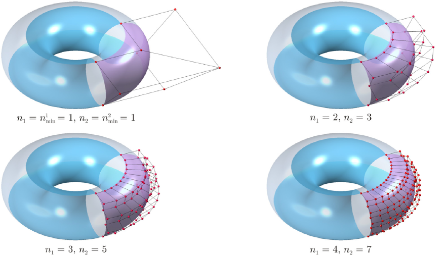
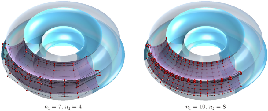
Using trigonometric surfaces of type (21) and applying Theorem 5.2, Figs. 7 and 8 show several control point constellations for the exact description of the toroidal patch

$$\mathbf{s}\left(u_{1},u_{2}\right) =\left[\begin{array}[c]{c}s^{1}\left(u_{1},u_{2}\right)\\ \\ s^{2}\left(u_{1},u_{2}\right)\\ \\ s^{3}\left(u_{1},u_{2}\right)\end{array}\right]=\left[\begin{array}[c]{c}\left(3+\frac{15}{8}\left(\sqrt{5}-1\right)\sin\left(u_{1}\right)\right)\cos\left(u_{2}\right)\\ \\ \left(3+\frac{15}{8}\left(\sqrt{5}-1\right)\sin\left(u_{1}\right)\right)\sin\left(u_{2}\right)\\ \\ \frac{15}{8}\left(\sqrt{5}-1\right)\cos\left(u_{1}\right)\end{array}\right],$$ (62)

$$\left(u_{1},u_{2}\right) \in\left[0,\frac{3\pi}{4}\right]\times\left[0,\frac{\pi}{2}\right]$$

and of the patch

$$\mathbf{s}\left(u_{1},u_{2}\right) =\left[\begin{array}[c]{c}s^{1}\left(u_{1},u_{2}\right)\\ s^{2}\left(u_{1},u_{2}\right)\\ s^{3}\left(u_{1},u_{2}\right)\end{array}\right]=\left[\begin{array}[c]{c}\left(12+6\sin\left(u_{1}\right)-\sin\left(6u_{1}\right)\right)\cos\left(u_{2}\right)\\ \left(12+6\sin\left(u_{1}\right)-\sin\left(6u_{1}\right)\right)\sin\left(u_{2}\right)\\ 6\cos\left(u_{1}\right)+\cos\left(6u_{1}\right)\end{array}\right],$$ (69)

$$\left(u_{1},u_{2}\right)\in\left[0,\frac{\pi}{2}\right]\times\left[0,\frac{2\pi}{3}\right]$$

that also lies on a surface of revolution generated by the rotation of the hypocycloid

$$\mathbf{g}\left(u\right)=\left[\begin{array}[c]{c}g^{1}\left(u\right)\\ g^{2}\left(u\right)\end{array}\right]=\left[\begin{array}[c]{c}6\sin\left(u\right)-\sin\left(6u\right)\\ 6\cos\left(u\right)+\cos\left(6u\right)\end{array}\right],~{}u\in\left[0,2\pi\right]$$ (70)

about the axis $z$, respectively.

Figure 7: Control point based exact description of the toroidal patch (62) by means of $3$-dimensional $2$-variate trigonometric surfaces of the type (21). Control nets corresponding to different orders were obtained by using Theorem 5.2 with parameter settings $\delta=2$, $\kappa=1$; $\alpha_{1}=\frac{3\pi}{4}$, $\alpha_{2}=\frac{\pi}{2}$; $m_{1}=m_{2}=m_{3}=1$; $P_{1,1,1}=\left\{0\right\}$, $P_{1,1,2}=\left\{1\right\}$, $Q_{1,1,1}=\left\{1\right\}$, $Q_{1,1,2}=\varnothing$, $c_{0}^{1,1,1}=3$, $c_{1}^{1,1,2}=1$, $s_{1}^{1,1,1}=\frac{15}{8}\left(\sqrt{5}-1\right)$, $\psi_{0}^{1,1,1}=\psi_{1}^{1,1,2}=\varphi_{1}^{1,1,1}=0$; $P_{2,1,1}=\left\{0\right\}$, $P_{2,1,2}=\varnothing$, $Q_{2,1,1}=Q_{2,1,2}=\left\{1\right\}$, $c_{0}^{2,1,1}=3$, $s_{1}^{2,1,1}=\frac{15}{8}\left(\sqrt{5}-1\right)$, $s_{1}^{2,1,2}=1$, $\psi_{0}^{2,1,1}=\varphi_{1}^{2,1,1}=\varphi_{1}^{2,1,2}=0$; $P_{3,1,1}=\left\{1\right\}$, $P_{3,1,2}=\left\{0\right\}$, $Q_{3,1,1}=Q_{3,1,2}=\varnothing$, $c_{1}^{3,1,1}=\frac{15}{8}\left(\sqrt{5}-1\right)$, $c_{0}^{3,1,2}=1$, $\psi_{0}^{3,1,1}=\psi_{1}^{3,1,2}=0$.

Figure 8: Control point based exact description of the trigonometric patch (69) that lies on a surface of revolution generated by the rotation of the hypocycloid (70) about the axis $z$. Control nets were generated by formulae described in Theorem 5.2 ($\delta=2$, $\kappa=1$; $\alpha_{1}=\frac{\pi}{2}$, $\alpha_{2}=\frac{2\pi}{3}$; $m_{1}=m_{2}=m_{3}=1$).

Example 5.5 (Application of Theorem 5.2 – volumes)

$3$-dimensional trigonometric volumes can also be exactly described by means of $3$-variate tensor product surfaces of the type (21). Figs. 9 and 10 illustrate control grids that generate the volumes

$$\mathbf{s}\left(u_{1},u_{2},u_{3}\right) =\left[\begin{array}[c]{c}s^{1}\left(u_{1},u_{2},u_{3}\right)\\ s^{2}\left(u_{1},u_{2},u_{3}\right)\\ s^{3}\left(u_{1},u_{2},u_{3}\right)\end{array}\right]$$ (74)

$$=\left[\begin{array}[c]{c}\left(6+\cos\left(u_{1}+\frac{\pi}{3}\right)\right)\cos\left(u_{2}-\frac{\pi}{6}\right)\cos\left(u_{3}+\frac{\pi}{3}\right)\\ \\ \left(6+\cos\left(u_{1}+\frac{\pi}{3}\right)\right)\cos\left(u_{2}-\frac{\pi}{6}\right)\sin\left(u_{3}+\frac{\pi}{3}\right)\\ \\ \cos\left(u_{1}+\frac{\pi}{3}\right)\sin\left(u_{2}-\frac{\pi}{6}\right)\end{array}\right],$$ (80)

$$\left(u_{1},u_{2},u_{3}\right) \in\left[0,\frac{\pi}{2}\right]\times\left[0,\frac{\pi}{2}\right]\times\left[0,\frac{2\pi}{3}\right]$$

and

$$\mathbf{s}\left(u_{1},u_{2},u_{3}\right) =\left[\begin{array}[c]{c}s^{1}\left(u_{1},u_{2},u_{3}\right)\\ s^{2}\left(u_{1},u_{2},u_{3}\right)\\ s^{3}\left(u_{1},u_{2},u_{3}\right)\end{array}\right]$$ (84)

$$=\left[\begin{array}[c]{c}\left(2+\frac{3}{4}\sin\left(u_{1}\right)-\frac{1}{4}\sin\left(3u_{1}\right)\right)\cos\left(u_{2}\right)\left(\frac{3}{2}-\frac{1}{2}\cos\left(2u_{3}\right)\right)\\ \\ \left(\frac{5}{2}-\frac{1}{2}\cos\left(2u_{1}\right)\right)\sin\left(u_{2}\right)\left(1+\frac{3}{4}\sin\left(u_{3}\right)-\frac{1}{4}\sin\left(3u_{3}\right)\right)\\ \\ \left(\frac{1}{2}+\frac{3}{8}\cos\left(u_{1}\right)+\frac{1}{2}\cos\left(2u_{1}\right)+\frac{1}{8}\cos\left(3u_{1}\right)\right)\left(\frac{3}{2}+\cos\left(u_{2}\right)+\sin\left(u_{3}\right)\right)\end{array}\right],$$ (90)

$$\left(u_{1},u_{2},u_{3}\right) \in\left[0,\frac{\pi}{2}\right]\times\left[0,\frac{2\pi}{3}\right]\times\left[0,\frac{\pi}{2}\right],$$

respectively.

Figure 9: Different views of the same $3$-dimensional trigonometric volume (80) along with its control grid calculated by means of Theorem 5.2 ($\delta=3$, $\kappa=0$; $\alpha_{1}=\frac{\pi}{2}$, $\alpha_{2}=\frac{\pi}{2}$, $\alpha_{3}=\frac{2\pi}{3}$; $m_{1}=m_{2}=m_{3}=1$).

Figure 10: Control point based exact description of the $3$-dimensional trigonometric volume (90) by means of $3$-variate tensor product surfaces of the type (21) with different orders. Control grids were obtained by using Theorem 5.2 ($\delta=3$, $\kappa=0$; $\alpha_{1}=\frac{\pi}{2}$, $\alpha_{2}=\frac{2\pi}{3}$, $\alpha_{3}=\frac{\pi}{2}$; $m_{1}=m_{2}=1$, $m_{3}=2$).

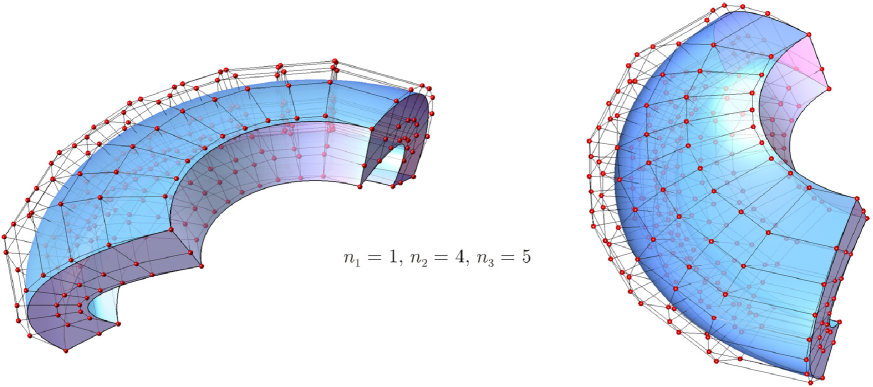
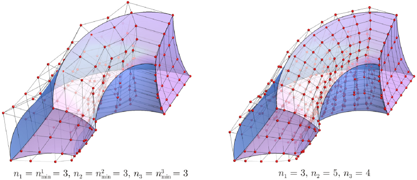
Theorem 5.2 can also be used to provide control point based exact description of the rational trigonometric surface

$$\mathbf{s}\left(\mathbf{u}\right)=\frac{1}{s^{\delta+\kappa+1}\left(\mathbf{u}\right)}\left[\begin{array}[c]{cccc}s^{1}\left(\mathbf{u}\right)&s^{2}\left(\mathbf{u}\right)&\cdots&s^{\delta+\kappa}\left(\mathbf{u}\right)\end{array}\right]\in\mathbb{R}^{\delta+\kappa},$$ (91)

where

$$\mathbf{u} =\left[u_{j}\right]_{j=1}^{\delta}\in\times_{j=1}^{\delta}\left[0,\alpha_{j}\right],~{}\alpha_{j}\in\left(0,\pi\right),~{}\kappa\geq 0,$$

$$s^{\ell}\left(\mathbf{u}\right) =\sum_{\zeta=1}^{m_{\ell}}\prod_{j=1}^{\delta}\left(\sum_{p\in P_{\ell,\zeta,j}}c_{p}^{\ell,\zeta,j}\cos\left(pu_{j}+\psi_{p}^{\ell,\zeta,j}\right)+\sum_{q\in Q_{\ell,\zeta,j}}s_{q}^{\ell,\zeta,j}\sin\left(qu_{j}+\varphi_{q}^{\ell,\zeta,j}\right)\right),$$

$$\ell =1,2,\ldots,\delta+\kappa+1,$$

$$P_{\ell,\zeta,j},Q_{\ell,\zeta,j} \subset\mathbb{N},~{}m_{\ell}\in\mathbb{N}\setminus\left\{0\right\},~{}c_{p}^{\ell,\zeta,j},\psi_{p}^{\ell,\zeta,j},s_{q}^{\ell,\zeta,j},\varphi_{q}^{\ell,\zeta,j}\in\mathbb{R}$$

and

$$s^{\delta+\kappa+1}\left(\mathbf{u}\right)>0,~{}\forall\mathbf{u}\in\times_{j=1}^{\delta}\left[0,\alpha_{j}\right].$$

Similarly to Algorithm 5.1 one can formulate the next process.

Algorithm 5.2 (Control point based exact description of rational trigonometric surfaces)

Operations that ensure the control point based exact description of the surface (91) are as follows:

• let

  $$n_{j}\geq n_{\min}^{j}=\max\left\{z_{j}:z_{j}\in\cup_{\ell=1}^{\delta+\kappa+1}\cup_{\zeta=1}^{m_{\ell}}\left(P_{\ell,\zeta,j}\cup Q_{\ell,\zeta,j}\right)\right\},~{}j=1,2,\ldots,\delta$$

  be arbitrarily fixed orders in directions $u_{1},u_{2},\ldots,u_{\delta}$;

• apply Theorem 5.2 to the pre-image

  $$\mathbf{s}_{\wp}\left(\mathbf{u}\right)=\left[s^{\ell}\left(\mathbf{u}\right)\right]_{\ell=1}^{\delta+\kappa+1}\in\mathbb{R}^{\delta+\kappa+1},~{}\mathbf{u}=\left[u_{j}\right]_{j=1}^{\delta}\in\times_{j=1}^{\delta}\left[0,\alpha_{j}\right]$$ (92)

  of the surface (91), i.e., compute control points

  $$\mathbf{d}_{i_{1},i_{2},\ldots,i_{\delta}}^{\wp}=\left[d_{i_{1},i_{2},\ldots,i_{\delta}}^{\ell}\right]_{\ell=1}^{\delta+\kappa+1}\in\mathbb{R}^{\delta+\kappa+1},~{}i_{j}=0,1,\ldots,2n_{j},~{}j=1,2,\ldots,\delta$$

  for the exact trigonometric representation of (92) in the pre-image space $\mathbb{R}^{\delta+\kappa+1}$;

• project the obtained control points onto the hyperplane $x^{\delta+\kappa+1}=1$ that results the control points

  $$\mathbf{d}_{i_{1},i_{2},\ldots,i_{\delta}}=\frac{1}{d_{i_{1},i_{2},\ldots,i_{\delta}}^{\delta+\kappa+1}}\left[d_{i_{1},i_{2},\ldots,i_{\delta}}^{\ell}\right]_{\ell=1}^{\delta+\kappa}\in\mathbb{R}^{\delta+\kappa},~{}i_{j}=0,1,\ldots,2n_{j},~{}j=1,2,\ldots,\delta$$

  and weights

  $$\omega_{i_{1},i_{2},\ldots,i_{\delta}}=d_{i_{1},i_{2},\ldots,i_{\delta}}^{\delta+\kappa+1},~{}i_{j}=0,1,\ldots,2n_{j},~{}j=1,2,\ldots,\delta$$

  needed for the rational trigonometric representation (23) of (91);

• if not all weights are positive, try to increase the components of the order $\left(n_{1},n_{2},\ldots,n_{\delta}\right)$ of the trigonometric surface used for the control point based exact description of the pre-image $\mathbf{s}_{\wp}$ in $\mathbb{R}^{\delta+\kappa+1}$ and repeat the previous projectional and weight determination step.

Example 5.6 (Application of Algorithm 5.2 – rational surfaces)

Using surfaces of the type (23), Fig. 11 shows the control point based exact description of the rational trigonometric patch

$$\mathbf{s}\left(u_{1},u_{2}\right)=\frac{1}{s^{4}\left(u_{1},u_{2}-\gamma\right)}\left[\begin{array}[c]{c}s^{1}\left(u_{1},u_{2}-\gamma\right)\\ s^{2}\left(u_{1},u_{2}-\gamma\right)\\ s^{3}\left(u_{1},u_{2}-\gamma\right)\end{array}\right],~{}\left(u_{1},u_{2}\right)\in\left[0,\frac{\pi}{4}\right]\times\left[0,\frac{\pi}{3}\right],$$ (93)

where

$$s^{1}\left(u_{1},u_{2}\right)= \cos\left(u_{1}\right)\left(173\cos\left(u_{2}\right)-10\sin\left(3u_{2}\right)-10\sin\left(5u_{2}\right)+\cos\left(7u_{2}\right)+\cos\left(9u_{2}\right)\right)$$

$$+\sin\left(u_{1}\right)\left(-173\sin\left(u_{2}\right)+10\cos\left(3u_{2}\right)-10\cos\left(5u_{2}\right)+\sin\left(7u_{2}\right)-\sin\left(9u_{2}\right)\right),$$

$$s^{2}\left(u_{1},u_{2}\right)= \cos\left(u_{1}\right)\left(173\sin\left(u_{2}\right)-10\cos\left(3u_{2}\right)+10\cos\left(5u_{2}\right)-\sin\left(7u_{2}\right)+\sin\left(9u_{2}\right)\right)$$

$$+\sin\left(u_{1}\right)\left(173\cos\left(u_{2}\right)-10\sin\left(3u_{2}\right)-10\sin\left(5u_{2}\right)+\cos\left(7u_{2}\right)+\cos\left(9u_{2}\right)\right),$$

$$s^{3}\left(u_{1},u_{2}\right)= 20\cos\left(u_{1}\right)\left(5\cos\left(u_{2}\right)+\sin\left(3u_{2}\right)+\sin\left(5u_{2}\right)\right)$$

$$+20\sin\left(u_{1}\right)\left(5\sin\left(u_{2}\right)+\cos\left(3u_{2}\right)-\cos\left(5u_{2}\right)\right),$$

$$s^{4}\left(u_{1},u_{2}\right)= 20\cos\left(u_{1}\right)\left(5\sin\left(u_{2}\right)+\cos\left(3u_{2}\right)-\cos\left(5u_{2}\right)\right)$$

$$-20\sin\left(u_{1}\right)\left(5\cos\left(u_{2}\right)+\sin\left(3u_{2}\right)+\sin\left(5u_{2}\right)\right)+200$$

and $\gamma=\frac{\pi}{3}$.

Figure 11: Control point based exact description of the patch (93) by means of $3$-dimensional $2$-variate rational trigonometric patches of different orders. Control nets were obtained by following the steps of Algorithm 5.2 ($\delta=2$, $\kappa=1$; $\alpha_{1}=\frac{\pi}{4}$, $\alpha_{2}=\frac{\pi}{3}$; $m_{1}=m_{2}=m_{3}=2$, $m_{4}=3$).

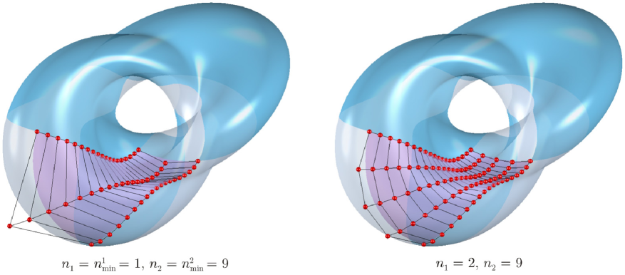
5.2 Description of (rational) hyperbolic curves and surfaces

Assume that the smooth parametric curve

$$\mathbf{g}\left(u\right)=\left[g^{\ell}\left(u\right)\right]_{\ell=1}^{\delta},~{}u\in\left[0,\alpha\right],~{}\alpha>0$$ (94)

has coordinate functions of the form

$$g^{\ell}\left(u\right)=\sum_{p\in P_{\ell}}c_{p}^{\ell}\cosh\left(pu+\psi_{p}^{\ell}\right)+\sum_{q\in Q_{\ell}}s_{q}^{\ell}\sinh\left(qu+\varphi_{q}^{\ell}\right),$$

where $P_{\ell},Q_{\ell}\subset\mathbb{N}$ and $c_{p}^{\ell},\psi_{p}^{\ell},s_{q}^{\ell},\varphi_{q}^{\ell}\in\mathbb{R}$ and consider the vector space (2) of order

$$n\geq n_{\min}=\max\left\{z:z\in\cup_{\ell=1}^{\delta}\left(P_{\ell}\cup Q_{\ell}\right)\right\}.$$ (95)

Using Lemma 5.2 and performing calculations similar to the proof of Theorem 5.1 one obtains the next statement.

Theorem 5.3 (Control point based exact description of hyperbolic curves)

For any arbitrarily fixed order (95) the curve (94) given in traditional hyperbolic parametric form has a unique control point based exact description, more precisely one has that

$$\frac{\text{\emph{d}}^{r}}{\text{\emph{d}}u^{r}}g^{\ell}\left(u\right)=\sum_{i=0}^{2n}d_{i}^{\ell}\left(r\right)H_{2n,i}^{\alpha}\left(u\right),$$

where

$$d_{i}^{\ell}\left(r\right)=\left\{\begin{array}[c]{ll}{\displaystyle\sum\limits_{p\in P_{\ell}}}c_{p}^{\ell}p^{r}\left(\rho_{p,i}^{n}\cosh\left(\psi_{p}^{\ell}\right)+\sigma_{p,i}^{n}\sinh\left(\psi_{p}^{\ell}\right)\right)&\\ +{\displaystyle\sum\limits_{q\in Q_{\ell}}}s_{q}^{\ell}q^{r}\left(\sigma_{q,i}^{n}\cosh\left(\varphi_{q}^{\ell}\right)+\rho_{q,i}^{n}\sinh\left(\varphi_{q}^{\ell}\right)\right),&r=2z,\\ &\\ {\displaystyle\sum\limits_{p\in P_{\ell}}}c_{p}^{\ell}p^{r}\left(\sigma_{p,i}^{n}\cosh\left(\psi_{p}^{\ell}\right)+\rho_{p,i}^{n}\sinh\left(\psi_{p}^{\ell}\right)\right)&\\ +{\displaystyle\sum\limits_{q\in Q_{\ell}}}s_{q}^{\ell}q^{r}\left(\rho_{q,i}^{n}\cosh\left(\varphi_{q}^{\ell}\right)+\sigma_{q,i}^{n}\sinh\left(\varphi_{q}^{\ell}\right)\right),&r=2z+1\end{array}\right.$$

denotes the $\ell$th coordinate of the $i$th control point $\mathbf{d}_{i}$ needed for the hyperbolic curve description (15).

Example 5.7 (Application of Theorem 5.3 – curves)

Fig. 12 shows the control point based description of the arc

$$\mathbf{g}\left(u\right)=\left[\begin{array}[c]{c}g^{1}\left(u\right)\\ \\ g^{2}\left(u\right)\end{array}\right]=\left[\begin{array}[c]{r}\sinh\left(u-\frac{3}{2}\right)\\ \\ \cosh\left(u-\frac{3}{2}\right)\end{array}\right],~{}u\in\left[0,3\right]$$ (96)

of an equilateral hyperbola.

Figure 12: Using Theorem 5.3, the image shows the control point based exact description of the hyperbolic arc (96) by means of hyperbolic curves of the type (15) of varying order and fixed shape parameter $\alpha=3$.

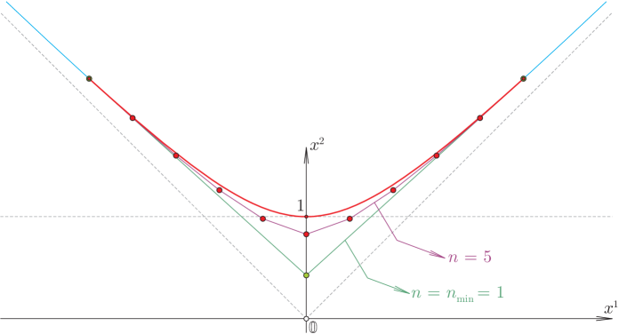
Remark 5.11 (Hyperbolic counterpart of Theorem 5.2)

Higher order (mixed) partial derivatives of a non-rational higher dimensional multivariate hyperbolic surface can also be exactly described by means of Theorem 5.3; one would simply obtain the hyperbolic counterpart of Theorem 5.2. Moreover, one can combine Theorems 5.1 and 5.3 in order to exactly describe patches of hybrid multivariate surfaces

$$\mathbf{s}\left(\mathbf{u}\right)=\left[\begin{array}[c]{cccc}s^{1}\left(\mathbf{u}\right)&s^{2}\left(\mathbf{u}\right)&\cdots&s^{\delta+\kappa}\left(\mathbf{u}\right)\end{array}\right]\in\mathbb{R}^{\delta+\kappa},~{}\mathbf{u}=\left[u_{j}\right]_{j=1}^{\delta}\in\times_{j=1}^{\delta}\left[0,\alpha_{j}\right],~{}\alpha_{j}\in\left(0,\beta_{j}\right),~{}\kappa\geq 0$$

that are either trigonometric or hyperbolic in case of a fixed direction $u_{j}$, where $\beta_{j}$ is either $\pi$ or $+\infty$ depending on the trigonometric or hyperbolic type of the coordinate function $s^{j}$, respectively. (Along a selected direction each coordinate function must be of the same type).

Example 5.8 (Combination of Theorems 5.1 and 5.3  – hybrid surfaces)

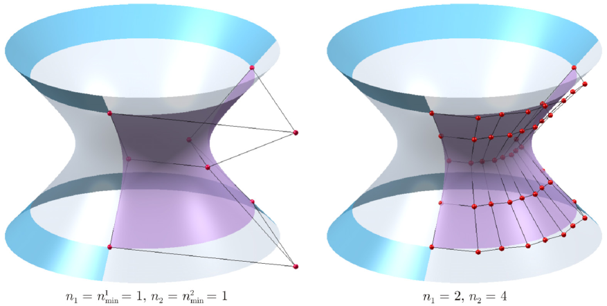
Fig. 13 illustrates the control point based exact description of the patch

$$\mathbf{s}\left(u_{1},u_{2}\right)=\left[\begin{array}[c]{c}s^{1}\left(u_{1},u_{2}\right)\\ \\ s^{2}\left(u_{1},u_{2}\right)\\ \\ s^{3}\left(u_{1},u_{2}\right)\end{array}\right]=\left[\begin{array}[c]{c}\left(1+\cosh\left(u_{1}-\frac{3}{2}\right)\right)\sin\left(u_{2}\right)\\ \\ \left(1+\cosh\left(u_{1}-\frac{3}{2}\right)\right)\cos\left(u_{2}\right)\\ \\ \sinh\left(u_{1}-\frac{3}{2}\right)\end{array}\right],~{}\left(u_{1},u_{2}\right)\in\left[0,3\right]\times\left[0,\frac{2\pi}{3}\right]$$ (97)

that lies on a surface of revolution (also called hyperboloid) obtained by the rotation of the equilateral hyperbolic arc

$$\mathbf{g}\left(u\right)=\left[\begin{array}[c]{c}g^{1}\left(u\right)\\ \\ g^{2}\left(u\right)\end{array}\right]=\left[\begin{array}[c]{r}\cosh\left(u-\frac{3}{2}\right)\\ \\ \sinh\left(u-\frac{3}{2}\right)\end{array}\right],~{}u\in\left[0,3\right]$$ (98)

along the axis $z$.

Figure 13: Control point based exact description of the hyperboloidal patch (97) with hybrid surfaces of different orders. In order to formulate the hybrid variant of Theorem 5.2, in directions $u_{1}$ and $u_{2}$ the results of Theorems 5.3 ($\alpha_{1}=3$) and 5.1 ($\alpha_{2}=\frac{2\pi}{3}$) were applied ($m_{1}=m_{2}=m_{3}=1$), respectively.

Remark 5.12 (Hyperbolic counterpart of Algorithms 5.1 and 5.2)

Any smooth rational hyperbolic curve/surface that is given in traditional parametric form (with a non-vanishing function in its denominator) can also be exactly described by means of rational hyperbolic curves/surfaces of the type (18)/(29); one simply has to apply the hyperbolic counterpart of Algorithms 5.1 or 5.2. Moreover, combining the presented trigonometric algorithms and their hyperbolic counterparts, higher dimensional hybrid multivariate rational surfaces can also exactly described by means of multivariate hybrid tensor product surfaces.

Example 5.9 (Applying the hyperbolic counterpart of Algorithm 5.1 )

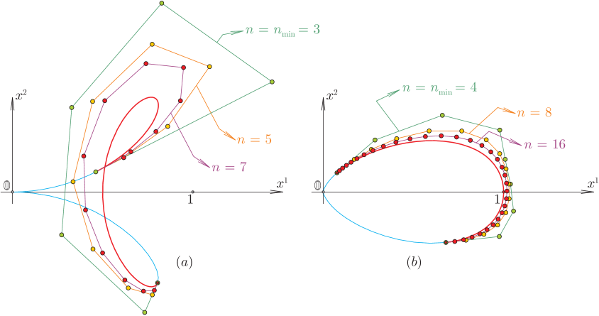
Cases (a) and (b) of Fig. 14 show the control point based exact description of the rational hyperbolic arcs

$$\mathbf{g}\left(u\right)=\frac{1}{g^{3}\left(u\right)}\left[\begin{array}[c]{c}g^{1}\left(u\right)\\ g^{2}\left(u\right)\end{array}\right]=\frac{1}{4+3\cosh\left(u-1\right)+\cosh\left(3u-3\right)}\left[\begin{array}[c]{r}4\cosh\left(2u-2\right)\\ 8\sinh\left(u-1\right)\end{array}\right],~{}u\in\left[0,3.1\right]$$ (99)

and

$$\mathbf{g}\left(u\right)=\frac{1}{g^{3}\left(u\right)}\left[\begin{array}[c]{c}g^{1}\left(u\right)\\ \\ g^{2}\left(u\right)\end{array}\right]=\frac{1}{11+4\cosh\left(2u-\frac{3}{2}\right)+\cosh\left(4u-3\right)}\left[\begin{array}[c]{c}16\cosh\left(u-\frac{3}{4}\right)\\ \\ 4\sinh\left(2u-\frac{3}{2}\right)\end{array}\right],~{}u\in\left[0,2.5\right]$$ (100)

respectively. (Note that in both cases $\lim\limits_{u\rightarrow\pm\infty}\mathbf{g}\left(u\right)=\mathbf{0}$.)

Figure 14: Using rational hyperbolic curves of the type (18), cases (a) and (b) illustrate the control point based exact description of arcs (99) and (100), respectively. Control polygons were determined by the hyperbolic counterpart of Algorithm 5.1.

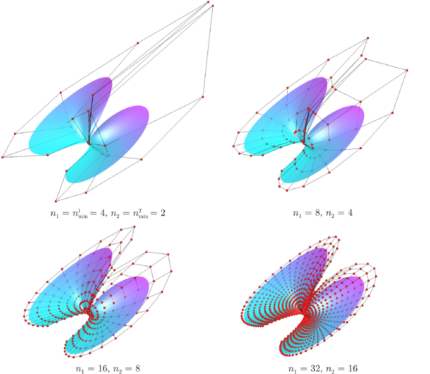
Example 5.10 (Applying the hyperbolic counterpart of Algorithm 5.2)

Using surfaces of the type (29), Fig. 15 illustrates several control point configurations for the exact description of the rational hyperbolic surface patch

$$\mathbf{s}\left(u_{1},u_{2}\right)=\frac{1}{s^{4}\left(u_{1},u_{2}\right)}\left[\begin{array}[c]{c}s^{1}\left(u_{1},u_{2}\right)\\ s^{2}\left(u_{1},u_{2}\right)\\ s^{3}\left(u_{1},u_{2}\right)\end{array}\right],~{}\left(u_{1},u_{2}\right)\in\left[0,6\right]\times\left[0,10\right],$$ (101)

where

$$s^{1}\left(u_{1},u_{2}\right) =6\left(\cosh\left(2u_{1}-2\right)+\sinh\left(u_{2}-5\right)\right),$$

$$s^{2}\left(u_{1},u_{2}\right) =\frac{1}{10}\sinh\left(u_{1}-1\right)\cosh\left(2u_{2}-10\right),$$

$$s^{3}\left(u_{1},u_{2}\right) =2\left(\sinh\left(2u_{1}-2\right)+\cosh\left(2u_{1}-2\right)\right)\cosh\left(u_{2}-5\right),$$

$$s^{4}\left(u_{1},u_{2}\right) =275+100\cosh(2u_{1}-2)+25\cosh(4u_{1}-4).$$

Figure 15: Control point based exact description of the patch (101) by means of rational hyperbolic surfaces of the type (29). Control nets were obtained by the hyperbolic counterpart of Algorithm 5.2 ($\delta=2$, $\kappa=1$; $\alpha_{1}=6$, $\alpha_{2}=10$; $m_{1}=2$, $m_{2}=m_{3}=m_{4}=1$).

Example 5.11 (Hybrid counterpart of Algorithm 5.2 – hybrid rational volumes)

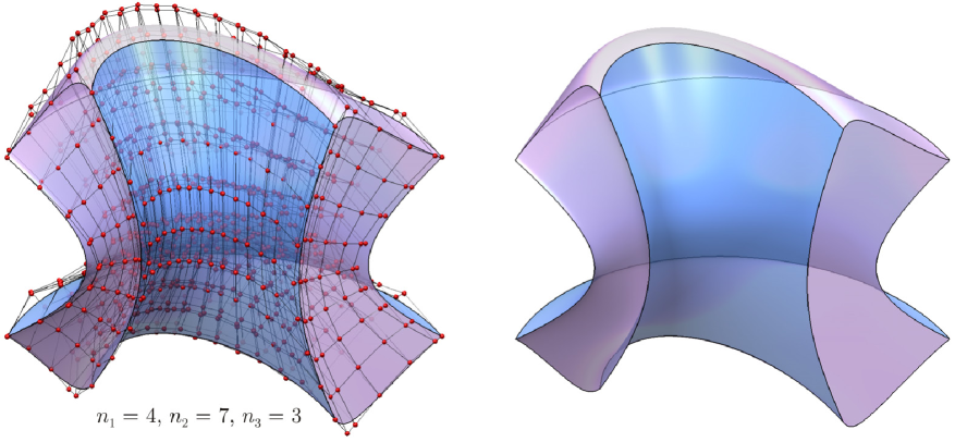
Using multivariate rational tensor product surfaces specified by functions that are exclusively either trigonometric or hyperbolic in each of their variables, Fig. 16 shows the control point based exact description of the $3$-dimensional $3$-variate rational surface element (volume)

$$\mathbf{s}\left(\mathbf{u}\right)=\frac{1}{s^{4}\left(u_{1},u_{2},u_{3}\right)}\left[\begin{array}[c]{c}s^{1}\left(u_{1},u_{2},u_{3}\right)\\ s^{2}\left(u_{1},u_{2},u_{3}\right)\\ s^{3}\left(u_{1},u_{2},u_{3}\right)\end{array}\right],~{}\left(u_{1},u_{2},u_{3}\right)\in\left[0,2\right]\times\left[0,\frac{3\pi}{4}\right]\times\left[0,\frac{\pi}{2}\right]$$ (102)

where functions

$$s^{1}\left(u_{1},u_{2},u_{3}\right)= \frac{5}{4}\cosh\left(u_{1}-1\right)\cos\left(u_{2}\right)\left(\frac{3}{2}+\frac{3}{4}\sin\left(u_{3}\right)-\frac{1}{2}\cos\left(u_{3}\right)-\frac{1}{4}\sin\left(3u_{3}\right)\right),$$

$$s^{2}\left(u_{1},u_{2},u_{3}\right)= \cosh\left(u_{1}-1\right)\sin\left(u_{2}\right)\left(\frac{5}{2}+\frac{3}{4}\sin\left(u_{3}\right)-\frac{1}{4}\sin\left(3u_{3}\right)\right),$$

$$s^{3}\left(u_{1},u_{2},u_{3}\right)= -\frac{5}{4}\sinh\left(u_{1}-1\right)\left(\frac{7}{4}+\frac{1}{4}\cos\left(2u_{3}\right)\right),$$

$$s^{4}\left(u_{1},u_{2},u_{3}\right)= 1-\frac{3}{32}\sqrt{2-\sqrt{2}}\sin\left(u_{3}\right)-\frac{3}{32}\sqrt{2+\sqrt{2}}\cos\left(u_{3}\right)-\frac{1}{32}\sqrt{2+\sqrt{2}}\sin\left(3u_{3}\right)-\frac{1}{32}\sqrt{2-\sqrt{2}}\cos\left(3u_{3}\right)$$

are hyperbolic or trigonometric in the first and the last two variables, respectively.

Figure 16: Control point based exact description of the hybrid $3$-dimensional rational volume element (102). The control grid was calculated by using the hybrid counterpart of Algorithm 5.2 ($\delta=3$, $\kappa=0$; $\alpha_{1}=2$, $\alpha_{2}=\frac{3\pi}{4}$, $\alpha_{3}=\frac{\pi}{2}$; $m_{1}=m_{2}=m_{3}=m_{4}=1$).

6 Final remarks

Subdivision algorithms of trigonometric and hyperbolic curves detailed in Section 2 can also be easily extended to higher dimensional multivariate (rational) trigonometric or hyperbolic surfaces, respectively. Therefore, similarly to standard rational Bézier curves and surfaces that are present in the core of major CAD/CAM systems, all subdivision based important curve and surface design algorithms (like evaluation or intersection detection) can be both mathematically and programmatically treated in a unified way by means of normalized B-bases (5) and (13). Considering the large variety of (rational) curves and multivariate surfaces that can be exactly described by means of control points and the fact that classical (rational) Bézier curves and multivariate surfaces are special limiting cases of the corresponding curve and surface modeling tools defined in Sections 2 and 3, it is worthwhile to incorporate all proposed techniques and algorithms presented in Section 5 into CAD systems of our days.