A 2.5% measurement of the growth rate from small-scale redshift space clustering of SDSS-III CMASS galaxies
Abstract
We perform the first fit to the anisotropic clustering of SDSS-III CMASS DR10 galaxies on scales of Mpc. A standard halo occupation distribution model evaluated near the best fit Planck CDM cosmology provides a good fit to the observed anisotropic clustering, and implies a normalization for the peculiar velocity field of halos of . Since this constraint includes both quasi-linear and non-linear scales, it should severely constrain modified gravity models that enhance pairwise infall velocities on these scales. Though model dependent, our measurement represents a factor of 2.5 improvement in precision over the analysis of DR11 on large scales, , and is the tightest single constraint on the growth rate of cosmic structure to date. Our measurement is consistent with the Planck CDM prediction of at the level. Assuming a halo mass function evaluated at the best fit Planck cosmology, we also find that of CMASS galaxies are satellites in halos of mass . While none of our tests and model generalizations indicate systematic errors due to an insufficiently detailed model of the galaxy-halo connection, the precision of these first results warrant further investigation into the modeling uncertainties and degeneracies with cosmological parameters.
keywords:
cosmology: large-scale structure of Universe, cosmological parameters, galaxies: haloes, statistics1 Introduction
The clustering of galaxies on small scales provides important constraints on the relationship between galaxies and the underlying dark matter distribution. This relation is of interest in itself as a constraint on galaxy formation and evolution, as well as for quantifying the impact of galaxy-formation scale physics on larger scale clustering measures used for cosmological parameter constraints. Modern approaches to modeling the relationship between galaxies and the underlying dark matter distribution rely on the basic tenet that galaxy formation requires a gravitationally-bound dark matter halo or sub-halo to accumulate and condense gas (Peacock & Smith, 2000; Seljak, 2000; Benson et al., 2000; White, Hernquist, & Springel, 2001; Berlind & Weinberg, 2002; Cooray & Sheth, 2002; Yang, Mo, & van den Bosch, 2003). In their simplest form, such “halo models” contain one dominant variable that determines the probability that a (sub-)halo hosts a galaxy of interest. In the halo occupation distribution (HOD) formalism adopted in this paper, halo mass is the dominant variable and halos are permitted to host more than one galaxy. In the sub-halo abundance matching (“SHAM”) formalism, the maximum circular velocity at accretion is often used (Marinoni & Hudson, 2002; Vale & Ostriker, 2006; Conroy, Wechsler, & Kravtsov, 2006). The primary advantage of SHAM is that each sub-halo hosts only a single galaxy, thus requiring fewer free parameters to specify the model but assuming a specific but physically motivated relation between central and satellite galaxies. The practical disadvantage is that -body simulations require higher resolution to resolve sub-halos. In principle both of these approaches could be generalized to include additional secondary variables such as halo formation time, with observable consequences (Gao et al., 2005; Wang et al., 2013; Zentner, Hearin, van den Bosch, 2013; Cohn & White, 2013).
There are a host of observables available to constrain halo models as a function of galaxy properties: one-point statistics like number density or luminosity functions, two- or three-point galaxy clustering (Zehavi et al., 2011; Marin, 2011), marked statistics (Sheth, 2005; White & Padmanabhan, 2009) and direct measurements the galaxy group multiplicity function (Yang, Mo, & van den Bosch, 2009; Reid & Spergel, 2009). The most widely used observable is the projected correlation function, , which removes sensitivity to redshift space distortions by integrating over the line-of-sight separation. While redshift space distortion effects are more difficult to model, they do provide complementary constraints both on the velocity distribution of galaxies relative to their host dark matter halos (van den Bosch et al., 2005) and on cosmological parameters (Yang et al., 2004).
The primary goal of the present paper is to use the information in the anisotropy of the galaxy correlation function on scales Mpc to simultaneously constrain the HOD and growth rate of cosmic structure through the pairwise infall of galaxies caused by their mutual gravitational attraction (Kaiser, 1987). Constraints on gravitational infall on these scales is of particular interest in searching for signatures of modified gravity: for instance, an model with predicts a increase in the amplitude of pairwise infall velocities on scales of 10-30 Mpc (Keisler, 2013; Zu et al., 2013; Lam et al., 2012). Alternatively, the non-linear regime is also a promising avenue for constraining dark sector coupling (Piloyan et al., 2014). We can also use the constraints on the HOD to infer the nuisance parameter employed in our analysis on larger scales (Reid et al., 2012; Samushia et al., 2013) to account for the velocity dispersions of galaxies relative to their host dark matter halos. See Hikage (2014) for a similar concept applied to the power spectrum multipoles.
In this paper we focus on the CMASS sample from the SDSS-III Baryon Oscillation Spectroscopic Survey (BOSS). This sample has thus far been the focus of several cosmological analyses, most recently providing a one per-cent absolute distance measurement using the baryon acoustic oscillation (BAO) standard ruler (Anderson et al., 2013) and a 6% constraint on the growth rate of cosmic structure (Samushia et al., 2013; Beutler et al., 2013; Sanchez et al., 2013; Chuang et al., 2013). The projected correlation function of these galaxies has also been used to constrain halo models using both the HOD (White et al., 2011; Guo et al., 2014) and SHAM (Nuza et al., 2013) formalisms; this work represents the first quantitative comparison to the small-scale anisotropic clustering of the CMASS galaxies.
The layout of the paper is as follows. In Sec. 2 we describe the basic conceptual elements of our analysis. Sec. 3 details our dataset, while Sec. 4 focuses on mitigating the impact of fiber collisions in our spectroscopic galaxy sample. Sec. 5 presents fiber-collision corrected measurements and uncertainties. Sec. 6 presents the details of our -body simulation based HOD model that we use to fit the observed anistropic CMASS galaxy clustering. The principal results of a simultaneous fit to the HOD parameters and are presented in Sec. 7. In Sec. 8 we discuss the implications of our results for constraining modified gravity models, and in Sec. 9 we discuss future prospects for this technique.
2 Preliminaries
2.1 Analysis Road Map
Many components of our analysis are interdependent, so a strictly linear presentation is impossible. Therefore we provide an overview of the full analysis here. The first new product of this work is an unbiased estimate of the small-scale aniostropic clustering of the CMASS sample from the BOSS survey. Second, we implement a new algorithm to quickly and accurately predict two-point clustering statistics as a function of HOD parameters. The algorithm is based directly on measuring the clustering of halo catalogs derived from -body simulations; it uses no analytic approximations or fits for the one-halo or two-halo terms. We combine these two products to constrain both HOD and growth rate parameters.
For the measurements, the primary source of systematic uncertainty, referred to as “fiber collisions”, is the instrumental constraint that spectroscopic fibers cannot be placed closer than 62” during a single observation. Therefore, the galaxies that do not receive a spectroscopic fiber are a non-random subset of the targets; they preferentially reside in regions of higher target density. Moreover, the positioning of spectroscopic tiles depends on the angular density of targets, so that regions in which plates overlap (and therefore fiber collisions can be resolved) are not representative of the full survey. Ignoring these effects would substantially bias our clustering measurements. In Sec. 4 we consider two fiber collision correction methods previously introduced in the literature: nearest neighbor redshift assignment and angular upweighting. Neither correction is exact, so we apply the BOSS tiling pipeline to a mock galaxy catalog to determine which fiber collision correction method is best on which scales, which potential observable is the least affected, and what the residual biases are. Below we define the set of clustering measures we will consider for our final analysis.
We make use of halo catalogs derived from different -body simulations for three distinct purposes:
-
•
to evaluate theoretical models for parameter estimation
-
•
to estimate the uncertainty (theory covariance matrix) due to the finite volume of simulations used to compute the theoretical models
-
•
to generate the mock galaxy catalog to which we applied the BOSS tiling algorithm in order to study the effects of fiber collisions.
Below we specify the set of -body simulations we use for these purposes as well as explain how the halo catalogs are derived from the simulation outputs.
The primary goal of our analysis is to constrain the growth rate of cosmic structure using redshift space distortions, and so we review the basic physics first.
2.2 Redshift Space Distortions (RSD)
Because cosmological flows are non-relativistic, the spectrosopically observed redshift of a galaxy can be expressed as the sum of two components:
| (1) |
where is the redshift expected if the universe were homogeneous, while the second term accounts for the component of the physical “peculiar velocity” along the line-of-sight (LOS), i.e., the proper motion of an object due to its local gravitational potential. Here is the scale factor of the universe and c is the speed of light. “Redshift space distortions” (RSD) is the generic term referring to distortions in the observed galaxy density field due to the contribution to the observed redshift coordinate. Throughout this work we will quote velocities in units of distance, with the relation between peculiar velocity and apparent line-of-sight comoving distance shift for a galaxy observed at given by
| (2) |
where is the expansion rate at .
On large scales where linear perturbation theory applies, the peculiar velocity field is simply related to the underlying matter density fluctuations, :
| (3) |
where is the logarithmic growth rate, and is the linear growth function that specifies the amplitude of fluctuations as a function of , relative to some initial fluctuation amplitude: . Therefore, in the linear regime, a measure of the amplitude of the peculiar velocity field through RSD provides a constraint on times the amplitude of matter fluctuations on some scale; often this scale is taken to be 8 Mpc, so that linear redshift space distortions measure . Because the scale-dependence of the matter power spectrum is extremely well-constrained by the CMB, the specified scale is not important for many applications (see Section 5.1 of Reid et al., 2012). The measurement of the amplitude of the peculiar velocity field is typically made using the variation of the amplitude of galaxy clustering as a function of orientation with respect to the line of sight caused by redshift space distortions. On large scales, Eq. 3 implies (Kaiser, 1987)
| (4) |
Here is the observed (in “redshift space”) galaxy density fluctuation for wavevector , is the real space linear galaxy bias, and is the true underlying matter density fluctuation (i.e., in “real space”, without velocity perturbations included in the redshift direction coordinate). The parameter is the cosine of the angle between and the LOS, and the known dependence allows a measurement of after marginalizing over the unknown galaxy bias. In the present work, we work strictly in configuration space; see Fisher (1995) for the configuration space equivalent of Eq. 4.
On smaller scales investigated in the present work, nonlinearities become important and the relationship between and becomes substantially more complicated. A detailed description of many distinct physical effects that impact the observed redshift space galaxy clustering on small scales is given in Tinker (2007). Because of the complexity of the modeling and the high statistical precision of our data, we resort to -body simulations to provide predictions for our observables, which we describe below.
2.3 Two-dimensional correlation function
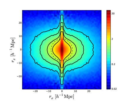
Because RSD effects only distort the observed coordinates (or pair separations) in the LOS direction, the two-point correlation function is fundamentally a function of two variables. In Fig. 1 we choose as coordinates the LOS separation, , and the separation transverse to the LOS, to display our measurement from the galaxy sample analysed in the present work. This measurement uses the angular upweighting method described in Sec. 4.1 to correct for fiber collisions. Two primary features are apparent: on large scales ( Mpc and above), contours of constant are “squashed” in the LOS direction. The correlation between the density and velocity field described by Eq. 3 on average reduces the apparent separation between pairs of galaxies along the line of sight. On smaller scales where Eq. 3 breaks down, the contours are instead stretched along the LOS. Galaxies orbiting in the potential of a gravitationally bound dark matter halo have a virial-like velocity component. As we will see, the SDSS-III CMASS galaxies shown here occupy massive dark matter halos with large virial velocities. The prominent feature in along the LOS (i.e., at Mpc) is due to these motions, often called “fingers-of-god” (FOGs) (Jackson, 1972); note that these virial-like velocities distort at all separations, and their impact must be mitigated even in analysis of relatively large scales (e.g., Reid et al., 2012).
In this work we choose not to analyse directly, since information is spread over a large number of bins. As described in Sec. 5.1, we estimate measurement errors by bootstrapping the survey, and therefore need to reduce the number of measurements to well below the number of bootstrap regions, which are limited in number since each region must span scales larger than we include in our analysis. In this section we present the observables we will estimate from and compare with theoretical models directly.
The most widely used observable in studies of small-scale galaxy clustering is , which quantifies the clustering as a function of transverse pair separation . All pairs with line-of-sight separations smaller than contribute to :
| (5) |
is traditionally chosen to be large (80 Mpc in this work) so that the sensitivity of to redshift space distortions is minimal (but see van den Bosch et al., 2013).
On large scales and for the highly biased tracers we consider here, the majority of redshift space information is available by measuring the first two even multipoles () of :
| (6) |
where redshift space separation is defined by and is the cosine of the angle of the galaxy pair with respect to the line of sight. Here is the Legendre polynomial of order . Both our measurement and theoretical estimates of are computed by replacing the integral with a direct sum over bins of width . Each bin in redshift space separation is averaged over a finite band of separations.
To mitigate the effect of fiber collisions, our primary analysis uses the statistic which approaches on large scales, but eliminates all bins that include pairs with Mpc. This choice corresponds to pairs separated by the fiber collision radius 62” at the maximum redshift included in our analysis, . Heuristically, we estimate
| (7) |
In practice, our implementation is slightly more complicated, but we emphasize that the measurement and theoretical predictions are computed with exactly the same algorithm, and so the details are irrelevant for the comparison of the two. We start with relatively fine logarithmic binning in () and () to compute . We then aggregate pair counts in the small bins into larger bins for which we report our measurements. In the case where some of the small bins have larger than the cutoff, we estimate in the larger bin from only that subset of small bins. If none of the bins have large enough in the -bin, we set for that bin to 0 before integrating over to estimate ; this is equivalent to only integrating up to a that is different for each fine bin. The previous step ensures that no pairs with smaller than the fiber collision scale are included. The exact and boundaries for our final bins are listed in Table 3.
2.4 -body simulation Halo Catalogs
| Parameter | LowRes | MedRes | HiRes |
|---|---|---|---|
| ( Mpc) | 2750 | 1380 | 677.7 |
| ( ) | |||
| 0.274 | 0.292 | 0.30851 | |
| 0.0224 | 0.022 | 0.022161 | |
| 0.7 | 0.69 | 0.6777 | |
| 0.95 | 0.965 | 0.9611 | |
| 0.8 | 0.82 | 0.8288 | |
| 0.550 | 0.550 | 0.547 | |
| 0.455 | 0.472 | 0.482 |
We make use of three periodic -body simulation sets throughout this paper. We have a single realization for the LowRes and HiRes cases, and three independent realizations (labelled 0,1,2) in the MedRes case. The simulation parameters are listed in Table 1. The LowRes box has parameters favored by WMAP7 (Komatsu et al., 2011), while the HiRes box adopts the “Planck+WP+highL+BAO” constraints from the Planck analysis (Planck Collaboration, 2013); all -body simulations assume massless neutrinos, while the parameter constraints from Planck assume eV. The Planck best fit and HiRes cosmologies will therefore have slightly different expansion and structure growth histories which should be negligible for the present application. The MedRes cosmology is “between” LowRes and HiRes. For each simulation we generate spherical overdensity (SO) halo catalogs using an overdensity of relative to the mean matter density to define the halo virial radius . Our catalogs extend down to fifty particles per halo where necessary. We use the Tinker et al. (2008) implementation of the SO halo finder, which allows halo virial radii to overlap, as long as the center of one halo is not within the virial radius of another halo; this choice alters the halo-halo clustering on scales near compared with a friends-of-friends halo catalog, in which two such halos would be bridged into a single halo (see figure 9 of Reid & Spergel, 2009).
More specifically, halos are identified around pseudo-peaks in the density field, which may or may not be located on the true density peak of the host halo. A radius is computed for each pseudo-peak in the density field within which the density is 200. Starting at a radius of 1/3 the initial , the center of mass is computed within this restricted radius and iterated to convergence. If the pseudo -peak lies on a subhalo, this procedure migrates the halo center to the true host halo density peak. Once convergence is reached, the top-hat radius is incrementally reduced and the center of mass is recomputed until the top-hat radius is /15.9 or the number of particles within the top-hat radius drops below 20. The center of mass is again computed iteratively at the tophat radius of /15.9. For halos above the 20 particle limit, this algorithm averages over of all halo members. This algorithm was originally refined to accurately locate the halo center; we verified that it recovers the position of the potential minimum within the halo to within 0.01-0.02 Mpc. We denote the mean velocity of these densest particles as , and is our fiducial choice for the velocity of each halo’s central galaxy. This choice is by no means unique, and Appendix B shows that while there is strong evidence that the dense central region of the halo does have a bulk velocity with respect to the halo members, the rms offset between the “central” velocity and the center-of-mass velocity depends on the radius over which the average is taken. The effective radius for our definition ranges from 0.04 - 0.08 Mpc for halos with in our MedRes simulation; this mass range hosts 90% of the central galaxies in our sample for our best fit halo occupation distribution model. The median seeing-corrected effective radius of CMASS targets is 1.2” (Masters et al., 2011), or 0.0087 Mpc. For a de Vaucouleurs profile, 0.04 (0.08) Mpc would contain 87% (96%) of the light. Therefore, our choice of central velocity definition is reasonably well matched to the typical extent of our target galaxies. Of course, since our simulations contain only dark matter, any impact of baryonic physics on the central dynamics has been neglected.
The LowRes box provides a volume much larger than the survey we analyse. To match the observed clustering strength using the LowRes box, we require halos below the SO halo catalog threshhold; for this purpose, we use a friends-of-friends (FOF) algorithm with linking length 0.168 to identify halos (Davis et al., 1985), and then compute their masses in a spherical aperture at . We further rescaled the FOF-derived halo masses by a factor of 0.975 to approximate masses used in the SO catalogs. The FOF catalog extends down to . Typically only of the mock galaxies are assigned to FOF-derived halos, so the impact of these details should be minimal. This hybrid catalog did show evidence for numerical artefacts in the halo clustering, which led us to adopt higher resolution simulations for our primary parameter constraints. The HiRes box provides more than sufficient mass resolution but its small volume made the theoretical predictions somewhat noisy. Because this box is smaller than our survey size, we have to add a theoretical error budget to the observational one. We use mock catalogs derived from the LowRes box for two applications. First, we generate a mock catalog to which we apply the BOSS tiling algorithm in order to investigate the fiber collision effects on clustering (see Sec. 4). Second, we subdivide the LowRes box into 64 subboxes to estimate the theoretical uncertainty due to the finite volume of the HiRes box.
3 Data
In this paper we analyse data included in data release 10 (DR10) of the Sloan Digital Sky Survey (SDSS; Gunn et al., 1998; York et al., 2000; Gunn et al., 2006; Eisenstein et al., 2011). We refer the reader to Ahn et al. (2013) for the full details about the DR10 dataset. Briefly, BOSS uses imaging data available in SDSS data release 8 (Aihara et al., 2011) to target quasars and two classes of galaxies for spectroscopy. The larger CMASS sample analysed in this work covers , but as in Anderson et al. (2013) we restrict our analysis to the subsample falling within . The LOWZ galaxy targets primarly have and so we treat them as uncorrelated with the CMASS targets.
Errors in the redshift fitting to the BOSS spectra propagate as random errors in the LOS redshift space position of each galaxy. The median redshift error reported by the BOSS spectroscopic pipeline is 0.00014. Bolton et al. (2012) estimate that these errors are underestimated by . While the redshift error increases with (by 40% between the lower and upper third of the sample), the conversion to distance errors partially cancels this. We therefore expect a typical line-of-sight offset of Mpc due to redshift errors. We incorporate redshift errors into our theoretical model by adding a random LOS offset to each mock galaxy that is drawn from a Gaussian distribution of width Mpc.
Throughout we treat the North and South galactic cap regions of the survey separately. Photometric calibration across the hemispheres is subject to systematic error, and may result in slightly different populations of galaxies being targeted in the two hemispheres; see Ross et al. (2012) for a more detailed analysis of potential differences. We will address the consistency of the north and south for each statistic we compute, and combine them before performing fits. The majority of our sample is contained in the north: 409365 of the 521958 galaxies in the final sample.
In Anderson et al. (2013) we upweighted nearest neighbor galaxies to account for two potentially non-random sources of missing redshifts: fiber collisions and failure to obtain redshifts for targets assigned a spectroscopic fiber. We adopt the same weighting procedure for redshift failures in present work. For fiber collisions, we assign a nearest neighbor redshift to each collided galaxy, drawn from another CMASS target within the fiber collision group provided by the tiling algorithm. In total, we corrected for 7043 (2829) redshift failures in the north (south) and 24648 (6297) fiber collided galaxies. The survey completeness is treated as uniform in each sector, which is defined as a unique intersection of spectrosopic tiles. The angular mask is defined in the same way as in Anderson et al. (2013), except that for the purposes of fiber collision correction uniformity, we only retain sectors where all planned spectroscopic tiles have been observed. We track two values of completeness in each sector. For , collided galaxies are assigned a nearest-neighbor redshift and treated as observed when estimating completeness. To define the completeness used in the angular upweighting method (Sec. 4.1), fiber collided galaxies are instead treated as a random subsample of the spectroscopic sample that lack redshifts, so they reduce the completeness of their sector. The area-weighted completenesses are and in the north (south). Finally, we note that we neglect both the FKP and systematics weights adopted in Anderson et al. (2013) so that galaxies receive equal weight in both the angular and three-dimensional clustering measurements. The systematics weights primarily affect clustering on very large scales, and can therefore be neglected on the small scales of interest here.
In order to place the observed angular and redshift coordinates of each galaxy on a comoving grid, we adopt the same fiducial cosmological model as in Anderson et al. (2013): . We compute from the Landy-Szalay estimator (Landy & Szalay, 1993), which depends on the data-data (), data-random (), and random-random () pair counts in each separation bin of interest:
| (8) |
Random galaxies are an unclustered sample of points within the survey mask with the same sector-by-sector completeness as the data and with a radial selection function matched to the data by drawing the random galaxy redshifts from the observed ones (i.e., the “shuffle” method advocated in Ross et al. 2012). In contrast to some other works that use weighting, we combine clustering statistics estimated separately in the two hemispheres using a simple weighted average with weights proportional to the total galaxy weight in each hemisphere.
4 Fiber collision corrections
The tiling algorithm (Blanton et al., 2003) determines the location of the spectroscopic tiles and allocates the available fibers among the galaxy and quasar targets. A physical constraint of the instrument is that fibers may not be closer than 62” on a given spectroscopic tile. The algorithm divides target galaxies into friends-of-friends groups with a linking length of 62”, and then assigns fibers to the groups in a way that maximizes the number of targets with fibers. The choice of which galaxies are assigned the fibers is otherwise random. The algorithm adapts to the density of targets on the sky, with a net result being that regions covered by more than one tile have a larger than average number density. For the DR10 sample studied in this work, 42% (52%) of the area in the north (south) is covered by multiple tiles, and the number density is larger by 4.6% (3.1%) in those regions. For the final survey footprint, the enhancement is 5.1% in both the north and south. Fiber collisions are partially resolved only in the multiple tile regions, and therefore may not be representative of the unresolved fiber collisions in lower target density regions. For this reason we do not adopt the method of Guo, Zehavi, & Zheng (2012), which uses the overlap regions to correct fiber collisions in the single tile regions.
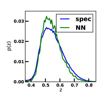
Fiber-collided galaxies cannot simply be accounted for by reducing the completeness of their sector, since they are a non-random subset of targets (conditioned to have another target within 62”). This is evident in Fig. 2, where we compare the redshift distribution of all good CMASS redshifts with the redshift distribution of the nearest neighbor of fiber collided galaxies; the latter preferentially reside near the peak of , where is also the largest. In this section we will apply the tiling algorithm to a mock galaxy catalog in order to assess the robustness of our fiber collision correction methods to the existence of realistic tile position-target density correlations. Finally, we note that fiber collisions also occur between CMASS targets and targets from other classes. Since quasar targets are given higher priority, we account for them by simply including a 62” veto mask around each high priority quasar target. CMASS targets that are fiber collided with LOWZ galaxies are treated as random losses; the completeness of their sectors is reduced accordingly, rather than assigning them a nearest neighbor redshift.
4.1 The angular upweighting method
The comparison of the angular clustering of the target galaxies with the angular clustering of the subsample of targets for which spectra were obtained quantifies the number of pairs lost as a function of angular separation due to fiber collisions. One common method to use this information to correct measurements of is to first treat the fiber-collided missing galaxies as if they were a random subsample of targets (i.e., adjust the completeness of the sector based on the fraction of targets without spectra), and then to upweight pairs in the Landy-Szalay estimator (Eq. 8) using the following weight (Hawkins et al., 2003):
| (9) |
Here is the angular correlation function of galaxies drawn from the “spectroscopic” sample for which you obtained redshifts and want to estimate . is the angular correlation function of the targets from which the spectroscopic sample is drawn.
As we will show using our tiled mock catalog, this method performs quite well at recovering the true clustering down to scales well below the BOSS fiber collision radius, and has been successfully applied in a number of other surveys (Hawkins et al., 2003; Li et al., 2006; Ross et al., 2007; White et al., 2011; de la Torre et al., 2013). However, there are a number of open issues and limitations of the method:
-
•
The method assumes that the distribution of LOS separations of the fiber-collided pairs is the same as the distribution for non-collided pairs; this will not be true in detail, since fiber-collided pairs may occupy a different distribution of halo masses (and therefore have a different large-scale bias) compared to the full target sample. Since quickly approaches 1 on large scales, the method will not properly account for the possibility of fiber-collided galaxies having a larger bias. For this reason we prefer the next method (nearest neighbor redshift assignment) on scales well above the fiber collision scale.
-
•
The weight given in Eq. 9 is not easily generalizable to “spectroscopic” samples that are subsets of the full set of fibers (in our case, cutting out stars and applying redshift boundaries), at least not without additional assumptions regarding the redshift dependence of the target galaxy clustering.
The Limber approximation (Limber, 1954) allows us to relate the angular and real-space clustering given the probability distribution that an object in the sample is at comoving distance .
| (10) |
Here is the LOS separation between a pair. The explicit dependence of in Eq. 10 indicates that may evolve with redshift. We can only observe for the full target sample. However, if we adopt a particular model for , then in principle we can fit for its parameters and infer the expected for a subsample of targets occupying a narrower range of (i.e., different ). The simplest choice is a power law correlation function, . In that case, Eq. 10 gives with
| (11) |
For a more complicated , in different redshift slices must generically have a different dependence that depends on . To relate the observed to the one for the subsample entering Eq. 9, Hawkins et al. (2003) employed the Limber approximation, assuming a power law form for and that it does not evolve with redshift. We make the same assumption in Sec. 5.2 but propagate the uncertainty in this step to our final clustering measurements.
4.2 Nearest neighbor redshift (NN) and Anderson et al. (2013) weighting schemes
An alternative fiber collision correction method is to simply assign a fiber-collided galaxy the redshift of its nearest neighbor (labelled NN in subsequent figures). In the limit of separations large compared to 62”, this is equivalent to the method employed in our large-scale analyses, and described in detail in Anderson et al. (2013). In that work we assign the weight of a fiber collided galaxy to its nearest neighbor, which is propagated into the redshift distribution and correlation function calculations. A nice property of this method is that it is guaranteed to recover the correct large scale clustering amplitude of the full sample, at least in the limit of fiber collision pairs rather than groups. While the large scale bias is considered a nuisance parameter in galaxy auto-correlation analyses, it is used in cosmological parameter analyses when comparing galaxy clustering with galaxy-galaxy lensing, for example in the test (Reyes, 2010). This method will not recover accurate statistics on small scales, since the LOS separation between the collided and nearest neighbor galaxy will be artificially set to 0, thus suppressing true FOGs in the galaxy sample.
4.3 Solution using a tiled mock catalog
We generate a mock catalog covering the northern galactic cap portion of the SDSS-III BOSS survey using the LowRes simulation box listed in Table 1. The HOD parameters for this mock catalog were chosen based on a preliminary fit to preliminary measurements of : , , , , and . The central galaxy velocities were defined using , the center-of-mass velocity of the host halo. We also set and in order to get a reasonable fit to the observed clustering. All of these HOD parameters are described in detail in Sec. 6. In the following section we compare the clustering in the mock catalog with the data; the agreement is not perfect but sufficiently good for our purpose, which is to compare various fiber collision correction methods against the true clustering in the mock catalog.
We choose the number density of the HOD to be ( Mpc)-3, larger than the maximum value of the CMASS sample and first generate a uniform mock catalog using a single redshift output. We then apply the angular mask of the NGC for the final BOSS survey, and randomly downsample the mock galaxy catalog to match the observed CMASS . We keep galaxies between in the mock catalog to account for the difference between the angular clustering of the full target sample and the angular clustering of the targets after applying the redshift cut . Note that this mock catalog therefore meets the “constant clustering” assumption discussed in Sec. 4.1. This broader redshift coverage incorporates the vast majority of CMASS targets except for the 3% of targets that are stars. We make use of the approximate independence of the LOWZ and CMASS galaxy distributions, and input the positions of the true LOWZ and quasar targets before applying the BOSS tiling algorithm to the mock catalog. We measure the for the full mock target sample and for the mock target sample after applying redshift cuts, and find that on all scales of interest their ratio remains within 1% of 1.14, the value expected from Eq. 11. We also find that the angular weight that estimates from the set of all targets assigned to fibers (and corresponds to the full target sample) returns the same weight as our fiducial approach with redshift cuts, within 1%.
As we quantify in more detail in Sec. 5 and Fig. 8, our tiled mock catalog shows that the angular upweighting method recovers the true within 1.5% on all scales, while the same is true above the fiber collision scale when using the nearest neighbor redshift method. Similarly for the statistics, the nearest neighbor method almost perfectly recovers the true clustering above Mpc. The angular method is nearly unbiased on scales below Mpc, but shows systematic differences on intermediate scales for both and . Our final clustering estimators will use the nearest neighbor method on large scales and angular upweighting on small scales to infer the clustering of the CMASS sample in absence of fiber collisions, with systematic uncertainty below the statistical one. Therefore, we are not compelled to introduce any more complicated fiber collision correction schemes, such as the one recently proposed in Guo, Zehavi, & Zheng (2012). However, we note that their tests corroborate our findings that angular upweighting performs well on scales below the fiber collision scale, and the nearest neighbor method is unbiased on large scales. We note that their method has not yet been verified on a mock catalog with realistic tile-density correlations.
5 Measurements and Covariances
5.1 Survey Bootstrap Regions
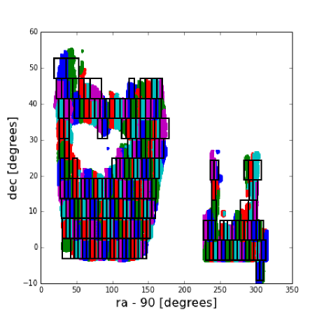
We derive statistical covariances on our measurements by dividing the survey into 200 subregions, roughly equal in size and shape. Fig. 3 shows the regions. To define them, we first distributed square regions across the survey footprint with sidelength 5.56 degrees using dec, ra coordinates. At in our fiducial cosmology this corresponds to 145 Mpc on a side and the redshift extent from to translates to 608 Mpc. For comparison, the largest separations included in our measurements is 38 Mpc, and our measurements extend along the LOS to 80 Mpc. Along each row of constant dec, we shifted the square centers in the ra direction to maximize the number of “nearly full” squares. We then grouped neighboring squares together in order to homogenize the number of galaxies per bootstrap region. Finally, galaxies and randoms outside any of the 200 bootstrap region were assigned to the nearest regions. The final distribution of randoms per bootstrap region had a one- scatter of , accounting for both survey footprint incompleteness in the regions and variations in completeness for regions within the survey footprint. To derive bootstrap errors, we compute each observable separately in each subregion, excluding pairs that cross subregion boundaries. We use a single normalization between the data and random counts (though different for the north and south) that enters the Landy-Szalay estimator; this choice uses information from the entire survey to constrain the expected number density of galaxies as a function of redshift. The bootstrap covariance is then estimated as
| (12) |
and we set . Here is the mean of randomly selected (with replacement) from the subregion measurements.
Following Hartlap, Simon & Schneider (2007), we estimate the inverse covariance matrix as
| (13) |
but see discussions in Krause et al. (2013) and Eifler, Kilbinger, & Schneider (2008). In our case , and = 27 for our default analysis, which jointly fits and . We verified that covariances derived by dividing the survey into a smaller number of boostrap regions (50 or 100) gave similar correlation structure, and diagonal errors reassuringly agreed at the level for .
5.2 Angular clustering and fiber collision angular weights
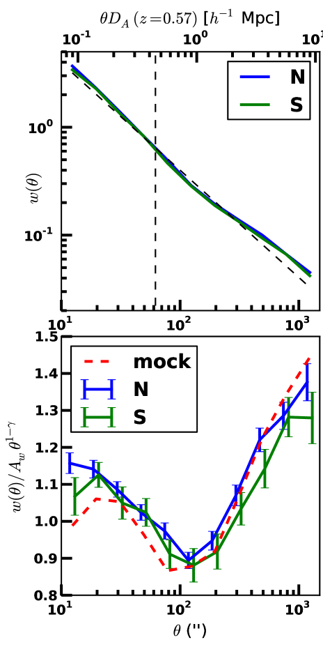
The angular clustering of CMASS targets in the northern and southern galactic caps is shown in Fig. 4. A power law is a reasonable description of the overall behavior, though level deviations are clearly detectable. We find for a power-law fit with 11 degrees of freedom. At ( 1 Mpc), there is a dip that corresponds to the one-halo to two-halo transition region in the halo model. We find that the difference between the north and south measurements of is consistent with our bootstrap errors, so there is no indication in this statistic that the galaxies in the two hemispheres we select cluster differently.
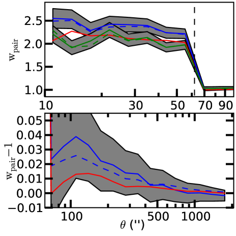
In this paper we analyze a single redshift-selected subsample of CMASS targets, . 8% (9%) of targets in the north (south) are galaxies that fall outside this redshift range, with in Eq. 10 of these discarded targets peaking in a relatively narrow range in near both redshift boundaries. Another 2.6% (3.1%) of targets are stars (neglected in the mock tiling), and their angular clustering is weak enough to be completely neglected on these scales. Following Hawkins et al. (2003) and White et al. (2011), we use Eq. 11 to relate the observed clustering of the full target sample (shown in Fig. 4) to the expected target clustering after the redshift cuts. We find is 1.18 (1.2) in the north (south) under the “constant clustering” assumption that targets inside and outside the redshift cuts have identical real-space clustering. If we instead assume that outside our redshift cuts, this factor would be reduced by 6% (8%). Measurement of for the galaxies outside our redshift cuts is noisy, but indicates that the constant clustering assumption is correct, within a factor of . Therefore we assign a systematic uncertainty to in Eq. 9 of 10%, shown as the grey bands in Fig. 5. Finally, unlike Hawkins et al. (2003), we do not systematically shift the angular coordinate of in the full sample when estimating for the redshift subsample; a weighted mean of yields a difference of only 0.1% in the subsampled case. Our final estimates of the angular correction for the north (blue solid line) and south (green solid line) are shown in Fig. 5. The plate density in the south is slightly higher, so the angular weight is smaller than in the north on scales below the fiber collision radius. We also show the angular weight derived in the same manner using the tiled mock catalog (red). In the tiled mock catalog, the constant clustering assumption is accurate by construction. In all three cases, the weights quickly approach 1 above the fiber collision scale. For comparison, the dashed lines show angular weights derived setting to the full sample of targets that were assigned fibers, and to the full target sample, as opposed to our fiducial method of estimating both after applying redshift cuts. Within our 10% uncertainty in , the two schemes are identical. We propagate the uncertainty in the angular pair weight by computing the statistics of interest (, , and ) with our best estimate of as well as derived from changes in in Eq. 9.
5.3 Projected correlation function
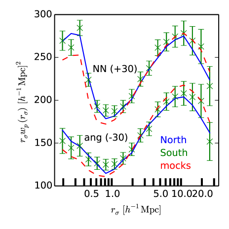
In Fig. 6 we show our measurements of in the northern (blue) and southern (green) hemispheres of the DR10 CMASS sample, compared with the tiled mock catalog (red). Errors on the south measurements are square root of the diagonal elements of the bootstrap covariance matrix after dividing by the fraction of total galaxies in the south. To assess the consistency of the two observations, we compute
| (14) |
Assuming that the bootstrap covariance matrix can be rescaled using the total galaxy weight in the (independent) northern and southern subsamples to adequately describe the data covariances, we would expect
| (15) |
where () are the total number of galaxies in our sample in the north (south). For , . We find (expected 106) for the estimated using nearest neighbor redshifts, and similar results for the angular upweighting method, so the two are perfectly consistent. We also compute between the combined N+S measurement and the tiled mock result; (91) for the nearest neighbor and angular upweighting statistics, respectively, while we expect 73. The disagreement is worst in the nearest neighbor redshift case on the smallest scales, where we will adopt the angular upweighting result for our final analysis.
5.4 Anisotropic clustering measures and
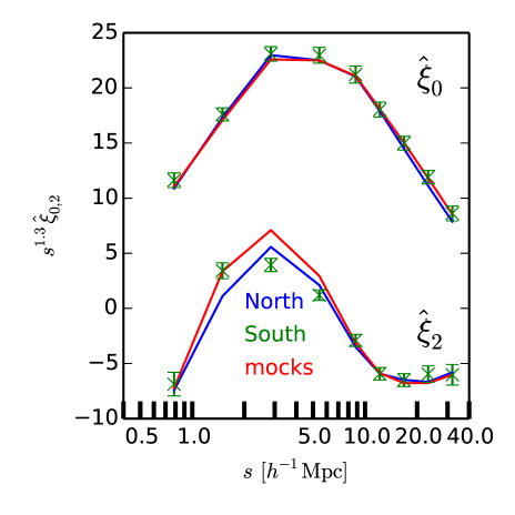
Fig. 7 shows a comparison of measured from the north, south, and tiled mock catalog using the nearest neighbor redshift correction; results for angular upweighting and for are very similar. Applying Eq. 14 to the disagreement between the north and south subsamples is larger: (expected 106) but within the expected variation for this quantity. Comparing from the tiled mock catalog to the data we find agreement for both angular upweighting and nearest neighbor redshift, which should be more than adequate for measuring the small differences between the true clustering and the clustering estimated from those correction methods.
5.5 Best estimators derived from tiled mocks and systematic uncertainties
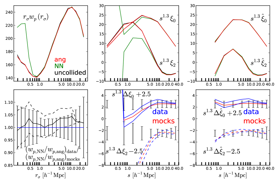
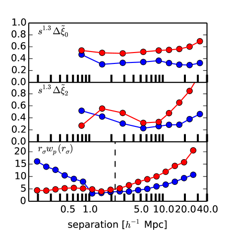
As argued in Sec. 4.2, the nearest neighbor redshift assignment method (“NN”) should provide nearly unbiased clustering estimates on large scales, as long as one avoids small contributions, so we will rely on this method on scales well above the fiber collision scale. On smaller scales angular upweighting (“ang”) method is more accurate. In Fig. 8 we compare the underlying “uncollided”, complete target catalog (black) with the nearest neighbor redshift (green) and angular upweighting (red) methods for recovering the underlying clustering. In this figure we investigate the three statistics of interest, , , and . On small angular scales the angular upweighting method does indeed recover the underlying clustering at high accuracy for all three statistics, while the nearest neighbor method is effective only on larger scales. The comparison between the middle and right panels illustrates the large contribution of the scales to the multipoles . Eliminating those scales brings the nearest neighbor and angular upweighting estimators into very good agreement for the statistic, which is why we choose to include it rather than in our parameter fitting. With this comparison in hand, we define our best estimate of these statistics from the data in the following way. For each statistic (, , , , ), we use the difference between the two estimators and the “truth” to determine a transition scale at which we switch from the angular estimator on small scales to the nearest neighbor redshift estimator on large scales; we find (1.09, 8.8, 12.2, 1.5, 1.5) Mpc. Next, we use the difference between the estimator and “truth” in the mock catalogs as an estimate of the bias of the observed statistics. We subtract this difference from our measurements, and add its square to the diagonal elements of the bootstrap covariance matrix. For this correction is completely negligible. For it is except for , for which the shift is ; here refers to the diagonal element of the bootstrap covariance matrix. This difference is slightly larger than for in the range 5.4-12.2 Mpc. For points using the angular upweighting method, we translate the uncertainty in the angular weights, shown in Fig. 5, into an additional uncertainty on the measured statistics. We add this source of uncertainty to the diagonal of the bootstrap covariance matrices, which were computed using fixed angular pair weights. This increases the diagonal uncertainty on the clustering by a factor of two or more for the points affected. The resulting estimate of as well as the diagonal uncertainty is tabulated in Table 2, and and are listed in Table 3.
In the lower set of plots in Fig. 8, we compare differences in all three statistics using the nearest neighbor redshift and angular upweighting method measured in both the mocks and the data; for comparison, we show diagonal uncertainties from our final covariance matrix presented in Sec. 5.6. Differences between these two observables are determined by the redshift distribution and clustering properties of the galaxy sample as well as the tiling algorithm. These differences seen in the data are reproduced with good accuracy by our mock catalogs.
In the left panel we compare the ratio of , which is large below the fiber collision scale and approaches 1 on large scales in the mocks. The data behaves similarly, but with a relatively constant factor offset with the mocks. This offset is within the reported angular upweighting uncertainty (dashed curves) and also small compared to our final error budget. In the middle and right bottom panels we show instead the difference ; the same offset in is also present in and . The blue curves in these panels show the allowed region after propagating our 10% uncertainty in the angular weights, and the red curves show the differences measured from the mock catalogs. They are consistent within the uncertainties.
| 0.195 | 1000.5 | 85.6 | 2.60 | 73.8 | 2.5 |
| 0.260 | 691.7 | 56.2 | 3.46 | 59.8 | 2.2 |
| 0.346 | 507.7 | 39.2 | 4.62 | 48.4 | 2.0 |
| 0.462 | 358.1 | 25.3 | 6.16 | 38.0 | 1.7 |
| 0.616 | 252.4 | 17.1 | 8.22 | 29.6 | 1.4 |
| 0.822 | 179.8 | 11.5 | 10.96 | 22.3 | 1.2 |
| 1.096 | 140.3 | 5.2 | 14.61 | 15.9 | 1.1 |
| 1.461 | 111.0 | 3.5 | 19.48 | 11.2 | 0.9 |
| 1.948 | 88.5 | 3.1 | 25.98 | 7.4 | 0.9 |
| 0.234 | 0.097 | 0.569 | 0.000 | 0.000 | 57.757 | 4.428 | - | - | 60.471 | 7.699 | - | - |
| 0.785 | 0.569 | 1.084 | 0.345 | 0.845 | 24.665 | 1.497 | 14.339 | 0.913 | 30.726 | 2.744 | -8.346 | 0.767 |
| 1.496 | 1.084 | 2.065 | 0.870 | 0.955 | 12.841 | 0.555 | 10.363 | 0.317 | 11.687 | 1.037 | 1.094 | 0.382 |
| 2.851 | 2.065 | 3.936 | 0.965 | 0.985 | 6.403 | 0.208 | 5.865 | 0.139 | 3.811 | 0.300 | 1.309 | 0.134 |
| 5.433 | 3.936 | 7.499 | 0.990 | 0.995 | 2.559 | 0.077 | 2.503 | 0.063 | 0.633 | 0.080 | 0.212 | 0.040 |
| 8.810 | 7.499 | 10.351 | 0.995 | 0.995 | 1.273 | 0.037 | 1.244 | 0.035 | -0.074 | 0.043 | -0.197 | 0.023 |
| 12.162 | 10.351 | 14.289 | 0.995 | 0.995 | 0.707 | 0.023 | 0.696 | 0.023 | -0.185 | 0.023 | -0.227 | 0.020 |
| 16.788 | 14.289 | 19.724 | 0.995 | 0.995 | 0.377 | 0.015 | 0.374 | 0.015 | -0.151 | 0.017 | -0.164 | 0.017 |
| 23.174 | 19.724 | 27.227 | 0.995 | 0.995 | 0.190 | 0.010 | 0.189 | 0.010 | -0.103 | 0.015 | -0.107 | 0.014 |
| 31.989 | 27.227 | 37.584 | 0.995 | 0.995 | 0.088 | 0.008 | 0.088 | 0.008 | -0.062 | 0.013 | -0.063 | 0.012 |
5.6 Combined measurement and theory covariance matrix
So far we have accounted for three sources of uncertainty in our measurements: the standard finite volume sampling, for which we estimate a full measurement covariance matrix using the 200 bootstrap regions in Fig. 3; 10% uncertainty in the angular weights used in the angular upweighting method, which we propagate to the observables of interest and then add to the diagonal elements of the covariance matrix; and systematic uncertainty equal to the size of debiasing correction derived from the mock tiling catalog and added to the diagonal elements of the covariance matrix. The combination of these three terms we call our “measurement” uncertainty. One final source of statistical error comes from uncertainty in our theoretical prediction. The total volume within the DR10 survey mask after applying our redshift cuts is ( Gpc)3, though some of this volume is mapped with a low number density of galaxies. The HiRes -body simulation box, for which we estimate the theoretical error, covers only of that volume. Our theoretical calculation averages over all possible realizations of a particlar HOD (for the given halo catalog), which removes much of the sampling variance from the theoretical calculation. Cosmic variance assoicated with the underlying dark matter realization remains, but the theoretical error will be smaller than the naive volume comparison suggests.
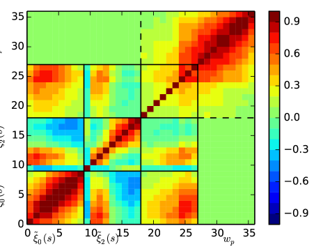
In order to estimate the theoretical uncertainty, we populate the LowRes simulation halo catalogs with the same HOD as in Sec. 4.3. We divide the box into subboxes the size of the HiRes box, which allows for a Mpc buffer between subboxes in each direction. We again include the factor in Eq. 13 with to unbias the inverse bootstrap covariance matrix estimate; for , the prefactor is 1.8. More simulation volume could reduce both the theoretical uncertainties and covariance, but is only justified if we have not reached a systematics floor in the theoretical modeling. The left panel of Fig. 9 compares the diagonal elements of the final “measurement” uncertainties with the theoretical uncertainties. We sum the measurement and theory covariance matrices to arrive at our final covariance matrix that we will invert and use in a standard analysis to do model parameter fitting. In the right panel, we show the correlation matrix for the . As is true on large scales as well, neigboring bins in are highly correlated, meaning the data is relatively insensitive to overall changes in the amplitude of clustering, but more sensitive to spatially-abrupt model signatures (like the BAO feature). The bins are less correlated than for large separations, and there is significant covariance between all three observables. At large separations, becomes negative, so a positive correlation in the amplitude of the multipoles (as we would expect from uncertainty in an overall bias factor) shows up in that region as an anti-correlation.
6 Model
The only detailed semi-analytic HOD based descriptions of galaxy clustering in redshift space available to our knowledge are given in Tinker (2007) and Zu & Weinberg (2012). The models presented therein require a description of the probability distribution of pairwise halo line-of-sight velocities as a function of their real space separation, orientation with respect to the line of sight, and the two halo masses. These distributions have substantial skewness and kurtosis that depends on pair separation and halo masses. These semi-analytic models require calibration of several scaling relations against -body simulations; fine-tuning or extending it to reach the precision demanded by our measurements would likely be extremely challenging.
Throughout the present analysis we therefore resort to deriving our theoretical predictions directly from mock galaxy catalogs based on -body simulations, as detailed below. The disadvantage of this approach is that cosmological parameter dependences are not easily incorporated, and the theory evaluation must be fast enough to permit at least a five-dimensional Monte-Carlo HOD parameter exploration. Following Neistein & Khochfar (2012) we implemented a pre-calculation of pair counts in fine mass bins; sums over these counts allow fast evaluation of the theoretical prediction as a function of HOD parameters. However, parameters that alter the velocity of galaxies change all pair separations and therefore require recalculation of the pair counts. We explored interpolation of the pair counts across the set of three velocity parameters described in Sec. 6.3. While useful for determining parameter degeneracies and expected uncertainties, the resulting constraints were not sufficiently accurate given the coarseness of the velocity parameter sampling. We therefore resort to varying one or at most two velocity parameters simultaneously.
6.1 Halo and central velocities
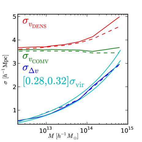
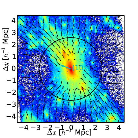
For a given SO halo catalog, we consider two definitions of halo velocities; these velocities are assigned directly to “central” galaxies, and the intrahalo velocity component for satellite galaxies is defined with respect to this halo velocity. The first choice is to simply average the velocities of all the halo members, denoted , for center-of-mass velocity. The dispersion of halo member velocities around the center-of-mass velocity is
| (16) |
fit to halos in the HiRes box; the HiRes and MedRes dispersions agree within 2% with this relation, the LowRes box within 5%. The three are in per-cent level agreement above . Therefore, within the range accessible to this study, the intrahalo velocity dispersions are independent of both cosmology and simulation resolution within a few per-cent, at fixed SO halo mass. The green curves in Fig. 10 show that the rms center-of-mass halo velocity is remarkably independent of halo mass (within 2% of 3.57 for halos in the HiRes box). The MedRes is lower by a factor of 1.016, in reasonable agreement with the linear theory expectation of 1.021 given the ratio of the values of for the two boxes.
The second central velocity definition, , was defined precisely in Sec. 2.4, and the sensitivity to this definition was explored in more detail in Appendix B. Note that in both catalogs we use that same density peak to define the halo center, where we place the “central” galaxy, so positions in the two halo catalogs we compare are identical; only the “central” galaxy velocities are different. Fig. 10 shows that the magnitude of rises with halo mass. If we consider the difference vector , we get the blue curves in Fig. 10. We see that depends on mass in the same way as the halo virial velocity (Eq. 16), but the magnitude is smaller by a factor of 0.3.
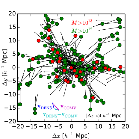
Fig. 11 illustrates these velocity vectors in the local environment of the largest halo in the HiRes simulation, which has . The real space coordinates have been shifted to place the halo at the (0,0) and projected into the plane defined by (blue) and (magenta). In the left panel we take a Mpc slice around the central halo and plot the positions (dots) and velocities (relative to of the central halo; black vectors) of halos within Mpc in and . The relative velocity of the dense clump of the central halo is shown as the cyan vector. In the right panel we examine the virial region (marked by the black circle) and surrounding structure with a log mapping of the density field. Mean matter velocities are shown with black arrows, scaled down by a factor of 20 for visualisation purposes. The net offset is shown as the cyan vector, scaled down only by a factor of two; it is inherently much smaller than the infall region velocities, and is correlated with a major filamentary structure. The correlation will be imprinted in since the relative velocity will preferentially move pairs along the filamentary structure and thus preferentially along their separation vector.
One final point of interest in comparing these vectors is that the difference vector contains a component along the direction, such that the magnitude of is larger in that direction by 1.5%. This provides a ballpark upper limit on how much the central galaxy velocity details may alter the effective on large scales, if the correlation is sourced by the quasilinear velocity component driving the large-scale Kaiser distortions. We propagate these two velocity choices to galaxy clustering predictions in Sec. 7.2. Further investigation is warranted beyond these two choices. However, given the good agreement between our “central” velocity definition and the more detailed phase-space investigation given in Behroozi, Wechsler, & Wu (2013), we assert that is the more physical choice of the two.
6.2 Number Density Prior and Redshift Evolution
Our HOD model based on a fixed redshift -body simulation halo catalog can only be an approximation to the real CMASS galaxy sample, for which the number density varies considerably across the redshift range of our sample; potentially the galaxy properties are redshift dependent as well (see earlier work on this topic in Masters et al., 2011; Ross et al., 2012, 2014). Remarkably, in Appendix A we find that there is no measurable redshift evolution in the statistic across the sample, even though the number density drops by a factor of 2.2 in the high redshift sample. We therefore take the simple ansatz that galaxies at all redshifts are a random subsample drawn from a single population. The observed simply reflects the fraction of the parent population selected by the CMASS targeting algorithm as a function of redshift. While a more complete model would allow all the HOD parameters to vary with redshift to match the observed , the data do not require it and it cannot be done without considerably increasing the complexity of our theoretical calculation (i.e., requiring the generation of light-cone halo catalogs).
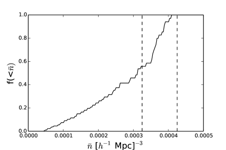
Fig. 12 shows the cumulative probability distribution of at the redshift of the galaxies in CMASS after applying the redshift cut . The vertical lines show the hard prior we assumed when fitting the single underlying HOD, in units of ( Mpc)-3. The lower bound is set by requiring the parent population to have higher number density than the typical CMASS galaxy. The upper bound depends on the completeness of our target selection, which in turn depends on the size of the photometric uncertainties in the imaging data. We have chosen a value safely above the peak of the number density distribution for the fiducial case, and will demonstrate in Sec. 7.6 that our constraints on are insensitive to this choice. As discussed in Sec. 7.6, the observed galaxy clustering amplitude and the abundance of sufficiently highly biased halos sets a hard upper limit of ( Mpc)-3.
6.3 Halo Occupation Distribution (HOD) parameters and implementation
The parametrisation of the HOD we adopt follows Zheng et al. (2005), and has been used in a number of studies focusing on the SDSS-II Luminous Red Galaxy sample (Reid & Spergel, 2009), the SDSS-III CMASS sample (White et al., 2011), and the SDSS-III LOWZ sample (Parejko et al., 2013). We separately model central and satellite galaxies, assuming that a central galaxy is required for a given halo to host a satellite galaxy. We model the probability for a halo of mass to host a central galaxy as
| (17) |
In our default model, the central galaxy is assigned to the position and velocity () of the density peak of its host dark matter halo. We also test a model with the same position assignment, but set the central velocity to . Given that a given halo of mass hosts a central galaxy, the number of satellites assigned to the halo is drawn from a Poisson distribution with mean
| (18) |
We set . The average total number of galaxies in a halo of mass is then
| (19) |
For each satellite galaxy we assign the position and velocity of a randomly chosen dark matter particle member of the host halo. When fitting for the HOD parameters we sample , , and so all masses are constrained to be larger than 0.
We also introduce three new parameters that rescale the galaxy velocities without altering their positions.
-
•
: This parameter rescales all halo velocities in the simulation. If linear theory were accurate on all scales, a fractional change in would be equivalent to a fractional change in the large-scale peculiar velocity field amplitude, . In Sec. 7.7 we demonstrate the validity of this approximation for relative halo velocities even on non-linear scales. Our constraints on are derived by interpolating across the theoretical model evaluated between in steps of 0.01. For our fiducial fit, the lower bound is away from the best fit.
-
•
: This parameter rescales the velocity of satellite galaxies relative to the host halo. Conceptually, this amounts to rescaling the virial velocity of the halo and/or accounting for sub-halo/galaxy velocity bias effects.
-
•
: This parameter specifies an additional random (Gaussian) dispersion for central galaxies in units of the halo virial velocity.
6.4 Interpreting in the halo model
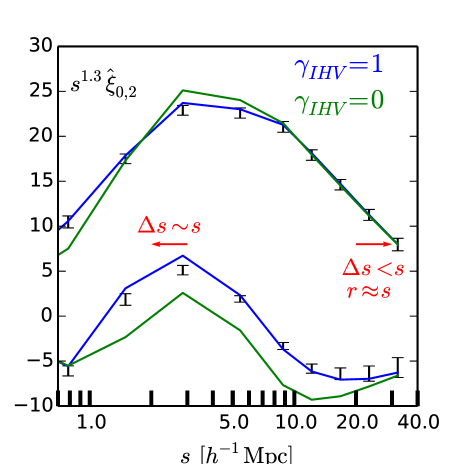
One prime advantage of the observable is that the x-axis (projected separation ) draws a neat separation between the two physical components of the halo model; the majority of pairs with smaller than the virial radius of the typical host halo actually occupy the same host halo (the “one-halo” term); on larger scales, pairs originate from different host halos (the “two-halo” term). Such a distinction is impossible at small redshift space separations . Although an extreme example, Fig. 11 illustrates the large intrahalo velocities on small scales, and how they blur the underlying small-scale structure. Using the results of Reid & White (2011), we find that halos of mass have a mean relative pairwise velocity of Mpc at separations below 10 Mpc and a pairwise velocity dispersion that increases with scale, also with an rms of Mpc at true (real space) halo separations of 5 Mpc. Thus we expect that below scales of Mpc, there is little correlation between the observed redshift pair separation and the true one; as shown in Fig. 13, this is the scale where transitions from positive to negative for the underlying halo distribution (see the green model curve where satellite velocities have artificially been set to 0).
Fig. 13 also shows that there is a plethora of information in on the satellite galaxy velocity dispersion. The satellite velocity dispersion distorts only below 10 Mpc. Removing the satellite intrahalo velocities lowers the quadrupole significantly on all scales of interest. The difference between an HOD model fit to the data and the same model without satellite velocity distpersions is 400.
7 Results
| fiducial | HiRes | HiRes | MedRes | COMV | COMV | high | |
|---|---|---|---|---|---|---|---|
| (18) | |||||||
| (18) | |||||||
| (27) | |||||||
| MedRes1 | MedRes2 | high | cen/sat test | MedRes0 | MedRes0 | MedRes0 | |
| (18) | |||||||
| (18) | |||||||
| (27) |
In this section we fit the measured and using the covariance matrix presented in Sec. 5.6 and Fig. 9 to the model described in Sec. 6. Our recommended constraints based on our best guesses regarding modeling choices (justified further below) are indicated in Table 4 as the bold “fiducial” column, while many other modeling choices are presented there only for comparison. We also indicate parameters held fixed in particular analyses by bold.
7.1 Choice of measurement combination and
In this analysis we study galaxy clustering on scales below the typical host halo virial radius, out to the quasi-linear scales used in our large-scale RSD measurements. The maximum scale included sets a limitation on the number of available bootstrap regions from the survey, and that, in turn, sets a limit on the number of observables for which we can reliably estimate a covariance matrix. It was thus our goal to determine a minimal set of observables that contained most of the available clustering information on the scales of interest. Initially we considered fits only to either or . We prefer the latter because of its insensitivity to fiber collision corrections and smaller uncertainties. We found that these two observables preferred distinct regions of HOD parameter space, at least in our fiducial HOD parametrization: fits to alone prefer a low satellite fraction of and did provide a better fit to the small-scale behavior of than presented below. However, this model was in strong tension with both and on small scales because of the low satellite fraction. We concluded that information relevant to the satellite HOD parameters was missing from , and so we decided to jointly fit Mpc) and to search for models that could fit both adequately. The number of elements in our data vector used throughout the rest of the paper is : the nine smallest scale bins in as well as nine bins each for and . The tension between the initial fits to and naively indicates shortcomings in our model; however, as we show in Sec. 7.3, we are able to find a model within our fiducial parametrisation that adequately fits all three observables.
We planned to use only the HiRes simulation box for our theoretical calculations, but given the noisiness of the resulting likelihood surface in , we verified our results by repeating the fits with three independent MedRes simulation boxes. Most of the final results we report are based on the MedRes0 box, but some cases using the HiRes box are presented for comparison. In general we found excellent agreement between the two.
7.2 Comparing and central galaxy velocity definitions
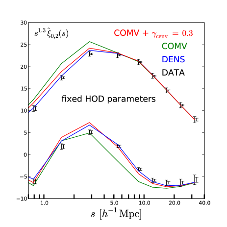
We first compare fits using two different central galaxy velocity choices, (default) and using the MedRes0 box. In this comparison central galaxy positions are fixed and only their velocities are varied. The prediction for from the best fit HOD model with (upper fourth column in Table 4) is shown in Fig. 14 in blue. To emphasize the differences caused by the choice of central galaxy velocity, we also plot the prediction for the same HOD using the center-of-mass halo velocity for central galaxies (green) and center-of-mass halo velocity plus a random Gaussian dispersion term consistent with the magnitude of (red); see Fig. 10. The model is clearly a bad fit, which is also true when the HOD parameters are allowed to vary. By eye, the difference between the fiducial model and does not appear large compared with the square root of the diagonal elements of the covariance matrix (larger errors in Fig. 14). However, the covariance matrix has very strong correlations; to give an alternate sense of the true constraining power of our measurements, we also show a second error bar, which is the size of the change required in a single bin to change by 1, when the model and theory differences are set to 0 in all other bins. The difference between these two “errors” is largest (a factor of 5) in the 5-17 Mpc bins of . Thus the data do show a strong preference for () compared with either (; upper column five of Table 4) or (; upper column six), when our HOD parameters are allowed to vary and assuming the underlying halo clustering in the simulation is sufficiently similar to that in the real universe. The latter comparison indicates that the motion of the dense core of the halo relative to the center-of-mass of the halo is correlated with the surrounding cosmic structure, and this correlation propagates into the shape of the correlation function; Fig. 11 shows the alignment between the velocity difference vector and the density field around the most massive halo in the HiRes simulation. The net effect of this density-velocity correlation is to increase the redshift separation between pairs, thus broadening both and compared to the uncorrelated dispersion case, . In Fig. 11, the difference vector - is oriented such that it will increase the redshift separation between the central halo and halos falling in along the corresponding filament. We saw similar levels of differences in the HiRes box compared with the MedRes box when performing the same test. These possibilities are certainly not the only choices for assigning velocities to galaxies and neglect all “gastrophysical” effects; however, the investigations in Behroozi, Wechsler, & Wu (2013) do indicate that our has similar properties to a more detailed phase-space based halo finding algorithm.
7.3 Goodness of fit
For our fiducial choice using and the MedRes0 box for the underlying halo catalog, and introducing no free HOD velocity parameters, we find for 27 data points and 5 free HOD parameters; a larger is expected only 2.5% of the time. This high could be an indication of insufficiencies of our model, non-Gaussianity of our errors, a preference for different cosmological parameters compared with our simulation parameters, or simply bad luck. For further insight, we attempt to fit MedRes and HiRes without the theoretical error contribution to the covariance matrix. If our theoretical predictions were based on single catalog realizations rather than an average over all possible HOD realizations for a fixed halo catalog, we would expect the contribution from the measurement and MedRes theory errors to be comparable because they cover comparable volumes. We find () to be compared with the fourth (second) columns in Table 4 for the MedRes0 (HiRes) halo catalogs. That is, our fiducial model seems adequate, within at least a factor of of the measurement errors. The fact that using the HiRes halo catalog, which covers only an eighth of the MedRes box volume, returns a better in this case must indicate that changes to the observables allowed by our theoretical uncertainties can be mostly absorbed by tweaking the HOD parameters. If that were not the case, we would have expected a much larger contribution from the higher theoretical uncertainty of the HiRes box to . The slight difference could also indicate a preference of the data for the higher-resolution halo catalog. In any case, these tests do not indicate the existence of systematic modeling errors at the level of our total quoted uncertainty. Of course, just because the model can fit the data does not demonstrate that the resulting parameter fits are unbiased.
7.4 Properties of the Halo Occupation Distribution
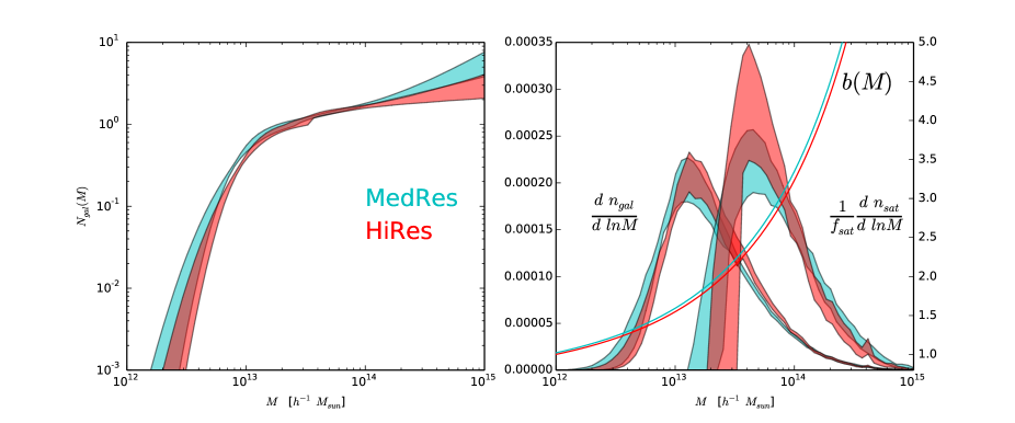
Figure 15 shows the
halo occupation distribution at the fiducial cosmologies of our HiRes and MedRes
boxes (corresponding to upper columns two and four in Table 4). We
enforce a hard prior on which does affect the
constraints from the HiRes box. Table 4 shows that the HOD
parameters are quite stable as we explore different parameter spaces and model
assumptions, with the exception of the “high ” and
“cen/sat test” cases detailed in the next section. Within the fiducial
prior discussed in Sec. 6.2, the data prefer
the largest allowed values of ; the best fit value is near
the hard prior upper boundary. Under the fiducial prior,
the fraction of galaxies that are satellites is strongly constrained: per-cent. The data show a strong preference for a non-zero
at a value of , which could plausibly be produced by a 1:1
merger of halos of mass . The distribution of galaxies across halo
mass is relatively symmetric as a function of (right panel of
Fig. 15), which makes the median (
) and mean ( ) host halo
masses quite different. For satellite galaxies, the median (mean) host halo
mass is .
The mean host halo mass is most closely related to the expected amplitude of the
galaxy-galaxy lensing signal. The amplitude of clustering of CMASS galaxies on
scales substantially larger than a typical host halo virial radius constrains
the product of a linear bias factor and the overall amplitude of matter
fluctuations at the effective redshift of the galaxy
sample. The observed for the CMASS galaxy sample places it in a
halo mass regime where halo bias depends steeply on mass; is overlaid in
the right panel of Fig. 15. To test the robustness of the mean halo
mass prediction within the context of our HOD model, we allowed a freely varying
spline function to describe , constrained by a minimum
set by the observed and constrained to
reproduce the observed . Adding this freedom to the HOD only
introduced uncertainty in the mean central galaxy halo mass at the
level.
The high-mass slope of the satellite HOD is not well-constrained in our
fits, and in particular, our prior affects the constraints in
the HiRes case. However, the satellite galaxy distributions in the right panel
of Fig. 15 are similar, and the corresponding intra-halo velocity
dispersion is well-constrained by our measurements; see
Sec. 7.9.
Neglecting slight differences in cosmological parameters, we find excellent agreement with the analysis of Mpc Mpc in White et al. (2011). Converting to our HOD parameter definitions, their Table 2 implies , , , , , and per-cent. We find . Since White et al. (2011) used one-tenth the sky area of the DR10 analysed in this paper and we have added information from , it is rather surprising that our errors on most parameters seem comparable. Some of the difference can likely be attributed to our conservative estimate on the angular upweighting errors that dominate the error budget in the one-halo region of , our wider prior on , and our inclusion of a theoretical error budget. Our measurements do improve the errors considerably on the satellite fraction and the mass scale. The latter is expected since the larger survey volume and inclusion of allow a precise clustering amplitude measurement on large scales. We also note that Nuza et al. (2013) showed relatively good agreement between the observed DR9 CMASS clustering and the predictions of SHAM; their resulting CMASS HOD is also in broad agreement with the results of White et al. (2011) as well as those presented here. We note that our estimate of derived in Sec. 4 and the Nuza et al. (2013) measurement, based on the Guo, Zehavi, & Zheng (2012) fiber collision correction method, significantly disagree on scales between 1 and 8 Mpc. Finally, we note that Guo et al. (2014) have recently used the Guo, Zehavi, & Zheng (2012) fiber-collision correction method to compute the projected clustering of various luminosity, redshift, and color subsamples of CMASS. Our results are not directly comparable because of their cuts, but a cursory examination yields some interesting differences. Their parameter (equivalent to our ) is constrained to be effectively 0, while our constraints require it to be at least larger than . Their CMASS subsample with and has the largest among their subsamples (still a factor of two lower than our best fit HODs), and yet has more satellites per halo than our HOD for masses above , despite their lower per-cent. An examination of the anistropic clustering in their samples may shed light on this difference. Their analytic HOD model is calibrated on FoF halo catalogs, and may therefore require more satellites in massive halos than our model, since SO halo catalogs have more halo pairs near the one-halo to two-halo transition.
7.5 Fits to
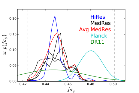
Next, we consider the effect of linearly varying the overall amplitude of the peculiar velocity field with the parameter , and interpret the result as a change in the effective . We justify this interpretation in Sec. 7.7. Here we consider only the case when the other velocity parameters and are held fixed. The marginalized distribution of shown in Fig. 16 is clearly noisy due to the finite volume of our -body simulation boxes. We therefore computed constraints separately from three independent MedRes boxes (labelled Fiducial=MedRes0, MedRes1, and MedRes2 in Table 4) as well as with the single HiRes box we had available (top row, third column in the table). The marginalized constraints are consistent across the boxes, despite the shift in fiducial value between the box cosmologies. Averaging over the MedRes simulation boxes, we find , consistent with our recent large-scale analysis of DR11 (Samushia et al., 2013) which found for a CDM expansion history. Our raw statistical error is equal to Planck’s CDM prediction of ; the difference between the two independent measurements is , which we take to be reasonable agreement since we have not included a modeling systematics error budget. Despite the dominance of satellite galaxies on the observed anisotropies (Fig. 13), there is still ample information on the rate of structure growth on these smaller scales where the clustering signal is strong and well-measured, resulting in a factor of 2.5 reduction in uncertainty on compared with our DR11 large-scale RSD analysis. In Fig. 17 we show the theoretical prediction from the best fit model using the MedRes0 box. In this model and we have held and fixed. Compared to the best fit model with () in Fig. 14, the amplitude of on large scales provides a better fit to the data. These are the same scales dominating the Samushia et al. (2013) large-scale RSD measurement of ; the last bins overlap between the analyses. The best fit models as a function of have nearly identical behavior in the first three bins Mpc, and divide on larger scales, indicating that the constraint on is driven by the relative amplitudes of and . Fig. 17 also shows that even though the model was fit to Mpc) and , it provides a good fit to out to 25 Mpc ( for 18 bins), and correctly models scales below the fiber collision radius, so that is also fit ( for 20 bins).

7.6 Robustness of the constraint to model extensions
The basic redshift-independent HOD model we are using to fit the CMASS clustering assumes that the observed galaxies are a subsample of objects defined by those HOD parameters. We enforce only a broad prior on from the observed CMASS selection function . However, both intrinsic stochasticity in the stellar mass-halo mass relation and photometric errors in the imaging catalog will broaden the distribution of halo masses hosting the CMASS sample. In order to test our sensitivity to the allowed host halo mass scatter, we refit our measurements with the prior shifted to higher values: . The results of fits that fix or vary are labelled in Table 4 as “high .” This choice is similar to relaxing our assumption that in Eq. 17 approaches one at large halo masses. Indeed, we find that this region of HOD parameter space provides a better fit to the observed clustering (). There are small (expected) shifts in the HOD parameters with the higher prior; most importantly for our conclusions in this work, the constraint on shifts by only . If we completely remove the prior, the HOD is limited to as approaches 0, which is an unphysical limit of noisy target selection producing a precise mass cut in central galaxy host mass. Given our HOD parametrization, models with higher number density are unable to generate sufficiently large clustering. Even in this unrealistic case, the shifts upward compared to our fiducial value by only .
Both the color selection and photometric errors in the imaging used for target selection could result in halos where the central galaxy does not pass our target selection cuts, while one or more satellite galaxies in that halo do pass. To test the impact of such cases (labelled “cen/sat” test in Table 4), we consider the drastic case where 20% of centrals in massive halos are not CMASS selected galaxies, implemented in our model by simply multiplying by 0.8. In contrast to the rest of our analyses, in this test we do not require a central galaxy in order for a particular halo to host a satellite galaxy, thus lowering the contribution of “one-halo” central-satellite pairs at fixed HOD parameters. This model provides a much better fit than our fiducial HOD assumptions (). The satellite fraction is larger, in the model moves closer to the typical in the sample, and the satellite occupation distribution steepens. In future work we hope to explore such model extensions more generally in concert with a better understanding of the impact of photometric errors on targeting, as well as redshift evolution and intrinsic diversity in the CMASS galaxy population. Again, the important result for the present work is that a plausible extension of our halo occupation modeling can improve the fit, but the constraint on shifts only slightly.

Next we consider the impact of varying the galaxy intrahalo velocities through the parameters and defined in Sec. 6.3. Their impact on the observable is shown in Fig. 18, holding the HOD parameters fixed to the best fit values for and . Increasing the intrahalo velocity dispersion lowers the number of pairs at small separations, while changing shifts the peak position in . The impact of on extends out to much larger scales than , as expected because intrahalo satellite velocities have a broader dispersion than centrals. Changing has a distinct scale dependence in both and , which should be distinguishable from and .
We introduce the parameter to rescale the relative velocity between satellite galaxies and their host halos. This parameter is meant to absorb the effect of galaxy velocity bias as well as variations in the halo mass function due to cosmological parameter uncertainties. White Cohn, & Smit (2010) examine in detail the velocity structure of subhalos within group-scale halos at z=0.1, and suggest a theoretical uncertainty in velocity bias of (10%). Wu et al. (2013) used -body and hydrodynamical simulations to study the relationship between the galaxy and dark matter intrahalo velocity dispersion in halos of mass , i.e., well-matched to the typical satellite galaxy host halo mass according to our HOD model fits. They found that averaging over all cluster galaxies, , while averaging only over the five brightest satellites yielded a ratio of 0.868. The latter is likely more applicable to the massive galaxies comprising the CMASS sample. Rather than smoothly varying , we run separate MCMC chains at and ; this range incorporates the small velocity biases found in Wu et al. (2013). Alternatively, neglecting velocity bias, a per-cent variation in corresponds to a factor of 0.5-1.7 change in the host halo mass scale of satellite galaxies. The fifth and sixth bottom columns of Table 4 show the result of these fits; is strongly disfavored by our data (), but the best fit of under this assumption is still in good agreement with our fiducial case at the level. Our data shows a preference for , indicating that our fiducial model may not produce strong enough finger-of-god features. Again, allowing freedom in does not shift or weaken the constraing on .
Finally, we also introduce additional random velocity dispersion for central galaxies through the parameter (final bottom column of Table 4). The fiducial value is preferred by the data. Allowing as a free parameter shifts the 68% confidence region on lower by . We do note that preliminary tests using the HiRes box showed that when both and are free (and both take large values outside the range considered here), the best fit value of is more dramatically reduced. The statistical precision of our fiducial constraint certainly warrants a further assessment of our uncertainties of the velocity structure of CMASS-type galaxies relative to their host dark matter halos. Appendix B showed that the velocity of the halo center is not well-defined, but depends on the averaging scale. We have chosen a scale that roughly matches the size of the typical CMASS galaxy, but ideally the uncertainty associated with this choice (and the potential impact of baryonic effects) should be accounted for in future work.
7.7 Non-linear velocities, cosmology dependence and light-cone effects
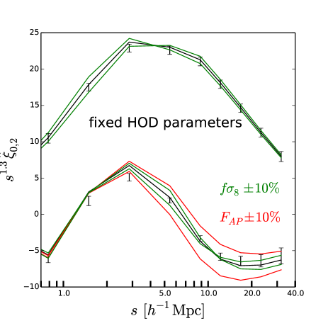
With the single exception of the cosmological parameter combination determining , we have not explored how our constraints depend on cosmological parameters. In this section we merely discuss where the largest sensitivities lie. Under the assumption of adiabatic fluctuations and the standard three species of massless neutrinos, the CMB observations tightly constrain the power spectrum of matter fluctuations (Planck Collaboration, 2013) with in units of Mpc; under these assumptions, depends only on physical densities and (see Section 5.1.1 of Reid et al., 2012). These tight constraints on the linear matter power spectrum should translate to strong constraints on the scale-dependence of halo clustering as well. As in other analyses simultaneously fitting cosmology and HOD-like parameters (Tinker et al., 2011; Cacciato et al., 2013; Mandelbaum et al., 2013), we naively expect most of our sensitivity to cosmological parameters to be through some combination of and .
We have allowed the overall amplitude of the halo peculiar velocity field in our simulations to vary, and in Sec. 7.5 have interpreted this amplitude as a constraint on . This linear scaling is expected to break down in the non-linear regime; recall, for instance, that perturbative corrections to the power spectrum are proportional to powers of the linear growth factor (, , …) times different functions of . To check the impact of both light cone effects and the scaling approximation, we examine halo catalogs from the MedRes0 box at neighboring redshift outputs: , for which . Thus the edges span a 10% change in the large-scale amplitude of matter fluctuations. We divide our fiducial halo catalog at into four mass bins split on the cumulative mass distribution from our best fit HOD model with boundaries edges at . Motivated by our observation in Appendix A that there is no measurable redshift evolution of the CMASS clustering, we shift these mass bins slightly at and , with the bin centers shifted to match the large scale value of in the original bins. The difference in the corresponding mass bin centers between the and outputs was at most 20%, for a 10% change in across this redshift range. Across this same redshift range, we measure the normalization of the relation to decrease by 7%. These two effects nearly cancel each other, so for HODs selecting halos with the same distribution of , the effective will remain at the-percent level, well within the range explored in the previous section. We expect small changes in other cosmological parameters to be within this prior as well. With these mass bins we can also compare the clustering and velocity statistics at different redshifts. By design, our bins have the large-scale clustering amplitude matched, so we can isolate the impact of non-linear growth on the underlying halo clustering. We first compare the matched real space correlation functions and pairwise infall velocities across redshift. Changes in non-linear growth to and at fixed large scale is not well-detected in this measurement using a single simulation box, but is constrained to be smaller than , except in the largest halo mass bin ( ), where the real and redshift-space monopoles change by and per-cent respectively below 1 Mpc in the expected directions. We detect no significant trends in . We conclude that at fixed cosmological parameters (other than ), non-linear corrections to the theoretical template can be neglected when inferring . Since the relevant halo clustering is so similar at the three redshifts, we infer that light-cone effects should have a negligible impact on our theoretical template. That is, our theoretical template from a fixed redshift output should be nearly the same as if we had generated it from a light cone (after perhaps small shifts in HOD parameters).
We have tested this assertion by refitting the measurements using the halo catalog from the MedRes box output at , where is 5% lower than at our fiducial . The matter clustering in this redshift slice should be closer to the clustering in a model with the overall amplitude of fluctuations lowered to match our best fit . However, the value of in the higher redshift slice is only smaller by 1% since increases with redshift. Accounting for this difference, we find , in excellent agreement with our fiducial fit using the halo catalog.
One additional impact of cosmological parameters is in the conversion of angles and redshifts into comoving coordinates. As in Anderson et al. (2013) and Samushia et al. (2013), we assume a cosmology with and for this conversion. We did not account for the difference between the fiducial cosmology and simulation cosmology in the theoretical model, but the error on the angle-averaged distance scale in Mpc units is only 1.0%. We checked that this error has a negligible impact on our theoretical predictions: the difference amounts to at fixed HOD parameters. The Alcock-Paczynski (Alcock & Paczynski, 1979) parameter distorts line-of-sight distances relative to transverse distances and at fixed , a change in alters while holding basically fixed. Fig. 19 compares the impact of 10% changes in and on at fixed HOD parameters; changes caused by the two parameters are distinguishable because of their differing scale dependence. Allowing uncertainty in will however degrade our constraints on ; in Reid et al. (2012) and Samushia et al. (2013) we report joint constraints on -. Since geometric parameters are “slow” variables in our theoretical calculation (they alter the separation between halo pairs), we defer a joint constraint to future work. Note that non-cosmological constant dark energy affects both geometric and growth of structure parameters, so our measurement of cannot be used to constrain dark energy without accounting for this degeneracy. The current work can be considered only a consistency test of the CDM + general relativity model, where is constrained to within 0.6% (Planck Collaboration, 2013). At fixed cosmological and HOD parameters in our model, varying by 1.2% produces a change in the theoretical prediction of , so we can safely neglect this uncertainty when testing models that assume a flat CDM expansion history.
7.8 Sensitivity of constraint to small scales
Finally, we assess the sensitivity of our constraint to the small-scale velocity distribution probed by by performing fits to Mpc) + Mpc) and Mpc) + Mpc); that is, the first (second) choice combines our fiducial measurements with the first five (last four) bins of our measurement. The first fit essentially recovers the results of our fiducial fit including all bins to nearly the same precision, implying that essentially all of our information comes from these non-linear scales and therefore potentially sensitively depends on the accuracy of our HOD modeling approach. Table 4 shows that for a reasonable range of extensions to our fiducial model, the constraint is stable.
The fit restricted to larger bins has considerable shifts in HOD parameters. While the satellite fraction is still well-constrained with the same central value, the distribution of the satellites shifts to lower halo masses. Rather than a constraint on , this fit prefers with 95% confidence, increases by 0.2, and . This HOD model has weaker FOG features, which therefore lowers to but also alters on small scales. The best fit to Mpc) + Mpc) is strongly disfavored using our fiducial set of measurements ().
7.9 Predicting
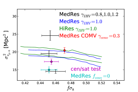
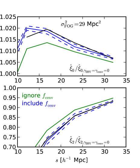
In Reid et al. (2012) and Samushia et al. (2013), we analysed the large scale with an analytic Gaussian streaming model to constrain along with geometric parameters and . The model has a single parameter, , to account for the effect of small-scale motions, like satellite galaxies within their host halos (traditional “fingers-of-god”). The model convolves the predicted halo auto-correlation function with a Gaussian, approximating the velocities of galaxies relative to their host halos as uncorrelated with the quasilinear flows of interest. We can estimate the probability distribution function of those velocities, assuming the central galaxies also have some residual motion specified by a fraction of the halo virial velocity. Using the halo model and assuming a central is required for a halo to host a satellite, we can estimate the probability distribution of galaxy velocities relative to their host halos as
| (20) |
where is a Gaussian probability distribution with variance and mean 0, and is the halo mass function. To get the pairwise velocity distribution component due to galaxy motions relative to the center-of-mass velocity of their host halos for pairs in different host halos, we convolve Eq. 20 with itself. The result has a narrow distribution about from central galaxy pairs, and an exponential tail due to the much larger satellite galaxy velocities. We can evaluate the second moment of this distribution, , at each point in our chains to determine its mean and uncertainty. 68% confidence intervals are shown in Fig. 20 as a function of for both the HiRes (green) and MedRes (blue) simulations over a broader range of values than is preferred by our fiducial MedRes fits (central black point, with 68% confidence in also shown). The plot shows that is very well constrained by our measurements and has only a modest degeneracy with . Varying the satellite galaxy relative velocities by by (upper and lower black points) also changes by 25%; note from Table 4 that provides a poor fit to our measurements of . Also shown in red is the constraint derived from a MedRes chain adopting center-of-mass velocities for central galaxies, but adding a random dispersion to central galaxies of magnitude and holding fixed. The “cen/sat test” model (magenta point) described in Sec. 7.6 relaxes the assumption that halos hosting satellite CMASS galaxies also always host centrals; this model produces a similar value of as our fiducial one. Finally, we can also separate the contributions from central and satellites to the dispersion in Eq. 20. In our default chain, we find the central term to contribute and the satellite term to contribute (shown in cyan on the figure). It is therefore imperative to allow for some dispersion in both the central and satellite galaxies, relative to the bulk halo motion. To incorporate a reasonable uncertainty on and , we suggest a conservative Gaussian prior on centered at 19.5 Mpc2 and with uncertainty of Mpc2 to account both for uncertainty corresponding to uncertain by 20% and central galaxy dispersion uncertain at the 100% level.
Before we can apply this prior to our analysis of large scale clustering, we need to understand the relation between the nuisance parameter and , which we estimate from the HOD constraints from small scale clustering; the relation is non-trivial due to the non-Gaussianity of . Unfortunately, constraints on by fitting mock catalogs directly with cosmoxi2d (the theoretical prediction software used in Reid et al. 2012 and Samushia et al. 2013) on the same large scales as the data is extremely noisy, even at known and geometric parameters. We remove much of the cosmic variance in the inference of from mock catalogs by considering the ratios . In particular, we assign center-of-mass halo velocities to the central galaxies to compute the denominator but use in the numerator, since we found the first term in Eq. 20 is not negligible, and the majority of perturbation theory models (including cosmoxi2d) are validated using halo catalogs containing . The resulting ratio is shown in blue in Fig. 21 for the MedRes box. A 68% error band shown as blue dashed curves are derived from the uncertainty on the HOD parameters using the default chain with , , and free; comparison with two additional MedRes boxes indicates that cosmic variance is a subdominant contribution to the uncertainty for the ratio.
We compute an analogous ratio using cosmoxi2d, varying in the numerator and setting it to 1 Mpc2 in the denominator, consistent with the expected value for halos reported in Reid & White (2011). cosmoxi2d is based on perturbation theory, and the underlying model for halo clustering breaks down at Mpc. We therefore determine the best fit using only the last bin in our small-scale measurements, 27-38 Mpc and find Mpc2. Fig. 21 shows that the scale-dependent distortions to caused by the relative velocities between halos and galaxies is described well by the nuisance parameter , even to smaller scales than included in the cosmoxi2d analysis. Experimenting with a few other cases, we find the mapping to be a good predictor for the best fit cosmoxi2d nuisance parameter. Thus we adopt a Gaussian prior on Mpc2 and recompute DR11 large scale constraints in the case assuming a CDM expansion history, where Samushia et al. (2013) originally found . With the new prior, the constraint shifts to . The modest reduction in the uncertainty is not surprising, since the original hard prior on (0-50 Mpc2) was only slightly broader than the new prior. The small shift in the central value comes from the new prior eliminating the lowest end of the originally allowed range of ; the small-scale clustering requires satellite galaxies, and thus non-zero . One important difference between the small-scale and large scale analyses is the use of FKP weights in the latter; we therefore verified that we recover very similar small-scale clustering when applying the FKP weights, so that our derived prior on remains valid for an FKP weighted correlation function used to analyse large scales.
8 Implications for modified gravity models
Substantial research efforts have recently been devoted to exploring modifications of gravity as a means to explain the apparent cosmic acceleration (Clifton et al., 2012). Schmidt, Vikhlinin, & Hu (2009) showed that for the model, constraints on non-linear scales, in this case from clusters, are times stronger than those obtained on quasi-linear scales. Recently, the velocity structure around massive halos on 1-30 Mpc scales has been identified as a promising observational probe of modified gravity models, both for models with the chameleon screening mechanism (Lam et al., 2012, 2013; Zu et al., 2013) and a galileon model with the Vainshtein screening mechanism (Zu et al., 2013). In both the and galileon models studied by Zu et al. (2013), the infall velocity around halos at was enhanced by on scales of 5 Mpc, the real space halo-matter cross-correlation function showed a scale-dependent enhancement, peaking at at 2 Mpc, and velocity dispersions increased as well. All three effects would propagate to our observable, and we would expect modifications of the same order. Lam et al. (2012, 2013) frame this gravity test in combination with weak lensing, used to measure the mass of the central halos; Zu et al. (2013) showed that similar deviations persist in abundance matched samples of halos. While we plan to incorporate galaxy-galaxy lensing constraints on halo masses in future work (Leauthaud et al., prep), one can still search for the signatures of modified gravity using our measurements, but comparing to clustering-amplitude matched halo samples. The overall amplitude of galaxy clustering observed in our sample constrains the product of the mean halo bias (determined by the galaxy HOD) and the amplitude of matter fluctuations at the effective redshift of the galaxy sample, . Thus, for a given modified gravity model (realized with an -body simulation), the HOD would be constrained by the same procedure as we have implemented here for the case of general relativity. With the overall amplitude of clustering matched on Mpc scales, the modifications to the pairwise infall velocities and dispersions will propagate to scale-dependent changes in our observables. While we are unable to provide any quantitative constraints without halo catalogs derived from modified gravity simulations, the precision of our GR-based constraint should severely limit the types of modifications described above.
9 Conclusions and Future Prospects
We have made the most precise comparison to date between the observed anisotropic clustering of galaxies at relatively small separations ( Mpc) and the predictions of a standard halo model in the context of CDM. We found good agreement between our simplified, redshift-independent HOD model and our measurements of both the projected and anistropic clustering on small scales. Our fits constrain the growth rate of cosmic structure at the effective redshift of our galaxy sample: . This constraint is consistent with but improves on our DR11 analysis of large scale anistropy (Samushia et al., 2013) by a factor of 2.5. Intriguingly, our result has the same statistical power but is low compared with Planck’s CDM prediction, (Planck Collaboration, 2013).
The competitive statistical precision of our measurement warrants a systematic evaluation of the observational and modeling systematics. For the former, we introduced a new anisotropic clustering statistic that does not include information below the fiber collision scale, but approaches the usual multipoles on large scales. We carefully assessed the systematic and observational uncertainties from the angular upweighting method to correct fiber collisions to order to estimate the projected correlation function . We combined these measurements to obtain robust joint constraints on the halo occupation distribution and growth rate of cosmic structure probed by CMASS galaxies.
To assess the robustness of our modeling assumptions, we investigated several generalizations to our HOD assumptions and particularly how we assign velocities to the mock galaxies from which we draw our theoretical predictions; the results are summarized in Table 4. The variations we examined caused at most shifts in the constraints. However, given the statistical precison of our reported constraint, further investigation with more sophisicated modeling of the galaxy-halo connection is warranted. Of the possibilities we explored, a model that relaxes the assumption that halos hosting satellite galaxies also host centrals (labelled “cen/sat test”) improved the fit to our measurements by but did not shift constraints appreciably. Such a model is well-motivated by our target selection process – both color cuts and photometric errors cause massive galaxies to scatter in and out of the sample. Alternatively, we can also improve the model fit by increasing the satellite galaxy velocity dispersion at fixed halo mass.
At least within the cosmological parameter space we explored, we found that for two different definitions of the central galaxy velocity, the data prefer , the motion of the densest clump, over , the halo center-of-mass velocity averaged over all particles within . A comparison of these two velocity fields also indicates a possible shift of in the effective large scale , and should therefore be considered when this level of precision is reached.
While we have not tested any explicit modified gravity models, we have shown that the clustering of few Mpc halos are consistent with the expectations of CDM and a simple picture of galaxy formation in which halo mass is the only relevant variable determining the probability of hosting a CMASS galaxy. To quantify the precision of this test, our best fit model matches the observed at the 3 per-cent level from 0.8 - 32 Mpc, and 15 to 5 per-cent level from 5 to 32 Mpc for , with reasonable agreement compared to our uncertainties on smaller scales as well.
As the example of shows, modified gravity could potentially dramatically alter structure growth on these scales, and our analysis should be used to constrain such models. In addition to the constraint afforded by our measurements, more precise galaxy velocity bias predictions in CDM would allow our joint constraints on and to be interpreted as an additional consistency test between the halo mass inferred from clustering amplitude , and from the halo virial velocities probed by .
Finally, even ignoring the information of the small-scale clustering on , our data tightly constrain the impact of the intra-halo motions of galaxies on clustering at relatively large scales. We derive a prior on the “finger-of-god” nuisance parameter that is tighter but consistent with the prior adopted in Reid et al. (2012) and Samushia et al. (2013). Moreover, our detailed study of the clustering on small scales also allowed us to validate that as defined in those works can precisely describe the impact of intra-halo velocities of CMASS galaxies on quasi-linear scales.
10 Acknowledgements
We thank Cameron McBride for help in creating the tiled mock, as well as Zheng Zheng, Hong Guo, and the anonymous referee for useful discussions/suggestions.
Funding for SDSS-III has been provided by the Alfred P. Sloan Foundation, the Participating Institutions, the National Science Foundation, and the U.S. Department of Energy Office of Science. The SDSS-III web site is http://www.sdss3.org/.
SDSS-III is managed by the Astrophysical Research Consortium for the Participating Institutions of the SDSS-III Collaboration including the University of Arizona, the Brazilian Participation Group, Brookhaven National Laboratory, University of Cambridge, Carnegie Mellon University, University of Florida, the French Participation Group, the German Participation Group, Harvard University, the Instituto de Astrofisica de Canarias, the Michigan State/Notre Dame/JINA Participation Group, Johns Hopkins University, Lawrence Berkeley National Laboratory, Max Planck Institute for Astrophysics, Max Planck Institute for Extraterrestrial Physics, New Mexico State University, New York University, Ohio State University, Pennsylvania State University, University of Portsmouth, Princeton University, the Spanish Participation Group, University of Tokyo, University of Utah, Vanderbilt University, University of Virginia, University of Washington, and Yale University.
The simulations used in this paper were analysed at the National Energy Research Scientific Computing Center, the Shared Research Computing Services Pilot of the University of California and the Laboratory Research Computing project at Lawrence Berkeley National Laboratory.
BAR gratefully acknowledges support provided by NASA through Hubble Fellowship grant 51280 awarded by the Space Telescope Science Institute, which is operated by the Association of Universities for Research in Astronomy, Inc., for NASA, under contract NAS 5-26555.
This work was supported in part by the National Science Foundation under Grant No. PHYS-1066293 and the hospitality of the Aspen Center for Physics.
AL was supported by the World Premier International Research Center Initiative (WPI Initiative), MEXT, Japan.
Appendix A Redshift evolution of
Throughout this analysis we have treated the CMASS sample within as a single population. One reason for this is that fiber collision corrections using the angular upweighting become substantially more uncertain as the spectrosopic sample becomes a smaller subset of the target sample. However, the nearest neighbor correction method should be valid in arbitrary redshift bins. Fig. 22 shows our measurement of using the nearest neighbor redshift correction for redshift cuts that split the sample equally into three bins in both the north and south. These bins also have different galaxy weighted number densities: 3.4, 3.4, and 1.5 . Rescaling the bootstrap covariance matrix derived for the full sample by to compute an approximate difference between the subsamples and the full sample, we find these subsample clustering measurements to be consistent with being drawn from the full sample (), with the exception of the highest redshift bin in the north ( for 18 bins); comparison with the same bin in the south suggests most of the difference could be cosmic variance rather than a systematic change from the clustering of the full sample. The covariance matrix used for this comparison is approximate and does not include any of our theoretical error budget. Remarkably, our target selection algorithm selects galaxies with very similar clustering across the redshift range of our sample, even though the linear growth factor increases by 14% in our fiducial cosmology between and .
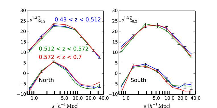
Appendix B Sensitivity to the halo central velocity definition
Using the MedRes simulation box, we explore in the left panel of Fig. 23 the mean square velocity difference between the halo center of mass velocity and various central velocity definitions, in units of the halo velocity dispersion: the velocity of the particle at the potential minimum (red), the velocity averaged over the innermost 10 and 20 particles (green), the velocity averaged over a fixed fraction of the innermost halo members, ranging from 3.75% to 40% (blue), and the fiducial choice adopted in this work (thick black dashed line) and detailed in Sec. 2.4. The right panel demonstrates that the mean square dispersion of the central velocity depends on the fraction of innermost halo particles used to determine the central velocity (blue curve). For uncorrelated intrahalo motions, we would expect the green curve; we interpret the difference (red curve) as evidence for bulk motion of the central galaxy. This naive noise estimate suggests that our fiducial central velocity definition has a sizeable contribution from particle noise. We integrate the square velocity difference in the central velocity dispersion between our MedRes and HiRes simulations (lower dashed and solid curves in Fig. 10) over the best fit HOD, and find only a 13% excess in the MedRes simulation. Since the HiRes mass resolution is eight times larger, we are therefore confident that our central galaxy velocities are negligibly affected by resolution in the mass range of interest for this analysis.
However, since their is no apparent convergence of the central velocity dispersion at small smoothing scales, we expect our predictions for galaxy clustering to be sensitive to this choice. In Sec. 2.4 we argued that our fiducial choice corresponds to the typical galaxy size for the population we are modeling, at least over the halo mass range that dominates the clustering signal. Moreover, our fiducial choice provides approximately the correct amount of central velocity dispersion to match the observed ; slight modifications to the central velocity definition may improve the fit on small scales. We have not explored this possibility further here, but hope to in future work. We note that the final test in Sec. 7.6 showed that our measurements do not favor additional random central velocity dispersion. Examination of hydrodynamic galaxy formation simulations would shed light on both the impact of baryonic effects and could determine the best algorithm to estimate the central galaxy velocity from dark matter-only simulations.
Finally, we note that a similar effect was discussed in Behroozi, Wechsler, & Wu (2013); their Figure 11 includes the median three-dimensional velocity offset at in halo mass bins, but averaged in spherical shells rather than including all particles within a given radius. Nonetheless, from their plots we would expect km for and halos, averaged over 0.06 (0.12) Mpc, while our measurements shown in Fig. 10 predicts 110 (237) km for the rms three-dimensional rms velocity at this redshift. In addition, we find the one-dimensional velocity distribution of to be approximately exponential, for which we expect the rms to be larger than the median by a factor of . Therefore the amplitude of the bulk velocities in this work seems consistent with that found in Behroozi, Wechsler, & Wu (2013) using the ROCKSTAR halo finder with slightly higher mass resolution.
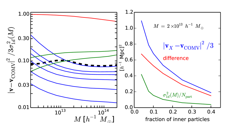
References
- Planck Collaboration (2013) Ade P. et al., 2013, arXiv:1303.5076
- Ahn et al. (2013) Ahn C., et al., 2014, ApJS, 211, 17
- Aihara et al. (2011) Aihara H., et al., 2011, ApJS, 193, 29
- Alcock & Paczynski (1979) Alcock C., Paczynski B., 1979, Nature, 281, 358
- Anderson et al. (2013) Anderson L., et al., 2013, arXiv:1312.4877
- Behroozi, Wechsler, & Wu (2013) Behroozi P., Wechsler R., Wu H., 2013, ApJ, 762, 109
- Benson et al. (2000) Benson A., Cole S., Frenk C., Baugh C., Lacey C., 2000, MNRAS, 311, 793
- Berlind & Weinberg (2002) Berlind A., Weinberg D., 2002, ApJ, 575, 587
- Beutler et al. (2013) Beutler F., et al., 2013, arXiv:1312.4611
- Blanton et al. (2003) Blanton M., et al., 2003, AJ, 125, 2276
- Bolton et al. (2012) Bolton A., et al., 2012, AJ, 144, 144
- Cacciato et al. (2013) Cacciato M., van den Bosch F., More S., Mo H., Yang X., 2013, MNRAS, 340, 767
- Chuang et al. (2013) Chuang et al., 2013, arXiv:1312.4889
- Clifton et al. (2012) Clifton T., Ferreira P., Padilla A., Skordis C., 2012, Physics Reports, 513, 1
- Cohn & White (2013) Cohn J., White M., 2013, arXiv:1311.0850
- Conroy, Wechsler, & Kravtsov (2006) Conroy C., Wechsler R., Kravtsov A., 2006, ApJ, 647, 201
- Cooray & Sheth (2002) Cooray A., Sheth R., 2002 Physics Reports, 372, 1
- Davis et al. (1985) Davis M., Efstathiou G., Frenk C., White S., 1985, ApJ, 292, 371
- Dawson et al. (2012) Dawson K., et al., 2013, AJ, 145, 10
- de la Torre et al. (2013) de al Torre S., 2013, A&A, 557, 54
- Eifler, Kilbinger, & Schneider (2008) Eifler T., Kilbinger M., Schneider P., 2008, A&A, 482, 9
- Eisenstein et al. (2011) Eisenstein D.J., et al., 2011, AJ, 142, 72
- Fisher (1995) Fisher K.B., 1995, ApJ, 448, 494
- Gao et al. (2005) Gao L., Springel V., White S., 2005, MNRAS, 363, 66
- Gunn et al. (1998) Gunn J.E., et al., 1998, AJ, 116, 3040
- Gunn et al. (2006) Gunn J.E., et al., 2006, AJ, 131, 2332
- Guo et al. (2014) Guo H., et al., 2014, arXiv:1401.3009
- Guo, Zehavi, & Zheng (2012) Guo H., Zehavi I., Zheng Z., 2012, ApJ, 756, 127
- Hartlap, Simon & Schneider (2007) Hartlap J., Simon P., Schneider P., 2007, A&A,464,399
- Hawkins et al. (2003) Hawkins E., et al., 2003, MNRAS, 346, 78
- Hikage (2014) Hikage C., 2014, arXiv:1401.1246
- Kaiser (1987) Kaiser N., 1987, MNRAS, 227, 1
- Keisler (2013) Keisler R., Schmidt F., 2013, ApJ, 765, 32
- Komatsu et al. (2011) Komatsu E., et al., 2011, ApJS, 192, 18
- Jackson (1972) Jackson J., 1972, MNRAS, 156, 1P
- Krause et al. (2013) Krause E., 2013, MNRAS, 428, 2548
- Lam et al. (2012) Lam T., Nishimichi T., Schmidt F., Takada M., 2012, PhRvL, 109, 1301
- Lam et al. (2013) Lam T., Schmidt F., Nishimichi T., Takada M., 2013, PhRvD, 88, 023012
- Landy & Szalay (1993) Landy S.D., Szalay A.S., 1993, ApJ 412, 64
- Leauthaud et al. (prep) Leauthaud A., et al., in prep.
- Limber (1954) Limber D., 1954, ApJ, 119, 655
- Li et al. (2006) Li C., Kauffmann G., Jing Y., White S., B’́orner G., Cheng F., 2006, MNRAS, 368, 21
- Mandelbaum et al. (2013) Mandelbaum R., Slosar A., Baldauf T., Seljak U., Hirata C., Nakajima R., Reyes R., Smith R., 2013, MNRAS, 432, 1544
- Marin (2011) Marin F., et al., 2011, ApJ, 737, 97
- Marinoni & Hudson (2002) Marinoni C., Hudson M., 2002, ApJ, 569, 101
- Masters et al. (2011) Masters K. et al., 2011, MNRAS, 418, 1055
- Neistein & Khochfar (2012) Neistein E., Khochfar S., 2012, arXiv:1209.0463
- Norberg et al. (2009) Norberg P., Baugh C., Gaztañaga E., Croton D., 2009, MNRAS, 396, 19
- Nuza et al. (2013) Nuza et al., 2013, MNRAS, 432, 743
- Parejko et al. (2013) Parejko J., et al., 2013, MNRAS, 429, 98
- Peacock & Smith (2000) Peacock J., Smith R., 2000, MNRAS, 318, 1144
- Piloyan et al. (2014) Piloyan A., Marra V., Baldi M., Amendola L., arXiv:1401.2656
- Reid et al. (2012) Reid B., et al., 2012, MNRAS, 426, 2719
- Reid & Spergel (2009) Reid B., Spergel D., 2009, ApJ, 702, 249
- Reid & White (2011) Reid B., White M., 2011, MNRAS, 417, 1913
- Reyes (2010) Reyes R., 2010, Nature, 464, 256
- Ross et al. (2012) Ross A. et al., 2012, MNRAS, 424, 564
- Ross et al. (2014) Ross A. et al., 2014, MNRAS, 437, 1109
- Ross et al. (2007) Ross N., et al., 2007, MNRAS, 381, 573
- Samushia et al. (2013) Samushia L., et al., 2013, arXiv:1312.4899
- Sanchez et al. (2013) Sanchez A., et al., 2013, arXiv:1312.4854
- Schmidt, Vikhlinin, & Hu (2009) Schmidt F., Vikhlinin A., Hu W., 2009, PhRvD, 80, 083505
- Sheth (2005) Sheth R., 2005, MNRAS, 364, 796
- Seljak (2000) Seljak U., 2000 MNRAS, 318, 203
- Seo, Eisenstein, & Zehavi (2008) Seo H. J., Eisenstein D., Zehavi I., 2008, ApJ, 681, 998
- Tinker (2007) Tinker J., 2007, MNRAS 374, 477
- Tinker et al. (2011) Tinker J. et al., 2012, ApJ, 745, 16
- Tinker et al. (2008) Tinker J., Kravtsov A., Klypin A., Abazajian K., Warren M., Yepes G., Gottl’́ober S., Holz D., 2008, ApJ, 688, 709
- Tinker et al. (2010) Tinker J., Robertson B., Kravtsov A., Klypin A., Warren M., Yepes G., Gottl’́ober S., 2010, ApJ, 724, 878
- White et al. (2011) White M., et al., 2011, ApJ, 728, 126
- White Cohn, & Smit (2010) White M., Cohn J., Smit R., 2010, MNRAS, 408, 1818
- White, Hernquist, & Springel (2001) White M., Hernquist L., Springel V., 2001, ApJ, 550, 129
- White & Padmanabhan (2009) White M., Padmanabhan N., 2009, MNRAS, 395, 2381
- Vale & Ostriker (2006) Vale A., Ostriker J., 2006, MNRAS, 371, 1173
- van den Bosch et al. (2013) van den Bosch F., More S., Cacciato M., Mo H., Yang X., 2013, MNRAS, 430, 725
- van den Bosch et al. (2005) van den Bosch F., Weinmann S., Yang X., Mo H., Li C., Jing Y., 2005, MNRAS, 361, 1203
- Wang et al. (2013) Wang L., Weinmann S., De Lucia G., Yang X., 2013, MNRAS, 433, 515
- Wu et al. (2013) Wu H., Hahn O., Evrard A., Wechsler R., Dolag K., 2013, MNRAS, 436, 460
- Yang et al. (2004) Yang X., Mo H., Jing Y., van den Bosch F., 2004, MNRAS, 350, 1153
- Yang, Mo, & van den Bosch (2003) Yang X., Mo H., van den Bosch F., MNRAS, 339, 1057
- Yang, Mo, & van den Bosch (2009) Yang X., Mo H., van den Bosch F., 2009, ApJ, 695, 900
- York et al. (2000) York D.G., et al., 2000, AJ, 120, 1579
- Zehavi et al. (2011) Zehavi I. et al., 2011, ApJ, 736, 59
- Zentner, Hearin, van den Bosch (2013) Zentner A., Hearin A., van den Bosch F., 2013, arXiv:1311.1818
- Zheng et al. (2005) Zheng Z., et al., 2005, ApJ, 633, 791
- Zu et al. (2013) Zu Y., Weinberg D., Jennings E., Baojiu L., Wyman M., 2013, arXiv:1310.6768
- Zu & Weinberg (2012) Zu Y., Weinberg D., 2013, MNRAS, 431, 3319