Long-range correlations and trends in Colombian seismic time series
Abstract
We study long-range correlations and trends in time series extracted from the data of seismic events occurred from 1973 to 2011 in a rectangular region that contains mainly all the continental part of Colombia. The long-range correlations are detected by the calculation of the Hurst exponents for the time series of interevent intervals, separation distances, depth differences and magnitude differences. By using a modification of the classical method that has been developed to detect short-range correlations in time series, we find the existence of persistence for all the time series considered except for magnitude differences. We find also, by using the until the third order, that the studied time series are not influenced by trends. Additionally, an analysis of the Hurst exponent as a function of the number of events in the time and the maximum window size is presented.
1 Introduction
Among the properties that time series of different kind of phenomena exhibit, one of the most interesting is the long-range correlation [1]. This correlation, also known as long memory or long-range persistence, means that the autocovariance function decays exponentially, by a spectral density that tends to infinity [2, 3]. However, at the critical point, the exponential decay turns into a power-law decay [2, 4]. Long-range power-law correlations can be observed in a very wide range of systems, as for instance in smoke-particle aggregates [5], nucleotide sequences [6], earthquake processes [7], mosaic structure of DNA [8], literary texts [9], stride interval of human gait [10], cardiac interbeat intervals [11], stock index variations [12], sedimentation [13], variations of daily maximum temperatures [14], neuron activity [15], stratus cloud liquid water [16], stock returns [3], electric signals [4], seismic sequences [17, 18], and relativistic nuclear colisions [19].
Some geophysical processes are characterized by self-similarity correlations because the dynamics are based on the interaction of many components over a wide range of time or space scales [20]. An example of complex systems in geophysics are earthquakes, characterized by power-law distributions of spatial, temporal and energy parameters [21]. The complex phenomenology exhibited by earthquakes is due to the deformation and sudden rupture of parts of the earth’s crust because of the external forces acting from plate tectonic motions [22].
Long-range power-law correlations are traditionally measured by a scaling parameter or fractal dimension . If the time series is self-similar and self-affine, the parameter is related to the Hurst exponent () through the expression [23, 24]. Thus, the Hurst exponent is a measure of the long-range correlation in time series data and allows to distinguish the persistence (correlation), anti-persistence (anti-correlation) or randomness of the data [25]. The original estimation of the Hurst exponent was first performed in hydrology by Harold Edwin Hurst in 1951 [26], by introducing an empirical relationship called the Rescaled-Range . Posteriorly, this relationship became the start point to establish the Classical () method developed by Mandelbrot and Wallis into the context of the fractal geometry [25, 27, 28].
Although the is one of the most popular methods to calculate the Hurst exponent, it has shown some serious limitations to study long-range correlation when the time series is not large enough [29, 30]. However, a possible solution of this problem was proposed by W. Lo, which we call the Modified R/S method [31]. Another of the most popular methods to calculate de Hurst exponent is the Detendred Fluctuation Analysis proposed by Peng et al. [8]. One of the main advantages of the is that it can remove trends present in some real time series [32, 33, 34]. Additionally, this method can be generalized for the multifractal characterization of nonstationary time series [35].
The study of long-range power-law correlations in seismic sequences has been focussed on the calculation of the Hurst exponent for time series of interevent intervals by using the [24] and the [17, 18]. The DFA was also used to calculate the Hurst exponent associated to two-dimensional sequences defined in terms of the time series of interevent intervals and separation distances [36]. Furthermore, other time series like temporal and spatial variations were studied using the method [37]. Persistence in temporal sequences for earthquake activity has been recognized and reported in a number of studies [17, 18, 24, 37] and also for the temporal-spatial sequences [36]. This result is consistent with the fractal structures in time, space, and magnitude dimensions observed in the seismicity of earthquakes [38, 39, 40]. However, most recently, an anti-correlated behaviour of the earthquake magnitude time series was observed from the calculation of the Hurst exponent using the [41]
Until now the calculation of the Hurst exponent in seismic time series has been focussed in temporal, temporal-spatial and magnitude sequences [17, 18, 24, 36, 37, 41]. In this work we extend the detection of long-range correlations for the case of new time series that can be extracted from the seismic event data. Additionally to the time series of interevent intervals [17, 18, 24, 37, 43], we consider also the time series associated to the following parameters defined between two successive seismic events: separation distance [38, 36]; depth difference; magnitude difference. We think that if we study simultaneously the existence of long-range correlations for these four seismic time series, then we have a most complete vision of the fractal structure associated to the seismic events [38]. Because the interaction between a previous event and the event caused by it relaxes with the time, it is possible to observe simultaneously a self-similar structure in time, space and magnitude distributions of the seismic event epicentres [38, 39, 40].
The main goal of this work is to detect whether long-range correlations and trends exist in time series extracted from the data of seismic events that occurred since 1973 until 2011 in a rectangular region that contains mainly all the continental part of Colombia. During this lapse of 39 years, the region under study, which contains also parts of Brazil, Ecuador, Panama, Peru and Venezuela, presented a total of 3932 seismic events with magnitudes higher than 4 according to the U.S. Geological Survey data base [42]. To detect the existence of long-range correlations in the time series of interevent intervals, separation distances, depth differences and magnitude differences, we calculate the Hurst exponents associated to these time series by using the method [31]. To appreciate the advantage of using the method, we first calculate the Hurst exponents for all the time series by using the method. With the purpose to eliminate trends in the seismic time series considered here, we calculate the Hurst exponents using the until the third order [32, 33, 35].
The reason why we use the [31] is because the might lead to an overestimation of the Hurst exponent, specially if seismic time series are constructed with less than 5000 data points as happened in this work. On the other hand, a study previously performed using data of Southern México [37] has detected the existence of cycles in the interevent interval sequence and this fact has been considered as a sign of trends in the associated seismic time series. For this reason, in this work, we use also the with the purpose to find polynomial trends on the data. We study also the evolution on time of the correlation between the Hurst exponent and the magnitude for the interevent interval in the seismological active area of the subduction zone of the Nazca and the South American plates in Colombia. The goal of this part of our study is to analyse if there is a statistical correlation between the value of the Hurst exponent and the magnitude of the seismic event, as it was found for the time series of interevent intervals in Southern México [37]. For accurateness, a study on the maximum window size in the calculation of the Hurst exponent is also performed, focusing the interest on the Hurst exponent as a function of the number of events in the time and the maximum window size.
2 Methods to calculate the Hurst exponent
2.1 Classical Rescaled Range (CR/S)
The method allows to study the long-range dependence for non-stationary time series by means of the calculation of the Hurst exponent [25, 27, 28]. Specifically, a value corresponds to anti-correlated data (anti-persistence behaviour), a value corresponds to correlated data (persistence behaviour) and the value corresponds to random data (uncorrelated behaviour) [25]. The definition of can be extended to values larger than [43]. In this way, the case corresponds to Brownian motion, the case correspond to brown noise and the case corresponds to black noise [43].
In the method the time series under consideration
is composed by
values. The full time series is divided into windows of size
. The number of windows is defined by
and therefore there are
windows of data , with
.
Defining the vector , the average over each window is
calculated as
| (1) |
The profile or sequence of partial summations , with , is defined as the cumulative summation minus the average of the corresponding window
| (2) |
The range of the window is defined as the maximum minus the minimum data point of the profile
| (3) |
The standard deviation of each window is given as
| (4) |
The rescaled range is described by the quantity , which is defined as
| (5) |
For the case in which a stochastic process associated to the data sequence under study is rescaled over a certain domain , the statistics follows the power law
| (6) |
Herein, is a constant and is the Hurst exponent which represents a fractal measure of the long-range correlations in the analysed data.
2.2 Modified Rescaled Range (MR/S)
When dealing with short time series (of less than 5000 values), the method looses precision [29]. In order to study short time series the R/S statistics should be modified so that it accounts for short memory processes [31]. When the time series under consideration is subject of short-range dependence, the variance should also include the auto-variances. This is accomplished when the standard deviation term described in equation (4) is replaced by the term:
| (7) |
where is the sample variance and the sample autocovariance. The parameter represents the lags in the weighted autocovariances.
2.3 Detrended Fluctuation Analysis (DFA)
An important tool to leave out trends in time series is the [32, 33, 34]. Trends can affect the time series and make them seem to be persistent when there is not a real correlation between the data points [32, 33, 34]. In order to find the correct scaling behaviour of the series, such trends have to be well distinguished. It is not easy to identify the origin of trends, so very often we do not know the reasons for underlying trends in collected data and we do not know the scales of underlying trends. DFA is a method for determining the scaling behaviour of data in the presence of possible trends without knowing their origin and shape [21]. In the following, the method to calculate the Hurst exponent via is explained.
As the first step of the , it is necessary to
calculate the profile or cumulative summations minus the average
of all the data
| (8) |
where runs over each data point .
As a second step, the profile is divided into windows of size and a fit of order of the window is subtracted from each data point. Choosing the order to be , each new data point is described as
| (9) |
where and are respectively the slope and the intercept of the linear fit done over the window . For this case, the subscript runs over the windows . The fluctuation is calculated as
| (10) |
Varying the size of the window and
consequently the number of windows , the Hurst
exponent corresponds to the slope in the
log-log plot of . If a stochastic process is
associated to the data sequence under study, it will follow the power
law
| (11) |
Different hierarchies of methods are employed for the fluctuation
analysis. Those hierarchies differ from each other in how the
fluctuations are measured and how trends are eliminated. By
definition eliminates trends of order
in the original time series and
in the profile
[32, 33, 34]. For instance,
corresponds to the simplest type of
fluctuation analysis and in this case the trends are not
eliminated. In the first order detrended fluctuation analysis
, the variance of the profile in each window
represents the square of the fluctuations and then the best linear
fit is determinated [34].
3 Data acquisition
We consider in this work the time series associated to the following parameters defined between two successive seismic events: (i) interevent interval [17, 18, 24, 37, 43]; (ii) separation distance [38, 36]; (iii) depth difference; (iv) magnitude difference. We note that the seismic time series of depth differences and magnitude differences are new for this kind of analysis. The analysis for time series of separation is new because we consider the time series of separation distances as independent respect to the time series of interevent intervals different from reference [36].
We analyzed the above mentioned time series because we are interested in knowing the scaling behavior of the most important characteristics of earthquakes. We think that knowing the behavior between, for example, the depth or the epicenter distance, or the difference in magnitude of two consecutive events in an area, would help to better describe the fractal behavior of the earthquakes.
The time series of separation distances is extracted from the seismic event data using the following definition for the angular distance in degrees between two events [38, 36]
| (12) |
where and are respectively the colatitudes and the longitudes of the two events [38, 36]. If we multiply the angular distance by 111 km, then we obtain the separation distance between two successive seismic events [36].
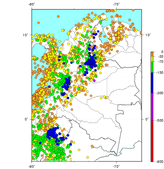
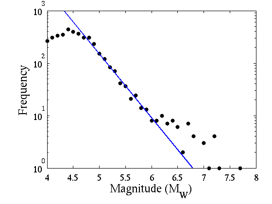
The time series of interevent intervals, separation distances, depth differences and magnitude differences are constructed from the seismic event data that we have obtained from the free online database of the United States Geological Survey [42]. A rectangular region that contains mainly all the continental area of Colombia was chosen to analyse the seismic data occurred from 1973 to 2011. As it is possible to observe in Figure 1, this region also contains parts of Brazil, Ecuador, Panama, Peru and Venezuela. Seismic events with magnitudes higher than 4 were selected in such a way that the total number of events initially considered was 3932. Using these data, Figure 2 presents the plot of the logarithm of the frequency as a function of the magnitude of the seismic event. The blue line in Figure 2 underlines the events with magnitudes from 4.8 to 6 that correspond to the ones that satisfy the Gutenberg-Richter law. Those events define the set that is used to perform the Hurst exponential analysis that will be presented below. It is important to mention that this methodology based on the Gutenberg-Richter law has been widely used in this kind of analysis [17, 18, 36, 24, 37].
4 Persistence and trends in Colombian seismic data
Long-range correlations for temporal and temporal-spatial sequences have been detected previously by the calculation of Hurst exponent for different seismic active areas of the world, as for instance of Italy [17, 18], USA [36, 41, 43], Taiwan [24], México [37], and Greece [44]. In this section we present the results of the calculation of the Hurst exponent for the Colombian seismic time series of interevent intervals, separation distances, depth differences and magnitude differences. Firstly, we present the Hurst exponents that were calculated using both the and methods. By using the method, we obtain Hurst exponents more precise, correcting for the effect of insufficiency of data (less than 5000 data points). Secondly, we present the Hurst exponents calculated using the until the third order. In this way, we can remove the trends which are present in the seismic time series under study.
4.1 Hurst exponents and scarcity effects
A correct degree of long-range correlation, represented by a precise calculation of the Hurst exponent, in time series composed by a relative small quantity of data can not obtained by using the method.
We have tested 1000 random time series of 100 events for both the and the . Results in figure 3 show that for random time series there is an overestimation of the Hurst exponent calculated with the . This method yields of around 0.6, while with the this overestimation is corrected giving of around 0.55.
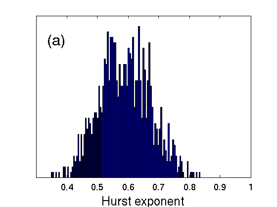
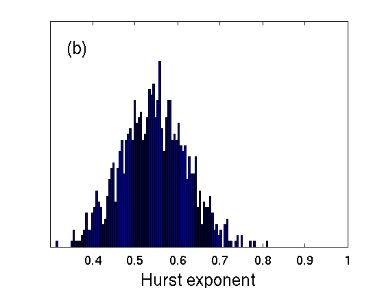
The fact that the method leads to an overestimation of the Hurst exponent for the considered seismic time series means that a fake degree of long-range correlation is originated by an insufficient number of data. This inaccuracy of the Hurst exponent calculated using the method for less than 5000 data points was proved for capital markets [29]. We find that if the four seismic time series are analysed using the method, then the Hurst exponents () obtained with this modified method are smaller than the ones calculated by the method (). We show in the Table 1 the differences between the Hurst exponents calculated using both methods, for the time series of interevent intervals, separation distances, depth differences and magnitude differences.
For this calculations parameters of were chosen by visual inspection of the plots so that they show a linear dependence in each of the cases, while parameters of were chosen equal to 5 in all calculations. By doing this, we assure that the data satisfy the power law in the chosen range of .
| Time series | |||||
|---|---|---|---|---|---|
| Interevent intervals | 0.7642 | 0.7258 | 0.7746 | 0.7907 | 0.7726 |
| Separation distances | 0.7651 | 0.7153 | 0.7871 | 0.7913 | 0.7836 |
| Depth differences | 0.7254 | 0.6883 | 0.7772 | 0.7921 | 0.7826 |
| Magnitude differences | 0.5806 | 0.5521 | 0.5396 | 0.5548 | 0.5556 |
Table 1. Hurst exponent values calculated via the , and methods for the time series of intervent intervals, separation distances, depth differences and magnitude differences.
For the case of time series composed of 1115 data points, as is the case of the four seismic time series analysed in this work (after filtering out events that do not satisfy the Gutenberg-Richter law), a high level of long-range correlation on the data showed up through an overestimation of the Hurst exponents via the method. In other words, the scarcity of data points in the analysis misleads to a fictitious higher long-range correlation. The level of long-range correlation is still not the biggest concern as it is the accurateness of the method to establish if there is correlation or if randomness or anti-correlation govern the dynamics.
Although we have found an overestimation of the correlation level in the seismic time series using the method, i.e. , still Hurst exponents above 0.5 are obtained by using the method except for the time series of magnitude differences. This is an important result of non-randomness for the main parameters of a seismic event, i.e. time, and location of seismic events, meaning they are not arbitrary and therefore a fractal structure describes their behaviour. In this sense, non-randomness implies the presence of patterns behind the structure of the series and potentially a model of future events in terms of time and location could be possibly proposed. Nevertheless, the inclusion of a such model is outside of the goals of this paper. Furthermore, the level of long-range correlation is proportional to the Hurst exponent and the trust values of are obtained via the method. Values of the shown in Table 1 indicate that the persistences associated to the time series of separation distances and interevent intervals are larger than the ones associated to the time series of depth differences and magnitude differences.
We employ the DFA that makes it possible to see whenever the data are affected by different orders of polynomial trends and with this implementation detrended Hurst exponent estimations are feasible (see [45] and references therein). We implement the until the third order to study the existence of trends in seismic time series. This method allows removing trends of order in the data and the comparison between different orders gives an evidence of a specific polynomial order of trends. For the case in which the Hurst exponent calculated with is smaller than the corresponding one with , higher long-range correlations are in fact masked by the presence of trends of order .
Following the analysis via the until the third order, we obtain that the analyzed time series do not present trends. We can make this conclusion starting from the Hurst exponents that we present in Table 1. The differences between , , are so small and they are due to the precision of the algorithm and the differences are between the interval of uncertainty of the method .
5 Colombian subduction zone
The highest level of seismic activity in Colombia is due to the presence of subduction zones. The Nazca plate under the South American plate creates the most representative origin of seismic events in this area. Therefore, with the aim to give more insights about the nature of the seismic fluctuations, the area that encloses the subduction of the Nazca plate beneath the South American plate has been selected for the study that we present in this section, in order to account events with a common physical nature.
We first inspect the behaviour of the Hurst exponent when the maximum window size is varied in the calculation, with the purpose to find the most suitable value of that depends on the number of events considered in time.
In the second part of this section, we explore the agreement in the time evolution between the magnitude and the Hurst exponent on the seismic time series. For this analysis three different maximum window sizes are chosen. Meaningful results for waiting times were reported previously for the Southern México [37]. We extend here these results for the case of time series of interevent intervals associated to the Colombian subduction zone.
5.1 Hurst exponent and maximum window size
The dependence of the Hurst exponent with the maximum window size has been widely studied for time series. However, it has been always difficult to establish criteria that determine the relationship between this parameter and the total number of data points. This dependence is extremely important for the study of the time evolution of the Hurst exponent. Varying the maximum window size and taking a minimum window size of 5 events as a threshold for sufficient statistics, we obtain the behaviour of the Hurst exponent for the time series of interevent intervals in the Colombian subduction zone through the (figure 4).
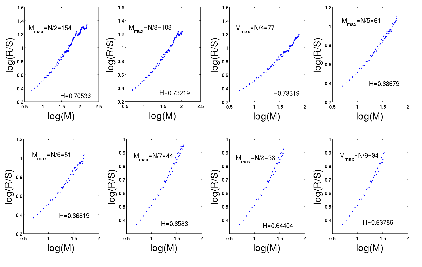
In general one can choose the range of so that the plot follows the linearity or that follows a power law as established in equation 12. In this sense results from figure 4 suggest that the should be around 61, when considering the series with the total number of data .
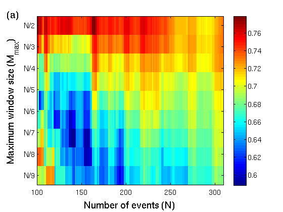
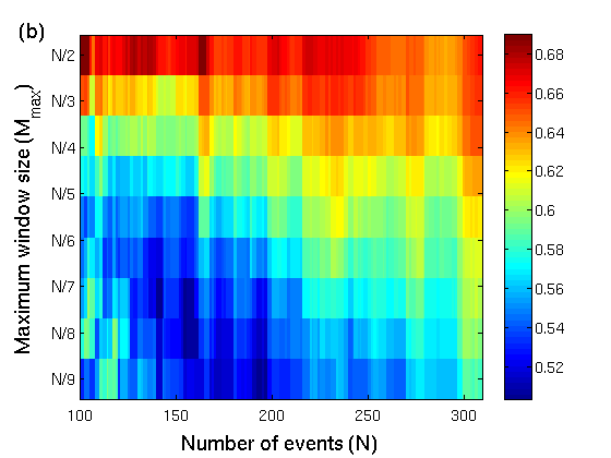
As we wish to study the behaviour of the Hurst exponent as a function of the number of events in the time , it will be necessary to determine a suitable for each . For that purpose we have varied the series from 100 to 340 events and calculated the Hurst exponent for different . It is important to clarify that as depends on the total number of data points considered. We have calculated the Hurst exponent for general employing the and methods, as it is illustrated in Figure 5.
When comparing results from the method (Figure 5(a)) and the method (Figure 5(b)), it is possible to observe that there is an overall constant overestimation of the Hurst exponent calculated via the method of about 0.1. The scarcity of the seismic data points for the subduction zone in the studied years makes the use of the method an ideal one to calculate Hurst exponents.
5.2 Relation between Hurst exponent and magnitude
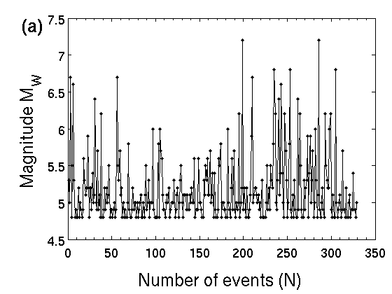
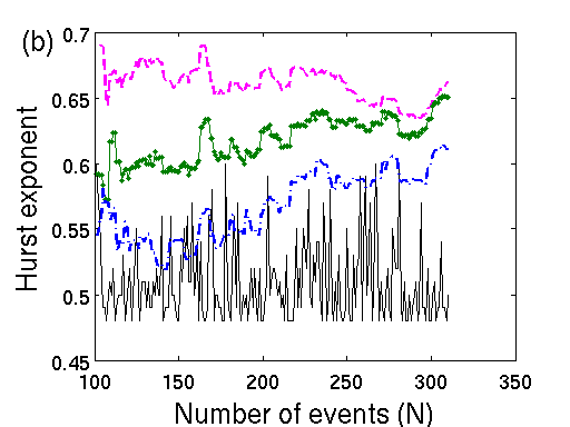
We analyse only those events which follow the Gutenberg-Richter law, with magnitudes between 4.8 and 6 . We can observe in Figure 6(a) different areas of low magnitude that we call low-magnitude gaps. In a previous work [37], it was demonstrated that those low-magnitude gaps are closely related to low correlation levels with values of around 0.5. In the present work, we investigate this relation for the case of the time series of interevent intervals. The results obtained show that is closer to 0.5 for the low-magnitude gap between the 100 and the 175 event (see Figure 6(b)). For the case of the seismic events with magnitudes from 5.5 to 6 , the Hurst exponent becomes also closer to 0.5. This fact means a random behaviour for low magnitude events.
In this work, the relationship obtained between the magnitude and the Hurst exponent can be considered as an extension of the one obtained in [37], but including several values of the maximum window size . The results that we have obtained are shown in Figure 6(b), for three different maximum window size. The upper curve corresponds to , where a correspondence between the magnitude and the Hurst coefficient can not be established. The middle and the lowest curves account values of and respectively, and these curves show certain correlation in the behaviour of the persistence evolution and the magnitude evolution. For both curves, there is a gap from 114 to 174 of low Hurst exponents closer to 0.5. Therefore, a relation between random behaviour and low seismic activity is found for the Colombian subduction zone.
If we regard, for values smaller than , the dependence of respect to the , then the behaviour of the Hurst exponent is reproducing more accurately the evolution on time of the magnitude. This fact could be taken as a desirable threshold for the maximum number of windows on the analysis, since as well as reproduce more accurately the magnitude dynamics than .
6 Conclusions
The seismic time series of interevent intervals, separation distances and depth differences are found to be persistent via the method. Nevertheless, using the method, it is determined that an overestimation of the Hurst exponent affects all the series due to the scarcity of data points (around 2000). Despite the overestimation mentioned above, all the time series under consideration except for the time series of magnitude differences present persistence with , when corrections via the method are taken into account.
Trends were not detected via the comparison between different hierarchies of the until third order for the four time series studied. The differences between , , are attributed to the precision of the algorithm.
For the time series of interevent intervals, the analysis of the Hurst exponent as a function of the time and the minimum number of windows has shown that is ideal for calculations, since it is describing better the dynamics of seismic events. Furthermore, we have found an agreement in the time evolution between low magnitude events and the value of Hurst exponent closer to 0.5 for the gap between 114 and 174 events.
References
- [1] H. E. Stanley, Introduction to phase transitions and critical phenomena, Oxford University Press, London, 1971.
- [2] R. N. Mantegna, and H. E. Stanley, An introduction to econophysics: Correlations and complexity in finance, Cambridge University Press, Cambridge, 2000.
- [3] P. Grau-Carles, Empirical evidence of long-range correlations in stock returns, Physica A 287 (2000) 396-404 .
- [4] P. A. Varotsos, N. V. Sarlis, and E. S. Skordas, Long-range correlations in the electric signals that precede rupture, Phys. Rev. E 66 (2002) 011902.
- [5] S. R. Forrest, and T. A. Witten Jr., Long-range correlations in smoke-particle aggregates, J. Phys. A: Math. Gen. 12 (1979) L109-L117.
- [6] C. -K. Peng, S. V. Buldyrev, A. L. Goldberger, S. Havlin, F. Sciortino, M. Simons, and H. E. Stanley, Long-range correlations in nucleotide sequences, Nature 356 (1992) 168-170.
- [7] T. Hirabayashi, K. Ito, and T. Yoshii, Multifractal analysis of earthquakes, Pure Appl. Geophys. 138 (1992) 591-610.
- [8] C. -K. Peng, S. V. Buldyrev, S. Havlin, M. Simons, H. E. Stanley, and A. L. Goldberger, Mosaic organization of DNA nucleotides, Phys. Rev. E 49 (1994) 1685.
- [9] W. Ebeling, and T. Poschel, Entropy and long range correlations in literary English, Europhys. Lett. 26 (1994) 241-246.
- [10] J. F. Hausdorff, C. -K. Peng, Z. Ladin, J. Y. Wei, and A. L. Goldberger, Is walking a random walk? Evidence for long-range correlations in stride interval of human gait, J. of Appl. Physiol. 78 (1995) 349-358.
- [11] C. -K. Peng, S. Havlin, H. E. Stanley, and A. L. Goldberger, Quantification of scaling exponents and crossover phenomena in nonstationary heartbeat time series, Chaos 5 (1995) 82-87.
- [12] Y. Liu, P. Cizeau, M. Meyer, C. -K. Peng, and H. E. Stanley, Correlations in economic time series, Physica A 245 (1997) 437-440 .
- [13] P. N. Segre, E. Herbolzheimer, and P. M. Chaikin, Long-range correlations in sedimentation, Phys. Rev. Lett 79 (1997) 2574 .
- [14] E. Koscielny-Bunde, A. Bunde, S. Havlin, H. Eduardo Roman, Y. Goldreich, and H. J. Schellnhuber, Indication of a universal persistence law governing athmospheric variability, Phys. Rev. Lett. 81 (1998) 729-732.
- [15] S. Blesic, S. Milosevic, D. Stratimirovic, and M. Ljubisavljevic, Detrended fluctuation analysis of time series of a firing fusimotor neuron, Physica A 268 (1999) 275-282.
- [16] K. Ivanova, and M. Ausloos, Application of the detrended fluctuation analysis (DFA) method for describing cloud breaking, Physica A 274 (1999) 349-354.
- [17] L. Telesca, V. Lapenna, and M. Macchiato, Mono- and multi-fractal investigation of scaling properties in temporal patterns of seismic sequences, Chaos Sol. Frac. 19 (2004) 1-15.
- [18] L. Telesca, and M. Macchiato, Time-scaling properties of the Umbria-Marche 1997-1998 seismic crisis, investigated by the detrended fluctuation analysis of intervent time series, Chaos Sol. Frac. 19 (2004) 377-385.
- [19] S. Gavin, L. McLerran, and G. Moschelli, Longe range correlations and the soft ridge in relativistic nuclear collisions, Phys. Rev. C 79 (2009) 051902(R).
- [20] Y. Ashkenazy, S. Havlin, P. Ch. Ivanov, C.K. Peng, V. Schulte-Frohlinde, and H. E. Stanley, Magnitude and sign scaling in power-law correlated time series, Physica A 323 (2003) 19-41.
- [21] L. Telesca, and M. Lovallo, Investigating non-uniform scaling behaviour in temporal fluctuations of seismicity, Nat. Hazards Earth Syst. Sci. 8 (2008) 973-976.
- [22] G. Michas , F. Vallianatos , and P. Sammonds, Non-extensivity and long-range correlations in the earthquake activity at the West Corinth rift (Greece), Nonlin. Processes Geophys. 20 (2013) 713-724.
- [23] J. Feder, Fractals, Plenum Press, New York, 1988.
- [24] C. Chen, Y. Lee, and Y. Chang, A relationship between Hurst exponents of slip and waiting time data of earthquakes, Physica A 387 (2008) 4643-4648.
- [25] B. B. Mandelbrot, and J. R. Wallis, Noah, Joseph and the operational hydrology, Water Resour. Res. 4 (1968) 909-918.
- [26] H. E. Hurst, Long-term storage capacity of reservoirs, Trans. Am. Soc. Civil Eng. 116 (1951) 770-808.
- [27] B. B. Mandelbrot, and J. R. Wallis, Some long-run properties of geophysical records, Water Resour. Res. 5 (1969) 321-340.
- [28] B. B. Mandelbrot, and J. R. Wallis, Robustness of the rescaled range R/S in the measurement of noncyclic long-run statistical dependence, Water Resour. Res. 5 (1969) 967-988.
- [29] M. A. Sánchez Granero, J. E. Trinidad Segovia, and J. García Pérez, Some comments on Hurst exponent and the long memory processes on capital markets, Physica A 387 (2008) 5543-5551.
- [30] J. E. Trinidad Segovia, M. Fernández-Martínez, and M. A. Sánchez Granero, A note on geometric method-based procedures to calculate the Hurst exponent, Physica A 391 (2012) 2209-2214.
- [31] W. Lo, Long-Term Memory in Stock Market Proces, Econometrica 59 (1991) 98-109.
- [32] J. W. Kantelhardt, E. Koscielny-Bunde, H. H. Rego, S. Havlin, and A. Bunde, Detecting long-range correlations with detrended fluctuation analysis, Physica A 295 (2001) 441-454.
- [33] K. Hu, P. Ch. Ivanov, Z. Chen, P. Carpena, and H. E. Stanley, Effect of trends on detrended fluctuation analysis, Phys. Rev. E 64 (2001) 011114.
- [34] J. F. Eichner, E. Koscielny-Bunde, A. Bunde, S. Havlin, and H. -J. Schellnhuber, Power-law persistence and trends in the atmosphere: A detailed study of long temperature records, Phys. Rev. E 68 (2003) 046133.
- [35] J. W. Kantelhardt, S. A. Zschiegner, E. Koscielny-Bunde, S. Havlin, A. Bunde, and H. E. Stanley, Multifractal detrended fluctuation analysis of nonstationary time series, Physica A 316 (2002) 87-114.
- [36] L. Telesca, M. Lovallo, V. Lapenna, and M. Macchiato, Long-range correlations in two-dimensional spatio-temporal sismic fluctuations, Physica A 377 (2007) 279-284.
- [37] J. Alvarez-Ramirez, J. C. Echeverria, A. Ortiz-Cruz, and E. Hernandez, Temporal and spatial variations of seismicity scaling behavior in Southern Mexico, J. of Geodyn. 54 (2012) 1-12.
- [38] T. Hirata, A correlation between the b value and the fractal dimension of earthquakes, J. of Geophys. Res. 94 (1989) 7507-7514.
- [39] Z. Guo, and Y. Ogata, Correlation between characteristic parameters of aftershock distributions in time, space and magnitude, Geophys. Res. Let. 22 (1995) 993-996.
- [40] Z. Guo, and Y. Ogata, Statistical relations between the parameters of aftershock distributions in time, space and magnitude, J. of Geophys. Res. 102 (1997) 2857-2873.
- [41] P. A. Varotsos, N. V. Sarlis, and E. S. Skordas, Scale-specific order parameter fluctuations of seismicity before mainshocks: Natural time and detendred fluctuation analysis, EPL 99 (2012) 59001.
- [42] U.S. Geological Survey, Earthquake data base, USGS, accessed [Oct. 31, 2011] at URL [http://earthquake.usgs.gov/earthquakes/search/].
- [43] A. Jimenez, Comparison of the Hurst and DEA exponents between the catalogue and its clusters: The California case, Physica A 390 (2011) 2146-2154.
- [44] Y. Xu, and P. W. Burton, Time varying seismicity in Greece: Hurst’s analysis and Monte Carlo simulation applied to a new earthquake catalogue for Greece, Tectonophysics 423 (2006) 125-136.
- [45] K. Domino, The use of the Hurst exponent to predict changes in trends on the Warsaw Stock Exchange, Physica A 390 (2011) 98-109.