LU TP 94-19

October 1994

Estimating nonlinear regression errors without doing regression
Hong Pi
Department of Computer Science & Engineering,
Oregon Graduate Institute, P.O. Box 91000, Portland, Oregon 97291-1000
Carsten Peterson
Department of Theoretical Physics, University of Lund,
Sölvegatan 14A, S-223 62, Lund, Sweden
Email: carsten@thep.lu.se

Abstract:

A method for estimating nonlinear regression errors and their distributions without performing regression is presented. Assuming continuity of the modeling function the variance is given in terms of conditional probabilities extracted from the data. For $N$ data points the computational demand is $N^{2}$. Comparing the predicted residual errors with those derived from a linear model assumption provides a signal for nonlinearity. The method is successfully illustrated with data generated by the Ikeda and Lorenz maps augmented with noise. As a by-product the embedding dimensions of these maps are also extracted.

Background

Most measurements of physical processes are noisy. This is often due to the fact that all independent variables have not been measured. Being able to estimate the noise distribution and its variance directly from data with no assumptions about the underlying signal function is most desirable. It would provide a natural step prior to any modeling of a system (e.g. artificial neural network) since one then knows the optimal performance limit of the fit in advance. Furthermore, methods for filtering data often require prior estimate of noise variance.

To be more concrete, given a table of data $\{(y^{(i)},{\bf x}^{(i)})$, $i=1,2,...,N\}$, where $y$ is the dependent variable and the $d$-dimensional vector ${\bf x}$ denotes the set of explanatory variables, one aims at estimating the variance of $r$ ($\sigma_{r}^{2}$) for

$$\hat{y}=F({\bf x})+r$$ (1)

where $F$ represents the optimum model.

Conventional procedures for estimating $\sigma_{r}^{2}$ are model-based. One fits the data to a model, a particular choice of $F$, and then interprets the deviation of the fit as noise. In the special case of linear regression models [1] where $F$ takes the form

$$\hat{y}=a_{0}+\sum^{d}_{k=1}a_{k}x_{k},$$ (2)

a sample estimate for $\sigma_{r}^{2}$ is explicitly given by

$$\sigma_{r}^{2}=\sigma^{2}-\sum^{d}_{k=1}a_{k}\langle y,x_{k}\rangle$$ (3)

where $\sigma$ denotes the $y$-variable variance and the angled brackets covariances. In this letter we devise a method for estimating the optimum $\sigma_{r}$ when the modeling function $F$ is not restricted to be linear. The estimate does not rely on any conjecture about the form of $F$. The only assumption is that $F$ is uniformly continuous. Loosely speaking we extract probability densities from the data and by sampling data with decreasing bin sizes such that any noise point will appear as a discontinuity. The concept of using the requirement of continuity for establishing dependencies on $x_{k}$ was previously explored in the $\delta$-test method [2], where noise levels had to be estimated by making assumptions about the probability distributions of $r$.

The approach in this work is novel and unique as compared to other methods and also with respect to ref. [2] since no assumption about the distribution of $r$ is needed – $\sigma_{r}^{2}$ is computed directly as an integral over data densities. Actually, the method also disentangles different noise distributions.

Comparing the obtained $\sigma_{r}^{2}$ with what is extracted assuming a linear model in Eq. (3) provides means for establishing nonlinearities.

We illustrate the power of the method with two examples of chaotic time series augmented with noise: the Ikeda [3] and Lorenz [4] maps. In addition to finding noise levels, the method can also be used for determining embedding dimensions.

Method

The goal is to derive a statistical estimate on the variance of $r$ for the optimum model describing Eq. (1). By optimum we mean a model $F$ (Eq. (1)) such that $r$ and $\hat{y}$ are uncorrelated and that $r$ represents identically and independently distributed (i.i.d) noise. Most adaptive algorithms such as neural network models are designed to find such an optimum function.

We use the conditional probabilities defined in the $\delta$-test [2] – for a pair of positive real numbers $\epsilon$ and $\delta$, one constructs directly from the data the conditional probability

$$P(\epsilon|\;\delta)\equiv P(|\Delta y|\leq\epsilon\;|\;|\Delta{\bf x}|\leq\delta)$$ (4)

where $|\Delta{\bf x}|\equiv\max_{k}|x_{k}-x^{\prime}_{k}|$. In the limit $\delta\rightarrow 0$, one obtains

$$P(\epsilon) \equiv \lim_{\delta\rightarrow 0}P(\epsilon|\;\delta)$$ (5)

$$= P(|F({\bf x})-F({\bf x}^{\prime})+r-r^{\prime}|\leq\epsilon\;|\;|{\bf x}-{\bf x}^{\prime}|\rightarrow 0)$$

$$= {\rm Prob}(|\Delta r|\leq\epsilon),$$

where the property of function continuity, $F({\bf x})-F({\bf x}^{\prime})\rightarrow 0$ for ${\bf x}\rightarrow{\bf x}^{\prime}$, is exploited. Eq. (5) establishes a connection between the probability distribution of the residuals $\rho(|\Delta r|)$ to the quantity $P(\epsilon)$, which is directly calculable from the data sample.

The probability density of the residual separation $|\Delta r|$ is given by

$$\rho(|\Delta r|) = -\frac{d}{d|\Delta r|}{\rm Prob}(|\Delta r^{\prime}|>|\Delta r|)$$ (6)

$$= \left[\frac{d}{d\epsilon}P(\epsilon)\right]_{\epsilon=|\Delta r|}.$$

Thus moments of $|\Delta r|$ can be related to $P(\epsilon)$ using eqs. (5, 6). With partial integration one obtains

$$\langle|\Delta r|^{n}\rangle=n\int_{0}^{\infty}d\epsilon\;\epsilon^{n-1}\,[1-P(\epsilon)]$$ (7)

If $r$ is i.i.d one has $\langle(\Delta r)^{2}\rangle=2\sigma_{r}^{2}$. Our estimate for the residual variance of the optimum model is then given by

$$\sigma_{r}^{2}=\int_{0}^{\infty}d\epsilon\;\epsilon\,[1-P(\epsilon)].$$ (8)

We note that the integrand in Eq. (8) suppresses the small $\epsilon$ region. This feature is desirable in limited statistics situations with few high resolution (small $\epsilon$) data points. For higher moments this effect is even further pronounced. In addition to the variance, Eq. (7) of course also provides us with the skewness of the distribution (n=3).

Eq. (6) shows that $P(\epsilon)$ measures the cumulative distribution of the noise separations. It is then possible to discern the noise distribution through $P(\epsilon)$.

In some sense Eq. (7) is equivalent to calculating the expectation value [5],

$$\sigma_{r}^{2}=E[(\Delta y)^{2}|\,|\Delta{\bf x}|\leq\delta]_{\delta\rightarrow 0}.$$ (9)

which may be easier to implement numerically, if one only wants to estimate $\sigma_{r}^{2}$.

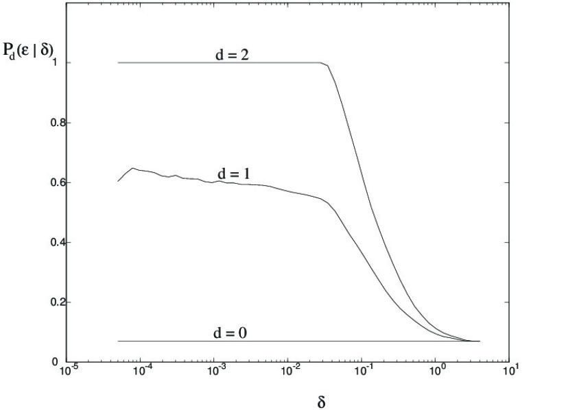
So far we have assumed an infinite amount of data. Some implementation issues are pertinent with limited statistics situations. A suitable binning of the $\log\epsilon$-$\log\delta$ plane for evaluating the probabilities and estimating their statistical errors is given in [2]. In Fig. 1 a typical example of $P(\epsilon|\;\delta)$ is shown. For a fixed $\epsilon$, $P(\epsilon|\;\delta)$ rises and reaches a plateau as $\delta$ decreases. $P(\epsilon)$ is determined by the largest point with acceptable statistics in the plateau region.

$$P(\epsilon)\equiv\max_{\delta>0}P(\epsilon|\,\delta)$$ (10)

The integral of Eq. (8) is easily computed with e.g. the Simpson method.

Figure 1: $P_{d}(\epsilon|\,\vec{\delta})$ as a function of $\delta$ at a fixed $\epsilon=0.108$ for the Hénon map [$x_{t}=1-1.4x^{2}_{t-1}+0.3x_{t-2}$] with N=3000 data points.

Explorations

The Ikeda Map. This system [3] describes the evolution of a laser in a ring cavity with a lossy active medium. In terms of the complex variable $z_{t}=x_{t}+i\,y_{t}$, the map is defined by

$$z_{t+1}=p+B\,z_{t}\exp[i\kappa-\frac{i\alpha}{1+|z_{t}|^{2}}].$$ (11)

Sets of $N=2000$ data points are generated using Eq. (11) with the parameters $p=1.0$, $B=0.9$, $\kappa=0.4$ and $\alpha=6.0$ [10], and with Gaussian noise added to the $x$ component at the each iteration as $x_{t}=x_{t}+r$ with standard deviations $\sigma_{r}$=0.0, 0.01, 0.02 and 0.03 respectively.

Figure 2: The Ikeda map shown in its $x$-$y$ phase space. A Gaussian noise term with standard deviation $\sigma_{r}$ = 0.0 (a), 0.01 (b), 0.02 (c) and 0.03 (d) is added iteratively to the $x_{t}$-component.

We now apply our method to estimate what the error would have been if we had regressed $x_{t}$ on various sets of explanatory variables. The results are shown in

$\sigma_{r}$	0.00		0.01		0.02		0.03
$\sigma_{r}/\sigma$	0.0000		0.0208		0.0424		0.5621
Variables	$\left({\hat{\sigma}_{r}}\right)_{LR}$	$\left({\hat{\sigma}_{r}}\right)_{NL}$	$\left({\hat{\sigma}_{r}}\right)_{LR}$	$\left({\hat{\sigma}_{r}}\right)_{NL}$	$\left({\hat{\sigma}_{r}}\right)_{LR}$	$\left({\hat{\sigma}_{r}}\right)_{NL}$	$\left({\hat{\sigma}_{r}}\right)_{LR}$	$\left({\hat{\sigma}_{r}}\right)_{NL}$
{none}	1.000	1.003	1.000	1.003	1.000	1.003	1.000	1.001
{$x_{t-1}$}	0.997	0.819	0.998	0.792	0.994	0.813	0.642	0.644
{$x_{t-1}$, $y_{t-1}$}	0.887	0.0055	0.889	0.021	0.884	0.044	0.557	0.563

Table 1: Regression errors on $x_{t}$ expressed as fractional errors ${\hat{\sigma}_{r}}$ for various sets of explanatory variables. The subscripts LR and NL stand for linear regression (Eq. (3)) and our method allowing for nonlinear dependencies (Eq. (8)), respectively. Due to the effect of the noise, the noise fraction $\sigma_{r}/\sigma$ varies considerably for differing noise levels.

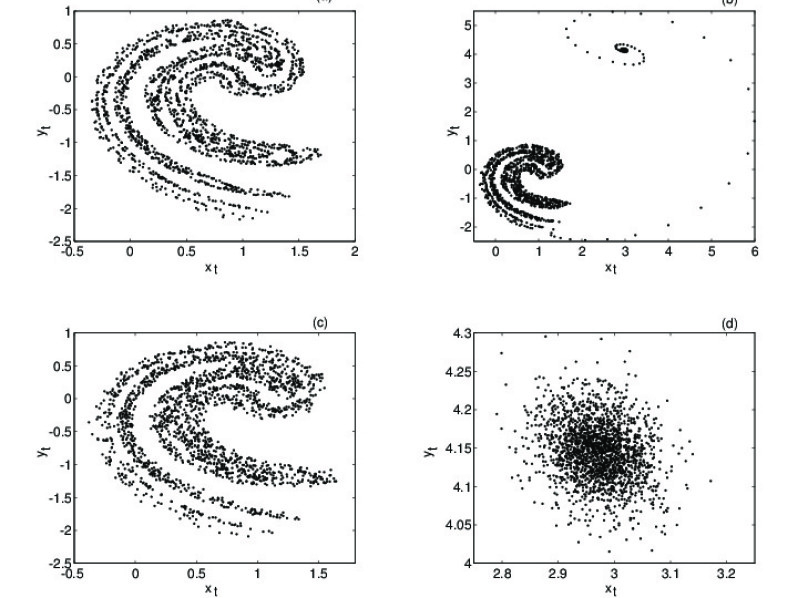
Table 1, which shows that one needs to use the explanatory variable set $\{x_{t-1}$, $y_{t-1}\}$ in order to reduce the residual variance to the optimum level, and our method gives quite accurate estimates on that level in terms of the noise fraction $\sigma_{r}/\sigma$. In the case of $\sigma_{r}=0.0$, the linear regression model gives a noise level 0.887, while our method identifies a negligible noise level ($0.005$). This indicates that the dependency of $x_{t}$ on $x_{t-1}$ and $y_{t-1}$ is predominantly nonlinear. Such a signature of nonlinearity exists as long as the noise level is modest – below $\sigma_{r}=0.02$ in this case. This is consistent with what can be seen in Fig. 2, where the nonlinear structure clearly disappears in (d) when the noise reaches $\sigma_{r}=0.03$.

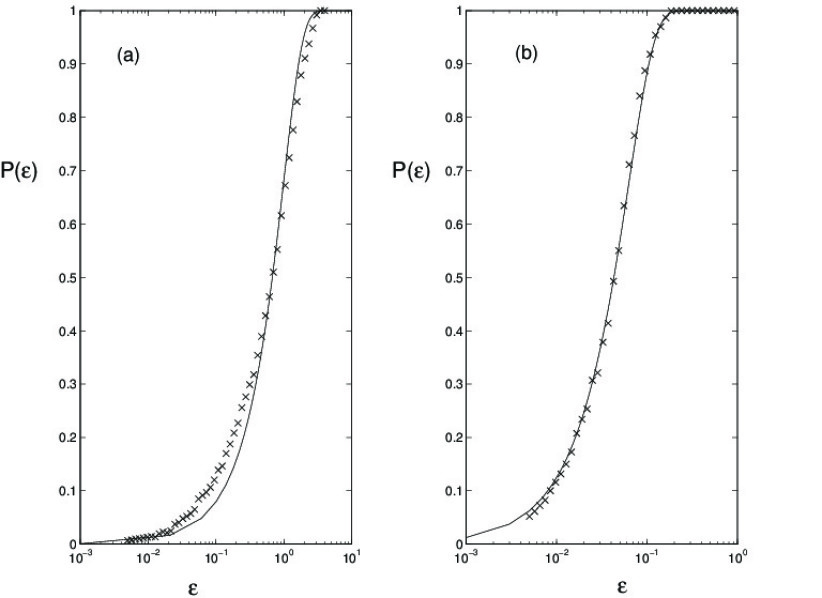
Next we compare $P(\epsilon)$ calculated with our method from data with what is expected from a Gaussian distribution with standard deviation $\sigma_{r}$

$$P(\epsilon)=\int_{0}^{\epsilon}\rho(|\Delta r|)\,d|\Delta r|=erf(\frac{\epsilon}{2\sigma_{r}}),$$ (12)

where $erf$(.) is the error function. In Fig. 3 $P(\epsilon)$ is shown together with the Gaussian analytic expression in Eq. (12). The lines correspond to a least-mean-square fit with $\sigma_{r}$ as parameter. The misfit in Fig. 3a indicates that the residuals based on $x_{t}=F(x_{t-1})+r$ would be non-Gaussian distributed, and that more explanatory variables may be needed to model the process. Fig. 3b shows the $P(\epsilon)$ based on using $x_{t-1}$ and $y_{t-1}$ as the explanatory variables. It indicates that the residuals can be reduced to a Gaussian process if $x_{t}$ is nonlinearly regressed on $x_{t-1}$ and $y_{t-1}$. The best fit results in $\hat{\sigma}_{r}=0.045$ in agreement with the estimate given in Table 1. The absence of sufficient explanatory variables in Fig. 3a emulates additional noise, which also would manifest itself in a skew distribution with a nonvanishing $\langle|\Delta r|^{3}\rangle$.

Figure 3: $P(\epsilon)$ versus $\epsilon$ for the Ikeda map with Gaussian fractional noise $\sigma_{r}/\sigma=0.0424$. The symbols are the values calculated from the data. (a). $P(\epsilon)$ based on using $x_{t-1}$ as the explanatory variable. The line is the analytic expression in Eq. (12) with $\sigma_{r}=0.71$. (b). $P(\epsilon)$ based on using $\{x_{t-1},y_{t-1}\}$ as the explanatory variables. The line is the analytic expression in Eq. (12) with $\sigma_{r}=0.045$.

Let us next turn to the problem of determining the embedding dimension within this scheme assuming that the only data we have at our disposal are the observations of the $x$ component. The variance estimate can then be used to identify the minimum embedding dimension, in a procedure similar to the $\delta$-test [2]. What we need to do is to find the (smallest) set of variables that minimizes the residual error. The results are given in Table 2,

$\sigma_{r}$	0.00		0.02		0.03
$\sigma_{r}/\sigma$	0.0000		0.0424		0.5621
Variables	$\left({\hat{\sigma}_{r}}\right)_{LR}$	$\left({\hat{\sigma}_{r}}\right)_{NL}$	$\left({\hat{\sigma}_{r}}\right)_{LR}$	$\left({\hat{\sigma}_{r}}\right)_{NL}$	$\left({\hat{\sigma}_{r}}\right)_{LR}$	$\left({\hat{\sigma}_{r}}\right)_{NL}$
{none}	1.000	1.003	1.000	1.003	1.000	1.001
{$x_{t-1}$}	0.997	0.819	0.994	0.813	0.642	0.644
{$x_{t-1},\;x_{t-2}$}	0.954	0.505	0.950	0.623	0.622	0.636
{$x_{t-k}\;k=1,..3$}	0.946	0.077	0.946	0.195	0.611	0.635
{$x_{t-k}\;k=1,..4$}	0.936	0.025	0.931	0.074	0.603	0.636
{$x_{t-k}\;k=1,..5$}	0.934	0.026	0.931	0.077	0.598	0.645

Table 2: Regression error on $x_{t}$ for various sets of explanatory variables. Same notation as in Table 1.

from which we see that the residual error ceases to decrease at $k=4$. Therefore we identify the embedding dimension $d_{E}=5$ for the Ikeda map, as long as the noise level is not too high ($\sigma_{r}<$ 0.03). Using the False Nearest Neighbors method, one finds $d_{E}=4$ [10]. As shown in the Table 2, $d_{E}=4$ would result in quite small a residual error of $0.077$ and therefore provides a fairly good embedding. However, $d_{E}=5$ is a better choice.

We observe that in the results presented above, the error estimate $\sigma_{r}$ is very close to $1.0$ when the explanatory variable set is $\{none\}$, as it should be. This provides a consistency check on the applicability of the method on the particular data set. When a significant deviation from $1$ is observed, it indicates that some of the assumptions of the method, e.g. stationarity, is violated in the data set. Also note that the noise estimates $\hat{\sigma}_{r}$ in Table 2 does not match the applied relative noise $\sigma_{r}/\sigma$ exactly, since the regression equation is different from the actual generating process.

The Lorenz Map. A system described by the Lorenz equations [4], which describe meteorological physics,

$$\frac{dx_{t}}{dt} = \sigma[-x_{t}+y_{t}]$$

$$\frac{dy_{t}}{dt} = rx_{t}-y_{t}-x_{t}z_{t}$$ (13)

$$\frac{dz_{t}}{dt} = x_{t}y_{t}-bz_{t}$$

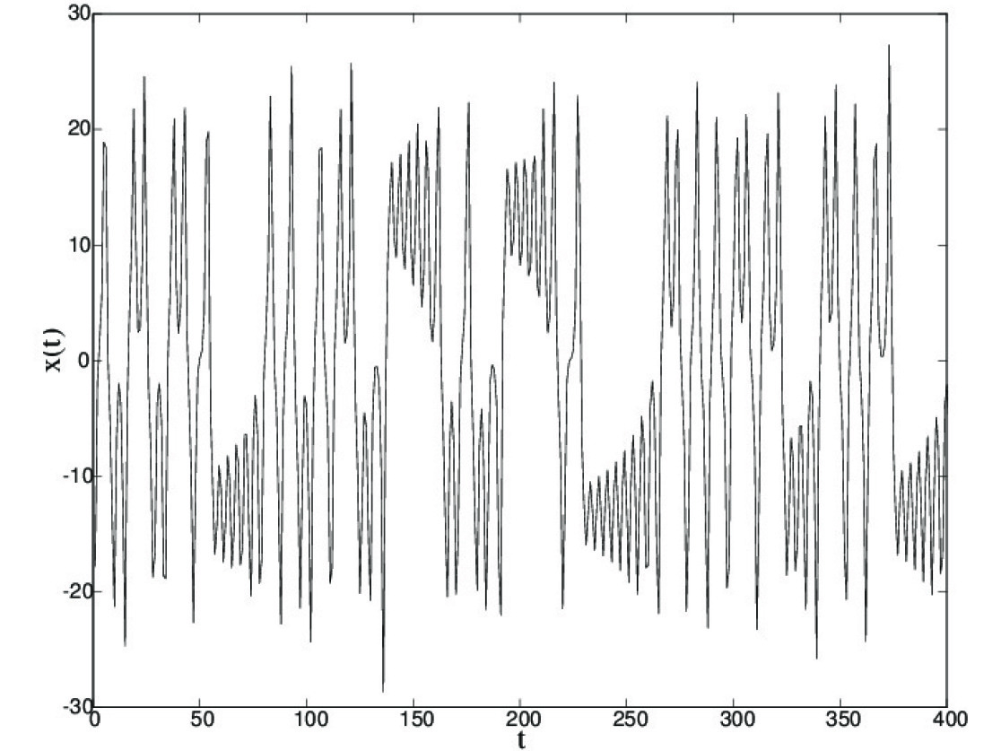
can display low-dimensional chaotic behavior when the parameters are chosen from the chaotic regime [10]. We adopt the parameters $r=45.92$, $b=4.0$ and $\sigma=16.0$ [10], and solve the equations with $\Delta t=0.1$ using the fourth and fifth order Runge-Kutta methods. The method is applied iteratively such that the solutions at $t$ are used as the initial values to the differential equations to obtain the values at $t+0.1$. A portion of the data set is shown in Fig. 4.

Figure 4: The residual variances versus the number of time-lagged variables for the Lorenz-$x_{t}$ data.

Gaussian noise of various variances are superimposed onto the original clean data set. The results of the variance estimates are shown in Table 3. Nonlinearities are evident from the significant differences between the linear regression errors and the nonlinear estimates. Based on the values of $\left({\hat{\sigma}_{r}}\right)_{NL}$ we conclude that three time lag variables are needed to map the variable $x_{t}$. Hence one has $d_{E}=4$ for the Lorenz map.

$\sigma_{r}$	0.00		0.5		1.0
$\sigma_{r}/\sigma$	0.0000		0.0016		0.0062
	$\left({\hat{\sigma}_{r}}\right)_{LR}$	$\left({\hat{\sigma}_{r}}\right)_{NL}$	$\left({\hat{\sigma}_{r}}\right)_{LR}$	$\left({\hat{\sigma}_{r}}\right)_{NL}$	$\left({\hat{\sigma}_{r}}\right)_{LR}$	$\left({\hat{\sigma}_{r}}\right)_{NL}$
$k=0$	1.000	1.000	1.000	1.000	1.000	1.000
$k=1$	0.670	0.520	0.691	0.517	0.693	0.544
$k=2$	0.653	0.084	0.653	0.110	0.657	0.197
$k=3$	0.640	0.01	0.642	0.084	0.646	0.152
$k=4$	0.640	0.008	0.641	0.084	0.646	0.158
$k=5$	0.634	0.008	0.635	0.084	0.640	0.141

Table 3: Regression errors on $x_{t}$ expressed as fractional errors ${\hat{\sigma}_{r}}$ for various numbers of time lag variables for the Lorenz map. $\sigma_{LR}$ gives the linear regression residual error. $\sigma_{NL}$ is the nonlinear estimate from Eq. (9).

The Gaussian noise we imposed have variances of $0.0$, $0.5$, and $1.0$, corresponding to the fractional variances of $0.0$, $0.0016$, and $0.0062$ respectively, which are significantly lower than the estimated fractional residual variances, while in the Ikeda-Map example we had a good match between the true variances and the estimates. This is not an inconsistency since for the Ikeda Map, we applied the noise iteratively:

$$x_{t+1}=F(x_{t-1},y_{t-1})+r,$$ (14)

while in the current example the noise is superimposed to the signal after the entire sequence of the signal is generated. In this case we are dealing with noisy inputs. The equation becomes

$$x_{t+1} = F[x_{t}-r_{t},x_{t-1}-r_{t-1},..]+r_{t+1}$$ (15)

$$= F^{\prime}[x_{t},x_{t-1},..]+r^{\prime}_{t+1}.$$

What the method yields is the variance of the effective noise $r^{\prime}$, which can be quite different from the variance of the superimposed noise $r$.

Summary

We have developed a general method that efficiently extracts noise variances from raw data with no assumptions about the noise distributions. The method handles nonlinear dependencies provided that the underlying function is uniformly continuous and the noise is additive. The method is not limited to determining variances. Any moment of the distribution including skewness and also cumulative distributions can be extracted.

By comparing the extracted noise variances with those derived from assumed linear dependencies, signals of nonlinearities are obtained.

Estimating the variance is very useful for model selection. As a by-product the embedding dimensions are obtained in a way slightly different from that of ref. [2].

We have illustrated the method with two time series examples. The method of course also works in cases with “horizontal dependencies” – variables measured at equal times.

Existing approaches to determine dependencies aimed beyond the linear regime are either based on entropy measures [11, 12] or on elaborate autocorrelation measures [7, 8, 9]. The Mutual Information approach [12] has the shortcoming that it does not disentangle primary dependencies from induced ones. Furthermore, noise levels are not directly extractable. On the other hand its computational effort scales favorable with the number of data points as $N\log N$ as compared to $N^{2}$ with the proposed method. Our approach has its roots in autocorrelation methods [7, 8, 9], but is conceptionally very distinct from these since it is based on continuity. For that reason, in contrast to refs. [7, 8, 9], it extracts the noise levels and ignores induced dependencies.

Acknowledgements. This work was supported in part by the the Swedish Board for Industrial and Technical Development (NUTEK) and the Göran Gustafsson Foundation for Research in Natural Science and Medicine. One of the authors (Pi) gratefully acknowledges the funding provided by the Advanced Research Projects Agency and the Office of Naval Research under grant ONR N000-14-92-J-4062. Pi would also like to thank Brian D. Ripley for helpful discussions.

References

- [1] See e.g. J. D. Hamilton, Time Series Analysis, Princeton University Press (Princeton 1994).
- [2] H. Pi and C. Peterson, Neural Computation 6, 509 (1994).
- [3] K. Ikeda, Opt. Commun. 30, 257 (1979).
- [4] E.N. Lorenz, J. Atmos. Sci. 20, 130 (1963).
- [5] This was suggested to us by Dr. B. D. Ripley.
- [6] M. Hénon, Commun. Math. Phys. 50, 69 (1976).
- [7] P. Grassberger and I. Procaccia, Physica D 9, 189 (1983).
- [8] W.A. Brock et al., “A Test for Independence Based on the Correlation Dimension”, University of Wisconsin Technical Report (1988).
- [9] R. Savit and M. Green, Physica D 50, 95 (1991).
- [10] H. Abarbanel et al., Rev. Mod. Phys. 65, 1331 (1993).
- [11] A.N. Kolmogorov, Dokl. Akad. Nauk. USSR 98, 527 (1959).
- [12] A. M. Fraser, IEEE Trans. Info. Theory IT-35, 245 (1989).