Abstract

We give an overview of Standard Model Higgs boson studies performed at the CDF and DØ experiments at the Tevatron proton-antiproton collider. Combining the results of many individual analyses, most of which use the full data set available, an excess with a significance of 3.0 standard deviations with respect to the Standard Model hypothesis is observed at a Higgs boson mass of 125 $\mathrm{GeV}/c^{2}$. At that mass, the combined best-fit cross section is consistent with the Standard Model prediction. Constraints are also placed on the Higgs boson couplings with fermions and electroweak vector bosons and are consistent with the Standard Model predictions within the uncertainties.

1 Introduction

The Higgs mechanism, first postulated in 1964 [1, 2, 3], is thought to be responsible for electroweak symmetry breaking in the context of the Standard Model (SM) of particle physics [4, 5, 6]. In addition to providing mass terms in the quantum field theoretic Lagrangian density, the mechanism also yields an additional spin-zero particle. In a formal sense, the mass of this particle, the SM Higgs boson, is an unconstrained parameter of the theory. However, various electroweak observables, such as the masses of the $W$ boson and top quark, can place indirect constraints on its mass. Omitting direct searches for the Higgs boson, its predicted mass is $80^{+30}_{-23}$ $\mathrm{GeV}/c^{2}$, based on a fit to measurements of many electroweak quantities [7].

In July 2012, the ATLAS and CMS experiments at the Large Hadron Collider (LHC) reported independent observations of a particle that was consistent with the SM Higgs boson at a mass of 125 $\mathrm{GeV}/c^{2}$ [8, 9], in decent agreement with the electroweak fit prediction. Shortly thereafter, the CDF and DØ experiments at the Tevatron published a joint result showing evidence for the Higgs boson in the $H\to b\bar{b}$ search channel [10], strongly supporting the LHC discoveries. Now that a Higgs boson has been discovered, the best-fit cross sections and couplings can be compared with the predicted 125-$\mathrm{GeV}/c^{2}$ values, both at the LHC and at the Tevatron, providing input on whether the observed particle is consistent with SM expectations.

This paper gives an overview of Higgs boson studies performed at the Tevatron collider at Fermi National Accelerator Laboratory. After briefly introducing the Tevatron and the detectors in Sec. 2, we discuss the Higgs boson search channels and the corresponding primary backgrounds in Sec. 3. We describe the general analysis method of searching for a Higgs boson in Sec. 4, and the statistics technology required for extracting results in Sec. 5. Lastly, results including the upper limits, best-fit cross sections, and Higgs boson coupling constraints are presented in Sec. 6. Full details can be found in Ref. [11] and the references therein. For this paper, we present results only in the context of an SM interpretation.

2 The Tevatron and the Detectors

The Tevatron was a $p\bar{p}$ hadron collider that operated at Fermi National Accelerator Laboratory from 1982 to 2011. The total collision energy in the $p\bar{p}$ center-of-mass frame ($\sqrt{s}$) for Run II (2001 to 2011) was 1.96 TeV. The collision signatures were collected by two experiments—the Collider Detector at Fermilab (CDF) and the DØ experiment—which were positioned around two of the six possible $p\bar{p}$ interaction regions at the Tevatron. Both experiments were multipurpose detectors that contained various systems designed to measure charged-particle momenta, trajectories, and energy deposits. An important component of both detectors was the silicon sensors, which were necessary for identifying secondary vertices displaced from the primary interaction points, thus allowing an inference of the presence of jets that originated from $b$ quarks, which are long-lived compared to light-flavor quarks.

3 Higgs Boson Search Channels

As shown in the left plot of Fig. 1, the Higgs boson production cross sections for $p\bar{p}$ collisions at $\sqrt{s}=1.96$ TeV are on the order of 0.01 to 1 pb, depending on the production mode and the assumed Higgs boson mass in the range $100\leq m_{H}\leq 200$ $\mathrm{GeV}/c^{2}$. The dominant production mode is that of gluon fusion ($gg\to H$ or $p\bar{p}\to H$), whereas the production modes where the Higgs boson is produced in associated with an electroweak boson $V$ (where $V=W$ or $Z$) are suppressed by roughly an order of magnitude but benefit from triggerable signatures from the leptonic decay of the electroweak boson. Additional production modes include vector-boson fusion, where the radiation of two electroweak bosons off of the incoming $p\bar{p}$ pair fuse to form a Higgs boson ($p\bar{p}\to q\bar{q}H$), and the $t\bar{t}H$ production mode, where the Higgs boson is produced alongside a $t\bar{t}$ pair.

Figure 1: Standard Model predictions for the (left) Higgs boson production cross section (figure from Ref. 12), and (right) the Higgs boson branching ratio (figure from Ref. 13) as a function of the assumed Higgs boson mass.

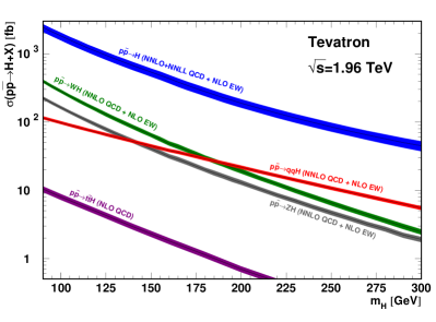
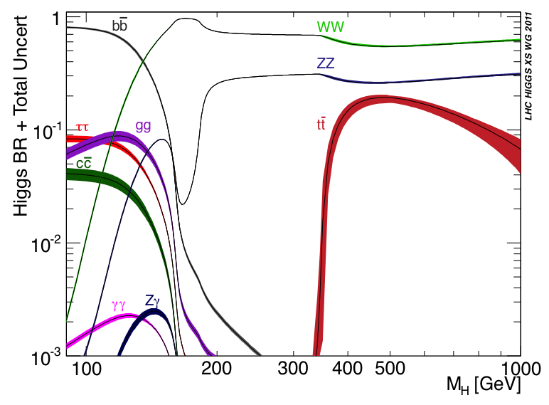
The complete listing of Higgs boson searches published from the Tevatron are listed in Ref. [11], which includes the references for each individual analysis and describes in some detail the overall search strategy. Most of the analyses use the full data set available for the given experiment, which corresponds to roughly $10~{}\mathrm{fb}^{-1}$ of integrated luminosity. This document will only briefly review the general methodology of searching for the Higgs boson at the Tevatron experiments, leaving specific details to Ref. [11] and the references therein. Note that in what follows, the sensitivity of an analysis typically means the sensitivity to exclude the Higgs boson hypothesis.

3.1 High-mass and Low-mass Searches

Higgs boson searches at the Tevatron are classified as high-mass (low-mass) searches if the assumed Higgs boson mass is greater than (less than) 135 $\mathrm{GeV}/c^{2}$, which corresponds to the mass where the $H\to b\bar{b}$ and $H\to W^{+}W^{-}$ branching ratios are approximately equal (see right plot of Fig. 1). For high-mass searches, the $H\to W^{+}W^{-}$ search channel is the most sensitive due to the large $H\to W^{+}W^{-}$ branching ratio. The $H\to W^{+}W^{-}$ final state includes two charged leptons and a significant amount of missing transverse energy due to the neutrinos from the $W\to\ell\bar{\nu}$ decays (where $\ell$ is an electron or muon). For low-mass searches, the dominant decay mode is due to $H\to b\bar{b}$, where the $b\bar{b}$ pair fragments and then hadronizes into a pair of jets, which (as described in Sec. 4.1) can be identified as originating from $b$ quarks. To reduce background contributions from the strong interaction—hereafter, QCD multijet background—the $H\to b\bar{b}$ process is searched for in association with a leptonic decay of an electroweak vector boson. Low-mass searches are therefore typically separated into three categories based on the number of reconstructed charged leptons: $Z\!H\to\ell^{+}\ell^{-}+b\bar{b}$, $W\!H\to\ell\bar{\nu}+b\bar{b}$ and $Z\!H\to\nu\bar{\nu}+b\bar{b}$ analyses, where events with misreconstructed charged leptons are included in the acceptance of the latter two analyses.

Additional low-mass analyses are performed at the Tevatron, such as searches for the $H\to\tau^{+}\tau^{-}$ and $H\to\gamma\gamma$ processes. But as the sensitivities of these searches are significantly less than those described above, we refer the interested reader to Ref. [11] for more details.

In general, hadronic $\tau$ decays are typically not reconstructed due to significant uncertainties in the reconstructible energy. Rather, for Higgs boson searches with charged leptons in the final state, $\tau$ lepton decays are partially included from $\tau\to\ell\bar{\nu}$ processes, where the electron and muon four momenta are well determined.

3.2 Primary Backgrounds

The types of backgrounds encountered in a Higgs boson analysis are highly dependent on the search channel. Whereas the identification of electrons and muons is fairly robust due to the distinct signatures in the calorimeter and muon detectors, respectively, the association of missing transverse energy as originating from neutrinos is not necessarily well established. Significant variations in the jet-energy scale (or jet-energy resolution) for QCD multijet events can create energy imbalances that result in final state signatures that mimic the signal process. To suppress these backgrounds, a typically large value of the missing transverse energy is required (50 to 60 GeV).

Other backgrounds encountered include electrons and photons that mimic jet signatures, and various irreducible backgrounds, such as Drell-Yan processes ($p\bar{p}\to\ell^{+}\ell^{-}+X$), and the SM diboson contributions $WW$, $WZ$ and $ZZ$, whose final states are largely indistinguishable from those of the associated Higgs boson production modes. Many analyses have custom event selection requirements aimed at suppressing these backgrounds to the extent possible.

4 Analysis Methods

The analysis procedures for each Higgs boson search are similar: after imposing a set of event selection criteria on the triggered data, the remaining events are generally separated into those that fall within a signal region, where the measurement is performed, and those that populate various control regions, which are used to validate the background model and analysis methods. In the last few years of Higgs boson analyses at the Tevatron, both experiments have increased signal acceptance by relaxing the lepton-identification and kinematic criteria. The sensitivity to excluding the Higgs boson is further improved by optimizing $b$-jet identification (for low-mass analyses) and by finding ways to separate the signal and background processes in the final histogram used for extracting results, as discussed below.

4.1 $b$-jet identification

The ability to identify a jet as originating from the fragmentation of a $b$ quark is central to searching for the Higgs boson in the $H\to b\bar{b}$ channel. This is achieved by taking advantage of the longer lifetime of the $b$ quark compared to that of a light-flavor quark. With an average lifetime on the order of 1.5 ps, the $b$ quark can travel on the order of a few mm in the transverse plane with respect to the primary interaction vertex before it decays. By using the fine granularity of the silicon detector, the decay vertex of the $b$ quark can be inferred with high confidence, thus allowing a potential matching between the $b$ quark and the corresponding jet as detected by the calorimeter. The goal is to maximize the $b$-jet identification (or $b$-tag) efficiency, while minimizing the false-positive (or mistag) rate.

The final $b$-tagging algorithm used by CDF was specifically optimized for Higgs boson searches [14]. It was a neural network that incorporated inputs from several $b$-tagging algorithms that preceded it, leveraging the correlations between them to further increase $b$-tagging efficiency. The DØ approach was similar, but used a boosted decision tree algorithm instead. For both experiments, a $b$-tag efficiency of better than 50% could be obtained for a corresponding mistag rate of 1%.

4.2 Multivariate techniques

To maximize the sensitivity to excluding the Higgs boson hypothesis, a discriminant function is constructed that seeks to separate the Higgs boson signal from the backgrounds that obscure it. Each event is then assigned a discriminant value and then binned into a histogram that is used to extract results. Various methods are used to construct the discriminant function. The Tevatron analyses typically use multivariate machine-learned algorithms such as neural networks or boosted decision trees, which are trained using Monte Carlo simulated events that are classified as signal or background. The algorithm then “learns” how to distinguish between signal and background events based on the variables that serve as inputs to the discriminant function. An optimal algorithm will result in signal and background distributions of the discriminant value that are maximally separated. This can be approximately achieved by using input variables that exhibit significantly different shapes for signal and background processes.

Many of the Tevatron analyses use several discriminants in a cascade manner. To illustrate, one discriminant may be designed to (e.g.) separate the signal from QCD multijet background; a threshold criterion is then required of the discriminant value for the event. For the surviving events, another discriminant is designed to separate the signal from the remaining backgrounds. The histogram corresponding to this final discriminant is then used for obtaining results. Examples of analyses that use this cascade method are the CDF $Z\!H\to\ell^{+}\ell^{-}+b\bar{b}$ [15] and the DØ $Z\!H\to\nu\bar{\nu}+b\bar{b}$ [16] searches.

Note that the discriminant used in obtaining results is not always the binned histogram of a value that only has an abstract meaning (as in the case of machine-learned nonlinear algorithms). Although a nonlinear algorithm can typically take into account nontrivial correlations between kinematic variables, usually improving the analysis sensitivity, a simple physical quantity can sometimes be nearly as effective. For example, the invariant diphoton mass for the $H\to\gamma\gamma$ searches [17, 18] is used to extract results instead of a multivariate algorithm.

Sections 5 and 6 describe how the discriminants are used to obtain results.

5 Statistical Methods

For each individual analysis, a likelihood is constructed

$$L=\prod_{j}\frac{\mu_{j}^{n_{j}}}{n_{j}!}e^{-\mu_{j}}$$ (1)

which is the product of Poisson probabilities for each of the bins in the discriminant used to obtain results. The observed and expected number of events for each bin are represented by $n_{j}$ and $\mu_{j}$, respectively. In the absence of a Higgs boson signal, $\mu_{j}$ is simply equal to the expected background $b_{j}$. When attempting to exclude a Higgs boson signal, $\mu_{j}$ is allowed to include a signal component $\mu_{j}=Rs_{j}+b_{j}$ where the expected SM Higgs boson signal $s_{j}$ is scaled by $R$, which assesses the sensitivity in the data to a Higgs boson signal.

The presence of systematic uncertainties degrades the sensitivity to excluding a Higgs boson and therefore must be taken into account. This is achieved by introducing a set of nuisance parameters $\boldsymbol{\theta}$ that are expected to follow Gaussian distributions centered at the central value of a given systematic correction, with a root-mean-square width equal to the one-standard deviation uncertainty of the systematic effect. A given nuisance parameter $\theta_{k}$ is thus represented by a Gaussian prior-probability density $\pi_{k}(\theta_{k})$. In principle, the nuisance parameters can be correlated, in which case the appropriate prior-probability density is a multivariate density $\pi(\boldsymbol{\theta})$. The likelihood is thus modified to be:

$$L=\prod_{j}\frac{\mu_{j}^{n_{j}}}{n_{j}!}e^{-\mu_{j}}\times\pi(\boldsymbol{\theta})=\prod_{j}\frac{\mu_{j}^{n_{j}}}{n_{j}!}e^{-\mu_{j}}\prod_{k}\pi_{k}(\theta_{k})$$ (2)

where the second equality applies if $\boldsymbol{\theta}$ represents a set of $k$ independent nuisance parameters $\left\{\theta_{k}\right\}$. As the values of $\mu_{j}$ are allowed to be influenced by the nuisance parameters, the Gaussian prior densities $\pi_{k}$ are truncated at zero to ensure non-negative event yields.

When combining various analysis channels an overall likelihood is constructed, built from the individual likelihoods as given by Eq. (1):

$$\mathcal{L}=\prod_{i}\prod_{j}\frac{\mu_{ij}^{n_{ij}}}{n_{ij}!}e^{-\mu_{ij}}\times\pi(\boldsymbol{\Theta})$$ (3)

where an extra index $i$ has been included to account for each of the analyses that contribute to the combination, and $\boldsymbol{\Theta}$ is the corresponding superset of all nuisance parameters. Measurements are extracted from the data by maximizing the likelihood in the case of the modified frequentist technique used by the DØ experiment, or by maximizing the posterior probability density for the Bayesian technique used by CDF. Both methods are described below, and in what follows, the null (test) hypothesis refers to the SM scenario where the expected number of events excludes (includes) Higgs boson contributions.

5.1 $CL_{S}$ method

The $CL_{S}$ method [19, 20] is the chosen likelihood maximization technique by the DØ experiment. It is frequentist in the sense that no prior assumption is made on the signal strength $R$. A log-likelihood ratio $Q$ is formed as the test statistic, where

$$Q(R)=-2\ln\frac{\mathcal{L}\left(\mathbf{n}|R\right)}{\mathcal{L}\left(\mathbf{n}|0\right)}\ .$$ (4)

The denominator corresponds to the likelihood assuming $R$ is null, and the numerator allows for $R$ to be positive. The binned event yields $\mathbf{n}$ are those that are either observed (as in data) or are produced from pseudo-experiments, as described below.

For a given value of $R$, pseudo-experiments are produced by drawing random variates for $\mathbf{n}$ from both the null and test hypotheses, and then forming distributions in the variable $Q$. According to the Neyman-Pearson lemma [21], this test statistic provides maximum discrimination power between the null hypothesis $H_{0}$ and the test hypothesis $H_{1}$. From each of these hypotheses a $p$-value is calculated that assesses the probability that a result as or more extreme than that observed could be produced under the given hypothesis. For the null hypothesis, the $p$-value is termed $p_{0}$, whereas $p_{1}$ is used for the test hypothesis. The frequentist approach is to exclude the test hypothesis if $p_{1}$ is less than 5%. It is conceivable, however, that a downward fluctuation of the data could exclude not only the test hypothesis but also the null hypothesis. To avoid this situation, the $CL_{S}$ value is constructed, where the standard frequentist result $p_{1}$ is multiplied by $(1-p_{0})^{-1}$. This has the benefit of ensuring conservative results, but it also effectively reduces the sensitivity to excluding the test hypothesis. To obtain confidence levels, the value of $R$ is varied until the $CL_{S}$ quantity is less than the value corresponding to the desired exclusion region.

5.2 Bayesian method

In contrast to DØ, the CDF experiment adopts a Bayesian technique, which requires introducing a prior probability density $\pi(R)$ that parameterizes the “degree of belief” the signal strength $R$ is expected to follow. The relevant function is therefore a multivariate posterior probability density:

$$p(L,R)=\mathcal{C}\times L(\boldsymbol{\theta})\times\pi(R)$$ (5)

where $\mathcal{C}$ is a normalization factor, $L$ is defined by Eq. (1), and the assumed prior density $\pi(R)$ is a non-negative uniform distribution. For clarity, the dependence of $L$ on $\boldsymbol{\theta}$ has been explicitly indicated.

In contrast to maximizing the likelihood $L$, the CDF approach is to marginalize (integrate) over each of the nuisance parameters and extract results based on the marginalized posterior probability density function:

$$p(R)=\mathcal{C}\pi(R)\int L(\boldsymbol{\theta})d\boldsymbol{\theta},$$ (6)

where the only variable not integrated over is the signal strength $R$. How this posterior probability density is used is discussed in Sec. 6.

6 Results

As mentioned earlier, the $CL_{S}$ and Bayesian marginalization techniques are favored by DØ and CDF, respectively, in extracting results on Higgs boson production. In practice, the agreement of the results from both methods is better than 5% with respect to each other. An a priori decision was made to quote Bayesian results in Ref. [11], and that decision is retained here.

6.1 Upper limits on Higgs boson production

To determine the sensitivity a given analysis has to the Higgs boson, many pseudo-experiments are produced that estimate the values of the signal strength one would expect to obtain if no Higgs boson were present (the null hypothesis). For each pseudo-experiment, the $p_{0}(R)$ density is integrated from a lower bound of zero to $R_{95}$, which corresponds to the upper value of the signal strength region that contains 95% of the posterior density. As a Bayesian technique is adopted the limit corresponds to a 95% credibility level (C.L.) upper limit. The distribution of $R_{95}$ values is then used to determine the median-expected sensitivity to the Higgs boson, and the 1- and 2-standard deviation uncertainties on its prediction. The value of $R_{95}$ is then determined for data, which corresponds to the observed limit.

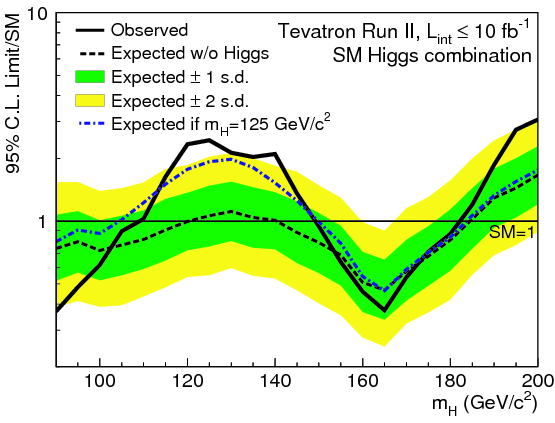
The limit-setting procedure is performed for various Higgs boson masses, depending on the analysis in question. For the Tevatron combination, the union of analyses spans a Higgs boson mass range of $90\leq m_{H}\leq 200$ GeV$/c^{2}$. The Tevatron upper limit combination on Higgs boson production is shown in Fig. 2. The vertical axis represents the value of $R_{95}$, which is in units of the SM prediction. In the mass range $115\leq m_{H}\leq 140$ $\mathrm{GeV}/c^{2}$, the observed data limits are in significant disagreement with the predictions, which assume the null hypothesis. Also plotted is a curve of what one would expect the limit to look like if a SM Higgs boson of mass 125 GeV$/c^{2}$, produced at the SM rate, were present in the data. As can be seen, the SM hypothesis is favored over the null hypothesis in the mass range from roughly 115 to 140 GeV$/c^{2}$. As the primary sensitivity in this mass range results from the $H\to b\bar{b}$ analyses, an excess that is wide is expected if the SM Higgs boson is present, due to significant energy resolution effects of the $b$ jets.

Figure 2: 95% credibility level limits on SM Higgs boson production using Tevatron data (figure from Ref. 11).

6.2 Significance of the excess

The significance of the excess can be determined by estimating the $p$-value of the observed data under the null hypothesis. Before discovery of the Higgs boson by the LHC collaborations, this calculation was performed at each Higgs boson mass under consideration, which also entailed introducing a trials factor that accounted for the look-elsewhere effect. Now that the Higgs boson is known to reside at roughly 125 GeV$/c^{2}$, the Tevatron experiments quote significances just at that mass. For a Higgs boson mass of 125 GeV$/c^{2}$, the Tevatron combination $p$-value corresponds to a significance of 3.0 Gaussian standard deviations, where the expected excess given the SM prediction is 1.9 standard deviations.

6.3 Best-fit cross sections

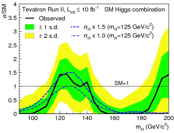
Instead of quoting the 95% C.L. upper limit on the null hypothesis, the posterior distribution $p_{1}(R)$ under the test hypothesis can be used to quote a “best-fit” result, which corresponds to the signal strength that gives the largest posterior probability density. The uncertainty on the best-fit result is given as the shortest $R$ interval that contains 68% of the posterior density. The left plot of Fig. 3 shows the best-fit cross sections, and their 1- and 2-standard deviation uncertainties, across the full Higgs boson mass range considered in Sec. 6.1. The best-fit results are consistent with the SM prediction within uncertainties in the Higgs boson mass range of roughly 115 to 140 GeV$/c^{2}$. Also plotted are the expected best-fit results if the Higgs boson were present at a mass of 125 GeV$/c^{2}$ at the SM production rate, and also at a 50% greater rate, which is more in agreement with what is observed.

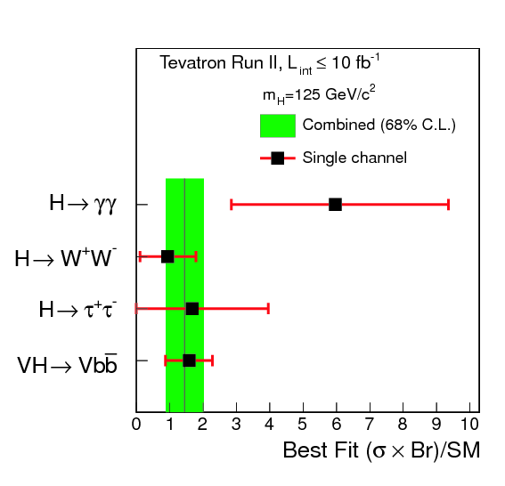
For a Higgs boson mass of 125 GeV$/c^{2}$, the best-fit cross sections and their uncertainties are separately calculated for the $H\to\gamma\gamma$, $H\to W^{+}W^{-}$, $H\to\tau^{+}\tau^{-}$, and $H\to b\bar{b}$ search channels, as shown on the right plot of Fig. 3. All of the best-fit results from the four search channels presented in Fig. 3 are consistent with the SM predictions within uncertainties.

Figure 3: Best-fit cross sections using Tevatron data, assuming the SM Higgs boson hypothesis for (left) all Higgs boson masses considered, and for (right) a mass of 125 GeV$/c^{2}$, separated according to search channel (figures from Ref. 11).

6.4 Constraining Higgs boson couplings

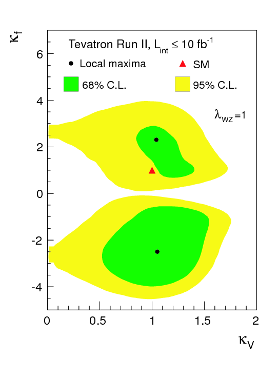
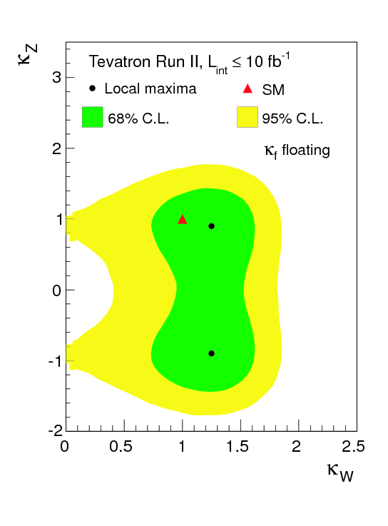
Up until this point, two hypotheses have been considered. Either the null hypothesis is assumed, where one places upper limits on Higgs boson production, or the signal hypothesis is assumed and best-fit cross sections are extracted given the SM prediction. One can also test for the presence of beyond-the-SM physics by assuming the presence of the Higgs boson, but allowing the various Higgs boson couplings to vary. To effect this test, $\kappa_{f}$, $\kappa_{W}$ and $\kappa_{Z}$ scale factors are introduced as coefficients in front of the $H\!f\!f$, $HWW$, and $HZZ$ couplings. For cases when custodial symmetry is assumed, we use $\kappa_{V}\equiv\kappa_{W}=\kappa_{Z}$. The scale factors are normalized in such a way that the SM Higgs boson couplings are recovered when $\kappa_{f}=\kappa_{W}=\kappa_{Z}=1$.

When the $\kappa$ scale factors are introduced, the expressions for Higgs boson production and decay are modified as indicated in Table 1. As the primary sensitivity to the Higgs boson at the Tevatron is in its $H\to b\bar{b}$ searches, the expressions include a cross-term from $\left(\kappa_{f}\kappa_{V}\right)^{2}$, where $\kappa_{V}$ originates from the associated production mode and $\kappa_{f}$ enters from the diquark decay of the Higgs boson. In contrast, some of the searches that are less sensitive to Higgs boson production provide clean avenues to constraining the individual Higgs boson couplings. For example, the $t\bar{t}H$ search does not include any $HVV$ couplings and is thus dependent on only $\kappa_{f}$ in the numerator; and the $V\!H\to V+W^{+}W^{-}$ search does not include any $H\!f\!f$ couplings, thus giving dependence on only $\kappa_{V}$ in the numerator.

Table 1: Modification of production and decay expressions from introducing $\kappa$ scale factors, including an approximate modification for the total Higgs boson decay width, which appears as a denominator.

Process	$\sigma\times\mathcal{B}_{H}$ (w.r.t. SM)
$V\!H\to V+b\bar{b}$	$\propto$	$\left(\kappa_{f}\kappa_{V}\right)^{2}/\left(\frac{3}{4}\kappa_{f}^{2}+\frac{1}{4}\kappa_{V}^{2}\right)$
$t\bar{t}H\to t\bar{t}+b\bar{b}$	$\propto$	$\left(\kappa_{f}^{2}\right)^{2}/\left(\frac{3}{4}\kappa_{f}^{2}+\frac{1}{4}\kappa_{V}^{2}\right)$
$V\!H\to V+W^{+}W^{-}$	$\propto$	$\left(\kappa_{V}^{2}\right)^{2}/\left(\frac{3}{4}\kappa_{f}^{2}+\frac{1}{4}\kappa_{V}^{2}\right)$

The left and right plots of Fig. 4 show the two-dimensional posterior probability density functions of $\kappa_{f}$ vs. $\kappa_{V}$ and $\kappa_{Z}$ vs. $\kappa_{W}$, respectively. As can be seen, the observed results are consistent with the SM predictions at (left) just over one standard deviation, and (right) to well within the one standard-deviation uncertainty.

Figure 4: Two-dimensional posterior probability density functions using Tevatron data testing for the couplings using Tevatron data (figures from Ref. 11).

7 Conclusions

The CDF and DØ Tevatron experiments have performed searches for the SM Higgs boson across an assumed mass range of $90\leq m_{H}\leq 200$ $\mathrm{GeV}/c^{2}$. An excess with a significance of 3.0 standard deviations with respect to the SM hypothesis is observed at a Higgs boson mass of 125 $\mathrm{GeV}/c^{2}$. At that mass, the combined best-fit cross section is consistent with the SM prediction. The Tevatron experiments further constrain the Higgs boson couplings by introducing multiplicative corrections into the cross-section times branching ratio expressions. The data at the Tevatron favor the SM Higgs boson couplings within the uncertainties.

References

- [1] F. Englert and R. Brout, Phys. Rev. Lett. 13, 321 (1964).
- [2] P. W. Higgs, Phys. Rev. Lett. 13, 508 (1964).
- [3] G. S. Guralnik, C. R. Hagen, and T. W. B. Kibble, Phys. Rev. Lett. 13, 585 (1964).
- [4] S. Glashow, Nucl. Phys. 22, 579 (1961).
- [5] S. Weinberg, Phys. Rev. Lett. 19, 1264 (1967).
- [6] A. Salam, Elementary Particle Theory, edited by N. Svartholm (Almqvist and Wiksell, Stockholm, 1968), p. 367.
- [7] H. Flächer et al., Eur. Phys. J. C 60, 543 (2009); Erratum ibid. C 71 1718 (2011).
- [8] G. Aad et al. (ATLAS Collaboration), Phys. Lett. B 716, 1 (2012).
- [9] S. Chatrchyan et al. (CMS Collaboration), Phys. Lett. B 716, 30 (2012).
- [10] T. Aaltonen et al. (CDF and DØ Collaboration), Phys. Rev. Lett. 109, 071804 (2012).
- [11] T. Aaltonen et al. (CDF and DØ Collaborations), Phys. Rev. D 88, 052014 (2013).
- [12] J. Beringer et al. (Particle Data Group), Phys. Rev. D 86, 010001 (2012).
- [13] S. Dittmaier et al. (LHC Higgs Cross Section Working Group), CERN-2013-004, arXiv:1307.1347 (2013).
- [14] J. Freeman et al., Nucl. Instrum. Methods Phys. Res., Sect. A 697, 64 (2013).
- [15] T. Aaltonen et al. (CDF Collaboration), Phys. Rev. Lett. 109, 111803 (2012).
- [16] V. M. Abazov et al. (DØ Collaboration), Phys. Lett. B 716, 285 (2012).
- [17] T. Aaltonen et al. (CDF Collaboration), Phys. Lett. B 717, 173 (2012).
- [18] V. M. Abazov et al. (DØ Collaboration), Phys. Rev. D 88, 052007 (2013).
- [19] T. Junk, Nucl. Instrum. Methods Phys. Res., Sect. A 434, 435 (1999).
- [20] A. L. Read, J. Phys. G 28, 2693 (2002).
- [21] J. Neyman and E. S. Pearson, Phil. Trans. R. Soc. Lond. A 231, 694-706, 289-337 (1933).