\NAT@set@cites

Staffing Call Centers with Uncertain Arrival Rates and Co-sourcing

YaลŸar Levent KoรงaฤŸa

Syms School of Business, Yeshiva University, Belfer Hall 403/A, New York, NY 10033, kocaga@yu.edu


Mor Armony
Stern School of Business, New York University, KMC 8โ€“62, New York, NY, 10012, marmony@stern.nyu.edu


Amy R. Ward
Marshall School of Business, University of Southern California, Bridge Hall 401H Los Angeles, CA, 90089, amyward@marshall.usc.edu

In a call center, staffing decisions must be made before the call arrival rate is known with certainty. Then, once the arrival rate becomes known, the call center may be over-staffed, in which case staff are being paid to be idle, or under-staffed, in which case many callers hang-up in the face of long wait times. Firms that have chosen to keep their call center operations in-house can mitigate this problem by co-sourcing; that is, by sometimes outsourcing calls. Then, the required staffing N๐‘N depends on how the firm chooses which calls to outsource in real-time, after the arrival rate realizes and the call center operates as a M/M/N+M๐‘€๐‘€๐‘๐‘€M/M/N+M queue with an outsourcing option. Our objective is to find a joint policy for staffing and call outsourcing that minimizes the long run average cost of this two-stage stochastic program when there is a linear staffing cost per unit time and linear costs associated with abandonments and outsourcing.

We propose a policy that uses a square-root safety staffing rule, and outsources calls in accordance with a threshold rule that characterizes when the system is โ€œtoo crowdedโ€. Analytically, we establish that our proposed policy is asymptotically optimal, as the mean arrival rate becomes large, when the level of uncertainty in the arrival rate is of the same order as the inherent system fluctuations in the number of waiting customers for a known arrival rate. Through an extensive numerical study, we establish that our policy is extremely robust. In particular, our policy performs remarkably well over a wide range of parameters, and far beyond where it is proved to be asymptotically optimal.

Keywords: Call center operations; outsourcing; co-sourcing; staffing; overflow routing; abandonment; parameter uncertainty.

1 Introduction

Call centers have become ubiquitous in business. Today, every Fortune 500 company has at least one call center, and the average Fortune 500 company employs 4500 call center agents (who may be distributed across more than one site) (Gilson and Khandelwal, 2005). For many companies, the call center is a primary point-of-contact with their customers. Hence a well-run call center promotes good customer relations, and a poorly-managed one hurts them. But call center management is difficult.

A call center manager faces the classical operational challenge of determining appropriate staffing levels throughout the day and week in order to meet a random and time-varying call volume. This is extremely difficult especially when call arrival rate is itself random, as was empirically shown in Brown etย al. (2005) and Maman (2009), among others. When staffing levels are too low, customers are put on hold, and many hang up in frustration while waiting for an agent to take their call. But when staffing levels are too high, the call center manager ends up paying staff to be idle.

One option in managing this uncertainty is for a company to outsource its call center operations. Then, the challenges of call center management can be handled by a vendor firm whose primary focus is call center operations. That vendor can pool demand amongst various companies, thereby lowering variability, which should allow for more accurate demand forecasts, and so better staffing decisions. However, it is also true that many companies are reluctant to relinquish control of their call center operations. This is evidenced by a recent survey from the Incoming Call Management Instituteย (ICMI, 2006): only 7.9% out of 279 call center professionals used an outside vendor to handle most or all of their calls. One reason for that are the โ€œhidden costs of outsourcingโ€ (Kharif, 2003), which include service quality costs that are hard to explicitly quantify. As a result, many of these companies prefer to co-source; that is, to outsource some, but not all, of their calls.

We study a co-sourcing structure in which the vendor charges the company a fee per call outsourced, which is consistent with the pay-per-call (PPC) co-sourcing structure analyzed inย AkลŸin etย al. (2008). Then, the company can decide on a call-by-call basis which calls to answer in-house and which calls to route to the vendor. This is helpful because call centers typically make their daily staffing decisions at least a week in advance, before the actual arrival rate to the call center for a given day is known. If the planned staffing is sufficient to handle the mean arrival rate, then the company needs to outsource only a small fraction of calls in order to handle the inherent variability that results in congestion every so often. On the other hand, if the planned staffing is insufficient to handle the mean arrival rate, then the company can outsource a large fraction of its calls, thereby preventing high congestion levels.

The relevant question for this paper is: how do we decide on staffing levels when the arrival rate is uncertain and the aforementioned co-sourcing option is present? To answer this question, we begin with one simple and widely used queueing model of a call center, the Erlang A or M/M/N+M๐‘€๐‘€๐‘๐‘€M/M/N+M (see, for example, Section 4.2.2 inย Gans etย al. (2003)), and add uncertainty in the arrival rate and an outsourcing option. Then, our model for the call center is a multi-server queue with a doubly stochastic time-homogeneous Poisson arrival process, exponential service times, and exponential times to abandonment. Although this model ignores the time-varying nature of the arrival rate over the course of each day, there is call center literature that discusses how to use the Erlang A model to make staffing decisions for time-varying arrival rates, using the โ€œstationary independent period by period approachโ€ (SIPP); seeย Green etย al. (2001),ย Gans etย al. (2003),ย Aksin etย al. (2007), andย Liu and Whitt (2012) for more discussion. We suppose that a similar approach can be adopted here to accommodate the added feature of arrival rate uncertainty.

The control decisions in our model are (a) an upfront staffing decision and (b) real-time call outsourcing (routing) decisions. Recall that staffing decisions are made on a much longer time horizon and well before the timing of the control decisions. In particular, these decisions are made on two different time scales. This means that we have a two stage stochastic program: The staffing decisions are made in the first stage, before the arrival rate is known, and the outsourcing decisions are made in the second stage, after the arrival rate is known. Then, the outsourcing decisions can depend on the actual arrival rate even though the staffing decisions cannot.

Our objective is to propose a policy for staffing and outsourcing under the assumption of linear staffing cost and linear abandonment and outsourcing costs. Then, for each arriving customer that cannot be immediately served, there is a tension between choosing to outsource that customer (and paying the outsourcing fee) or having that customer wait for an in-house agent (and risking incurring an abandonment cost). In summary, we are solving a joint staffing and routing control problem for a (modified) Erlang A model with an uncertain arrival rate and an outsourcing option.

The three main contributions in this paper are:

  • โ€ข

    The modeling contribution is the formulation of a joint staffing and outsourcing problem for a call center that has access to co-sourcing, and must make staffing decisions when there is arrival rate uncertainty. This modeling framework can be used to study more general joint staffing and control problems in call centers that have been previously studied in the literature under the assumption of a known arrival rate.

  • โ€ข

    The application contribution is the development of a square root safety staffing and threshold outsourcing policy that we numerically show to be extremely robust over the entire parameter space. This robustness may come as no surprise for readers who are familiar with related literature such asย Borst etย al. (2004) andย Gurvich etย al. (2013). However, the existing literature has not addressed the issue of robustness in the context of random arrival rates and dynamic control, nor can this robustness be readily explained using existing results.

  • โ€ข

    The technical contribution is the proof that our proposed square root safety staffing and threshold outsourcing policy is asymptotically optimal, as the mean arrival rate becomes large, when the level of uncertainty in the arrival rate is of the same order as the inherent system stochasticity (which is of the order of the square root of the mean of the arrival rate).

The remainder of this paper is organized as follows. First, we review the most relevant literature. Next, in Section 2, we describe our model in detail. In Section 3, we present the exact (non-asymptotic) analysis which leads to an algorithm to compute the optimal policy numerically. However, that algorithm does not provide insight into the structure of an optimal policy, and so, in Section 4, we perform an asymptotic analysis under the assumption that the level of uncertainty in the arrival rate is of the same order as the inherent system stochasticity. That asymptotic analysis motivates us to propose, in Sectionย 5, a square root safety staffing and threshold outsourcing policy that is universal in the sense that there is no assumption on the level of uncertainty in the arrival rate. We evaluate the performance of our universal policy numerically in Section 6. We make concluding remarks in Section 7. All proofs and additional numerical results can be found in the electronic companion (EC).

Literature Review

Previous work on joint staffing and routing problems in call centers includes Gurvich etย al. (2008) who study staffing and dynamic routing in call centers with multiple customer classes and a single server pool, Armony and Mandelbaum (2011) who consider the symmetric case of a single customer type and a heterogeneous server pool, and Gurvich and Whitt (2010) who consider multiple customer classes and a heterogeneous server pool. These papers study the staffing and dynamic routing problems within the Halfin-Whitt heavy traffic regime, pioneered by Halfin and Whitt (1981), and extended to include abandonments by Garnett etย al. (2002). This is also known as the Quality and Efficiency Driven (QED) heavy traffic regime. The key idea is to approximate the behavior of call centers that are modeled as multi-server queues with that of their limiting diffusions. The limiting diffusion arises from a specific relationship between the arrival rate and the staffing level as both grow large without bound. Our work is different than the aforementioned papers in that our model is pertinent to situations where the arrival rate is not known when staffing decisions are made, and thus has to be inferred or forecasted using available historical data.

Given a staffing level and a realized arrival rate, our dynamic outsourcing decision is equivalent to the admission control problem studied in KoรงaฤŸa and Ward (2010). The equivalence follows because we do not explicitly model the vendor firm and assume it has ample capacity to handle the outsourced calls. KoรงaฤŸa and Ward (2010) show that a threshold admission control policy is optimal, and characterize a simple form for the threshold level that is asymptotically optimal when the staffing level is assumed to be such that the system operates in the QED regime. In contrast, this paper explicitly models the staffing decisions and has a random arrival rate.

There is a growing body of literature that studies staffing for call centers with uncertain arrival rates including (in chronological order) Chen and Henderson (2001), Jongbloed and Koole (2001), Ross (2001), Bassamboo etย al. (2005), Bassamboo etย al. (2005), Whitt (2006), Bassamboo etย al. (2006), Steckley etย al. (2009), Maman (2009), Bassamboo and Zeevi (2009), Gurvich etย al. (2010), Robbins and Harrison (2010), Bassamboo etย al. (2010), Mehrotra etย al. (2010), Gans etย al. (2012), and Zan etย al. (2013). The two works most closely related to ours are Maman (2009) and Bassamboo etย al. (2010), and we discuss each in turn.

The focus of Maman (2009) is to extend the QED staffing formula under a general form of arrival uncertainty. Our asymptotic optimality result assumes a special case of the form of the arrival rate uncertainty presented in that paper. However, that paper does not explicitly study the cost minimizing staffing and does not model routing decisions, as we do.

Bassamboo etย al. (2010) propose a staffing policy for an M/M/N+M๐‘€๐‘€๐‘๐‘€M/M/N+M queue in which the arrival rate is random, and there is no outsourcing option. They establish that a simple newsvendor based staffing policy performs extremely well when the order of uncertainty in the arrival rate exceeds the order of the inherent system stochasticity. In contrast, we establish the asymptotic optimality of our proposed policy when the aforementioned two magnitudes are the same. Then, in our numeric study, we adapt their policy to our setting with outsourcing, in order to evaluate policy robustness.

In relation to the literature on call center outsourcing (see, for example, Zhou and Ren (2011)), our paper is most similar to AkลŸin etย al. (2008). In contrast to most papers in this literature, which assumes all calls will be outsourced, AkลŸin etย al. (2008) considers the contract design problem of a company which faces an uncertain call volume, and can outsource part of its calls by choosing between a capacity-based and volume-based contract that is pay-per-call. Although both AkลŸin etย al. (2008) and our model study co-sourcing decisions which are driven by call volume uncertainty, AkลŸin etย al. (2008) focuses on the optimal contract choice, whereas we focus on the in-house staffing and dynamic routing decisions and assume the contract.

2 Model Description

We model the in-house call center (which we henceforth refer to as โ€œthe call centerโ€ or โ€œthe systemโ€) as an M/M/N+M๐‘€๐‘€๐‘๐‘€M/M/N+M queueing system in which the arrival rate is uncertain. We let ฮ›ฮ›\Lambda denote the random arrival rate with cdf Fฮ›subscript๐นฮ›F_{\Lambda}, and we let l๐‘™l denote a particular realization of ฮ›ฮ›\Lambda. We assume that ฮ›ฮ›\Lambda is a non-negative random variable with mean Eโ€‹[ฮ›]=ฮป๐ธdelimited-[]ฮ›๐œ†E\left[\Lambda\right]=\lambda. For ease of exposition, we assume the mean service time is 1, so that we can think of measuring time in terms of the mean time to serve an arrival. The mean patience time is 1/ฮณ1๐›พ1/\gamma.

The call center manager must make two decisions: the upfront staffing level N๐‘N, and the dynamic outsourcing decision. The staffing level N:=Nโ€‹(Fฮ›)assign๐‘๐‘subscript๐นฮ›N:=N(F_{\Lambda}) must be set before the arrival rate ฮ›ฮ›\Lambda is realized, based on the knowledge of its distribution. After the arrival rate ฮ›ฮ›\Lambda is realized as l๐‘™l, every arriving call can be either accepted into the system, or routed to the outsourcing vendor. Then, the routing control policy ฯ€:=ฯ€โ€‹(N,l)assign๐œ‹๐œ‹๐‘๐‘™\pi:=\pi(N,l) is in general a function of the staffing level N๐‘N and l๐‘™l. The notation ฯ€โ€‹(N,ฮ›)๐œ‹๐‘ฮ›\pi(N,\Lambda) refers to a routing policy that may depend on the actual realization l๐‘™l of ฮ›ฮ›\Lambda. Any stationary routing control policy ฯ€=(ฯ€n:nโˆˆ{0,1,โ€ฆ})\pi=(\pi_{n}:n\in\{0,1,\ldots\}) is a vector, where ฯ€nโˆˆ[0,1]subscript๐œ‹๐‘›01\pi_{n}\in[0,1] denotes the probability that a customer is accepted into the system when there are n๐‘›n customers currently present there. We let ฮ ฮ \Pi be the set of all such vectors. An admissible policy

u:=(N,ฯ€(N,ฮ›))=(N,(ฯ€n(N,ฮ›):nโˆˆ{0,1,โ€ฆ}))u:=(N,\pi(N,\Lambda))=(N,(\pi_{n}(N,\Lambda):n\in\{0,1,\ldots\}))

sets the staffing level as a non-negative integer N๐‘N, and, after the arrival rate ฮ›ฮ›\Lambda realizes as l๐‘™l, controls outsourcing decisions dynamically by routing calls according to the policy ฯ€โ€‹(N,l)โˆˆฮ ๐œ‹๐‘๐‘™ฮ \pi(N,l)\in\Pi.

After the arrival rate l๐‘™l realizes, the system operates as a birth and death process with birth rate lโ€‹ฯ€n๐‘™subscript๐œ‹๐‘›l\pi_{n} and death rates

ฮผn=minโก(N,n)+ฮณโ€‹[nโˆ’N]+.subscript๐œ‡๐‘›๐‘๐‘›๐›พsuperscriptdelimited-[]๐‘›๐‘\mu_{n}=\min(N,n)+\gamma[n-N]^{+}.

It is straightforward to solve the balance equations for the steady-state distribution for the number-in-system process, from which it follows that the following performance measures are well-defined:

Pฯ€โ€‹(ab;l)subscript๐‘ƒ๐œ‹ab๐‘™\displaystyle P_{\pi}(\mbox{ab};l) =\displaystyle= the probability an entering customer abandons;
Pฯ€โ€‹(out;l)subscript๐‘ƒ๐œ‹out๐‘™\displaystyle P_{\pi}(\mbox{out};l) =\displaystyle= the probability an arriving customer is routed to the outsourcer.the probability an arriving customer is routed to the outsourcer\displaystyle\mbox{ the probability an arriving customer is routed to the outsourcer}.

The objective of the system manager is to minimize the expected long-run average cost, when there are costs due to customer abandonment, routing customers to the outsourcing vendor, and staffing costs. Every customer that abandons the system before receiving service costs a๐‘Ža and the per call cost of routing to the outside vendor is p๐‘p. Then, the long-run average operating cost associated with ฯ€โˆˆฮ ๐œ‹ฮ \pi\in\Pi when the arrival rate realizes as l๐‘™l and the staffing level is N๐‘N is

zฯ€:=zฯ€โ€‹(N,l)=pโ€‹lโ€‹Pฯ€โ€‹(out;l)+aโ€‹lโ€‹Pฯ€โ€‹(ab;l).assignsubscript๐‘ง๐œ‹subscript๐‘ง๐œ‹๐‘๐‘™๐‘๐‘™subscript๐‘ƒ๐œ‹out๐‘™๐‘Ž๐‘™subscript๐‘ƒ๐œ‹ab๐‘™z_{\pi}:=z_{\pi}(N,l)=plP_{\pi}(\mbox{out};l)+alP_{\pi}(\mbox{ab};l). (2.1)

This is expressed as a random variable by writing each of the performance measures of interest as random variables, as follows

zฯ€โ€‹(N,ฮ›)=pโ€‹ฮ›โ€‹Pฯ€โ€‹(out;ฮ›)+aโ€‹ฮ›โ€‹Pฯ€โ€‹(ab;ฮ›).subscript๐‘ง๐œ‹๐‘ฮ›๐‘ฮ›subscript๐‘ƒ๐œ‹outฮ›๐‘Žฮ›subscript๐‘ƒ๐œ‹abฮ›z_{\pi}(N,\Lambda)=p\Lambda P_{\pi}(\mbox{out};\Lambda)+a\Lambda P_{\pi}(\mbox{ab};\Lambda).

For a given realization l๐‘™l of ฮ›ฮ›\Lambda, zoptโ€‹(N,l)superscript๐‘งopt๐‘๐‘™z^{\mbox{\tiny{opt}}}(N,l) denotes the minimum cost, and ฯ€optโ€‹(N,l)โˆˆฮ superscript๐œ‹opt๐‘๐‘™ฮ \pi^{\mbox{\tiny{opt}}}(N,l)\in\Pi is a policy that achieves that minimum cost. The associated random varaiables are zoptโ€‹(N,ฮ›)superscript๐‘งopt๐‘ฮ›z^{\mbox{\tiny{opt}}}(N,\Lambda) and ฯ€optโ€‹(N,ฮ›)superscript๐œ‹opt๐‘ฮ›\pi^{\mbox{\tiny{opt}}}(N,\Lambda). The expected long-run average cost under the policy u=(N,ฯ€)=(N,ฯ€โ€‹(N,ฮ›))๐‘ข๐‘๐œ‹๐‘๐œ‹๐‘ฮ›u=(N,\pi)=(N,\pi(N,\Lambda)), with respect to the random arrival rate ฮ›ฮ›\Lambda, is

๐’žโ€‹(u)=cโ€‹N+Eโ€‹[zฯ€โ€‹(N,ฮ›)].๐’ž๐‘ข๐‘๐‘๐ธdelimited-[]subscript๐‘ง๐œ‹๐‘ฮ›\mathcal{C}(u)=cN+E\left[z_{\pi}\left(N,\Lambda\right)\right]. (2.2)

We would like to find a staffing level Noptsuperscript๐‘optN^{\mbox{\tiny{opt}}} and a routing control policy ฯ€optโ€‹(N,ฮ›)superscript๐œ‹opt๐‘ฮ›\pi^{\mbox{\tiny{opt}}}(N,\Lambda) that achieves the minimum long-run average cost

๐’žopt:=infu๐’žโ€‹(u)=minNโˆˆ{0,1,2,โ€ฆ}โกcโ€‹N+Eโ€‹[zoptโ€‹(N,ฮ›)].assignsuperscript๐’žoptsubscriptinfimum๐‘ข๐’ž๐‘ขsubscript๐‘012โ€ฆ๐‘๐‘๐ธdelimited-[]superscript๐‘งopt๐‘ฮ›\mathcal{C}^{\mbox{\tiny{opt}}}:=\inf_{u}\mathcal{C}(u)=\min_{N\in\{0,1,2,\ldots\}}cN+E\left[z^{\mbox{\tiny{opt}}}(N,\Lambda)\right]. (2.3)
Remark 1.

(Including waiting costs.) The objective function in (2.2) can be modified to include a customer waiting cost by modifying (2.1) as follows. Suppose the cost for one customer to wait one time unit is wโ‰ฅ0๐‘ค0w\geq 0. Then, (2.1) becomes

zฯ€:=zฯ€โ€‹(N,l)=pโ€‹lโ€‹Pฯ€โ€‹(out;l)+aโ€‹lโ€‹Pฯ€โ€‹(ab;l)+wโ€‹lโ€‹(1โˆ’Pฯ€โ€‹(out;l))โ€‹Wยฏฯ€โ€‹(l),assignsubscript๐‘ง๐œ‹subscript๐‘ง๐œ‹๐‘๐‘™๐‘๐‘™subscript๐‘ƒ๐œ‹out๐‘™๐‘Ž๐‘™subscript๐‘ƒ๐œ‹ab๐‘™๐‘ค๐‘™1subscript๐‘ƒ๐œ‹out๐‘™subscriptยฏ๐‘Š๐œ‹๐‘™z_{\pi}:=z_{\pi}(N,l)=plP_{\pi}(\mbox{out};l)+alP_{\pi}(\mbox{ab};l)+wl(1-P_{\pi}(\mbox{out};l))\overline{W}_{\pi}(l),

where Wยฏฯ€โ€‹(l)subscriptยฏ๐‘Š๐œ‹๐‘™\overline{W}_{\pi}(l) is the steady-state average waiting time, including both abandoning and served customers. Letting Qยฏฯ€โ€‹(l)subscriptยฏ๐‘„๐œ‹๐‘™\overline{Q}_{\pi}(l) denote the steady-state average number of customers waiting in queue to be served, it follows from Littleโ€™s law that

lโ€‹(1โˆ’Pฯ€โ€‹(out;l))โ€‹Wยฏฯ€โ€‹(l)=Qยฏฯ€โ€‹(l),๐‘™1subscript๐‘ƒ๐œ‹out๐‘™subscriptยฏ๐‘Š๐œ‹๐‘™subscriptยฏ๐‘„๐œ‹๐‘™l(1-P_{\pi}(\mbox{out};l))\overline{W}_{\pi}(l)=\overline{Q}_{\pi}(l),

and so

zฯ€=pโ€‹lโ€‹Pฯ€โ€‹(out;l)+aโ€‹lโ€‹Pฯ€โ€‹(ab;l)+wโ€‹Qยฏฯ€โ€‹(l).subscript๐‘ง๐œ‹๐‘๐‘™subscript๐‘ƒ๐œ‹out๐‘™๐‘Ž๐‘™subscript๐‘ƒ๐œ‹ab๐‘™๐‘คsubscriptยฏ๐‘„๐œ‹๐‘™z_{\pi}=plP_{\pi}(\mbox{out};l)+alP_{\pi}(\mbox{ab};l)+w\overline{Q}_{\pi}(l).

Also, since the steady-state rate at which abandoning customers arrive must equal the steady-state abandonment rate

lโ€‹Pฯ€โ€‹(ab;l)=ฮณโ€‹Qยฏฯ€โ€‹(l),๐‘™subscript๐‘ƒ๐œ‹ab๐‘™๐›พsubscriptยฏ๐‘„๐œ‹๐‘™lP_{\pi}(\mbox{ab};l)=\gamma\overline{Q}_{\pi}(l),

and so

zฯ€=pโ€‹lโ€‹Pฯ€โ€‹(out;l)+(a+wฮณ)โ€‹lโ€‹Pฯ€โ€‹(ab;l).subscript๐‘ง๐œ‹๐‘๐‘™subscript๐‘ƒ๐œ‹out๐‘™๐‘Ž๐‘ค๐›พ๐‘™subscript๐‘ƒ๐œ‹ab๐‘™z_{\pi}=plP_{\pi}(\mbox{out};l)+\left(a+\frac{w}{\gamma}\right)lP_{\pi}(\mbox{ab};l).

The analysis in this paper is valid with a๐‘Ža replaced by aโ€ฒ:=a+w/ฮณassignsuperscript๐‘Žโ€ฒ๐‘Ž๐‘ค๐›พa^{\prime}:=a+w/\gamma. Therefore, to include a customer waiting cost, the only change is to replace a๐‘Ža in (2.1) by aโ€ฒsuperscript๐‘Žโ€ฒa^{\prime}.

In-house
capacity investment
c<minโก(a,p)๐‘๐‘Ž๐‘c<\min(a,p) cโ‰ฅminโก(a,p)๐‘๐‘Ž๐‘c\geq\min(a,p)
a>p๐‘Ž๐‘a>p co-sourcing complete outsourcing
outsourcing
leverage aโ‰คp๐‘Ž๐‘a\leq p no outsourcing no operation
Table 2.1: Optimal In-house Staffing and Outsourcing Decisions

It makes intuitive sense that if cโ‰ฅp๐‘๐‘c\geq p the system manager will not invest in any in-house capacity because serving an arrival is more costly than routing that arrival to the outsourcing vendor (recall that ฮผ=1๐œ‡1\mu=1, so c๐‘c, p๐‘p and a๐‘Ža are comparable). Continuing with such intuitive comparisons (see Table 1), if cโ‰ฅminโก(a,p)๐‘๐‘Ž๐‘c\geq\min(a,p), then the system manager will either route every call to the outsourcer (a>p๐‘Ž๐‘a>p) or will let every call abandon (pโ‰ฅa๐‘๐‘Žp\geq a). This suggests that it is only when c<minโก(a,p)๐‘๐‘Ž๐‘c<\min(a,p) that the system manager will invest in in-house capacity. Then, he will not route calls to the outsourcer if aโ‰คp๐‘Ž๐‘a\leq p. In summary, we expect the system manager to invest in capacity and route some calls to the outsourcing vendor only if c<p<a๐‘๐‘๐‘Žc<p<a. The following proposition confirms this observation.

Proposition 1.

(Characterizing the parameter regimes.)

  1. (i)

    Suppose that cโ‰ฅminโก(a,p)๐‘๐‘Ž๐‘c\geq\min(a,p). Then, Nopt=0superscript๐‘opt0N^{\mbox{\tiny{opt}}}=0 solves (2.3).

    1. (a)

      In addition, if a>p๐‘Ž๐‘a>p, then ฯ€optโ€‹(N,l)=(0,0,0,โ€ฆ)superscript๐œ‹opt๐‘๐‘™000โ€ฆ\pi^{\mbox{\tiny{opt}}}(N,l)=(0,0,0,\ldots), so that all calls are routed to the outsourcing vendor.

    2. (b)

      Otherwise, if aโ‰คp๐‘Ž๐‘a\leq p, then ฯ€optโ€‹(N,l)=(1,1,1,โ€ฆ)superscript๐œ‹opt๐‘๐‘™111โ€ฆ\pi^{\mbox{\tiny{opt}}}(N,l)=(1,1,1,\ldots), so that all calls are left to abandon.

  2. (ii)

    If c<minโก(a,p)๐‘๐‘Ž๐‘c<\min(a,p) and aโ‰คp๐‘Ž๐‘a\leq p, then the optimal control policy is ฯ€optโ€‹(N,l)=(1,1,1,โ€ฆ)superscript๐œ‹opt๐‘๐‘™111โ€ฆ\pi^{\mbox{\tiny{opt}}}(N,l)=(1,1,1,\ldots) for any given Nโ‰ฅ0๐‘0N\geq 0.

From Propositionย 1, is follows that the only cases with a non-trivial optimal staffing are when c<minโก(a,p)๐‘๐‘Ž๐‘c<\min(a,p). Hence, for the remainder of the paper we assume that ๐œ<minโก(๐š,๐ฉ)๐œ๐š๐ฉ\mathbf{c<\min(a,p)}.

3 Exact Analysis

For a fixed staffing level N๐‘N and realized arrival rate l๐‘™l, the problem of minimizing zฯ€subscript๐‘ง๐œ‹z_{\pi} is a Markov decision problem (MDP), having solution zoptโ€‹(N,l)superscript๐‘งopt๐‘๐‘™z^{\mbox{\tiny{opt}}}(N,l). This MDP has been solved in KoรงaฤŸa and Ward (2010) in the context of an admission control problem. It follows from Theorems 3.1, Theorem 3.2, and Theorem 3.3 in KoรงaฤŸa and Ward (2010) that the optimal policy is a deterministic threshold policy (with a potentially infinite threshold level). Hence we can restrict ourselves to the class of threshold control policies

ฯ„(T)=(ฯ„n(T):nโˆˆ{0,1,2,โ€ฆ}),\tau(T)=(\tau_{n}(T):n\in\{0,1,2,\ldots\}),

defined for threshold level T:=Tโ€‹(N,l)โˆˆ[0,โˆž]assign๐‘‡๐‘‡๐‘๐‘™0T:=T(N,l)\in[0,\infty] as

ฯ„nโ€‹(T):={1ย ifย โ€‹n<T,0ย ifย โ€‹nโ‰ฅT.assignsubscript๐œ๐‘›๐‘‡cases1ย ifย ๐‘›๐‘‡0ย ifย ๐‘›๐‘‡\tau_{n}(T):=\left\{\begin{array}[]{ll}1&\mbox{ if }n<T,\\ 0&\mbox{ if }n\geq T.\end{array}\right.

Under the threshold policy ฯ„nโ€‹(T)subscript๐œ๐‘›๐‘‡\tau_{n}(T), after the arrival rate realizes, the system operates as an M๐‘€M/M๐‘€M/N๐‘N/T+M๐‘‡๐‘€T+M queue. Then, the process tracking the number of customers in the system is a birth-and-death process on {0,1,โ€ฆ,Nโˆ’1,N,N+1,โ€ฆ,T}01โ€ฆ๐‘1๐‘๐‘1โ€ฆ๐‘‡\{0,1,\ldots,N-1,N,N+1,\ldots,T\} with birth rate l๐‘™l and death rate in state n๐‘›n

ฮผn=minโ€‹(n,N)+ฮณโ€‹[nโˆ’N]+.subscript๐œ‡๐‘›min๐‘›๐‘๐›พsuperscriptdelimited-[]๐‘›๐‘\mu_{n}=\mbox{min}(n,N)+\gamma[n-N]^{+}.

Then, we can solve the balance equations to find the steady-state probabilities

ฮธkโ€‹(l)=(โˆi=1klฮผi)โ€‹ฮธ0โ€‹(l)subscript๐œƒ๐‘˜๐‘™superscriptsubscriptproduct๐‘–1๐‘˜๐‘™subscript๐œ‡๐‘–subscript๐œƒ0๐‘™\theta_{k}(l)=\left(\prod_{i=1}^{k}\frac{l}{\mu_{i}}\right)\theta_{0}(l)

for

ฮธ0โ€‹(l)=1โˆ‘k=0T(โˆi=1klฮผi),subscript๐œƒ0๐‘™1superscriptsubscript๐‘˜0๐‘‡superscriptsubscriptproduct๐‘–1๐‘˜๐‘™subscript๐œ‡๐‘–\theta_{0}(l)=\frac{1}{\sum_{k=0}^{T}\left(\prod_{i=1}^{k}\frac{l}{\mu_{i}}\right)},

and develop the expressions for the performance measures111See also Section 7 inย Whitt (2005) for exact expressions for other performance measures of interest, such as the expected wait time conditioned on an arrival being served, in a more general model that allows for state-dependent abandonment rates.

Pฯ„โ€‹(T)โ€‹(out;l)subscript๐‘ƒ๐œ๐‘‡out๐‘™\displaystyle P_{\tau(T)}(\mbox{out};l) =\displaystyle= ฮธTโ€‹(l)subscript๐œƒ๐‘‡๐‘™\displaystyle\theta_{T}(l)
Qยฏฯ„โ€‹(T)โ€‹(l)subscriptยฏ๐‘„๐œ๐‘‡๐‘™\displaystyle\overline{Q}_{\tau(T)}(l) =\displaystyle= โˆ‘k=0T[kโˆ’N]+โ€‹ฮธkโ€‹(l).superscriptsubscript๐‘˜0๐‘‡superscriptdelimited-[]๐‘˜๐‘subscript๐œƒ๐‘˜๐‘™\displaystyle\sum_{k=0}^{T}[k-N]^{+}\theta_{k}(l).

Then, recalling from Remarkย 1 that lโ€‹Pฯ€โ€‹(ab;l)=ฮณโ€‹Qยฏฯ€โ€‹(l)๐‘™subscript๐‘ƒ๐œ‹ab๐‘™๐›พsubscriptยฏ๐‘„๐œ‹๐‘™lP_{\pi}(\mbox{ab};l)=\gamma\overline{Q}_{\pi}(l), we can express the long-run average cost in terms of the steady-state probabilities as

zฯ„โ€‹(T)=pโ€‹lโ€‹ฮธTโ€‹(l)+aโ€‹ฮณโ€‹Qยฏฯ„โ€‹(T)โ€‹(l).subscript๐‘ง๐œ๐‘‡๐‘๐‘™subscript๐œƒ๐‘‡๐‘™๐‘Ž๐›พsubscriptยฏ๐‘„๐œ๐‘‡๐‘™z_{\tau(T)}=pl\theta_{T}(l)+a\gamma\overline{Q}_{\tau(T)}(l).

Hence we can optimize over T๐‘‡T to find

Topt:=argโ€‹minTโˆˆ{0,1,2,โ€ฆ}โกzฯ„โ€‹(T),assignsuperscript๐‘‡optsubscriptargmin๐‘‡012โ€ฆsubscript๐‘ง๐œ๐‘‡T^{\mbox{\tiny{opt}}}:=\operatorname*{arg\,min}_{T\in\{0,1,2,\ldots\}}z_{\tau(T)},

for which

zฯ„โ€‹(Topt)โ€‹(N,l)=zoptโ€‹(N,l).subscript๐‘ง๐œsuperscript๐‘‡opt๐‘๐‘™superscript๐‘งopt๐‘๐‘™z_{\tau(T^{\mbox{\tiny{opt}}})}(N,l)=z^{\mbox{\tiny{opt}}}(N,l).

Unfortunately, the resulting expression for zฯ„โ€‹(T)subscript๐‘ง๐œ๐‘‡z_{\tau(T)} is not simple, and so the above minimization over T๐‘‡T to find Toptsuperscript๐‘‡optT^{\mbox{\tiny{opt}}} must be performed numerically. Furthermore, it still remains to take expectations, and minimize over the staffing level to numerically solve for

Nopt=argโ€‹minNโˆˆ{0,1,2,โ€ฆ}โกcโ€‹N+Eโ€‹[zฯ„โ€‹(Topt)โ€‹(N,ฮ›)],superscript๐‘optsubscriptargmin๐‘012โ€ฆ๐‘๐‘๐ธdelimited-[]subscript๐‘ง๐œsuperscript๐‘‡opt๐‘ฮ›N^{\mbox{\tiny{opt}}}=\operatorname*{arg\,min}_{N\in\{0,1,2,\ldots\}}cN+E\left[z_{\tau(T^{\mbox{\tiny{opt}}})}(N,\Lambda)\right],

and the associated minimum cost ๐’žoptsuperscript๐’žopt\mathcal{C}^{\mbox{\tiny{opt}}}. To do this, we must perform an exhaustive search over N๐‘N. The reason an exhaustive search should be performed is that it is very difficult to establish, in general, that the cost in (2.2) is convex in the staffing level N๐‘N. In fact, even for a system where the arrival rate is known and there is no outsourcing option, convexity results are yet to be established when ฮผ<ฮณ๐œ‡๐›พ\mu<\gamma (Armony etย al. (2009) and Koole and Pot (2011)).

The exhaustive search to find Noptsuperscript๐‘optN^{\mbox{\tiny{opt}}} involves a numeric integration to calculate the expectation with respect to the arrival rate ฮ›ฮ›\Lambda, and, for each value l๐‘™l used in the numeric integration, there is another search that must be performed to find zoptโ€‹(N,l)superscript๐‘งopt๐‘๐‘™z^{\mbox{\tiny{opt}}}(N,l). In other words, the exhaustive search algorithm is not a simple line search as it includes three nested layers of enumeration that correspond to the staffing level, the arrival rate used in numeric integration and the outsourcing threshold. The exhaustive search algorithm is formally described as follows:

Initialization: Set N0=0superscript๐‘00N^{0}=0, ๐’ž0=๐’žโ€‹((0,ฯ€optโ€‹(0,ฮ›)))=minโก(a,p)โ€‹ฮปsuperscript๐’ž0๐’ž0superscript๐œ‹opt0ฮ›๐‘Ž๐‘๐œ†\mathcal{C}^{0}=\mathcal{C}((0,\pi^{\mbox{\tiny{opt}}}(0,\Lambda)))=\min(a,p)\lambda, and N=1๐‘1N=1. Decide on the maximum possible staffing level to allow, Nmaxsubscript๐‘N_{\max}.

Step 1: Compute ๐’žโ€‹((N,ฯ€optโ€‹(N,ฮ›)))=cโ€‹N+Eโ€‹[zoptโ€‹(N,ฮ›)]๐’ž๐‘superscript๐œ‹opt๐‘ฮ›๐‘๐‘๐ธdelimited-[]superscript๐‘งopt๐‘ฮ›\mathcal{C}((N,\pi^{\mbox{\tiny{opt}}}(N,\Lambda)))=cN+E\left[z^{\mbox{\tiny{opt}}}\left(N,\Lambda\right)\right] via numeric integration. For each possible arrival rate realization l๐‘™l in the numeric integration, initialize222Lemma 3.2 in KoรงaฤŸa and Ward (2010) implies Toptโ‰ฅNsuperscript๐‘‡opt๐‘T^{\mbox{\tiny{opt}}}\geq N. T=N๐‘‡๐‘T=N, decide on the stopping criterion333For example, Theorem 3.4 in KoรงaฤŸa and Ward (2010) provides a bound on the difference between the current cost and the minimum cost., and then compute Topt=Toptโ€‹(N,l)superscript๐‘‡optsuperscript๐‘‡opt๐‘๐‘™T^{\mbox{\tiny{opt}}}=T^{\mbox{\tiny{opt}}}(N,l) as follows.

  1. (A)

    Solve for zฯ„โ€‹(T)subscript๐‘ง๐œ๐‘‡z_{\tau(T)} from the steady-state probabilities {ฮธnโ€‹(T):n=0,1,2,โ€ฆ,T}conditional-setsubscript๐œƒ๐‘›๐‘‡๐‘›012โ€ฆ๐‘‡\{\theta_{n}(T):n=0,1,2,\ldots,T\}.

  2. (B)

    If zฯ„โ€‹(T+1)โ‰ฅzฯ„โ€‹(T)subscript๐‘ง๐œ๐‘‡1subscript๐‘ง๐œ๐‘‡z_{\tau(T+1)}\geq z_{\tau(T)}444If zฯ„โ€‹(T+1)โ‰ฅzฯ„โ€‹(T)subscript๐‘ง๐œ๐‘‡1subscript๐‘ง๐œ๐‘‡z_{\tau(T+1)}\geq z_{\tau(T)}, Theorem 3.2 in KoรงaฤŸa and Ward (2010) implies that Tโ‹†=Tsuperscript๐‘‡โ‹†๐‘‡T^{\star}=T., or if the stopping criterion holds, set Topt=Tsuperscript๐‘‡opt๐‘‡T^{\mbox{\tiny{opt}}}=T and stop. Otherwise, increase T๐‘‡T by 1 and go to step (A).

Step 2: If ๐’žโ€‹((N,ฯ€optโ€‹(N,ฮ›)))<๐’ž0๐’ž๐‘superscript๐œ‹opt๐‘ฮ›superscript๐’ž0\mathcal{C}((N,\pi^{\mbox{\tiny{opt}}}(N,\Lambda)))<\mathcal{C}^{0}, then N0โ†Nโ†superscript๐‘0๐‘N^{0}\leftarrow N and ๐’ž0โ†๐’žโ€‹((N,ฯ€optโ€‹(N,ฮ›)))โ†superscript๐’ž0๐’ž๐‘superscript๐œ‹opt๐‘ฮ›\mathcal{C}^{0}\leftarrow\mathcal{C}((N,\pi^{\mbox{\tiny{opt}}}(N,\Lambda)))

Step 3: If N=Nmax๐‘subscript๐‘N=N_{\max}, then set Nopt=N0superscript๐‘optsuperscript๐‘0N^{\mbox{\tiny{opt}}}=N^{0} and ๐’žopt=๐’ž0superscript๐’žoptsuperscript๐’ž0\mathcal{C}^{\mbox{\tiny{opt}}}=\mathcal{C}^{0} and stop. Otherwise, increase N๐‘N by 1 and go to Step 1.

Although the algorithm above can compute the optimal policy numerically, it does not provide any insight with regards to the structure of the optimal policy. Furthermore, the computation time to obtain an optimal policy can be several hours for large system sizes. (We implemented the algorithm in Matlab.) Therefore we take the following approach to develop our proposed policy: we evaluate the performance of the family of square root safety staffing policies combined with threshold routing. To do this, we first assume that the form of the arrival rate uncertainty is on the order of the square root of the mean arrival rate, and then show that square root safety staffing combined with threshold routing is asymptotically optimal (Section 4). Second, we propose a universal policy U๐‘ˆU that is based on that asymptotic optimality result (Section 5), and show numerically that not only its computation time is in the order of seconds, it also has a very good performance even outside of the regime in which we proved its asymptotic optimality (Section 6).

4 Asymptotic Analysis

In this section of the paper only, we assume that the order of uncertainty in the arrival rate is the same as the square-root of the mean of the arrival rate. To do this, we consider a sequence of systems indexed by the mean arrival rate ฮป๐œ†\lambda, and let ฮปโ†’โˆžโ†’๐œ†\lambda\rightarrow\infty. We assume that the random arrival rate ฮ›ฮ›\Lambda throughout this sequence of systems can be expressed as

ฮ›=ฮป+Xโ€‹ฮป,ฮ›๐œ†๐‘‹๐œ†{\Lambda}=\lambda+{X}\sqrt{\lambda}, (4.1)

where X๐‘‹X is a random variable with mean zero and has Eโ€‹|X|<โˆž๐ธ๐‘‹E|X|<\infty. For this section only, the expectation operator is with respect to X๐‘‹X (instead of ฮ›ฮ›\Lambda). We note that this form for the arrival rate is a special case of the model assumed inย Maman (2009). Our convention is to use the superscript ฮป๐œ†\lambda to denote a process or quantity associated with the system having random arrival rate ฮ›=ฮ›ฮปโ€‹(X)ฮ›superscriptฮ›๐œ†๐‘‹\Lambda=\Lambda^{\lambda}(X) given in (4.1). The notation

lฮปโ€‹(x)=ฮป+xโ€‹ฮปsuperscript๐‘™๐œ†๐‘ฅ๐œ†๐‘ฅ๐œ†l^{\lambda}(x)=\lambda+x\sqrt{\lambda}

denotes the realized arrival rate in the system having mean arrival rate ฮป๐œ†\lambda; the ฮป๐œ†\lambda superscript should remind the reader that lฮปโ€‹(x)โ†’โˆžโ†’superscript๐‘™๐œ†๐‘ฅl^{\lambda}(x)\rightarrow\infty as ฮปโ†’โˆžโ†’๐œ†\lambda\rightarrow\infty for any xโˆˆ(โˆ’โˆž,โˆž)๐‘ฅx\in(-\infty,\infty).

An admissible policy ๐ฎ=(๐,๐…):={(Nฮป,ฯ€ฮป):ฮปโ‰ฅ0}๐ฎ๐๐…assignconditional-setsuperscript๐‘๐œ†superscript๐œ‹๐œ†๐œ†0\mathbf{u}=(\mathbf{N},\bm{\pi}):=\{(N^{\lambda},\pi^{\lambda}):\lambda\geq 0\} refers to an entire sequence that specifies an admissible policy for each ฮป๐œ†\lambda. In particular, Nฮปsuperscript๐‘๐œ†N^{\lambda} is a non-negative integer and ฯ€ฮป=ฯ€ฮปโ€‹(Nฮป,lฮปโ€‹(x))โˆˆฮ superscript๐œ‹๐œ†superscript๐œ‹๐œ†superscript๐‘๐œ†superscript๐‘™๐œ†๐‘ฅฮ \pi^{\lambda}=\pi^{\lambda}(N^{\lambda},l^{\lambda}(x))\in\Pi for each ฮป๐œ†\lambda and any realization x๐‘ฅx of X๐‘‹X (so that the system arrival rate is lฮปโ€‹(x)superscript๐‘™๐œ†๐‘ฅl^{\lambda}(x)). The notation z๐…ฮปโ€‹(๐,lฮปโ€‹(x))superscriptsubscript๐‘ง๐…๐œ†๐superscript๐‘™๐œ†๐‘ฅz_{\bm{\pi}}^{\lambda}(\mathbf{N},l^{\lambda}(x)) is the long-run average operating cost, as defined in (2.1), for the system with realized arrival rate lฮปโ€‹(x)superscript๐‘™๐œ†๐‘ฅl^{\lambda}(x), and z๐…ฮปโ€‹(๐,ฮ›ฮปโ€‹(X))superscriptsubscript๐‘ง๐…๐œ†๐superscriptฮ›๐œ†๐‘‹z_{\bm{\pi}}^{\lambda}(\mathbf{N},\Lambda^{\lambda}(X)) is the associated random variable. Similarly, P๐…ฮปโ€‹(out;lฮปโ€‹(x))superscriptsubscript๐‘ƒ๐…๐œ†outsuperscript๐‘™๐œ†๐‘ฅP_{\bm{\pi}}^{\lambda}(\mbox{out};l^{\lambda}(x)) (P๐…ฮปโ€‹(ab;lฮปโ€‹(x))superscriptsubscript๐‘ƒ๐…๐œ†absuperscript๐‘™๐œ†๐‘ฅP_{\bm{\pi}}^{\lambda}(\mbox{ab};l^{\lambda}(x))) is the steady-state probability an arriving customer is routed to the outsourcer (probability of abandonment) when the realized arrival rate is lฮปโ€‹(x)superscript๐‘™๐œ†๐‘ฅl^{\lambda}(x), and P๐…ฮปโ€‹(out;ฮ›ฮปโ€‹(X))superscriptsubscript๐‘ƒ๐…๐œ†outsuperscriptฮ›๐œ†๐‘‹P_{\bm{\pi}}^{\lambda}(\mbox{out};\Lambda^{\lambda}(X)) (P๐…ฮปโ€‹(ab;ฮ›ฮปโ€‹(X))superscriptsubscript๐‘ƒ๐…๐œ†absuperscriptฮ›๐œ†๐‘‹P_{\bm{\pi}}^{\lambda}(\mbox{ab};\Lambda^{\lambda}(X))) is the associated random variable.

In this section, we first define what we mean by asymptotic optimality (Sectionย 4.1). Then, we perform an asymptotic analysis in order to understand the behavior of the family of square-root staffing policies combined with threshold routing (Sectionย 4.2). Finally, we optimize over the aforementioned policy class to obtain our proposed policy (Sectionย 4.3), and we establish its asymptotic optimality.

4.1 The Asymptotic Optimality Definition

Our definition of asymptotic optimality is motivated by first observing that the lowest achievable cost on fluid scale is cโ€‹ฮป+oโ€‹(ฮป)๐‘๐œ†๐‘œ๐œ†c\lambda+o(\lambda), where the notation fฮป=oโ€‹(gฮป)superscript๐‘“๐œ†๐‘œsuperscript๐‘”๐œ†f^{\lambda}=o(g^{\lambda}) means that limฮปโ†’โˆžfฮป/gฮป=0subscriptโ†’๐œ†superscript๐‘“๐œ†superscript๐‘”๐œ†0\lim_{\lambda\rightarrow\infty}f^{\lambda}/g^{\lambda}=0.

Proposition 2.

(Fluid-scaled cost.) Under the assumption (4.1) we have that:

  1. (i)

    Any admissible policy ๐ฎ=(๐,๐…)๐ฎ๐๐…\mathbf{u}=(\mathbf{N},\bm{\pi}) has

    lim infฮปโ†’โˆžcโ€‹Nฮป+Eโ€‹[z๐…ฮปโ€‹(๐,ฮ›ฮปโ€‹(X))]ฮปโ‰ฅc.subscriptlimit-infimumโ†’๐œ†๐‘superscript๐‘๐œ†๐ธdelimited-[]superscriptsubscript๐‘ง๐…๐œ†๐superscriptฮ›๐œ†๐‘‹๐œ†๐‘\liminf_{\lambda\rightarrow\infty}\frac{cN^{\lambda}+E\left[z_{\bm{\pi}}^{\lambda}(\mathbf{N},\Lambda^{\lambda}(X))\right]}{\lambda}\geq c.
  2. (ii)

    If Nฮป=ฮป+ฮฒโ€‹ฮป+oโ€‹(ฮป)superscript๐‘๐œ†๐œ†๐›ฝ๐œ†๐‘œ๐œ†N^{\lambda}=\lambda+\beta\sqrt{\lambda}+o\textstyle(\lambda), then, under the routing policy ๐‰โ€‹(โˆž)๐‰\bm{\tau(\infty)} that outsources no customers,

    limฮปโ†’โˆžcโ€‹Nฮป+Eโ€‹[z๐‰โ€‹(โˆž)ฮปโ€‹(๐,ฮ›ฮปโ€‹(X))]ฮป=c.subscriptโ†’๐œ†๐‘superscript๐‘๐œ†๐ธdelimited-[]superscriptsubscript๐‘ง๐‰๐œ†๐superscriptฮ›๐œ†๐‘‹๐œ†๐‘\lim_{\lambda\rightarrow\infty}\frac{cN^{\lambda}+E\left[z_{\bm{\tau(\infty)}}^{\lambda}(\mathbf{N},\Lambda^{\lambda}(X))\right]}{\lambda}=c.

The following refined and diffusion scaled cost function (defined for the any admissible policy ๐ฎ=(๐,๐…)๐ฎ๐๐…\mathbf{u}=(\mathbf{N},\bm{\pi}))

๐’ž^ฮปโ€‹(๐ฎ):=ฮปโ€‹(cโ€‹Nฮป+Eโ€‹[z๐…ฮปโ€‹(๐,ฮ›ฮปโ€‹(X))]ฮปโˆ’c)โ‰ฅ0assignsuperscript^๐’ž๐œ†๐ฎ๐œ†๐‘superscript๐‘๐œ†๐ธdelimited-[]superscriptsubscript๐‘ง๐…๐œ†๐superscriptฮ›๐œ†๐‘‹๐œ†๐‘0\hat{\mathcal{C}}^{\lambda}(\mathbf{u}):=\sqrt{\lambda}\left(\frac{cN^{\lambda}+E\left[z_{\bm{\pi}}^{\lambda}(\mathbf{N},\Lambda^{\lambda}(X))\right]}{\lambda}-c\right)\geq 0 (4.2)

captures both the cost of additional staffing (above the offered load level ฮป๐œ†\lambda) and the cost of the routing control.

Definition 1.

(Asymptotic optimality.) An admissible policy ๐ฎโ‹†=(๐โ‹†,๐›‘โ‹†)={(Nฮป,โ‹†,ฯ€ฮป,โ‹†โ€‹(Nฮป,โ‹†,ฮ›ฮปโ€‹(X))):ฮปโ‰ฅ0}superscript๐ฎโ‹†superscript๐โ‹†superscript๐›‘bold-โ‹†conditional-setsuperscript๐‘๐œ†โ‹†superscript๐œ‹๐œ†โ‹†superscript๐‘๐œ†โ‹†superscriptฮ›๐œ†๐‘‹๐œ†0\mathbf{u}^{\star}=(\mathbf{N^{\star}},\bm{\pi^{\star}})=\{(N^{\lambda,\star},\pi^{\lambda,\star}(N^{\lambda,\star},\Lambda^{\lambda}(X))):\lambda\geq 0\} is asymptotically optimal if

lim supฮปโ†’โˆž๐’ž^ฮปโ€‹(๐ฎ)<โˆžsubscriptlimit-supremumโ†’๐œ†superscript^๐’ž๐œ†๐ฎ\limsup_{\lambda\rightarrow\infty}\hat{\mathcal{C}}^{\lambda}(\mathbf{u})<\infty

and

lim supฮปโ†’โˆž๐’ž^ฮปโ€‹(๐ฎโ‹†)โ‰คlim infฮปโ†’โˆž๐’ž^ฮปโ€‹(๐ฎ),subscriptlimit-supremumโ†’๐œ†superscript^๐’ž๐œ†superscript๐ฎโ‹†subscriptlimit-infimumโ†’๐œ†superscript^๐’ž๐œ†๐ฎ\limsup_{\lambda\rightarrow\infty}\hat{\mathcal{C}}^{\lambda}(\mathbf{u^{\star}})\leq\liminf_{\lambda\rightarrow\infty}\hat{\mathcal{C}}^{\lambda}(\mathbf{u}),

for any admissible policy ๐ฎ๐ฎ\mathbf{u}.

4.2 The Asymptotic Behavior of Square Root Safety Staffing Combined with Threshold Routing

It has been shown in the extensive literature on staffing in large-scale service systems (e.g. Halfin and Whitt (1981); Borst etย al. (2004); Mandelbaum and Zeltyn (2009)) that when the arrival rate is deterministic, square root safety staffing performs extremely well in minimizing both the staffing plus delay costs as well as staffing costs subject to performance constraints. When the arrival rate ฮป๐œ†\lambda is large, under square root safety staffing, the waiting times are small (at the order of 1/ฮป1๐œ†1/\sqrt{\lambda}), so that the percentage of customers that should be routed to the outsourcer (KoรงaฤŸa and Ward (2010)), as well as the percentage of customers that abandon (Garnett etย al. (2002)) are both small. This suggests that square root safety staffing should be also relevant when the arrival rate is random. Similarly to KoรงaฤŸa and Ward (2010), to route calls, we use a threshold routing policy, ๐‰={ฯ„โ€‹(Tฮป):ฮปโ‰ฅ0}๐‰conditional-set๐œsuperscript๐‘‡๐œ†๐œ†0\bm{\tau}=\{\tau(T^{\lambda}):\lambda\geq 0\}, as defined in Sectionย 3. The threshold level Tฮป=Tฮปโ€‹(Nฮป,ฮ›ฮปโ€‹(X))superscript๐‘‡๐œ†superscript๐‘‡๐œ†superscript๐‘๐œ†superscriptฮ›๐œ†๐‘‹T^{\lambda}=T^{\lambda}(N^{\lambda},\Lambda^{\lambda}(X)) is determined after the arrival rate realizes as lฮปโ€‹(x)superscript๐‘™๐œ†๐‘ฅl^{\lambda}(x).

The following lemma establishes the asymptotic behavior of square root safety staffing combined with threshold routing for a fixed realization x๐‘ฅx of X๐‘‹X. Let ฯ•italic-ฯ•\phi and ฮฆฮฆ\Phi be the standard normal pdf and cdf, respectively.

Lemma 1.

(Asymptotic behavior with deterministic arrival rate.) Suppose the random variable X๐‘‹X realizes as the value xโˆˆ(โˆ’โˆž,โˆž)๐‘ฅx\in(-\infty,\infty). Assume the policy ๐ฎ=(๐,๐›•)๐ฎ๐๐›•\mathbf{u}=(\mathbf{N},\bm{\tau}) is such that

Nฮปsuperscript๐‘๐œ†\displaystyle N^{\lambda} =\displaystyle= ฮป+ฮฒโ€‹ฮป+oโ€‹(ฮป)๐œ†๐›ฝ๐œ†๐‘œ๐œ†\displaystyle\lambda+\beta\sqrt{\lambda}+o(\sqrt{\lambda}) (4.3)
Tฮปsuperscript๐‘‡๐œ†\displaystyle T^{\lambda} =\displaystyle= Nฮป+T^โ€‹lฮปโ€‹(x),ย whereย โ€‹T^:=T^โ€‹(ฮฒ,x)โˆˆ[0,โˆž).assignsuperscript๐‘๐œ†^๐‘‡superscript๐‘™๐œ†๐‘ฅย whereย ^๐‘‡^๐‘‡๐›ฝ๐‘ฅ0\displaystyle N^{\lambda}+\hat{T}\sqrt{l^{\lambda}(x)},\mbox{ where }\hat{T}:=\hat{T}(\beta,x)\in[0,\infty). (4.4)

Suppose the initial number of customers in the system Y0ฮปsuperscriptsubscript๐‘Œ0๐œ†Y_{0}^{\lambda} is such that Y0ฮปโˆ’Nฮปฮปโ‡’Y^โ€‹(0)โ‡’superscriptsubscript๐‘Œ0๐œ†superscript๐‘๐œ†๐œ†^๐‘Œ0\frac{Y_{0}^{\lambda}-N^{\lambda}}{\sqrt{\lambda}}\Rightarrow\hat{Y}(0) as ฮปโ†’โˆžโ†’๐œ†\lambda\rightarrow\infty, for some random variable Y^โ€‹(0)^๐‘Œ0\hat{Y}(0) that is finite with probability 1. Then,

1ฮปโ€‹z๐‰ฮปโ€‹(๐,lฮปโ€‹(x))โ†’z^โ€‹(ฮฒโˆ’x,T^),ย asย โ€‹ฮปโ†’โˆž,formulae-sequenceโ†’1๐œ†superscriptsubscript๐‘ง๐‰๐œ†๐superscript๐‘™๐œ†๐‘ฅ^๐‘ง๐›ฝ๐‘ฅ^๐‘‡โ†’ย asย ๐œ†\frac{1}{\sqrt{\lambda}}z_{\bm{\tau}}^{\lambda}(\mathbf{N},l^{\lambda}(x))\rightarrow\hat{z}(\beta-x,\hat{T}),\mbox{ as }\lambda\rightarrow\infty,

where

z^โ€‹(m,T^):=Aโ€‹(m,T^)Bโ€‹(m,T^)assign^๐‘ง๐‘š^๐‘‡๐ด๐‘š^๐‘‡๐ต๐‘š^๐‘‡\hat{z}(m,\hat{T}):=\frac{A(m,\hat{T})}{B(m,\hat{T})} (4.5)

for

Aโ€‹(m,T^)๐ด๐‘š^๐‘‡\displaystyle A(m,\hat{T}) :=assign\displaystyle:= pโ€‹ฯ•โ€‹(ฮณโ€‹(T^+mฮณ))๐‘italic-ฯ•๐›พ^๐‘‡๐‘š๐›พ\displaystyle p\phi\left(\sqrt{\gamma}\left(\hat{T}+\frac{m}{\gamma}\right)\right)
+(a+wฮณ)โ€‹[ฯ•โ€‹(mฮณ)โˆ’ฯ•โ€‹(ฮณโ€‹(T^+mฮณ))+mฮณโ€‹(ฮฆโ€‹(mฮณ)โˆ’ฮฆโ€‹(ฮณโ€‹(T^+mฮณ)))]๐‘Ž๐‘ค๐›พdelimited-[]italic-ฯ•๐‘š๐›พitalic-ฯ•๐›พ^๐‘‡๐‘š๐›พ๐‘š๐›พฮฆ๐‘š๐›พฮฆ๐›พ^๐‘‡๐‘š๐›พ\displaystyle+\left(a+\frac{w}{\gamma}\right)\left[\phi\left(\frac{m}{\gamma}\right)-\phi\left(\sqrt{\gamma}\left(\hat{T}+\frac{m}{\gamma}\right)\right)+\frac{m}{\sqrt{\gamma}}\left(\Phi\left(\frac{m}{\sqrt{\gamma}}\right)-\Phi\left(\sqrt{\gamma}\left(\hat{T}+\frac{m}{\gamma}\right)\right)\right)\right]
Bโ€‹(m,T^)๐ต๐‘š^๐‘‡\displaystyle B(m,\hat{T}) :=assign\displaystyle:= ฯ•โ€‹(mฮณ)ฯ•โ€‹(m)โ€‹ฮฆโ€‹(m)+1ฮณโ€‹(ฮฆโ€‹(ฮณโ€‹(T^+mฮณ))โˆ’ฮฆโ€‹(mฮณ))italic-ฯ•๐‘š๐›พitalic-ฯ•๐‘šฮฆ๐‘š1๐›พฮฆ๐›พ^๐‘‡๐‘š๐›พฮฆ๐‘š๐›พ\displaystyle\frac{\phi\left(\frac{m}{\sqrt{\gamma}}\right)}{\phi(m)}\Phi(m)+\frac{1}{\sqrt{\gamma}}\left(\Phi\left(\sqrt{\gamma}\left(\hat{T}+\frac{m}{\gamma}\right)\right)-\Phi\left(\frac{m}{\sqrt{\gamma}}\right)\right)

The appearance of ฮฒโˆ’x๐›ฝ๐‘ฅ\beta-x as an argument in z^^๐‘ง\hat{z} in Lemmaย 1 occurs because under (4.1) the staffing Nฮปsuperscript๐‘๐œ†N^{\lambda} in (4.3) is such that the system operates in the QED regime regardless of the realization x๐‘ฅx of X๐‘‹X; in particular,

Nฮปโˆ’lฮปโ€‹(x)ฮป=Nฮปโˆ’ฮปฮปโˆ’xโ†’ฮฒโˆ’xโ€‹ย asย โ€‹ฮปโ†’โˆž.superscript๐‘๐œ†superscript๐‘™๐œ†๐‘ฅ๐œ†superscript๐‘๐œ†๐œ†๐œ†๐‘ฅโ†’๐›ฝ๐‘ฅย asย ๐œ†โ†’\frac{N^{\lambda}-l^{\lambda}(x)}{\sqrt{\lambda}}=\frac{N^{\lambda}-\lambda}{\sqrt{\lambda}}-x\rightarrow\beta-x\mbox{ as }\lambda\rightarrow\infty.

Furthermore, the following Corollary to Lemmaย 1 highlights that the dependence of the threshold level on the realized arrival rate is through the definition of T^^๐‘‡\hat{T}, and not through its multiplier (which is always of order ฮป๐œ†\sqrt{\lambda} under the assumption (4.1)).

Corollary 1.

Lemmaย 1 continues to hold when Tฮปsuperscript๐‘‡๐œ†T^{\lambda} in (4.4) is re-defined as

Tฮป=Nฮป+T^โ€‹ฮป.superscript๐‘‡๐œ†superscript๐‘๐œ†^๐‘‡๐œ†T^{\lambda}=N^{\lambda}+\hat{T}\sqrt{\lambda}.

The issue is that in order to analyze the performance of square root safety staffing combined with threshold routing, we require that Lemmaย 1 and Corollary 1 hold when the fixed value x๐‘ฅx is replaced by the random variable X๐‘‹X.

Theorem 1.

(Asymptotic cost convergence.) Assume the policy ๐ฎ=(๐,๐›•)๐ฎ๐๐›•\mathbf{u}=(\mathbf{N},\bm{\tau}) is as defined by the equations (4.3) and (4.4). Then, under the conditions of Lemmaย 1,

๐’ž^ฮปโ€‹(๐ฎ)โ†’๐’ž^โ€‹(๐ฎ):=cโ€‹ฮฒ+Eโ€‹[z^โ€‹(ฮฒโˆ’X,T^)],ย asย โ€‹ฮปโ†’โˆž.formulae-sequenceโ†’superscript^๐’ž๐œ†๐ฎ^๐’ž๐ฎassign๐‘๐›ฝ๐ธdelimited-[]^๐‘ง๐›ฝ๐‘‹^๐‘‡โ†’ย asย ๐œ†\hat{\mathcal{C}}^{\lambda}(\mathbf{u})\rightarrow\hat{\mathcal{C}}(\mathbf{u}):=c\beta+E\left[\hat{z}(\beta-X,\hat{T})\right],\mbox{ as }\lambda\rightarrow\infty.

4.3 The Proposed Policy

It is sensible to set the parameters ฮฒ๐›ฝ\beta and T^^๐‘‡\hat{T} of Lemma 1 in order to minimize the limiting cost ๐’ž^โ€‹(๐ฎ)^๐’ž๐ฎ\hat{\mathcal{C}}(\mathbf{u}) of Theorem 1. The first step is to observe that, for p<a๐‘๐‘Žp<a and any given ฮฒ๐›ฝ\beta, Proposition 4.1 inย KoรงaฤŸa and Ward (2010) shows that for the realized arrival rate lฮปโ€‹(x)superscript๐‘™๐œ†๐‘ฅl^{\lambda}(x), the unique T^โ‹†=T^โ‹†โ€‹(ฮฒโˆ’x)<โˆžsuperscript^๐‘‡โ‹†superscript^๐‘‡โ‹†๐›ฝ๐‘ฅ\hat{T}^{\star}=\hat{T}^{\star}(\beta-x)<\infty that solves

(aโˆ’p)โ€‹ฮณโ€‹T^โˆ’z^โ€‹(ฮฒโˆ’x,T^)=pโ€‹(ฮฒโˆ’x)๐‘Ž๐‘๐›พ^๐‘‡^๐‘ง๐›ฝ๐‘ฅ^๐‘‡๐‘๐›ฝ๐‘ฅ(a-p)\gamma\hat{T}-\hat{z}(\beta-x,\hat{T})=p(\beta-x) (4.6)

has the property that

z^โ€‹(ฮฒโˆ’x,T^โ‹†)โ‰คz^โ€‹(ฮฒโˆ’x,T^)^๐‘ง๐›ฝ๐‘ฅsuperscript^๐‘‡โ‹†^๐‘ง๐›ฝ๐‘ฅ^๐‘‡\hat{z}(\beta-x,\hat{T}^{\star})\leq\hat{z}(\beta-x,\hat{T}) (4.7)

for any other T^โ‰ฅ0^๐‘‡0\hat{T}\geq 0. Otherwise, for aโ‰คp๐‘Ž๐‘a\leq p, T^โ‹†=โˆžsuperscript^๐‘‡โ‹†\hat{T}^{\star}=\infty and

z^โ€‹(ฮฒโˆ’x,โˆž):=limT^โ†’โˆžz^โ€‹(ฮฒโˆ’x,T^)โ‰คz^โ€‹(ฮฒโˆ’x,T^0)assign^๐‘ง๐›ฝ๐‘ฅsubscriptโ†’^๐‘‡^๐‘ง๐›ฝ๐‘ฅ^๐‘‡^๐‘ง๐›ฝ๐‘ฅsubscript^๐‘‡0\hat{z}(\beta-x,\infty):=\lim_{\hat{T}\rightarrow\infty}\hat{z}(\beta-x,\hat{T})\leq\hat{z}(\beta-x,\hat{T}_{0}) (4.8)

for any finite T^0โ‰ฅ0subscript^๐‘‡00\hat{T}_{0}\geq 0. The second step is to plug T^โ‹†superscript^๐‘‡โ‹†\hat{T}^{\star} into the limiting expression in Theoremย 1, and to optimize over ฮฒ๐›ฝ\beta to find

ฮฒโ‹†:=argโ€‹minฮฒโก{cโ€‹ฮฒ+Eโ€‹[z^โ€‹(ฮฒโˆ’X,T^โ‹†โ€‹(ฮฒโˆ’X))]}.assignsuperscript๐›ฝโ‹†subscriptargmin๐›ฝ๐‘๐›ฝ๐ธdelimited-[]^๐‘ง๐›ฝ๐‘‹superscript^๐‘‡โ‹†๐›ฝ๐‘‹\beta^{\star}:=\operatorname*{arg\,min}\limits_{\beta}\left\{c\beta+E\left[\hat{z}(\beta-{X},\hat{T}^{\star}(\beta-{X}))\right]\right\}. (4.9)

It is important to observe that ฮฒโ‹†superscript๐›ฝโ‹†\beta^{\star} is well-defined in the sense that ฮฒโ‹†superscript๐›ฝโ‹†\beta^{\star} is finite and

cโ€‹ฮฒโ‹†+Eโ€‹[z^โ€‹(ฮฒโ‹†โˆ’X,T^โ‹†โ€‹(ฮฒโ‹†โˆ’X))]=infฮฒโˆˆ(โˆ’โˆž,โˆž)cโ€‹ฮฒ+Eโ€‹[z^โ€‹(ฮฒโˆ’X,T^โ‹†โ€‹(ฮฒโˆ’X))]<โˆž.๐‘superscript๐›ฝโ‹†๐ธdelimited-[]^๐‘งsuperscript๐›ฝโ‹†๐‘‹superscript^๐‘‡โ‹†superscript๐›ฝโ‹†๐‘‹subscriptinfimum๐›ฝ๐‘๐›ฝ๐ธdelimited-[]^๐‘ง๐›ฝ๐‘‹superscript^๐‘‡โ‹†๐›ฝ๐‘‹c\beta^{\star}+E\left[\hat{z}(\beta^{\star}-{X},\hat{T}^{\star}(\beta^{\star}-{X}))\right]=\inf\limits_{\beta\in(-\infty,\infty)}c\beta+E\left[\hat{z}(\beta-{X},\hat{T}^{\star}(\beta-{X}))\right]<\infty.

This follows from the next two propositions.

Proposition 3.

For any ฮฒโˆˆ(โˆ’โˆž,โˆž)๐›ฝ\beta\in(-\infty,\infty), cโ€‹ฮฒ+Eโ€‹[z^โ€‹(ฮฒโˆ’X,T^โ‹†โ€‹(ฮฒโˆ’X))]<โˆž๐‘๐›ฝ๐ธdelimited-[]^๐‘ง๐›ฝ๐‘‹superscript^๐‘‡โ‹†๐›ฝ๐‘‹c\beta+E\left[\hat{z}(\beta-{X},\hat{T}^{\star}(\beta-{X}))\right]<\infty.

Proposition 4.

The infimum in infฮฒโˆˆ(โˆ’โˆž,โˆž)cโ€‹ฮฒ+Eโ€‹[z^โ€‹(ฮฒโˆ’X,T^โ‹†โ€‹(ฮฒโˆ’X))]subscriptinfimum๐›ฝ๐‘๐›ฝ๐ธdelimited-[]^๐‘ง๐›ฝ๐‘‹superscript^๐‘‡โ‹†๐›ฝ๐‘‹\inf\limits_{\beta\in(-\infty,\infty)}c\beta+E\left[\hat{z}(\beta-X,\hat{T}^{\star}(\beta-X))\right] is attained by a finite ฮฒโˆˆ(โˆ’โˆž,โˆž)๐›ฝ\beta~{}\in~{}(-\infty,\infty).

We are now in a position to define our proposed policy: We let

๐ฎโ‹†=(๐โ‹†,๐‰โ‹†):={(Nฮป,โ‹†,ฯ„โ€‹(Tฮป,โ‹†)):ฮปโ‰ฅ0}superscript๐ฎโ‹†superscript๐โ‹†superscript๐‰bold-โ‹†assignconditional-setsuperscript๐‘๐œ†โ‹†๐œsuperscript๐‘‡๐œ†โ‹†๐œ†0\mathbf{u^{\star}}=(\mathbf{N^{\star}},\bm{\tau^{\star}}):=\{(N^{\lambda,\star},\tau(T^{\lambda,\star})):\lambda\geq 0\} (4.10)

that has the staffing level

Nฮป,โ‹†=ฮป+ฮฒโ‹†โ€‹ฮปsuperscript๐‘๐œ†โ‹†๐œ†superscript๐›ฝโ‹†๐œ†N^{\lambda,\star}=\lambda+\beta^{\star}{\sqrt{\lambda}} (4.11)

and sets the threshold level Tฮป,โ‹†=Tฮป,โ‹†โ€‹(Nฮป,โ‹†,ฮ›ฮปโ€‹(X))superscript๐‘‡๐œ†โ‹†superscript๐‘‡๐œ†โ‹†superscript๐‘๐œ†โ‹†superscriptฮ›๐œ†๐‘‹T^{\lambda,\star}=T^{\lambda,\star}(N^{\lambda,\star},\Lambda^{\lambda}(X)) when the arrival rate realizes as lฮปโ€‹(x)superscript๐‘™๐œ†๐‘ฅl^{\lambda}(x) as

Tฮป,โ‹†=Nฮป,โ‹†+T^โ‹†โ€‹(ฮฒโ‹†โˆ’x)ร—lฮปโ€‹(x),superscript๐‘‡๐œ†โ‹†superscript๐‘๐œ†โ‹†superscript^๐‘‡โ‹†superscript๐›ฝโ‹†๐‘ฅsuperscript๐‘™๐œ†๐‘ฅT^{\lambda,\star}=N^{\lambda,\star}+\hat{T}^{\star}(\beta^{\star}-x)\times\sqrt{l^{\lambda}(x)}, (4.12)

for T^โ‹†โ€‹(ฮฒโ‹†โˆ’x)superscript^๐‘‡โ‹†superscript๐›ฝโ‹†๐‘ฅ\hat{T}^{\star}(\beta^{\star}-x) defined by (4.6) with ฮฒโ‹†superscript๐›ฝโ‹†\beta^{\star} replacing ฮฒ๐›ฝ\beta.

Theoremย 1 is valid for ๐ฎโ‹†superscript๐ฎโ‹†\mathbf{u^{\star}}, and so

๐’ž^ฮปโ€‹(๐ฎโ‹†)โ†’๐’ž^โ‹†:=cโ€‹ฮฒโ‹†+Eโ€‹[z^โ€‹(ฮฒโ‹†โˆ’X,T^โ‹†โ€‹(ฮฒโ‹†โˆ’X))]โ†’superscript^๐’ž๐œ†superscript๐ฎโ‹†superscript^๐’žโ‹†assign๐‘superscript๐›ฝโ‹†๐ธdelimited-[]^๐‘งsuperscript๐›ฝโ‹†๐‘‹superscript^๐‘‡โ‹†superscript๐›ฝโ‹†๐‘‹\hat{\mathcal{C}}^{\lambda}(\mathbf{u^{\star}})\rightarrow\hat{\mathcal{C}}^{\star}:=c\beta^{\star}+E\left[\hat{z}(\beta^{\star}-X,\hat{T}^{\star}(\beta^{\star}-X))\right]

Our next result confirms that ๐’žโ‹†superscript๐’žโ‹†\mathcal{C}^{\star} is the minimum achievable cost, meaning that the policy ๐ฎโ‹†superscript๐ฎโ‹†\mathbf{u}^{\star} is asymptotically optimal.

Theorem 2.

(Asymptotic optimality of our proposed policy.) The policy ๐ฎโ‹†superscript๐ฎโ‹†\mathbf{u^{\star}}, defined through (4.9), (4.10), (4.11), and (4.12) is asymptotically optimal under (4.1); i.e., under any other admissible policy ๐ฎ๐ฎ\mathbf{u}

lim infฮปโ†’โˆž๐’ž^ฮปโ€‹(๐ฎ)โ‰ฅ๐’ž^โ‹†.subscriptlimit-infimumโ†’๐œ†superscript^๐’ž๐œ†๐ฎsuperscript^๐’žโ‹†\liminf_{\lambda\rightarrow\infty}\hat{\mathcal{C}}^{\lambda}(\mathbf{u})\geq\hat{\mathcal{C}}^{\star}.

Furthermore, it follows that our proposed policy has associated cost that is oโ€‹(ฮป)๐‘œ๐œ†o(\sqrt{\lambda}) higher than the minimum achievable cost for a given ฮป๐œ†\lambda; i.e., that

cโ€‹Nฮป,โ‹†+Eโ€‹[z๐‰โ‹†ฮปโ€‹(๐โ‹†,ฮ›ฮปโ€‹(X))]โˆ’๐’žฮป,optฮปโ†’0,ย asย โ€‹ฮปโ†’โˆž,formulae-sequenceโ†’๐‘superscript๐‘๐œ†โ‹†๐ธdelimited-[]superscriptsubscript๐‘งsuperscript๐‰โ‹†๐œ†superscript๐โ‹†superscriptฮ›๐œ†๐‘‹superscript๐’ž๐œ†opt๐œ†0โ†’ย asย ๐œ†\frac{cN^{\lambda,\star}+E\left[z_{\bm{\tau}^{\star}}^{\lambda}\left(\mathbf{N^{\star}},\Lambda^{\lambda}(X)\right)\right]-\mathcal{C}^{\lambda,\mbox{\tiny{opt}}}}{\sqrt{\lambda}}\rightarrow 0,\mbox{ as }\lambda\rightarrow\infty,

where ๐’žฮป,opt:=๐’žoptassignsuperscript๐’ž๐œ†optsuperscript๐’žopt\mathcal{C}^{\lambda,\mbox{\tiny{opt}}}:=\mathcal{C}^{\mbox{\tiny{opt}}} for ๐’žoptsuperscript๐’žopt\mathcal{C}^{\mbox{\tiny{opt}}} defined in (2.3) for the system with mean arrival rate ฮป๐œ†\lambda.

Remark 2.

(Performance under the optimal threshold.) Another asymptotically optimal policy

(๐โ‹†,๐…opt):={(Nฮป,โ‹†,ฯ€ฮป,opt):ฮปโ‰ฅ0}assignsuperscript๐โ‹†superscript๐…optconditional-setsuperscript๐‘๐œ†โ‹†superscript๐œ‹๐œ†opt๐œ†0(\mathbf{N^{\star}},\bm{\pi^{\mbox{\tiny{opt}}}}):=\{(N^{\lambda,\star},\pi^{\lambda,\mbox{\tiny{opt}}}):\lambda\geq 0\}

has staffing levels Nฮป,โ‹†superscript๐‘๐œ†โ‹†N^{\lambda,\star} defined in (4.11), and, after the arrival rate ฮ›ฮปโ€‹(X)superscriptฮ›๐œ†๐‘‹\Lambda^{\lambda}(X) realizes as lฮปโ€‹(x)superscript๐‘™๐œ†๐‘ฅl^{\lambda}(x), solves the relevant Markov decision problem for the routing control policy ฯ€ฮป,opt=ฯ€ฮป,optโ€‹(Nฮป,โ‹†,lฮปโ€‹(x))superscript๐œ‹๐œ†optsuperscript๐œ‹๐œ†optsuperscript๐‘๐œ†โ‹†superscript๐‘™๐œ†๐‘ฅ\pi^{\lambda,\mbox{\tiny{opt}}}=\pi^{\lambda,\mbox{\tiny{opt}}}(N^{\lambda,\star},l^{\lambda}(x)) that achieves the minimum long-run average operating cost zฮป,optโ€‹(๐โ‹†,lฮปโ€‹(x))superscript๐‘ง๐œ†optsuperscript๐โ‹†superscript๐‘™๐œ†๐‘ฅz^{\lambda,{\mbox{\tiny{opt}}}}(\mathbf{N^{\star}},l^{\lambda}(x)). To see this, it is enough to observe that

z๐‰โ‹†ฮปโ€‹(๐โ‹†,lฮปโ€‹(x))โ‰ฅzฮป,optโ€‹(๐โ‹†,lฮปโ€‹(x)),superscriptsubscript๐‘งsuperscript๐‰bold-โ‹†๐œ†superscript๐โ‹†superscript๐‘™๐œ†๐‘ฅsuperscript๐‘ง๐œ†optsuperscript๐โ‹†superscript๐‘™๐œ†๐‘ฅz_{\bm{\tau^{\star}}}^{\lambda}(\mathbf{N^{\star}},l^{\lambda}(x))\geq z^{\lambda,\mbox{\tiny{opt}}}(\mathbf{N^{\star}},l^{\lambda}(x)),

for every ฮป๐œ†\lambda and any realization x๐‘ฅx of X๐‘‹X.

In the following, fฮป=๐’ชโ€‹(gฮป)superscript๐‘“๐œ†๐’ชsuperscript๐‘”๐œ†f^{\lambda}=\mathcal{O}(g^{\lambda}) means that lim supฮปโ†’โˆž|fฮป/gฮป|<โˆžsubscriptlimit-supremumโ†’๐œ†superscript๐‘“๐œ†superscript๐‘”๐œ†\limsup_{\lambda\rightarrow\infty}|f^{\lambda}/g^{\lambda}|<\infty.

Remark 3.

(Comparison toย Bassamboo etย al. (2010).) When a<p๐‘Ž๐‘a<p (in addition to our assumption that c<minโก(a,p)๐‘๐‘Ž๐‘c<\min(a,p)), it follows from Propositionย 1 part (ii) that the optimal control policy does not outsource any calls. Then, the cost minimization problem (2.2) is a pure staffing problem (instead of a joint staffing and routing problem), which is equivalent to the problem solved inย Bassamboo etย al. (2010). Theorem 1 part (c) of that paper, adapted to our setting, shows that a policy based on a newsvendor prescription can have associated cost that is ๐’ชโ€‹(ฮป)๐’ช๐œ†\mathcal{O}(\sqrt{\lambda}) higher than the minimum achievable cost for a given ฮป๐œ†\lambda. In comparison, our proposed policy has associated cost that is oโ€‹(ฮป)๐‘œ๐œ†o(\sqrt{\lambda}) higher than the minimum achievable cost for a given ฮป๐œ†\lambda by Theoremย 2. Hence we expect our policy to provide significant improvements over that of Bassamboo etย al. (2010), as the arrival rate uncertainty decreases.

5 The Proposed Universal Policy

For models that do not assume uncertain arrival rates, square root safety staffing is known in the literature to be very robust. For an M๐‘€M/M๐‘€M/N๐‘N queue with no abandonments, no dynamic routing decisions, and known arrival rate, ย Borst etย al. (2004) show that square root safety staffing performs extremely well, both inside and outside of the parameter regime (linear staffing and waiting costs) in which they prove it to be asymptotically optimal (see their numerical experiments in Section 10). In a more recent paper, Gurvich etย al. (2013) prove that performance approximations that are based on the premise that the staffing is of a square-root safety form are asymptotically universally accurate, as the arrival rate becomes large. This latter paper is also limited to the case of deterministic arrival rates and no dynamic control.

This leads us to propose the universal policy U๐‘ˆU when there are no restrictions on the form of the arrival rate uncertainty, as in (4.1). We define U๐‘ˆU for the model as specified in Sectionย 2, and analyzed exactly in Sectionย 3, without considering a sequence of systems as in Sectionย 4. To do this, we begin with the non-negative random variable ฮ›ฮ›\Lambda that represents the system arrival rate and has mean Eโ€‹[ฮ›]=ฮป๐ธdelimited-[]ฮ›๐œ†E[\Lambda]=\lambda. Then, we make the transformation

X:=ฮ›โˆ’ฮปฮป,assign๐‘‹ฮ›๐œ†๐œ†X:=\frac{\Lambda-\lambda}{\sqrt{\lambda}}, (5.1)

and use the random variable X๐‘‹X to define U๐‘ˆU

U=(NU,ฯ€Uโ€‹(NU,ฮ›)).๐‘ˆsubscript๐‘๐‘ˆsubscript๐œ‹๐‘ˆsubscript๐‘๐‘ˆฮ›U=(N_{U},\pi_{U}(N_{U},\Lambda)).

The proposed staffing level is

NU=[ฮป+ฮฒโ‹†โ€‹ฮป],subscript๐‘๐‘ˆdelimited-[]๐œ†superscript๐›ฝโ‹†๐œ†N_{U}=\left[\lambda+\beta^{\star}{\sqrt{\lambda}}\right],

for ฮฒโ‹†superscript๐›ฝโ‹†\beta^{\star} that satisfies (4.9), with X๐‘‹X in that expression defined by (5.1), and the function [โ‹…]delimited-[]โ‹…[\cdot] rounds the expression inside the brackets to the nearest integer. The proposed routing policy when the arrival rate ฮ›ฮ›\Lambda realizes as l๐‘™l is the threshold routing policy

ฯ€Uโ€‹(N,l)=ฯ„โ€‹(TU)subscript๐œ‹๐‘ˆ๐‘๐‘™๐œsubscript๐‘‡๐‘ˆ\pi_{U}(N,l)=\tau(T_{U})

for

TU=NU+T^โ‹†โ€‹l,subscript๐‘‡๐‘ˆsubscript๐‘๐‘ˆsuperscript^๐‘‡โ‹†๐‘™T_{U}=N_{U}+\hat{T}^{\star}\sqrt{l},

and T^โ‹†superscript^๐‘‡โ‹†\hat{T}^{\star} defined by (4.6), with x๐‘ฅx in that expression replaced by (lโˆ’ฮป)/ฮป๐‘™๐œ†๐œ†(l-\lambda)/\sqrt{\lambda}.

The universal U๐‘ˆU policy โ€œpretendsโ€ that the magnitude of the uncertainty in the arrival rate ฮ›ฮ›\Lambda is on the order of ฮป๐œ†\sqrt{\lambda}, as in (4.1), and sets ฮฒโ‹†superscript๐›ฝโ‹†\beta^{\star} and T^โ‹†superscript^๐‘‡โ‹†\hat{T}^{\star} accordingly. In contrast to the policy defined in Sectionย 4.3 under assumption (4.1), the magnitude of the second order term appearing in the definitions of NUsubscript๐‘๐‘ˆN_{U} and TUsubscript๐‘‡๐‘ˆT_{U} may not be of order ฮป๐œ†\sqrt{\lambda}. In particular, depending on the distribution of ฮ›ฮ›\Lambda, the value of ฮฒโ‹†superscript๐›ฝโ‹†\beta^{\star} may end up being of the same order of ฮป๐œ†\sqrt{\lambda}, so that the second term in NUsubscript๐‘๐‘ˆN_{U} is of order ฮป๐œ†\lambda (see discussion in Section 6.5). This flexibility suggests that U๐‘ˆU may perform well, even outside of the regime in which it is proved to be asymptotically optimal, as we indeed observe in the next section.

6 Numerical Evaluation of the Proposed Policy

Theorems 1 and 2 establish when the order of uncertainty in the arrival rate is the same as the square-root of the mean arrival rate, so that (4.1) holds, U๐‘ˆU staffs and routes in a way that achieves minimum cost for large enough ฮป๐œ†\lambda. However, Theorems 1 and 2 do not provide guidance on: how large ฮป๐œ†\lambda must be, what happens when (4.1) does not hold, or how U๐‘ˆU performs in comparison to alternative benchmark policies. In this section we show that U๐‘ˆU generally achieves within 0.1% of the minimum cost even when these assumptions are relaxed, and its robustness in comparison to two benchmark policies is the highest. To do this, we first vary the system size expressed by the mean arrival rate ฮป๐œ†\lambda (Section 6.1) and the level of uncertainty in ฮ›ฮ›\Lambda (Section 6.2) to gain an initial conclusion that U๐‘ˆU performs remarkably well. Then we show that this conclusion is, to a large degree, insensitive to changes in the cost parameters (Section 6.3) and the asymmetry of the arrival rate distribution (Section 6.4). In summary, U๐‘ˆU performs extremely well, even when the system is far away from the regime in which it is proved to be asymptotically optimal.

Throughout our numerical examples, we set the mean service time and the mean patience time equal to 1 and fix the cost parameters at c=0.1๐‘0.1c=0.1, p=1๐‘1p=1 and a=5๐‘Ž5a=5 unless specified otherwise. It follows from Proposition 1 that our choice of cost parameters is such that it is optimal for the system manager to set a nonzero staffing level and routes some calls to the outsourcer.

6.1 Finite System Size

Having established that U๐‘ˆU is asymptotically optimal as the system size grows without bound, under the form of uncertainty in ฮ›ฮ›\Lambda as in (4.1), we proceed to evaluate its performance for finite size systems. This evaluation is done by comparing U๐‘ˆU to the numerically computed optimal staffing policy. We compute the optimal staffing level Noptsuperscript๐‘optN^{\mbox{\tiny{opt}}} via an exhaustive search, as described in Sectionย 3.

Table 6.1 illustrates the performance of our proposed staffing policy with respect to the optimal staffing level by varying the system size and letting the distribution of the arrival rate ฮ›ฮ›\Lambda be in accordance with (4.1). Specifically, we assume that X๐‘‹X follows a Uniform distribution on [โˆ’1,1]11[-1,1], and increase the mean arrival rate ฮป๐œ†\lambda from 1 to 1600. Then ฮ›ฮ›\Lambda follows a Uniform distribution with its support interval increasing from [0,2]02[0,2] to [1560,1640]15601640[1560,1640]. This is consistent with our assumption in Theorems 1 and 2 that prove asymptotic optimality of U๐‘ˆU as ฮป๐œ†\lambda becomes large under (4.1). The first and second columns in Table 6.1 show the resulting distribution for ฮ›ฮ›\Lambda. The third and fourth columns in Table 6.1 show the optimal staffing level and the associated optimal average cost, while columns five and six show our proposed approximate staffing policy, along with its average cost. Column seven displays the staffing error which is the difference between the optimal staffing level and our approximate staffing level. Finally, column eight displays the percentage cost error with respect to the optimal policy.

We see from Table 6.1 that U๐‘ˆU performs extremely well for all system sizes, that are consistent with the assumption that the uncertainty in the arrival rate is of the same order as the square-root of the mean arrival rate. Notice that the percentage cost error may be nonzero even when the staffing error equals zero. This is because U๐‘ˆU sets the threshold level according to (4.12) which may not equal to the optimal threshold. In light of Theorems 1 and 2, that establish asymptotic optimality, it is not surprising that our policy performs extremely well for large ฮป๐œ†\lambda. The less expected numerical insight is that U๐‘ˆU also performs extremely well for small ฮป๐œ†\lambda. (We note that there is a chance that the rounding can go the wrong way, and subsequently may cause a large cost error in extremely small system size. However such small systems sizes are not realistic for most call center applications). In summary, U๐‘ˆU is very robust to system size, provided the order of uncertainty in the arrival rate is as assumed in (4.1).

ฮป๐œ†\lambda Distribution of Optimal Policy U๐‘ˆU Difference
ฮ›ฮ›\Lambda Noptsuperscript๐‘optN^{\mbox{\tiny{opt}}} ๐’žoptsuperscript๐’žopt\mathcal{C}^{\mbox{\tiny{opt}}} NUsubscript๐‘๐‘ˆN_{U} ๐’žโ€‹(NU)๐’žsubscript๐‘๐‘ˆ\mathcal{C}(N_{U}) Noptโˆ’NUsuperscript๐‘optsubscript๐‘๐‘ˆN^{\mbox{\tiny{opt}}}-N_{U} ๐’žโ€‹(NU)โˆ’๐’žopt๐’žopt๐’žsubscript๐‘๐‘ˆsuperscript๐’žoptsuperscript๐’žopt\frac{\mathcal{C}(N_{U})-\mathcal{C}^{\mbox{\tiny{opt}}}}{\mathcal{C}^{\mbox{\tiny{opt}}}}
1 U[0,2] 3 0.4149 3 0.4188 0 0.9400%
9 U[6,12] 16 1.7702 15 1.7786 1 0.4745%
25 U[20,30] 36 3.8979 36 3.8998 0 0.0487%
100 U[90,110] 121 12.7131 121 12.7149 0 0.0142%
226 U[210,240] 257 26.5227 257 26.5236 0 0.0034%
400 U[380,420] 443 45.3338 442 45.3355 1 0.0037%
625 U[600,650] 678 69.1435 678 69.1441 0 0.0009%
900 U[870,930] 964 97.9536 963 97.9553 1 0.0017%
1600 U[1560,1640] 1685 170.5732 1684 170.5750 1 0.0011%
Table 6.1: Performance of U๐‘ˆU: increasing system size.

6.2 Varying Arrival Rate Uncertainty

Next, we evaluate the robustness of U๐‘ˆU with respect to changes in the level of uncertainty in the arrival rate. This is important because the proof of asymptotic optimality of U๐‘ˆU requires the assumption that the level of uncertainty in the arrival rate is of the same order as the square-root of the mean arrival rate (i.e., that (4.1) holds). We measure the level of uncertainty in the arrival rate through its coefficient of variation Cโ€‹V:=Cโ€‹Vฮ›=Varโ€‹[ฮ›]Eโ€‹[ฮ›]assign๐ถ๐‘‰๐ถsubscript๐‘‰ฮ›Vardelimited-[]ฮ›Edelimited-[]ฮ›CV:=CV_{\Lambda}=\frac{\sqrt{\mbox{Var}[\Lambda]}}{\mbox{E}[\Lambda]}. We are interested in both cases where the level of uncertainty in the arrival rate is lower than that assumed in (4.1) and where it is higher.

In this subsection, we keep the mean arrival rate fixed at ฮป=100๐œ†100\lambda=100, and we assume that ฮ›ฮ›\Lambda follows a Uniform distribution with support [a,b]๐‘Ž๐‘[a,b]. Then

Cโ€‹V=13โ€‹bโˆ’aa+bโ‰ค13=0.5774.๐ถ๐‘‰13๐‘๐‘Ž๐‘Ž๐‘130.5774CV=\frac{1}{\sqrt{3}}\frac{b-a}{a+b}\leq\frac{1}{\sqrt{3}}=0.5774.

In comparison, under assumption (4.1), when X๐‘‹X follows a uniform distribution with support [โˆ’1,1]11[-1,1] as in Section 6.1, the coefficient of variation of the arrival rate ฮ›=ฮ›โ€‹(X)ฮ›ฮ›๐‘‹\Lambda=\Lambda(X) is

Cโ€‹Vฮ›โ€‹(X)=Vโ€‹aโ€‹rโ€‹[X]ฮป=110โ€‹3=0.0577.๐ถsubscript๐‘‰ฮ›๐‘‹๐‘‰๐‘Ž๐‘Ÿdelimited-[]๐‘‹๐œ†11030.0577CV_{\Lambda(X)}=\frac{\sqrt{Var\left[X\right]}}{\sqrt{\lambda}}=\frac{1}{10\sqrt{3}}=0.0577. (6.1)

Then by varying Cโ€‹V๐ถ๐‘‰CV from 0 to approximately 1/2, we cover both the cases where the level of uncertainty in the arrival rate is lower that (4.1) and higher.

It is sensible to compare the performance of U๐‘ˆU to two other possible staffing policies: one that is expected to perform well when the level of uncertainty in the arrival rate is low and the other that is expected to perform well when the level of uncertainty in the arrival rate is high. The first alternative policy we consider is D๐ทD, a square root safety staffing policy that has the same form as (2), but chooses the coefficient of ฮป๐œ†\sqrt{\lambda} differently by assuming that the arrival rate is deterministic and fixed at the mean arrival rate ฮป=100๐œ†100\lambda=100. Specifically when the mean arrival rate is ฮป๐œ†\lambda, D๐ทD staffs

ND:=[ฮป+ฮฒ1โ‹†โ€‹ฮป],assignsubscript๐‘๐ทdelimited-[]๐œ†superscriptsubscript๐›ฝ1โ‹†๐œ†N_{D}:=\left[\lambda+\beta_{1}^{\star}\sqrt{\lambda}\right],

where

ฮฒ1โ‹†:=argโ€‹minฮฒโกcโ€‹ฮฒ+z^โ€‹(ฮฒ,T^โ‹†โ€‹(ฮฒ))assignsuperscriptsubscript๐›ฝ1โ‹†subscriptargmin๐›ฝ๐‘๐›ฝ^๐‘ง๐›ฝsuperscript^๐‘‡โ‹†๐›ฝ\beta_{1}^{\star}:=\operatorname*{arg\,min}_{\beta}{c\beta+\hat{z}(\beta,\hat{T}^{\star}(\beta))}

for z^^๐‘ง\hat{z} as defined in (4.5) and T^โ‹†โ€‹(ฮฒ)superscript^๐‘‡โ‹†๐›ฝ\hat{T}^{\star}(\beta) that satisfies (4.6). Note that D๐ทD is exactly the proposed policy U๐‘ˆU in the case Pโ€‹(X=0)=1๐‘ƒ๐‘‹01P(X=0)=1. It is intuitive to expect that the performance of D๐ทD deteriorates significantly as Cโ€‹V๐ถ๐‘‰CV increases.

The second alternative policy we consider is Nโ€‹V๐‘๐‘‰NV, a newsvendor based prescription that is a modification of the policy proposed in Bassamboo etย al. (2010) to include co-sourcing. The Nโ€‹V๐‘๐‘‰NV policy follows a fluid approximation which ignores stochastic queueing effects and, as a result, when a>p๐‘Ž๐‘a>p, the abandonment cost is irrelevant. That is, in the fluid scale, all customers who cannot be served in-house immediately upon arrival will be outsourced. Similarly, when aโ‰คp๐‘Ž๐‘a\leq p no calls will be outsourced. In particular, in newsvendor terminology the overage cost is c๐‘c (because of extra staffing) and the underage cost is minโก{a,p}โˆ’c๐‘Ž๐‘๐‘\min\{a,p\}-c (because we incur the cost of routing or cost of abandonment but do not incur the cost of an additional person for staffing). Then the critical ratio is minโก{a,p}โˆ’cminโก{a,p}๐‘Ž๐‘๐‘๐‘Ž๐‘\frac{\min\{a,p\}-c}{\min\{a,p\}}, and the newsvendor based staffing prescription is

NNโ€‹V:=[Fฮ›โˆ’1โ€‹(minโก{a,p}โˆ’cminโก{a,p})].assignsubscript๐‘๐‘๐‘‰delimited-[]superscriptsubscript๐นฮ›1๐‘Ž๐‘๐‘๐‘Ž๐‘N_{NV}:=\left[F_{\Lambda}^{-1}\left(\frac{\min\{a,p\}-c}{\min\{a,p\}}\right)\right].

We observe that when (4.1) holds, NNโ€‹Vsubscript๐‘๐‘๐‘‰N_{NV} can also be written as NNโ€‹V:=[ฮป+ฮฒ2โ‹†โ€‹ฮป]assignsubscript๐‘๐‘๐‘‰delimited-[]๐œ†superscriptsubscript๐›ฝ2โ‹†๐œ†N_{NV}:=\left[\lambda+\beta_{2}^{\star}\sqrt{\lambda}\right], where ฮฒ2โ‹†:=FXโˆ’1โ€‹(pโˆ’cp)assignsuperscriptsubscript๐›ฝ2โ‹†superscriptsubscript๐น๐‘‹1๐‘๐‘๐‘\beta_{2}^{\star}:=F_{X}^{-1}(\frac{p-c}{p}) and FXsubscript๐น๐‘‹F_{X} is the cumulative distribution function of X๐‘‹X. Notice that, in sharp contrast to D๐ทD, which disregards the uncertainty in the arrival rate, Nโ€‹V๐‘๐‘‰NV disregards the inherent stochasticity of the system that produces queueing. Hence, we expect the performance of the Nโ€‹V๐‘๐‘‰NV policy to deteriorate when Cโ€‹V๐ถ๐‘‰CV decreases.

We have specified the staffing rules, NDsubscript๐‘๐ทN_{D} and NNโ€‹Vsubscript๐‘๐‘๐‘‰N_{NV}, of two alternative policies D๐ทD and Nโ€‹V๐‘๐‘‰NV. There is still the question of what should be the routing policy. For this, we recall that after the arrival rate realizes, the optimal routing policy can be found by solving the relevant MDP (see KoรงaฤŸa and Ward (2010)). Hence, in our numerical experiments, after the arrival rate realizes, we operate both comparison policies under the optimal routing policy. The U๐‘ˆU policy follows the threshold routing policy ฯ„โ€‹(Tฮป,โ‹†)๐œsuperscript๐‘‡๐œ†โ‹†\tau(T^{\lambda,\star}) where Tฮป,โ‹†=Tฮป,โ‹†โ€‹(Nฮป,โ‹†,ฮ›โ€‹(X))superscript๐‘‡๐œ†โ‹†superscript๐‘‡๐œ†โ‹†superscript๐‘๐œ†โ‹†ฮ›๐‘‹T^{\lambda,\star}=T^{\lambda,\star}(N^{\lambda,\star},\Lambda(X)) is as defined in Section 5 (although we observe that the performance of the diffusion based threshold routing policy and the exact solution to the relevant MDP are almost indistinguishable).

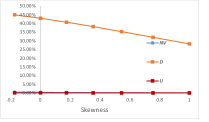
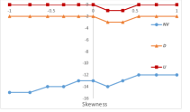
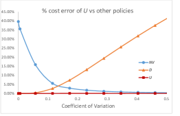
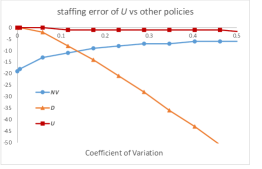
Figure 6.1 plots the relative percentage cost error and staffing error of U๐‘ˆU, Nโ€‹V๐‘๐‘‰NV and D๐ทD. The staffing error and percentage cost error for U๐‘ˆU is defined as in columns seven and eight in Table 6.1, and is defined similarly for D๐ทD and Nโ€‹V๐‘๐‘‰NV. Table B.1 in EC contains further details regarding this study, such as the exact costs and staffing levels. We see from Figure 6.1 that U๐‘ˆU staffs very close to the optimal staffing level and therefore performs well even for very high CV values. We also see that U๐‘ˆU outperforms Nโ€‹V๐‘๐‘‰NV for lower CV values and outperforms D๐ทD for higher CV values. Furthermore, in both cases, the staffing and percentage cost error can be arbitrarily large. Hence we conclude that U๐‘ˆU is robust and performs extremely well even in parameter settings beyond which it has been proven to be asymptotically optimal.
Refer to caption
(a) % cost error
Refer to caption
(b) staffing error (i.e., Noptโˆ’โ–ณsuperscript๐‘optโ–ณN^{\mbox{\tiny{opt}}}-\triangle where โ–ณโˆˆ{NU,ND,NNโ€‹V}โ–ณsubscript๐‘๐‘ˆsubscript๐‘๐ทsubscript๐‘๐‘๐‘‰\triangle\in\{N_{U},N_{D},N_{NV}\})
Figure 6.1: Performance of U๐‘ˆU and other policies for increasing CV

Figure 6.1 is a first step in concluding that U๐‘ˆU is very robust, and performs extremely well over a large range of parameter settings much beyond where Theorems 1 and 2 establish its asymptotic optimality. The next step in establishing the aforementioned conclusion is to explore the effect of varying other parameters, for example the staffing cost.

6.3 Varying Staffing Costs

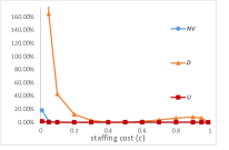
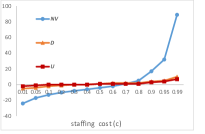
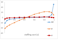
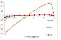
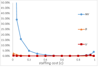
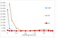
Next, we explore the effect of the staffing cost, which determines the associated critical ratio of the newsvendor policy. To do this, we change the staffing cost c๐‘c while holding the other parameters constant. We perform three separate studies by fixing the arrival rate distribution at three separate levels of uncertainty; low CV, moderate CV and high CV. In particular, we assume ฮ›โˆผ๐’ฐโ€‹[90,110]similar-toฮ›๐’ฐ90110\Lambda\sim\mathcal{U}[90,110] to produce low CV (Figures 6.2a and 6.3a), ฮ›โˆผ๐’ฐโ€‹[50,150]similar-toฮ›๐’ฐ50150\Lambda\sim\mathcal{U}[50,150] to produce moderate CV (Figures 6.2b and 6.3b), and ฮ›โˆผ๐’ฐโ€‹[10,190]similar-toฮ›๐’ฐ10190\Lambda\sim\mathcal{U}[10,190] to produce high CV (Figures 6.2c and 6.3c). We plot the percentage cost errors in Figure 6.2 and the staffing errors in Figure 6.3 for U๐‘ˆU, D๐ทD and Nโ€‹V๐‘๐‘‰NV. We refer the reader to Tables B.2-B.4 in EC for further details (exact costs and staffing levels).
Refer to caption
(a) low CV (Cโ€‹Vฮ›=0.0144๐ถsubscript๐‘‰ฮ›0.0144CV_{\Lambda}=0.0144)
Refer to caption
(b) moderate CV (Cโ€‹Vฮ›=0.0722๐ถsubscript๐‘‰ฮ›0.0722CV_{\Lambda}=0.0722)
Refer to caption
(c) high CV (Cโ€‹Vฮ›=0.1299๐ถsubscript๐‘‰ฮ›0.1299CV_{\Lambda}=0.1299)
Figure 6.2: % cost error for changing staffing costs at three levels of arrival rate uncertainty
Refer to caption
(a) low CV (Cโ€‹Vฮ›=0.0144๐ถsubscript๐‘‰ฮ›0.0144CV_{\Lambda}=0.0144)
Refer to caption
(b) moderate CV (Cโ€‹Vฮ›=0.0722๐ถsubscript๐‘‰ฮ›0.0722CV_{\Lambda}=0.0722)
Refer to caption
(c) high CV (Cโ€‹Vฮ›=0.1299๐ถsubscript๐‘‰ฮ›0.1299CV_{\Lambda}=0.1299)
Figure 6.3: staffing error (i.e., Noptโˆ’โ–ณsuperscript๐‘optโ–ณN^{\mbox{\tiny{opt}}}-\triangle where โ–ณโˆˆ{NU,ND,NNโ€‹V}โ–ณsubscript๐‘๐‘ˆsubscript๐‘๐ทsubscript๐‘๐‘๐‘‰\triangle\in\{N_{U},N_{D},N_{NV}\}) for changing staffing costs at three levels of arrival rate uncertainty

We first observe that for all staffing costs and across all levels of CV, U๐‘ˆU staffs very close to the optimal policy and thus performs extremely well. On the other hand, Nโ€‹V๐‘๐‘‰NV performs poorly when the staffing cost is low although the effect gets less pronounced for higher CV values. This is because Nโ€‹V๐‘๐‘‰NV tends to understaff for low staffing costs when the CV is low. As a result, when cโ‰ชp<amuch-less-than๐‘๐‘๐‘Žc\ll p<a, Nโ€‹V๐‘๐‘‰NV incurs higher routing control and abandonment costs. As the in-house staffing cost c๐‘c increases to p=1๐‘1p=1, Nโ€‹V๐‘๐‘‰NV tends to overstaff, although the adverse effects of overstaffing are not as detrimental. We see that D๐ทD performs very poorly as the CV level increases because it fails to capture the effect of randomness. Overall, we see that U๐‘ˆU is robust and performs well across different critical ratio and CV combinations while the alternative policies can perform arbitrarily poorly.

6.4 Effect of distribution asymmetry

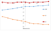
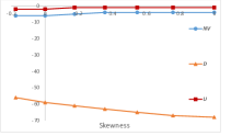
Our numerical result thus far have assumed symmetric Uniform arrival rate distributions. Next, we generalize our results by considering arrival rate distributions that are asymmetric and follow a Beta distribution to study the effect of skewness on the performance of U๐‘ˆU and the other policies. Specifically, we assume that ฮ›โˆผBโ€‹eโ€‹tโ€‹aโ€‹(ฮฑ1,ฮฑ2,ฮปโˆ’bยฏโ€‹ฮป,ฮป+bยฏโ€‹ฮป)similar-toฮ›๐ต๐‘’๐‘ก๐‘Žsubscript๐›ผ1subscript๐›ผ2๐œ†ยฏ๐‘๐œ†๐œ†ยฏ๐‘๐œ†\Lambda\sim Beta(\alpha_{1},\alpha_{2},\lambda-\underline{b}\sqrt{\lambda},\lambda+\overline{b}\sqrt{\lambda}), where the first two arguments are the scale parameters of the distribution and the last two arguments are the lower and upper bounds of the support. We let bยฏยฏ๐‘\underline{b} and bยฏยฏ๐‘\overline{b} be arbitrarily large so that the arrival rate may not realize in the QED regime (i.e., the assumptionย 4.1 is not necessarily satisfied). Our proposed policy U๐‘ˆU is defined for XโˆผBโ€‹eโ€‹tโ€‹aโ€‹(ฮฑ1,ฮฑ2,bยฏ,bยฏ)similar-to๐‘‹๐ต๐‘’๐‘ก๐‘Žsubscript๐›ผ1subscript๐›ผ2ยฏ๐‘ยฏ๐‘X\sim Beta(\alpha_{1},\alpha_{2},\underline{b},\overline{b}) from (5.1).

We keep the mean arrival rate fixed at Eโ€‹[ฮ›]=ฮป=100๐ธdelimited-[]ฮ›๐œ†100E[\Lambda]=\lambda=100 (i.e., Eโ€‹[X]=0๐ธdelimited-[]๐‘‹0E[X]=0) throughout this section and we consider three cases where we keep the variance of the arrival rate fixed at three levels: The low CV case keeps the variance of ฮ›ฮ›\Lambda fixed and equal to that of a ๐’ฐโ€‹[90,110]๐’ฐ90110\mathcal{U}[90,110] random variable (i.e., Vโ€‹aโ€‹rโ€‹(X)=Vโ€‹aโ€‹rโ€‹(๐’ฐโ€‹[โˆ’1,1])๐‘‰๐‘Ž๐‘Ÿ๐‘‹๐‘‰๐‘Ž๐‘Ÿ๐’ฐ11Var\left(X\right)=Var\left(\mathcal{U}\left[-1,1\right]\right)), the moderate CV case keeps the variance of ฮ›ฮ›\Lambda fixed and equal to that of a ๐’ฐโ€‹[50,150]๐’ฐ50150\mathcal{U}[50,150] random variable (i.e., Vโ€‹aโ€‹rโ€‹(X)=Vโ€‹aโ€‹rโ€‹(๐’ฐโ€‹[โˆ’5,5])๐‘‰๐‘Ž๐‘Ÿ๐‘‹๐‘‰๐‘Ž๐‘Ÿ๐’ฐ55Var\left(X\right)=Var\left(\mathcal{U}\left[-5,5\right]\right)), and the high CV case keeps the variance of ฮ›ฮ›\Lambda fixed and equal to that of a ๐’ฐโ€‹[10,190]๐’ฐ10190\mathcal{U}[10,190] random variable (i.e., Vโ€‹aโ€‹rโ€‹(X)=Vโ€‹aโ€‹rโ€‹(๐’ฐโ€‹[โˆ’9,9])๐‘‰๐‘Ž๐‘Ÿ๐‘‹๐‘‰๐‘Ž๐‘Ÿ๐’ฐ99Var\left(X\right)=Var\left(\mathcal{U}\left[-9,9\right]\right)).

We study the effect of asymmetry by changing the skewness of the Beta distribution through its scale parameters ฮฑ1subscript๐›ผ1\alpha_{1} and ฮฑ2subscript๐›ผ2\alpha_{2}. In particular, we set Eโ€‹[X]=ฮฑ1โ€‹bยฏ+ฮฑ2โ€‹bยฏฮฑ1+ฮฑ2=0๐ธdelimited-[]๐‘‹subscript๐›ผ1ยฏ๐‘subscript๐›ผ2ยฏ๐‘subscript๐›ผ1subscript๐›ผ20E[X]=\frac{\alpha_{1}\overline{b}+\alpha_{2}\underline{b}}{\alpha_{1}+\alpha_{2}}=0 and Vโ€‹aโ€‹rโ€‹(X)=ฮฑ1โ€‹ฮฑ2โ€‹(bยฏโˆ’bยฏ)2(ฮฑ1+ฮฑ2)2โ€‹(ฮฑ1+ฮฑ2+1)=ฯƒ2๐‘‰๐‘Ž๐‘Ÿ๐‘‹subscript๐›ผ1subscript๐›ผ2superscriptยฏ๐‘ยฏ๐‘2superscriptsubscript๐›ผ1subscript๐›ผ22subscript๐›ผ1subscript๐›ผ21superscript๐œŽ2Var\left(X\right)=\frac{\alpha_{1}\alpha_{2}\left(\overline{b}-\underline{b}\right)^{2}}{\left(\alpha_{1}+\alpha_{2}\right)^{2}\left(\alpha_{1}+\alpha_{2}+1\right)}=\sigma^{2}, where ฯƒ2superscript๐œŽ2\sigma^{2} denotes the variance of the associated CV level, and we choose555Note that setting Eโ€‹[X]=0๐ธdelimited-[]๐‘‹0E[X]=0 yields bยฏbยฏ=โˆ’ฮฑ2ฮฑ1ยฏ๐‘ยฏ๐‘subscript๐›ผ2subscript๐›ผ1\frac{\overline{b}}{\underline{b}}=-\frac{\alpha_{2}}{\alpha_{1}}, which together with Var(X))=ฯƒ2Var\left(X\right))=\sigma^{2} yields bยฏ2=ฯƒ2โ€‹ฮฑ1โ€‹(ฮฑ1+ฮฑ2+1)ฮฑ2superscriptยฏ๐‘2superscript๐œŽ2subscript๐›ผ1subscript๐›ผ1subscript๐›ผ21subscript๐›ผ2\underline{b}^{2}=\frac{\sigma^{2}\alpha_{1}(\alpha_{1}+\alpha_{2}+1)}{\alpha_{2}}. Hence the values of ฮฑ1subscript๐›ผ1\alpha_{1}, ฮฑ2subscript๐›ผ2\alpha_{2}, bยฏยฏ๐‘\underline{b}, and bยฏยฏ๐‘\overline{b} are not fully determined and we arbitrarily set ฮฑ1+ฮฑ2=2subscript๐›ผ1subscript๐›ผ22\alpha_{1}+\alpha_{2}=2 and change ฮฑ1subscript๐›ผ1\alpha_{1} and ฮฑ2subscript๐›ผ2\alpha_{2} accordingly, which also changes bยฏยฏ๐‘\underline{b} and bยฏยฏ๐‘\overline{b}. ฮฑ1subscript๐›ผ1\alpha_{1} and ฮฑ2subscript๐›ผ2\alpha_{2} such that ฮฑ1+ฮฑ2=2subscript๐›ผ1subscript๐›ผ22\alpha_{1}+\alpha_{2}=2. We start with a negative-skewed (left-skewed) Beta distribution with scale parameters ฮฑ1=1.5subscript๐›ผ11.5\alpha_{1}=1.5 and ฮฑ2=0.5subscript๐›ผ20.5\alpha_{2}=0.5 with a corresponding skewness of โˆ’11-1. Then we decrease ฮฑ1subscript๐›ผ1\alpha_{1} and increase ฮฑ2subscript๐›ผ2\alpha_{2} so that the skewness of the Beta distribution increases.666Recall that the skewness of Beta distribution is given by 2โ€‹(ฮฑ2โˆ’ฮฑ1)โ€‹(ฮฑ1+ฮฑ2+1)(ฮฑ1+ฮฑ2+2)โ€‹(ฮฑ1โ€‹ฮฑ2)2subscript๐›ผ2subscript๐›ผ1subscript๐›ผ1subscript๐›ผ21subscript๐›ผ1subscript๐›ผ22subscript๐›ผ1subscript๐›ผ2\frac{2(\alpha_{2}-\alpha_{1})(\sqrt{\alpha_{1}+\alpha_{2}+1})}{(\alpha_{1}+\alpha_{2}+2)(\sqrt{\alpha_{1}\alpha_{2}})}. The mid-point where ฮฑ1=ฮฑ2=1subscript๐›ผ1subscript๐›ผ21\alpha_{1}=\alpha_{2}=1 and so the skewness equals 0, corresponds to the symmetric Uniform distribution. After ฮฑ1=ฮฑ2=1subscript๐›ผ1subscript๐›ผ21\alpha_{1}=\alpha_{2}=1, the distribution becomes positive-skewed (right-skewed) as we decrease ฮฑ1subscript๐›ผ1\alpha_{1} and increase ฮฑ2subscript๐›ผ2\alpha_{2} and we continue until ฮฑ1=0.5subscript๐›ผ10.5\alpha_{1}=0.5 and ฮฑ2=1.5subscript๐›ผ21.5\alpha_{2}=1.5 which corresponds to a skewness of +11+1. We plot the percentage cost error and staffing errors of U๐‘ˆU and the other policies in Figure 6.4 and Figure 6.5, respectively. Tables B.6-B.8 in EC provide further details (the exact costs and staffing levels as well as the shape parameters of the Beta distribution).
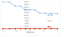
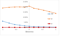
Refer to caption
(a) low CV (Cโ€‹Vฮ›=0.0144๐ถsubscript๐‘‰ฮ›0.0144CV_{\Lambda}=0.0144)
Refer to caption
(b) moderate CV (Cโ€‹Vฮ›=0.0722๐ถsubscript๐‘‰ฮ›0.0722CV_{\Lambda}=0.0722)
Refer to caption
(c) high CV (Cโ€‹Vฮ›=0.1299๐ถsubscript๐‘‰ฮ›0.1299CV_{\Lambda}=0.1299)
Figure 6.4: % cost error for varying skewness levels at three levels of arrival rate uncertainty
Refer to caption
(a) low CV (Cโ€‹Vฮ›=0.0144๐ถsubscript๐‘‰ฮ›0.0144CV_{\Lambda}=0.0144)
Refer to caption
(b) moderate CV (Cโ€‹Vฮ›=0.0722๐ถsubscript๐‘‰ฮ›0.0722CV_{\Lambda}=0.0722)
Refer to caption
(c) high CV (Cโ€‹Vฮ›=0.1299๐ถsubscript๐‘‰ฮ›0.1299CV_{\Lambda}=0.1299)
Figure 6.5: staffing error (i.e., Noptโˆ’โ–ณsuperscript๐‘optโ–ณN^{\mbox{\tiny{opt}}}-\triangle where โ–ณโˆˆ{NU,ND,NNโ€‹V}โ–ณsubscript๐‘๐‘ˆsubscript๐‘๐ทsubscript๐‘๐‘๐‘‰\triangle\in\{N_{U},N_{D},N_{NV}\}) for varying skewness at three levels of arrival rate uncertainty

From Figure 6.4 and Figure 6.5, we first see that U๐‘ˆU continues to perform well under asymmetric arrival rate distributions and across varying levels of skewness. In line with our observations for the uniform distribution, D๐ทD does not perform well except for low CV values. On the other hand, the newsvendor policy performs well for high levels of variability while its performance deteriorates for lower levels of variability and in particular left-skewed distribution. This is because the newsvendor staffing is given by NNโ€‹V:=ฮป+ฮฒ2โ‹†โ€‹ฮปassignsubscript๐‘๐‘๐‘‰๐œ†superscriptsubscript๐›ฝ2โ‹†๐œ†N_{NV}:=\lambda+\beta_{2}^{\star}\sqrt{\lambda} for ฮฒ2โ‹†:=FXโˆ’1โ€‹(pโˆ’cp)assignsuperscriptsubscript๐›ฝ2โ‹†superscriptsubscript๐น๐‘‹1๐‘๐‘๐‘\beta_{2}^{\star}:=F_{X}^{-1}(\frac{p-c}{p}), which decreases as the skewness decreases. Hence, the newsvendor staffs less as skewness decreases and the distribution gets more left-skewed, as seen in Figure 6.5. Therefore the newsvendor performs worse when the distribution is left-skewed because its understaffing is more severe, resulting in higher abandonment and routing control costs.

6.5 Discussion

Our numerical results in Sections 6.1 - 6.4 show that U๐‘ˆU is extremely robust, and achieves close to minimum cost over a large range of parameters and assumptions on the amount of the arrival rate uncertainty, and its distribution form. In fact, in virtually all of our experiments U๐‘ˆU outperformed D๐ทD and Nโ€‹V๐‘๐‘‰NV and achieved a cost that was very close to the true optimal cost. To better understand the reason for the extremely robust performance of U๐‘ˆU, we compare the actual expected cost to the diffusion approximation of the expected cost, for a wide range of staffing levels. We keep the staffing level N๐‘N fixed, and approximate the cost using the expression that appears in the limit in Theoremย 1. However, we do not assume that the form of the arrival rate uncertainty is consistent with (4.1) (as assumed by Theoremย 1). Specifically, for

ฮฒ=Nโˆ’ฮปฮปโ€‹ย andย โ€‹X=ฮ›โˆ’ฮปฮป,๐›ฝ๐‘๐œ†๐œ†ย andย ๐‘‹ฮ›๐œ†๐œ†\beta=\frac{N-\lambda}{\sqrt{\lambda}}\mbox{ and }X=\frac{\Lambda-\lambda}{\sqrt{\lambda}},

it follows that the limiting diffusion cost cโ€‹ฮฒ+Eโ€‹[z^โ€‹(ฮฒโˆ’X,T^โ‹†โ€‹(ฮฒโˆ’X))]๐‘๐›ฝ๐ธdelimited-[]^๐‘ง๐›ฝ๐‘‹superscript^๐‘‡โ‹†๐›ฝ๐‘‹c\beta+E\left[\hat{z}(\beta-X,\hat{T}^{\star}(\beta-X))\right] when re-scaled gives the following approximation for the actual cost:

cโ€‹N+Eโ€‹[zoptโ€‹(N,ฮ›)]๐‘๐‘๐ธdelimited-[]superscript๐‘งopt๐‘ฮ›\displaystyle cN+E\left[z^{\mbox{\tiny{opt}}}\left(N,\Lambda\right)\right] โ‰ˆ\displaystyle\approx cโ€‹ฮป+ฮปโ€‹(cโ€‹ฮฒ+Eโ€‹[z^โ€‹(ฮฒโˆ’X,T^โ‹†โ€‹(ฮฒโˆ’X))])๐‘๐œ†๐œ†๐‘๐›ฝ๐ธdelimited-[]^๐‘ง๐›ฝ๐‘‹superscript^๐‘‡โ‹†๐›ฝ๐‘‹\displaystyle c\lambda~{}+~{}\sqrt{\lambda}\left(c\beta+E\left[\hat{z}(\beta-X,\hat{T}^{\star}(\beta-X))\right]\right) (6.2)
=\displaystyle= cโ€‹N+ฮปโ€‹Eโ€‹[z^โ€‹(ฮฒโˆ’X,T^โ‹†โ€‹(ฮฒโˆ’X))].๐‘๐‘๐œ†๐ธdelimited-[]^๐‘ง๐›ฝ๐‘‹superscript^๐‘‡โ‹†๐›ฝ๐‘‹\displaystyle cN+\sqrt{\lambda}E\left[\hat{z}(\beta-X,\hat{T}^{\star}(\beta-X))\right].

Figureย 6.6 demonstrates numerically that the approximation (6.2) is very accurate, far beyond what is proven in Theoremย 1. Specifically, Figureย 6.6 plots the actual expected cost (the left-hand side of (6.2)) and the re-scaled diffusion cost (the right-hand side of (6.2)), and the difference between the two. It is clear that the approximation in (6.2) is extremely accurate, over a wide range of staffing levels. This helps explain the robustness in the performance of U๐‘ˆU.

Figureย 6.6 suggests that the performance of square root safety staffing policies can be approximated well without making special assumptions on the limit regime; that is, there is a โ€œuniversalโ€ approximation. This is because we do not restrict ฮฒ๐›ฝ\beta values to a particular range which can also be evidenced from the ฮฒโ‹†superscript๐›ฝโ‹†\beta^{\star} values that we observed in our numerical studies in Sectionsย 6.1-6.4. In particular, the ฮฒโ‹†superscript๐›ฝโ‹†\beta^{\star} values in Figures 2-4 come from a wide range from -12 to 10 (see Table B.5 for details). Recalling that ฮป=10๐œ†10\sqrt{\lambda}=10 in Figures 2-4, we observe that such extremely low or high values of ฮฒโ‹†superscript๐›ฝโ‹†\beta^{\star} that are essentially of the same order of magnitude as ฮป๐œ†\sqrt{\lambda} (so that the resulting safety staffing is in fact of order ฮป๐œ†\lambda) allow us to capture heavily overloaded or underloaded systems, and thus allows us to approximate parameter regimes beyond what is assumed in our asymptotic analysis in Section 4.

Our observation is also consistent with the universal approximation result of Gurvich etย al. (2013) for a M/M/N+M model with deterministic arrival rate and no routing control. Although it is tempting to think that Gurvich etย al. (2013) can be used to explain Figureย 6.6, the modeling generalization from a deterministic to a random arrival rate is not immediate, even if we do not allow for outsourcing. Our goal is to show that

Eโ€‹[zฯ„โ€‹(โˆž)โ€‹(N,ฮ›)]โˆ’ฮปโ€‹Eโ€‹[z^โ€‹(Nโˆ’ฮ›ฮป,โˆž)]=๐’ชโ€‹(1),๐ธdelimited-[]subscript๐‘ง๐œ๐‘ฮ›๐œ†๐ธdelimited-[]^๐‘ง๐‘ฮ›๐œ†๐’ช1E\left[z_{\tau(\infty)}(N,\Lambda)\right]-\sqrt{\lambda}E\left[\hat{z}\left(\frac{N-\Lambda}{\sqrt{\lambda}},\infty\right)\right]=\mathcal{O}(1), (6.3)

where z^โ€‹(m,โˆž)^๐‘ง๐‘š\hat{z}(m,\infty) is as defined in Lemmaย 1, when the limit as T^โ†’โˆžโ†’^๐‘‡\hat{T}\rightarrow\infty is taken. Under the policy ฯ„โ€‹(โˆž)๐œ\tau(\infty) that outsources no customers (and so besides staffing only incurs costs through customer abandonment), then zฯ„โ€‹(โˆž)โ€‹(N,l)=aโ€‹ฮณโ€‹Qยฏฯ„โ€‹(โˆž)โ€‹(l)subscript๐‘ง๐œ๐‘๐‘™๐‘Ž๐›พsubscriptยฏ๐‘„๐œ๐‘™z_{\tau(\infty)}(N,l)=a\gamma\overline{Q}_{\tau(\infty)}(l), and so it follows from Corollary 1 in Gurvich etย al. (2013) and algebraic manipulation that

zฯ„โ€‹(โˆž)โ€‹(N,l)โˆ’lโ€‹z^โ€‹(Nโˆ’ll,โˆž)=๐’ชโ€‹(1).subscript๐‘ง๐œ๐‘๐‘™๐‘™^๐‘ง๐‘๐‘™๐‘™๐’ช1z_{\tau(\infty)}(N,l)-\sqrt{l}\hat{z}\left(\frac{N-l}{\sqrt{l}},\infty\right)=\mathcal{O}(1). (6.4)

Although it seems reasonable that a technical argument would enable us to show that (6.4) implies

Eโ€‹[zฯ„โ€‹(โˆž)โ€‹(N,ฮ›)]โˆ’Eโ€‹[ฮ›โ€‹z^โ€‹(Nโˆ’ฮ›ฮ›,โˆž)]=๐’ชโ€‹(1),๐ธdelimited-[]subscript๐‘ง๐œ๐‘ฮ›๐ธdelimited-[]ฮ›^๐‘ง๐‘ฮ›ฮ›๐’ช1E\left[z_{\tau(\infty)}(N,\Lambda)\right]-E\left[\sqrt{\Lambda}\hat{z}\left(\frac{N-\Lambda}{\sqrt{\Lambda}},\infty\right)\right]=\mathcal{O}(1),

it is not clear how to establish that

ฮปโ€‹Eโ€‹[z^โ€‹(Nโˆ’ฮ›ฮป,โˆž)]โˆ’Eโ€‹[ฮ›โ€‹z^โ€‹(Nโˆ’ฮ›ฮ›,โˆž)]=๐’ชโ€‹(1),๐œ†๐ธdelimited-[]^๐‘ง๐‘ฮ›๐œ†๐ธdelimited-[]ฮ›^๐‘ง๐‘ฮ›ฮ›๐’ช1\sqrt{\lambda}E\left[\hat{z}\left(\frac{N-\Lambda}{\sqrt{\lambda}},\infty\right)\right]-E\left[\sqrt{\Lambda}\hat{z}\left(\frac{N-\Lambda}{\sqrt{\Lambda}},\infty\right)\right]=\mathcal{O}(1), (6.5)

Intuitively, we expect something like (6.5) to be true because as the system becomes more understaffed z^โ€‹(โ‹…,โˆž)^๐‘งโ‹…\hat{z}(\cdot,\infty) starts to look linear and as the system becomes more overstaffed z^โ€‹(โ‹…,โˆž)^๐‘งโ‹…\hat{z}(\cdot,\infty) should be negligible (and when the staffing is neither severely understaffed or overstaffed we can appeal to Theoremย 1). However, the analytic argument is not straightforward, and remains as an open question.
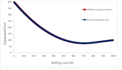
Refer to caption
(a)
Refer to caption
(b)
Figure 6.6: Expected Cost Difference: Actual vs Diffusion. [ฮ›โˆผ๐’ฐโ€‹[20,780]similar-toฮ›๐’ฐ20780\Lambda\sim\mathcal{U}[20,780], ฮป=400๐œ†400\lambda=400, c=0.1๐‘0.1c=0.1, p=1๐‘1p=1 and a=5๐‘Ž5a=5.]

7 Conclusions

Customer call centers face the difficult challenge of having to determine staffing levels in the face of a high level of variability in customer demand. Making these upfront decisions may result in either over- or under-staffing, which implies large unnecessary operating costs. One strategy that call centers use to mitigate these risks is to co-source. Then there is a dynamic decision of whether to handle an arriving call in-house or to outsource it. Our paper deals with the joint staffing and dynamic outsourcing decision for a co-sourced customer call center. The key feature in our model is the time scales differentiation, where staffing decisions are made upfront when the arrival rate is uncertain, while the outsourcing decisions are made dynamically in real-time with full knowledge of the arrival rate realization as well as the system state.

We propose the policy U๐‘ˆU, which staffs the center with the mean offered load plus a safety staffing that is of the order of square root of this mean offered load. The policy also outsources calls whenever the number of customers in line exceeds a threshold. When the order of magnitude of arrival rate randomness is the same order as the inherent system fluctuations in the queue length (which is on the order of the square root of the realized arrival rate), we show that our proposed policy is asymptotically optimal as the mean arrival rate grows large. Then, we perform an extensive numerical experiment to study the performance of U๐‘ˆU beyond the regime for which it is proved to be asymptotically optimal. In all of our numerical experiments in which the system has more than a few servers we did not encounter even one case in which the performance of U๐‘ˆU was not superb. In contrast, our two benchmark policies each have parameter regimes in which their performance can be arbitrarily bad. It is, therefore, the robustness of the performance of U๐‘ˆU that we would like to stress as the main takeaway from this paper. One does not need to identify the โ€œrightโ€ operating regime in order to determine which policy to use. The U๐‘ˆU policy appears to be a โ€œone-size-fits-allโ€.

We further observe from our numerical results that the newsvendor policy performs well except when the in-house staffing cost c๐‘c is low relative to the costs of outsourcing p๐‘p and abandonment a๐‘Ža. Since the newsvendor policy is a simpler policy than U๐‘ˆU, the question arises: can we use the newsvendor instead of U๐‘ˆU? Although the answer is โ€œyesโ€ for a non-trivial portion of the parameter space, the answer is โ€œnoโ€ when considering the entire parameter space. This is important because outsourcing costs can be very high when the hidden costs of outsourcing are included (Kharif, 2003) and (Rubin, 2013). A recent study (InfoTech, 2011) shows that โ€œhidden costsโ€ of outsourcing add, on average, 25% to the overall cost showing that the hidden costs of outsourcing can indeed be significant.

Several important extensions are worth pursuing. In this paper, the recourse action we consider, in case the center is under-staffed is outsourcing some calls to an outside vendor (other actions have been considered in the literature such as utilizing โ€œon-callโ€ agents, Mehrotra etย al. (2010), Gans etย al. (2012), or by sharing resources with other sitesย Perry and Whitt (2009)). On the flip side, one might consider recourse actions for scenarios in which the call center ends up being over-staffed. Those may include sending agents home (as in Mehrotra etย al. (2010), Gans etย al. (2012)) or, if this is not desirable or feasible, diverting agents to other activities such as making outbound calls (Gans and Zhou (2007); Bhulai and Koole (2003)) or cross-selling (Gurvich etย al. (2000); Armony and Gurvich (2010)). It would be interesting to examine a framework in which recourse actions in both directions may be used.

Another interesting extension is to model the staffing decisions of the outside vendor more explicitly, as in Gurvich and Perry (2012) in the case of known arrival rate. In our model we assume that a call outsourced incurs a fixed cost no matter how many calls are sent to the outside vendor. This is consistent with the assumption made in AkลŸin etย al. (2008), and is equivalent to assuming either that the outside service provider has ample service capacity or that it pools demand from a large enough client base so that the calls the company sends to the outside vendor do not have much impact. For the case where the outsourcing is not preferred or does not exist, we see that the performance of U๐‘ˆU remains superb. (We do not report these results due to space limitations.) However, if the outsourcing capacity is positive and limited we do not know how U๐‘ˆU will perform, or how it would need to be modified to maintain this superior performance.

The aforementioned performance deterioration may be mitigated by designing contracts that ensure the outside vendor has ample capacity. But is such a design optimal? It would be interesting to incorporate arrival rate uncertainty when studying contract design questions such as those studied in AkลŸin etย al. (2008), and Zhou and Ren (2011).

Beyond the co-sourcing application considered in this paper, one might use a similar framework to examine joint staffing and control decisions with other system topologies and other types of control such as the problems considered inย Gurvich etย al. (2008),ย Dai and Tezcan (2008),ย Tezcan and Dai (2010),ย Gurvich and Whitt (2010), andย Armony and Mandelbaum (2011). In particular, it will sometimes be possible to incorporate arrival rate uncertainty without changing the control that has been proven to be asymptotically optimal when the arrival rate is known. Ideally, the robustness of the policy performance with respect to the assumptions on the arrival rate uncertainty in this model will be true in much more generality. Skill-based routing is one particularly interesting direction, where not only does one have to determine the size of multiple pools of agents under arrival rate uncertainty, but also, once the arrival rate is known, dynamic control is used to determine the assignment of calls to agents. This setting raises another interesting modeling question that has to do with how to model the arrival rate uncertainty in the presence of multiple streams of arrivals (Shen and Huang (2008), Ibrahim and Lโ€™Ecuyer (2013)).

Finally, our numerical results with respect to the remarkable robustness of U๐‘ˆU suggest that there might be an underlying theoretical justification to this robustness, in the spirit of the universal approximation of Gurvich etย al. (2013). In Section 6.5 we have discussed why their results in a framework that assumes a known arrival rate and no dynamic control may not be readily applied to our framework. But one wonders whether similar universal approximation principles apply when a random arrival rate and dynamic control are incorporated into the model.

\c@NAT@ctr

References

  • Aksin etย al. (2007) Aksin, Z., M.ย Armony, V.ย Mehrotra. 2007. The modern call center: A multi-disciplinary perspective on operations management research. Production and Operations Management 16(6) 665โ€“688.
  • AkลŸin etย al. (2008) AkลŸin, Z., F.ย deย Vรฉricourt, F.ย Karaesmen. 2008. Call center outsourcing contract analysis and choice. Management Science 54(2) 354โ€“368.
  • Armony and Gurvich (2010) Armony, M., I.ย Gurvich. 2010. When promotions meet operations: Cross selling and its effect on call-center performance. Manufacturing & Service Operations Management 12(3) 470โ€“488.
  • Armony and Mandelbaum (2011) Armony, M., A.ย Mandelbaum. 2011. Routing and staffing in large-scale service systems: The case of homogeneous impatient customers and heterogeneous servers. Operations research 59(1) 50โ€“65.
  • Armony etย al. (2009) Armony, M., E.ย Plambeck, S.ย Seshadri. 2009. Sensitivity of optimal capacity to customer impatience in an unobservable m/m/s queue (why you shouldnโ€™t shout at the dmv). Manufacturing & Service Operations Management 11(1) 19โ€“32.
  • Bassamboo etย al. (2005) Bassamboo, A., J.M. Harrison, A.ย Zeevi. 2005. Dynamic routing and admission control in high-volume service systems: Asymptotic analysis via multi-scale fluid limits. Queueing Systems 51(3) 249โ€“285.
  • Bassamboo etย al. (2006) Bassamboo, A., J.M. Harrison, A.ย Zeevi. 2006. Design and Control of a Large Call Center: Asymptotic Analysis of an LP-Based Method. Operations Research 54(3) 419โ€“435.
  • Bassamboo etย al. (2010) Bassamboo, A., R.S. Randhawa, A.ย Zeevi. 2010. Capacity sizing under parameter uncertainty: Safety staffing principles revisited. Management Science 56(10) 1668โ€“1686.
  • Bassamboo and Zeevi (2009) Bassamboo, A., A.ย Zeevi. 2009. On a Data-Driven Method for Staffing Large Call Centers. Operations Research 57(3) 714โ€“726.
  • Bhulai and Koole (2003) Bhulai, S., G.ย Koole. 2003. A queueing model for call blending in call centers. IEEE transactions on automatic control 48 1434โ€“1438.
  • Borst etย al. (2004) Borst, S., A.ย Mandelbaum, M.I. Reiman. 2004. Dimensioning large call centers. Operations research 52(1) 17โ€“34.
  • Brown etย al. (2005) Brown, L., N.ย Gans, A.ย Mandelbaum, A.ย Sakov, H.ย Shen, S.ย Zeltyn, L.ย Zhao. 2005. Statistical Analysis of a Telephone Call Center. Journal of the American Statistical Association 100(469) 36โ€“50.
  • Chen and Henderson (2001) Chen, B.P.K., S.G. Henderson. 2001. Two issues in setting call centre staffing levels. Annals of Operations Research 108(1) 175โ€“192.
  • Dai and Tezcan (2008) Dai, J.G., T.ย Tezcan. 2008. Optimal control of parallel server systems with many servers in heavy traffic. Queueing Systems 59 95โ€“134.
  • Gans etย al. (2003) Gans, N., G.ย Koole, A.ย Mandelbaum. 2003. Telephone call centers: Tutorial, review, and research prospects. Manufacturing & Service Operations Management 5(2) 79โ€“141.
  • Gans etย al. (2012) Gans, N., H.ย Shen, Y-P Zhou, K.ย Korolev, A.ย McCord, H.ย Ristock. 2012. Parametric stochastic programming models for call-center workforce scheduling. Working Paper.
  • Gans and Zhou (2007) Gans, N., Y.P. Zhou. 2007. Call-routing schemes for call-center outsourcing. Manufacturing & Service Operations Management 9(1) 33โ€“50.
  • Garnett etย al. (2002) Garnett, O., A.ย Mandelbaum, M.ย Reiman. 2002. Designing a call center with impatient customers. Manufacturing & Service Operations Management 4(3) 208โ€“227.
  • Gilson and Khandelwal (2005) Gilson, K.ย A., D.ย K. Khandelwal. 2005. Getting more from call centers. The McKinsey Quaterly.
  • Green etย al. (2001) Green, L.V., P.J. Kolesar, J.ย Soares. 2001. Improving the sipp approach for staffing service systems that have cyclic demands. Operations Research 49(4) 549โ€“564.
  • Gurvich etย al. (2000) Gurvich, I., M.ย Armony, C.ย Maglaras. 2000. Cross-selling in a call center with a heterogeneous customer population. Operations Research 57(2) 299โ€“313.
  • Gurvich etย al. (2008) Gurvich, I., M.ย Armony, A.ย Mandelbaum. 2008. Service-level differentiation in call centers with fully flexible servers. Management Science 54(2) 279โ€“294.
  • Gurvich etย al. (2013) Gurvich, I., J.ย Huang, A.ย Mandelbaum. 2013. Excursion-based universal approximations for the erlang-a queue in steady-state. Mathematics of Operations Research. Forthcoming.
  • Gurvich etย al. (2010) Gurvich, I., J.ย Luedtke, T.ย Tezcan. 2010. Staffing call centers with uncertain demand forecasts: A chance-constrained optimization approach. Management Science 56(7) 1093โ€“1115.
  • Gurvich and Perry (2012) Gurvich, I., O.ย Perry. 2012. Overflow networks: Approximations and implications to call-center outsourcing. Operations Research 60(4) 996โ€“1009.
  • Gurvich and Whitt (2010) Gurvich, I., W.ย Whitt. 2010. Service-level differentiation in many-server service systems via queue-ratio routing. Operations Research 58(2) 316โ€“328.
  • Halfin and Whitt (1981) Halfin, S., W.ย Whitt. 1981. Heavy-traffic limits for queues with many exponential servers. Operations research 29(3) 567โ€“588.
  • Ibrahim and Lโ€™Ecuyer (2013) Ibrahim, R., P.ย Lโ€™Ecuyer. 2013. Forecasting call center arrivals: Fixed-effects, mixed-effects, and bivariate models. Manufacturing & Service Operations Management 15(1) 72โ€“85.
  • ICMI (2006) ICMI. 2006. ICMIโ€™s Contact Center Outsourcing Report. http://www.icmi.com/files/ICMI/members/ccmr/ccmr2006/ccmr06/June2006_issue.pdf.
  • InfoTech (2011) InfoTech. 2011. Discover the hidden costs of outsourcing. http://www.infotech.com/research/ss/it-discover-the-hidden-costs-of-outsourcing.
  • Jongbloed and Koole (2001) Jongbloed, G., G.ย Koole. 2001. Managing uncertainty in call centres using Poisson mixtures. Applied Stochastic Models in Business and Industry 17(4) 307โ€“318.
  • Kharif (2003) Kharif, O. 2003. The hidden costs of it outsourcing. BusinessWeek (October 26 2003).
  • KoรงaฤŸa and Ward (2010) KoรงaฤŸa, Y.L., A.R. Ward. 2010. Admission Control for a Multi-Server Queue with Abandonment. Queueing Systems 65(3) 275โ€“323.
  • Koole and Pot (2011) Koole, G., A.ย Pot. 2011. A note on profit maximization and monotonicity for inbound call centers. Operations Research 59(5) 1304โ€“1308.
  • Liu and Whitt (2012) Liu, Y., W.ย Whitt. 2012. Stabilizing customer abandonment in many-server queues with time-varying arrivals. Operations Research 60(6) 1551โ€“1564.
  • Maman (2009) Maman, S. 2009. Uncertainty in the demand for service: The case of call centers and emergency departments. Masterโ€™s thesis, Technion-Israel Institute of Technology.
  • Mandelbaum and Zeltyn (2009) Mandelbaum, A., S.ย Zeltyn. 2009. Staffing many-server queues with impatient customers: Constraint satisfaction in call centers. Operations Research 57(5) 1189โ€“1205.
  • Mehrotra etย al. (2010) Mehrotra, V., O.ย Ozlรผk, R.ย Saltzman. 2010. Intelligent procedures for intra-day updating of call center agent schedules. Production and Operations Management 19(3) 353โ€“367.
  • Perry and Whitt (2009) Perry, O., W.ย Whitt. 2009. Responding to unexpected overloads in large-scale service systems. Management Science 55(8) 1353โ€“1367.
  • Robbins and Harrison (2010) Robbins, T.R., T.P. Harrison. 2010. A stochastic programming model for scheduling call centers with global service level agreements. European Journal of Operational Research 207(3) 1608โ€“1619.
  • Ross (2001) Ross, A.M. 2001. Queueing systems with daily cycles and stochastic demand with uncertain parameters. Ph.D. thesis, University of California, Berkeley.
  • Rubin (2013) Rubin, J. 2013. Hidden Costs of Outsourcing. Forbes (March 29). http://www.forbes.com/sites/forbesinsights/2013/03/29/the-hidden-costs-of-outsourcing/.
  • Shen and Huang (2008) Shen, H., J.Z. Huang. 2008. Interday forecasting and intraday updating of call center arrivals. Manufacturing & Service Operations Management 10(3) 391โ€“410.
  • Steckley etย al. (2009) Steckley, S.G., S.G. Henderson, V.ย Mehrotra. 2009. Forecast errors in service systems. Probability in the Engineering and Informational Sciences 23(2) 305โ€“332.
  • Tezcan and Dai (2010) Tezcan, T., J.G. Dai. 2010. Dynamic control of n-systems with many servers: asymptotic optimality of a static priority policy in heavy traffic. Operations Research 58 94โ€“110.
  • Whitt (2005) Whitt, W. 2005. Engineering Solution of a Basic Call-Center Model. Management Science 51(2) 221โ€“235.
  • Whitt (2006) Whitt, W. 2006. Stafffng a Call Center with Uncertain Arrival Rate and Absenteeism. Production and Operations Management 15(1) 88โ€“102.
  • Zan etย al. (2013) Zan, J., J.J. Hasenbein, D.P. Morton. 2013. Staffing large service systems under arrival-rate uncertainty. arXiv preprint arXiv:1304.6701 .
  • Zhou and Ren (2011) Zhou, Y-P., Z.J. Ren. 2011. Service outsourcing. Wiley Encyclopedia of Operations Research and Management Science .

Electronic Companion to โ€œStaffing Call Centers with Uncertain Arrival Rates and Co-sourcingโ€


In this electronic companion, we provide supporting material for our manuscript titled โ€œStaffing Call Centers with Uncertain Arrival Rates and Co-sourcingโ€. We first provide the proofs of the Theorems, Propositions, and Lemmas in the main paper body (Sectionย A) and then provide additional numerical results to support the figures in the main paper body (Sectionย B).

Appendix A Proofs


Proof of Propositionย 1: We first prove part (i) and then prove part (ii).

Proof of part (i): It is helpful to first obtain a lower bound on the cost of any staffing policy, regardless of the routing policy ฯ€โˆˆฮ ๐œ‹ฮ \pi\in\Pi that is followed. For this, let Sยฏฯ€โ€‹(l)subscriptยฏ๐‘†๐œ‹๐‘™\overline{S}_{\pi}(l) be the expected number of busy servers when the arrival rate realization is l๐‘™l, and let Sยฏฯ€โ€‹(ฮ›)subscriptยฏ๐‘†๐œ‹ฮ›\overline{S}_{\pi}(\Lambda) be the associated random variable. Then, since Nโ‰ฅSยฏฯ€โ€‹(l)๐‘subscriptยฏ๐‘†๐œ‹๐‘™N\geq\overline{S}_{\pi}(l),

Cโ€‹(N,ฯ€)โ‰ฅcโ€‹Eโ€‹[Sยฏฯ€โ€‹(ฮ›)]+pโ€‹Eโ€‹[ฮ›โ€‹Pฯ€โ€‹(out;ฮ›)]+aโ€‹Eโ€‹[ฮ›โ€‹Pฯ€โ€‹(ab;ฮ›)],๐ถ๐‘๐œ‹๐‘๐ธdelimited-[]subscriptยฏ๐‘†๐œ‹ฮ›๐‘๐ธdelimited-[]ฮ›subscript๐‘ƒ๐œ‹outฮ›๐‘Ž๐ธdelimited-[]ฮ›subscript๐‘ƒ๐œ‹abฮ›C(N,\pi)\geq cE\left[\overline{S}_{\pi}(\Lambda)\right]+pE\left[\Lambda P_{\pi}(\mbox{out};\Lambda)\right]+aE\left[\Lambda P_{\pi}(\mbox{ab};\Lambda)\right],

so that the assumption cโ‰ฅminโก(a,p)๐‘๐‘Ž๐‘c\geq\min(a,p) then yields

Cโ€‹(N,ฯ€)โ‰ฅminโก(a,p)โ€‹Eโ€‹[Sยฏฯ€โ€‹(ฮ›)+ฮ›โ€‹(Pฯ€โ€‹(out;ฮ›)+Pฯ€โ€‹(ab;ฮ›))].๐ถ๐‘๐œ‹๐‘Ž๐‘๐ธdelimited-[]subscriptยฏ๐‘†๐œ‹ฮ›ฮ›subscript๐‘ƒ๐œ‹outฮ›subscript๐‘ƒ๐œ‹abฮ›C(N,\pi)\geq\min(a,p)E\left[\overline{S}_{\pi}(\Lambda)+\Lambda\left(P_{\pi}(\mbox{out};\Lambda)+P_{\pi}(\mbox{ab};\Lambda)\right)\right]. (A.1)

For any realization l๐‘™l of ฮ›ฮ›\Lambda, the arrival rate into the system must equal the departure rate from the system (due to both abandonments and service completion), so that

lโ€‹(1โˆ’Pฯ€โ€‹(out;l))=Sยฏฯ€โ€‹(l)+lโ€‹Pฯ€โ€‹(ab;l),๐‘™1subscript๐‘ƒ๐œ‹out๐‘™subscriptยฏ๐‘†๐œ‹๐‘™๐‘™subscript๐‘ƒ๐œ‹ab๐‘™l(1-P_{\pi}(\mbox{out};l))=\overline{S}_{\pi}(l)+lP_{\pi}(\mbox{ab};l),

or, equivalently,

l=Sยฏฯ€โ€‹(l)+lโ€‹(Pฯ€โ€‹(out;l)+Pฯ€โ€‹(ab;l)).๐‘™subscriptยฏ๐‘†๐œ‹๐‘™๐‘™subscript๐‘ƒ๐œ‹out๐‘™subscript๐‘ƒ๐œ‹ab๐‘™l=\overline{S}_{\pi}(l)+l\left(P_{\pi}(\mbox{out};l)+P_{\pi}(\mbox{ab};l)\right).

Taking expectations and recalling that Eโ€‹[ฮ›]=ฮป๐ธdelimited-[]ฮ›๐œ†E[\Lambda]=\lambda shows that

ฮป=Eโ€‹[Sยฏฯ€โ€‹(ฮ›)+ฮ›โ€‹(Pฯ€โ€‹(out;ฮ›)+Pฯ€โ€‹(ab;ฮ›))].๐œ†๐ธdelimited-[]subscriptยฏ๐‘†๐œ‹ฮ›ฮ›subscript๐‘ƒ๐œ‹outฮ›subscript๐‘ƒ๐œ‹abฮ›\lambda=E\left[\overline{S}_{\pi}(\Lambda)+\Lambda\left(P_{\pi}(\mbox{out};\Lambda)+P_{\pi}(\mbox{ab};\Lambda)\right)\right]. (A.2)

Substituting the equality (A.2) into (A.1) shows

Cโ€‹(N,ฮ›)โ‰ฅminโก(a,p)โ€‹ฮป.๐ถ๐‘ฮ›๐‘Ž๐‘๐œ†C(N,\Lambda)\geq\min(a,p)\lambda.

Suppose aโ‰คp๐‘Ž๐‘a\leq p (a>p๐‘Ž๐‘a>p). Then, the minimum in (A.1) is attained by setting a zero staffing level and letting everyone abandon (outsourcing everyone), because the cost associated with that policy is Cโ€‹(0,ฮ›)=aโ€‹ฮป๐ถ0ฮ›๐‘Ž๐œ†C(0,\Lambda)=a\lambda (Cโ€‹(0,ฮ›)=pโ€‹ฮป๐ถ0ฮ›๐‘๐œ†C(0,\Lambda)=p\lambda). Hence Nopt=0superscript๐‘opt0N^{\mbox{\tiny{opt}}}=0 and

ฯ€optโ€‹(0,ฮ›)superscript๐œ‹opt0ฮ›\displaystyle\pi^{\mbox{\tiny{opt}}}(0,\Lambda) =\displaystyle= (0,0,โ€ฆ,0)โ€‹ย ifย โ€‹a>p00โ€ฆ0ย ifย ๐‘Ž๐‘\displaystyle(0,0,\ldots,0)\mbox{ if }a>p
ฯ€optโ€‹(0,ฮ›)superscript๐œ‹opt0ฮ›\displaystyle\pi^{\mbox{\tiny{opt}}}(0,\Lambda) =\displaystyle= (1,1,โ€ฆ,1)โ€‹ย ifย โ€‹aโ‰คp.11โ€ฆ1ย ifย ๐‘Ž๐‘\displaystyle(1,1,\ldots,1)\mbox{ if }a\leq p.

Proof of part (ii): We must show that

Eโ€‹[zฯ€โ€‹(N,ฮ›)]=pโ€‹Eโ€‹[ฮ›โ€‹Pฯ€โ€‹(out;ฮ›)]+aโ€‹Eโ€‹[ฮ›โ€‹Pฯ€โ€‹(ab;ฮ›)].๐ธdelimited-[]subscript๐‘ง๐œ‹๐‘ฮ›๐‘๐ธdelimited-[]ฮ›subscript๐‘ƒ๐œ‹outฮ›๐‘Ž๐ธdelimited-[]ฮ›subscript๐‘ƒ๐œ‹abฮ›E[z_{\pi}(N,\Lambda)]=pE\left[\Lambda P_{\pi}(\mbox{out};\Lambda)\right]+aE\left[\Lambda P_{\pi}(\mbox{ab};\Lambda)\right].

is lower bounded by the cost associated with the policy ฯ„โ€‹(โˆž)๐œ\tau(\infty) that does not outsource any calls (has Pฯ„โ€‹(โˆž)โ€‹(out;ฮ›)=0subscript๐‘ƒ๐œoutฮ›0P_{\tau(\infty)}(\mbox{out};\Lambda)=0); i.e., we must show that

pโ€‹Eโ€‹[ฮ›โ€‹Pฯ€โ€‹(out;ฮ›)]+aโ€‹Eโ€‹[ฮ›โ€‹Pฯ€โ€‹(ab;ฮ›)]โ‰ฅaโ€‹Eโ€‹[ฮ›โ€‹Pฯ„โ€‹(โˆž)โ€‹(ab;ฮ›)]๐‘๐ธdelimited-[]ฮ›subscript๐‘ƒ๐œ‹outฮ›๐‘Ž๐ธdelimited-[]ฮ›subscript๐‘ƒ๐œ‹abฮ›๐‘Ž๐ธdelimited-[]ฮ›subscript๐‘ƒ๐œabฮ›pE\left[\Lambda P_{\pi}(\mbox{out};\Lambda)\right]+aE\left[\Lambda P_{\pi}(\mbox{ab};\Lambda)\right]\geq aE\left[\Lambda P_{\tau}(\infty)(\mbox{ab};\Lambda)\right]

Since pโ‰ฅa๐‘๐‘Žp\geq a by assumption, it is sufficient to show

Eโ€‹[ฮ›โ€‹(Pฯ€โ€‹(out;ฮ›)+Pฯ€โ€‹(ab;ฮ›))]โ‰ฅEโ€‹[ฮ›โ€‹Pฯ„โ€‹(โˆž)โ€‹(ab;ฮ›)].๐ธdelimited-[]ฮ›subscript๐‘ƒ๐œ‹outฮ›subscript๐‘ƒ๐œ‹abฮ›๐ธdelimited-[]ฮ›subscript๐‘ƒ๐œabฮ›E\left[\Lambda\left(P_{\pi}(\mbox{out};\Lambda)+P_{\pi}(\mbox{ab};\Lambda)\right)\right]\geq E\left[\Lambda P_{\tau}(\infty)(\mbox{ab};\Lambda)\right]. (A.3)

It can be seen through a coupling argument that the number of busy servers is stochastically larger in the system that does not outsource any calls, and so

Eโ€‹[Sยฏฯ€โ€‹(ฮ›)]โ‰คEโ€‹[Sยฏฯ„โ€‹(โˆž)โ€‹(ฮ›)].๐ธdelimited-[]subscriptยฏ๐‘†๐œ‹ฮ›๐ธdelimited-[]subscriptยฏ๐‘†๐œฮ›E\left[\overline{S}_{\pi}(\Lambda)\right]\leq E\left[\overline{S}_{\tau(\infty)}(\Lambda)\right]. (A.4)

The inequality (A.4) combined with the equality (A.2) in the proof of part (i) implies (A.3), and so the proof is complete. ย ย ย  โ– โ– \blacksquare

Proof of Propositionย 2: We first prove part (i) and then prove part (ii).

Proof of part (i): Since Eโ€‹[z๐…ฮปโ€‹(๐,ฮ›ฮปโ€‹(X))]โ‰ฅ0๐ธdelimited-[]superscriptsubscript๐‘ง๐…๐œ†๐superscriptฮ›๐œ†๐‘‹0E\left[z_{\bm{\pi}}^{\lambda}(\mathbf{N},\Lambda^{\lambda}(X))\right]\geq 0 for all ฮป๐œ†\lambda,

lim infฮปโ†’โˆžcโ€‹Nฮป+Eโ€‹[z๐…โ€‹(๐,ฮ›ฮปโ€‹(X))]ฮปโ‰ฅcโ€‹lim infฮปโ†’โˆžNฮปฮป.subscriptlimit-infimumโ†’๐œ†๐‘superscript๐‘๐œ†๐ธdelimited-[]subscript๐‘ง๐…๐superscriptฮ›๐œ†๐‘‹๐œ†๐‘subscriptlimit-infimumโ†’๐œ†superscript๐‘๐œ†๐œ†\liminf_{\lambda\rightarrow\infty}\frac{cN^{\lambda}+E\left[z_{\bm{\pi}}(\mathbf{N},\Lambda^{\lambda}(X))\right]}{\lambda}\geq c\liminf_{\lambda\rightarrow\infty}\frac{N^{\lambda}}{\lambda}.

Hence if lim infฮปโ†’โˆžNฮป/ฮปโ‰ฅ1subscriptlimit-infimumโ†’๐œ†superscript๐‘๐œ†๐œ†1\liminf_{\lambda\rightarrow\infty}N^{\lambda}/\lambda\geq 1, the proof is complete. Assume otherwise, that lim infฮปโ†’โˆžNฮป/ฮป=ฮด<1subscriptlimit-infimumโ†’๐œ†superscript๐‘๐œ†๐œ†๐›ฟ1\liminf_{\lambda\rightarrow\infty}N^{\lambda}/\lambda=\delta<1. As in the proof of Proposition 1, define Sยฏ๐…ฮปโ€‹(lฮป)superscriptsubscriptยฏ๐‘†๐…๐œ†superscript๐‘™๐œ†\overline{S}_{\bm{\pi}}^{\lambda}(l^{\lambda}) as the expected number of busy servers in the system with mean arrival rate ฮป๐œ†\lambda and arrival rate realization lฮป=ฮป+xโ€‹ฮปsuperscript๐‘™๐œ†๐œ†๐‘ฅ๐œ†l^{\lambda}=\lambda+x\sqrt{\lambda}, and let Sยฏ๐…ฮปโ€‹(ฮ›ฮป)superscriptsubscriptยฏ๐‘†๐…๐œ†superscriptฮ›๐œ†\overline{S}_{\bm{\pi}}^{\lambda}(\Lambda^{\lambda}) be the associated random variable. Recall the equality (A.2) in the proof of Proposition 1 and note that it holds for each ฮป๐œ†\lambda, and so,

Eโ€‹[ฮ›ฮปโ€‹(P๐…ฮปโ€‹(out;ฮ›ฮป)+P๐…ฮปโ€‹(ab;ฮ›ฮป))]=ฮปโˆ’Eโ€‹[Sยฏ๐…ฮปโ€‹(ฮ›ฮป)]โ‰ฅฮปโˆ’Nฮป.๐ธdelimited-[]superscriptฮ›๐œ†superscriptsubscript๐‘ƒ๐…๐œ†outsuperscriptฮ›๐œ†superscriptsubscript๐‘ƒ๐…๐œ†absuperscriptฮ›๐œ†๐œ†๐ธdelimited-[]superscriptsubscriptยฏ๐‘†๐…๐œ†superscriptฮ›๐œ†๐œ†superscript๐‘๐œ†E\left[\Lambda^{\lambda}\left(P_{\bm{\pi}}^{\lambda}(\mbox{out};\Lambda^{\lambda})+P_{\bm{\pi}}^{\lambda}(\mbox{ab};\Lambda^{\lambda})\right)\right]=\lambda-E\left[\overline{S}_{\bm{\pi}}^{\lambda}\left(\Lambda^{\lambda}\right)\right]\geq\lambda-N^{\lambda}. (A.5)

(In words, (A.5) states that the expected steady-state rate at which customers abandon or are outsourced must equal or exceed the difference between the mean arrival rate and the service capacity.) From (A.5) and our assumption that minโก(a,p)>c๐‘Ž๐‘๐‘\min(a,p)>c,

Eโ€‹[z๐…ฮปโ€‹(Nฮป,ฮ›ฮปโ€‹(X))]๐ธdelimited-[]superscriptsubscript๐‘ง๐…๐œ†superscript๐‘๐œ†superscriptฮ›๐œ†๐‘‹\displaystyle E\left[z_{\bm{\pi}}^{\lambda}\left(N^{\lambda},\Lambda^{\lambda}(X)\right)\right] โ‰ฅ\displaystyle\geq minโก(a,p)โ€‹Eโ€‹[ฮ›ฮปโ€‹(P๐…ฮปโ€‹(out;ฮ›ฮป)+P๐…ฮปโ€‹(ab;ฮ›ฮป))]๐‘Ž๐‘๐ธdelimited-[]superscriptฮ›๐œ†superscriptsubscript๐‘ƒ๐…๐œ†outsuperscriptฮ›๐œ†superscriptsubscript๐‘ƒ๐…๐œ†absuperscriptฮ›๐œ†\displaystyle\min(a,p)E\left[\Lambda^{\lambda}\left(P_{\bm{\pi}}^{\lambda}(\mbox{out};\Lambda^{\lambda})+P_{\bm{\pi}}^{\lambda}(\mbox{ab};\Lambda^{\lambda})\right)\right]
โ‰ฅ\displaystyle\geq cโ€‹(ฮปโˆ’Nฮป).๐‘๐œ†superscript๐‘๐œ†\displaystyle c\left(\lambda-N^{\lambda}\right).

The above inequality then implies

lim infฮปโ†’โˆžcโ€‹Nฮป+Eโ€‹[z๐…ฮปโ€‹(๐,ฮ›ฮปโ€‹(X))]ฮปโ‰ฅcโ€‹ฮด+cโ€‹(1โˆ’ฮด)=c.subscriptlimit-infimumโ†’๐œ†๐‘superscript๐‘๐œ†๐ธdelimited-[]superscriptsubscript๐‘ง๐…๐œ†๐superscriptฮ›๐œ†๐‘‹๐œ†๐‘๐›ฟ๐‘1๐›ฟ๐‘\liminf_{\lambda\rightarrow\infty}\frac{cN^{\lambda}+E\left[z_{\bm{\pi}}^{\lambda}\left(\mathbf{N},\Lambda^{\lambda}(X)\right)\right]}{\lambda}\geq c\delta+c(1-\delta)=c.

Proof of part (ii): When no customers are outsourced, for every realization lฮป=lฮปโ€‹(x)=ฮป+ฮปโ€‹xsuperscript๐‘™๐œ†superscript๐‘™๐œ†๐‘ฅ๐œ†๐œ†๐‘ฅl^{\lambda}=l^{\lambda}(x)=\lambda+\sqrt{\lambda}x of ฮ›ฮปsuperscriptฮ›๐œ†\Lambda^{\lambda}, the system operates as a M/M/Nฮป+M๐‘€๐‘€superscript๐‘๐œ†๐‘€M/M/N^{\lambda}+M queue, which was analyzed inย Garnett etย al. (2002). Since the staffing assumption implies

Nฮปโ€‹(1โˆ’lฮปโ€‹(x)Nฮป)โ†’ฮฒโˆ’xโ€‹ย asย โ€‹ฮปโ†’โˆž,โ†’superscript๐‘๐œ†1superscript๐‘™๐œ†๐‘ฅsuperscript๐‘๐œ†๐›ฝ๐‘ฅย asย ๐œ†โ†’\sqrt{N^{\lambda}}\left(1-\frac{l^{\lambda}(x)}{N^{\lambda}}\right)\rightarrow\beta-x\mbox{ as }\lambda\rightarrow\infty,

the condition of Theorem 4 inย Garnett etย al. (2002) is satisfied, and so777Although โ–ณโ–ณ\triangle is explicitly specified inย Garnett etย al. (2002), we do not provide the expression here, because knowledge that the limit is finite is enough for our purposes.

Nฮปโ€‹P๐‰โ€‹(โˆž)ฮปโ€‹(ab;lฮป)โ†’โ–ณโˆˆ(0,โˆž)โ€‹ย asย โ€‹ฮปโ†’โˆž.โ†’superscript๐‘๐œ†superscriptsubscript๐‘ƒ๐‰๐œ†absuperscript๐‘™๐œ†โ–ณ0ย asย ๐œ†โ†’\sqrt{N^{\lambda}}P_{\bm{\tau(\infty)}}^{\lambda}(\mbox{ab};l^{\lambda})\rightarrow\triangle\in(0,\infty)\mbox{ as }\lambda\rightarrow\infty. (A.6)

Since Pฯ„โ€‹(โˆž)ฮปโ€‹(out;lฮป)=0superscriptsubscript๐‘ƒ๐œ๐œ†outsuperscript๐‘™๐œ†0P_{\tau(\infty)}^{\lambda}(\mbox{out};l^{\lambda})=0,

z๐‰โ€‹(โˆž)ฮปโ€‹(๐,lฮป)=aโ€‹lฮปโ€‹P๐‰โ€‹(โˆž)ฮปโ€‹(ab;lฮป).superscriptsubscript๐‘ง๐‰๐œ†๐superscript๐‘™๐œ†๐‘Žsuperscript๐‘™๐œ†superscriptsubscript๐‘ƒ๐‰๐œ†absuperscript๐‘™๐œ†z_{\bm{\tau(\infty)}}^{\lambda}(\mathbf{N},l^{\lambda})=al^{\lambda}P_{\bm{\tau(\infty)}}^{\lambda}(\mbox{ab};l^{\lambda}). (A.7)

It follows from (A.6) and (A.7) that

z๐‰โ€‹(โˆž)ฮปโ€‹(Nฮป,lฮป)ฮปโ†’0โ€‹ย asย โ€‹ฮปโ†’โˆž,โ†’superscriptsubscript๐‘ง๐‰๐œ†superscript๐‘๐œ†superscript๐‘™๐œ†๐œ†0ย asย ๐œ†โ†’\frac{z_{\bm{\tau(\infty)}}^{\lambda}(N^{\lambda},l^{\lambda})}{\lambda}\rightarrow 0\mbox{ as }\lambda\rightarrow\infty,

and so

z๐‰โ€‹(โˆž)ฮปโ€‹(Nฮป,ฮ›ฮป)ฮปโ†’0โ€‹ย almost surely, asย โ€‹ฮปโ†’โˆž.โ†’superscriptsubscript๐‘ง๐‰๐œ†superscript๐‘๐œ†superscriptฮ›๐œ†๐œ†0ย almost surely, asย ๐œ†โ†’\frac{z_{\bm{\tau(\infty)}}^{\lambda}(N^{\lambda},\Lambda^{\lambda})}{\lambda}\rightarrow 0\mbox{ almost surely, as }\lambda\rightarrow\infty.

Since P๐‰โ€‹(โˆž)ฮปโ€‹(ab;lฮป)โ‰ค1superscriptsubscript๐‘ƒ๐‰๐œ†absuperscript๐‘™๐œ†1P_{\bm{\tau(\infty)}}^{\lambda}(\mbox{ab};l^{\lambda})\leq 1 for any realization lฮปsuperscript๐‘™๐œ†l^{\lambda} of ฮ›ฮปsuperscriptฮ›๐œ†\Lambda^{\lambda}, (A.7) implies

z๐‰โ€‹(โˆž)ฮปโ€‹(Nฮป,ฮ›ฮป)ฮปโ‰คaโ€‹(1+1ฮปโ€‹X)โ‰คaโ€‹(1+|X|)superscriptsubscript๐‘ง๐‰๐œ†superscript๐‘๐œ†superscriptฮ›๐œ†๐œ†๐‘Ž11๐œ†๐‘‹๐‘Ž1๐‘‹\frac{z_{\bm{\tau(\infty)}}^{\lambda}(N^{\lambda},\Lambda^{\lambda})}{\lambda}\leq a\left(1+\frac{1}{\sqrt{\lambda}}X\right)\leq a(1+|X|)

for all ฮปโ‰ฅ1๐œ†1\lambda\geq 1. Since Eโ€‹|X|<โˆž๐ธ๐‘‹E|X|<\infty by assumption, the dominated convergence theorem implies that

Eโ€‹[z๐‰โ€‹(โˆž)ฮปโ€‹(๐,ฮ›ฮป)]ฮปโ†’0โ€‹ย asย โ€‹ฮปโ†’โˆž,โ†’๐ธdelimited-[]superscriptsubscript๐‘ง๐‰๐œ†๐superscriptฮ›๐œ†๐œ†0ย asย ๐œ†โ†’\frac{E\left[z_{\bm{\tau(\infty)}}^{\lambda}\left(\mathbf{N},\Lambda^{\lambda}\right)\right]}{\lambda}\rightarrow 0\mbox{ as }\lambda\rightarrow\infty,

which is sufficient to complete the proof. ย ย ย  โ– โ– \blacksquare

Proof of Lemmaย 1: This is Theorem 5.2 fromย KoรงaฤŸa and Ward (2010) adapted to the setting of this paper, and, to read this proof, the reader is advised to have a copy of that paper on hand. We abbreviate ย KoรงaฤŸa and Ward (2010) to KW for the remainder of this proof. First note that Theorem 5.2 in KW holds for any threshold admission policy ฮธNsuperscript๐œƒ๐‘\theta^{N} defined in Theorem 5.1 in that paper, and not only for the policy ฮธโ‹†,Nsuperscript๐œƒโ‹†๐‘\theta^{\star,N} that appears in Theorem 5.2. Next, when X๐‘‹X in this paper realizes as x๐‘ฅx, the arrival rate in KW is lฮป=ฮป=xโ€‹ฮปsuperscript๐‘™๐œ†๐œ†๐‘ฅ๐œ†l^{\lambda}=\lambda=x\sqrt{\lambda}, so that

lฮปโ€‹(x)โˆ’Nฮป=โˆ’mโ€‹ฮป+oโ€‹(ฮป)โ€‹ย forย โ€‹m=ฮฒโˆ’x.superscript๐‘™๐œ†๐‘ฅsuperscript๐‘๐œ†๐‘š๐œ†๐‘œ๐œ†ย forย ๐‘š๐›ฝ๐‘ฅl^{\lambda}(x)-N^{\lambda}=-m\sqrt{\lambda}+o\left(\sqrt{\lambda}\right)\mbox{ for }m=\beta-x.

The above display implies that the conditions in Theorem 5.2 in KW are satisfied, and so, noting that limtโ†’โˆžEโ€‹[ฮพโ€‹(t,ฮธโ‹†,N)]/tsubscriptโ†’๐‘ก๐ธdelimited-[]๐œ‰๐‘กsuperscript๐œƒโ‹†๐‘๐‘ก\lim_{t\rightarrow\infty}E[\xi(t,\theta^{\star,N})]/t in their notation is z๐‰โ€‹(๐,lฮปโ€‹(x))subscript๐‘ง๐‰๐superscript๐‘™๐œ†๐‘ฅz_{\bm{\tau}}(\mathbf{N},l^{\lambda}(x)) in ours, for ๐‰={ฯ„โ€‹(Tฮป):ฮปโ‰ฅ0}๐‰conditional-set๐œsuperscript๐‘‡๐œ†๐œ†0\bm{\tau}=\{\tau(T^{\lambda}):\lambda\geq 0\} and

Tฮป=Nฮป+T^โ€‹lฮปโ€‹(x),superscript๐‘‡๐œ†superscript๐‘๐œ†^๐‘‡superscript๐‘™๐œ†๐‘ฅT^{\lambda}=N^{\lambda}+\hat{T}\sqrt{l^{\lambda}(x)},

it follows that

1ฮปโ€‹z๐‰โ€‹(๐,lฮปโ€‹(x))โ†’ฮบ,ย asย โ€‹ฮปโ†’โˆž,formulae-sequenceโ†’1๐œ†subscript๐‘ง๐‰๐superscript๐‘™๐œ†๐‘ฅ๐œ…โ†’ย asย ๐œ†\frac{1}{\sqrt{\lambda}}z_{\bm{\tau}}(\mathbf{N},l^{\lambda}(x))\rightarrow\kappa,\mbox{ as }\lambda\rightarrow\infty, (A.8)

where ฮบ๐œ…\kappa is as defined in (4.9) in KW.

Finally, we match the notation and show the algebra that establishes ฮบ๐œ…\kappa in (4.9) in KW is exactly z^โ€‹(m,T^)^๐‘ง๐‘š^๐‘‡\hat{z}(m,\hat{T}). Substituting the notation in Tableย A.1 into ฮบ๐œ…\kappa in (4.9) in KW shows

ฮบ=(pโ€‹expโก(โˆ’ฮณ2โ€‹(T^2+2โ€‹mฮณโ€‹T^))+aโ€‹[1โˆ’expโก(โˆ’ฮณ2โ€‹(T^2+2โ€‹mฮณโ€‹T^))+2โ€‹ฯ€ฮณโ€‹mโ€‹expโก(m22โ€‹ฮณ)โ€‹(ฮฆโ€‹(mฮณ)โˆ’ฮฆโ€‹(ฮณโ€‹(T^+mฮณ)))])2โ€‹ฯ€โ€‹[expโก(m22)โ€‹ฮฆโ€‹(m)+1ฮณโ€‹expโก(m22โ€‹ฮณ)โ€‹(ฮฆโ€‹(ฮณโ€‹(T^+mฮณ))โˆ’ฮฆโ€‹(mฮณ))]๐œ…๐‘๐›พ2superscript^๐‘‡22๐‘š๐›พ^๐‘‡๐‘Ždelimited-[]1๐›พ2superscript^๐‘‡22๐‘š๐›พ^๐‘‡2๐œ‹๐›พ๐‘šsuperscript๐‘š22๐›พฮฆ๐‘š๐›พฮฆ๐›พ^๐‘‡๐‘š๐›พ2๐œ‹delimited-[]superscript๐‘š22ฮฆ๐‘š1๐›พsuperscript๐‘š22๐›พฮฆ๐›พ^๐‘‡๐‘š๐›พฮฆ๐‘š๐›พ\kappa=\frac{\left(\begin{array}[]{l}p\exp\left(\frac{-\gamma}{2}\left(\hat{T}^{2}+2\frac{m}{\gamma}\hat{T}\right)\right)\\ +a\left[1-\exp\left(\frac{-\gamma}{2}\left(\hat{T}^{2}+2\frac{m}{\gamma}\hat{T}\right)\right)+\sqrt{\frac{2\pi}{\gamma}}m\exp\left(\frac{m^{2}}{2\gamma}\right)\left(\Phi\left(\frac{m}{\sqrt{\gamma}}\right)-\Phi\left(\sqrt{\gamma}\left(\hat{T}+\frac{m}{\gamma}\right)\right)\right)\right]\end{array}\right)}{\sqrt{2\pi}\left[\exp\left(\frac{m^{2}}{2}\right)\Phi(m)+\frac{1}{\sqrt{\gamma}}\exp\left(\frac{m^{2}}{2\gamma}\right)\left(\Phi\left(\sqrt{\gamma}\left(\hat{T}+\frac{m}{\gamma}\right)\right)-\Phi\left(\frac{m}{\sqrt{\gamma}}\right)\right)\right]}

Then, multiplying by ฯ•โ€‹(m/ฮณ)/ฯ•โ€‹(m/ฮณ)italic-ฯ•๐‘š๐›พitalic-ฯ•๐‘š๐›พ\phi(m/\sqrt{\gamma})/\phi(m/\sqrt{\gamma}) and recalling that ฯ•โ€‹(x)=(1/2โ€‹ฯ€)โ€‹expโก(โˆ’x2/2)italic-ฯ•๐‘ฅ12๐œ‹superscript๐‘ฅ22\phi(x)=(1/\sqrt{2\pi})\exp(-x^{2}/2) for xโˆˆ(โˆ’โˆž,โˆž)๐‘ฅx\in(-\infty,\infty) yields

ฮบ=pโ€‹ฯ•โ€‹(ฮณโ€‹(T^+mฮณ))+aโ€‹[ฯ•โ€‹(mฮณ)โˆ’ฯ•โ€‹(ฮณโ€‹(T^+mฮณ))+mฮณโ€‹[ฮฆโ€‹(mฮณ)โˆ’ฮฆโ€‹(ฮณโ€‹(T^+mฮณ))]]ฯ•โ€‹(mฮณ)ฯ•โ€‹(m)โ€‹ฮฆโ€‹(m)+1ฮณโ€‹(ฮฆโ€‹(ฮณโ€‹(T^+mฮณ))โˆ’ฮฆโ€‹(mฮณ)),๐œ…๐‘italic-ฯ•๐›พ^๐‘‡๐‘š๐›พ๐‘Ždelimited-[]italic-ฯ•๐‘š๐›พitalic-ฯ•๐›พ^๐‘‡๐‘š๐›พ๐‘š๐›พdelimited-[]ฮฆ๐‘š๐›พฮฆ๐›พ^๐‘‡๐‘š๐›พitalic-ฯ•๐‘š๐›พitalic-ฯ•๐‘šฮฆ๐‘š1๐›พฮฆ๐›พ^๐‘‡๐‘š๐›พฮฆ๐‘š๐›พ\kappa=\frac{p\phi\left(\sqrt{\gamma}\left(\hat{T}+\frac{m}{\gamma}\right)\right)+a\left[\phi\left(\frac{m}{\sqrt{\gamma}}\right)-\phi\left(\sqrt{\gamma}\left(\hat{T}+\frac{m}{\gamma}\right)\right)+\frac{m}{\sqrt{\gamma}}\left[\Phi\left(\frac{m}{\sqrt{\gamma}}\right)-\Phi\left(\sqrt{\gamma}\left(\hat{T}+\frac{m}{\gamma}\right)\right)\right]\right]}{\frac{\phi\left(\frac{m}{\sqrt{\gamma}}\right)}{\phi(m)}\Phi(m)+\frac{1}{\sqrt{\gamma}}\left(\Phi\left(\sqrt{\gamma}\left(\hat{T}+\frac{m}{\gamma}\right)\right)-\Phi\left(\frac{m}{\sqrt{\gamma}}\right)\right)},

which is exactly z^โ€‹(m,T^)^๐‘ง๐‘š^๐‘‡\hat{z}(m,\hat{T}).

KW notation This paperโ€™s notation
ฯƒ2superscript๐œŽ2\sigma^{2} 2
ฮผ๐œ‡\mu 1
m๐‘šm ฮฒโˆ’x๐›ฝ๐‘ฅ\beta-x
hIsubscriptโ„Ž๐ผh_{I} 0
a๐‘Ža a๐‘Ža
c๐‘c p๐‘p
l๐‘™l T^^๐‘‡\hat{T}
Table A.1: The notation match betweenย KoรงaฤŸa and Ward (2010) and this paper.

โ– โ– \blacksquare

Proof of Corollaryย 1: This follows because a careful reading of the proof of Theorem 5.2 in KW shows that that result holds whenever the term multiplying T^^๐‘‡\hat{T} in (4.4) is of the same order as the square root of the arrival rate. ย ย ย  โ– โ– \blacksquare

Proof of Theorem 1: It follows from Lemmaย 1 that for a given realization x๐‘ฅx of the random variable X๐‘‹X

ฮปโ€‹(cโ€‹Nฮป+z๐‰ฮปโ€‹(๐,x)ฮปโˆ’c)โ†’cโ€‹ฮฒ+z^โ€‹(ฮฒโˆ’x,T^)โ€‹ย asย โ€‹ฮปโ†’โˆž.โ†’๐œ†๐‘superscript๐‘๐œ†superscriptsubscript๐‘ง๐‰๐œ†๐๐‘ฅ๐œ†๐‘๐‘๐›ฝ^๐‘ง๐›ฝ๐‘ฅ^๐‘‡ย asย ๐œ†โ†’\sqrt{\lambda}\left(\frac{cN^{\lambda}+z_{\bm{\tau}}^{\lambda}(\mathbf{N},x)}{\lambda}-c\right)\rightarrow c\beta+\hat{z}(\beta-x,\hat{T})\mbox{ as }\lambda\rightarrow\infty.

For this proof, we must argue that the interchange of limit and expectation is valid; in particular, it is enough to show that

1ฮปโ€‹Eโ€‹[z๐‰ฮปโ€‹(๐,ฮ›ฮปโ€‹(X))]โ†’Eโ€‹[z^โ€‹(ฮฒโˆ’X,T^)],ย asย โ€‹ฮปโ†’โˆž.formulae-sequenceโ†’1๐œ†๐ธdelimited-[]superscriptsubscript๐‘ง๐‰๐œ†๐superscriptฮ›๐œ†๐‘‹๐ธdelimited-[]^๐‘ง๐›ฝ๐‘‹^๐‘‡โ†’ย asย ๐œ†\frac{1}{\sqrt{\lambda}}E\left[z_{\bm{\tau}}^{\lambda}(\mathbf{N},\Lambda^{\lambda}(X))\right]\rightarrow E\left[\hat{z}(\beta-X,\hat{T})\right],\mbox{ as }\lambda\rightarrow\infty. (A.9)

Recall that

z๐‰ฮปโ€‹(๐,ฮ›ฮปโ€‹(X))=pโ€‹ฮ›ฮปโ€‹P๐‰ฮปโ€‹(out;ฮ›ฮปโ€‹(X))+aโ€‹ฮณโ€‹Qยฏ๐‰ฮปโ€‹(ฮ›ฮปโ€‹(X)).superscriptsubscript๐‘ง๐‰๐œ†๐superscriptฮ›๐œ†๐‘‹๐‘superscriptฮ›๐œ†superscriptsubscript๐‘ƒ๐‰๐œ†outsuperscriptฮ›๐œ†๐‘‹๐‘Ž๐›พsuperscriptsubscriptยฏ๐‘„๐‰๐œ†superscriptฮ›๐œ†๐‘‹z_{\bm{\tau}}^{\lambda}(\mathbf{N},\Lambda^{\lambda}(X))=p\Lambda^{\lambda}P_{\bm{\tau}}^{\lambda}(\mbox{out};\Lambda^{\lambda}(X))+a\gamma\overline{Q}_{\bm{\tau}}^{\lambda}(\Lambda^{\lambda}(X)).

Suppose we can show

1ฮปโ€‹Eโ€‹[ฮ›ฮปโ€‹(X)โ€‹P๐‰ฮปโ€‹(out,ฮ›ฮปโ€‹(X))]โ†’Eโ€‹L1โ€‹(X)โ€‹ย asย โ€‹ฮปโ†’โˆžโ†’1๐œ†๐ธdelimited-[]superscriptฮ›๐œ†๐‘‹superscriptsubscript๐‘ƒ๐‰๐œ†outsuperscriptฮ›๐œ†๐‘‹๐ธsubscript๐ฟ1๐‘‹ย asย ๐œ†โ†’\frac{1}{\sqrt{\lambda}}E\left[\Lambda^{\lambda}(X)P_{\bm{\tau}}^{\lambda}(\mbox{out},\Lambda^{\lambda}(X))\right]\rightarrow EL_{1}(X)\mbox{ as }\lambda\rightarrow\infty (A.10)

and

1ฮปโ€‹ฮณโ€‹Eโ€‹[Qยฏ๐‰ฮปโ€‹(ฮ›ฮปโ€‹(X))]โ†’Eโ€‹L2โ€‹(X)โ€‹ย asย โ€‹ฮปโ†’โˆž,โ†’1๐œ†๐›พ๐ธdelimited-[]superscriptsubscriptยฏ๐‘„๐‰๐œ†superscriptฮ›๐œ†๐‘‹๐ธsubscript๐ฟ2๐‘‹ย asย ๐œ†โ†’\frac{1}{\sqrt{\lambda}}\gamma E\left[\overline{Q}_{\bm{\tau}}^{\lambda}(\Lambda^{\lambda}(X))\right]\rightarrow EL_{2}(X)\mbox{ as }\lambda\rightarrow\infty, (A.11)

where, for any xโˆˆ(โˆ’โˆž,โˆž)๐‘ฅx\in(-\infty,\infty),

L1โ€‹(x)subscript๐ฟ1๐‘ฅ\displaystyle L_{1}(x) :=assign\displaystyle:= ฯ•โ€‹(ฮณโ€‹(T^+mฮณ))ฯ•โ€‹(mฮณ)ฯ•โ€‹(m)โ€‹ฮฆโ€‹(m)+1ฮณโ€‹(ฮฆโ€‹(ฮณโ€‹(T^+mฮณ))โˆ’ฮฆโ€‹(mฮณ))italic-ฯ•๐›พ^๐‘‡๐‘š๐›พitalic-ฯ•๐‘š๐›พitalic-ฯ•๐‘šฮฆ๐‘š1๐›พฮฆ๐›พ^๐‘‡๐‘š๐›พฮฆ๐‘š๐›พ\displaystyle\frac{\phi\left(\sqrt{\gamma}\left(\hat{T}+\frac{m}{\gamma}\right)\right)}{\frac{\phi\left(\frac{m}{\sqrt{\gamma}}\right)}{\phi(m)}\Phi(m)+\frac{1}{\sqrt{\gamma}}\left(\Phi\left(\sqrt{\gamma}\left(\hat{T}+\frac{m}{\gamma}\right)\right)-\Phi\left(\frac{m}{\sqrt{\gamma}}\right)\right)}
L2โ€‹(x)subscript๐ฟ2๐‘ฅ\displaystyle L_{2}(x) :=assign\displaystyle:= [ฯ•โ€‹(mฮณ)โˆ’ฯ•โ€‹(ฮณโ€‹(T^+mฮณ))+mฮณโ€‹[ฮฆโ€‹(mฮณ)โˆ’ฮฆโ€‹(ฮณโ€‹(T^+mฮณ))]]ฯ•โ€‹(mฮณ)ฯ•โ€‹(m)โ€‹ฮฆโ€‹(m)+1ฮณโ€‹(ฮฆโ€‹(ฮณโ€‹(T^+mฮณ))โˆ’ฮฆโ€‹(mฮณ)).delimited-[]italic-ฯ•๐‘š๐›พitalic-ฯ•๐›พ^๐‘‡๐‘š๐›พ๐‘š๐›พdelimited-[]ฮฆ๐‘š๐›พฮฆ๐›พ^๐‘‡๐‘š๐›พitalic-ฯ•๐‘š๐›พitalic-ฯ•๐‘šฮฆ๐‘š1๐›พฮฆ๐›พ^๐‘‡๐‘š๐›พฮฆ๐‘š๐›พ\displaystyle\frac{\left[\phi\left(\frac{m}{\sqrt{\gamma}}\right)-\phi\left(\sqrt{\gamma}\left(\hat{T}+\frac{m}{\gamma}\right)\right)+\frac{m}{\sqrt{\gamma}}\left[\Phi\left(\frac{m}{\sqrt{\gamma}}\right)-\Phi\left(\sqrt{\gamma}\left(\hat{T}+\frac{m}{\gamma}\right)\right)\right]\right]}{\frac{\phi\left(\frac{m}{\sqrt{\gamma}}\right)}{\phi(m)}\Phi(m)+\frac{1}{\sqrt{\gamma}}\left(\Phi\left(\sqrt{\gamma}\left(\hat{T}+\frac{m}{\gamma}\right)\right)-\Phi\left(\frac{m}{\sqrt{\gamma}}\right)\right)}.

Since it is straightforward to see that L1โ€‹(x)+L2โ€‹(x)=zโ€‹(ฮฒโˆ’x,T^)subscript๐ฟ1๐‘ฅsubscript๐ฟ2๐‘ฅ๐‘ง๐›ฝ๐‘ฅ^๐‘‡L_{1}(x)+L_{2}(x)=z(\beta-x,\hat{T}), which implies Eโ€‹[L1โ€‹(X)]+Eโ€‹[L2โ€‹(X)]=Eโ€‹[z^โ€‹(ฮฒโˆ’X,T^)]๐ธdelimited-[]subscript๐ฟ1๐‘‹๐ธdelimited-[]subscript๐ฟ2๐‘‹๐ธdelimited-[]^๐‘ง๐›ฝ๐‘‹^๐‘‡E[L_{1}(X)]+E[L_{2}(X)]=E\left[\hat{z}(\beta-X,\hat{T})\right], to complete the proof, it is enough to show (A.10) and (A.11).

The argument to show (A.10):

We begin by observing that for any realization x๐‘ฅx of X๐‘‹X, an argument similar to the proof of part (c) of Theorem 5.2 (on page 311 of KoรงaฤŸa and Ward (2010)) shows that

lฮปโ€‹(x)ฮปโ€‹P๐‰ฮปโ€‹(out,lฮปโ€‹(x))โ†’L1โ€‹(x),โ†’superscript๐‘™๐œ†๐‘ฅ๐œ†superscriptsubscript๐‘ƒ๐‰๐œ†outsuperscript๐‘™๐œ†๐‘ฅsubscript๐ฟ1๐‘ฅ\frac{l^{\lambda}(x)}{\sqrt{\lambda}}P_{\bm{\tau}}^{\lambda}(\mbox{out},l^{\lambda}(x))\rightarrow L_{1}(x),

as ฮปโ†’โˆžโ†’๐œ†\lambda\rightarrow\infty, almost surely. Then, to show (A.10), it is sufficient to show that ฮ›ฮปโ€‹(X)โ€‹P๐‰ฮปโ€‹(out,ฮ›ฮปโ€‹(X))/ฮปsuperscriptฮ›๐œ†๐‘‹superscriptsubscript๐‘ƒ๐‰๐œ†outsuperscriptฮ›๐œ†๐‘‹๐œ†\Lambda^{\lambda}(X)P_{\bm{\tau}}^{\lambda}(\mbox{out},\Lambda^{\lambda}(X))/\sqrt{\lambda} is bounded by an integrable random variable. For this, first note that

P๐‰ฮปโ€‹(out,ฮ›ฮปโ€‹(X))โ‰คBโ€‹(Nฮป,ฮ›ฮปโ€‹(X)),superscriptsubscript๐‘ƒ๐‰๐œ†outsuperscriptฮ›๐œ†๐‘‹๐ตsuperscript๐‘๐œ†superscriptฮ›๐œ†๐‘‹P_{\bm{\tau}}^{\lambda}(\mbox{out},\Lambda^{\lambda}(X))\leq B(N^{\lambda},\Lambda^{\lambda}(X)),

where Bโ€‹(m,ฮป)๐ต๐‘š๐œ†B(m,\lambda) is the Erlang blocking probability in a M๐‘€M/M๐‘€M/m๐‘šm/m๐‘šm model that has offered load ฮป๐œ†\lambda (which is exactly equal to the arrival rate in our model since ฮผ=1๐œ‡1\mu=1). Also,

Bโ€‹(Nฮป,ฮ›ฮปโ€‹(X))โ‰คBโ€‹(Nฮป,ฮ›ฮปโ€‹(|X|)),๐ตsuperscript๐‘๐œ†superscriptฮ›๐œ†๐‘‹๐ตsuperscript๐‘๐œ†superscriptฮ›๐œ†๐‘‹B(N^{\lambda},\Lambda^{\lambda}(X))\leq B(N^{\lambda},\Lambda^{\lambda}(|X|)),

because the Erlang blocking probability is increasing in the offered load. Furthermore, the Erlang loss function Lโ€‹(m,ฮป):=ฮปโ€‹Bโ€‹(m,ฮป)assign๐ฟ๐‘š๐œ†๐œ†๐ต๐‘š๐œ†L(m,\lambda):=\lambda B(m,\lambda) (again, when the offered load equals the arrival rate) is subadditive by Theorem 1 in Smith and Whitt (1981), and so

L(Nฮป,ฮ›ฮป(X)โ‰คL(Nฮป,ฮป)+L(Nฮป,ฮป|X|),L(N^{\lambda},\Lambda^{\lambda}(X)\leq L(N^{\lambda},\lambda)+L(N^{\lambda},\sqrt{\lambda}|X|),

which implies

ฮ›ฮปโ€‹(X)โ€‹Bโ€‹(Nฮป,ฮ›ฮปโ€‹(X))โ‰คฮปโ€‹Bโ€‹(Nฮป,ฮป)+ฮปโ€‹|X|โ€‹Bโ€‹(Nฮป,ฮปโ€‹|X|).superscriptฮ›๐œ†๐‘‹๐ตsuperscript๐‘๐œ†superscriptฮ›๐œ†๐‘‹๐œ†๐ตsuperscript๐‘๐œ†๐œ†๐œ†๐‘‹๐ตsuperscript๐‘๐œ†๐œ†๐‘‹\Lambda^{\lambda}(X)B(N^{\lambda},\Lambda^{\lambda}(X))\leq\lambda B(N^{\lambda},\lambda)+\sqrt{\lambda}|X|B(N^{\lambda},\sqrt{\lambda}|X|). (A.12)

Then, also noting that Bโ€‹(m,ฮป)โ‰ค1๐ต๐‘š๐œ†1B(m,\lambda)\leq 1 for any positive integer m๐‘šm and finite ฮปโ‰ฅ0๐œ†0\lambda\geq 0, we have that

ฮ›ฮปโ€‹(X)ฮปโ€‹P๐‰ฮปโ€‹(out;ฮ›ฮปโ€‹(X))โ‰คฮปโ€‹Bโ€‹(Nฮป,ฮป)+|X|.superscriptฮ›๐œ†๐‘‹๐œ†superscriptsubscript๐‘ƒ๐‰๐œ†outsuperscriptฮ›๐œ†๐‘‹๐œ†๐ตsuperscript๐‘๐œ†๐œ†๐‘‹\frac{\Lambda^{\lambda}(X)}{\sqrt{\lambda}}P_{\bm{\tau}}^{\lambda}(\mbox{out};\Lambda^{\lambda}(X))\leq\sqrt{\lambda}B(N^{\lambda},\lambda)+|X|. (A.13)

Since (see for example, Whitt (1984))

ฮปโ€‹Bโ€‹(Nฮป,ฮป)โ†’ฯ•โ€‹(ฮฒ)ฮฆโ€‹(ฮฒ)โ€‹ย asย โ€‹ฮปโ†’โˆž,โ†’๐œ†๐ตsuperscript๐‘๐œ†๐œ†italic-ฯ•๐›ฝฮฆ๐›ฝย asย ๐œ†โ†’\sqrt{\lambda}B(N^{\lambda},\lambda)\rightarrow\frac{\phi(\beta)}{\Phi(\beta)}\mbox{ as }\lambda\rightarrow\infty,

and recalling that Eโ€‹|X|<โˆž๐ธ๐‘‹E|X|<\infty by assumption, it follows that the right-hand-side of (A.13) is bounded by an integrable random variable, so that (A.10) is justified.

The argument so show (A.11):

We begin by observing that for any realization x๐‘ฅx of X๐‘‹X, an argument similar to the proof of part (b) of Theorem 5.2 in KoรงaฤŸa and Ward (2010) shows that

ฮณโ€‹Qยฏฯ„โ€‹(Tฮป)โ€‹(lฮปโ€‹(x))ฮปโ†’L2โ€‹(x),โ†’๐›พsubscriptยฏ๐‘„๐œsuperscript๐‘‡๐œ†superscript๐‘™๐œ†๐‘ฅ๐œ†subscript๐ฟ2๐‘ฅ\frac{\gamma\overline{Q}_{\tau(T^{\lambda})}(l^{\lambda}(x))}{\sqrt{\lambda}}\rightarrow L_{2}(x),

as ฮปโ†’โˆžโ†’๐œ†\lambda\rightarrow\infty, almost surely. Then, to show (A.11), it is sufficient to show that ฮณโ€‹Qยฏ๐‰ฮปโ€‹(ฮ›ฮปโ€‹(X))/ฮป๐›พsubscriptsuperscriptยฏ๐‘„๐œ†๐‰superscriptฮ›๐œ†๐‘‹๐œ†\gamma\overline{Q}^{\lambda}_{\bm{\tau}}(\Lambda^{\lambda}(X))/\sqrt{\lambda} is bounded by an integrable random variable. Since ฮณโ€‹Qยฏ๐‰ฮปโ€‹(lฮปโ€‹(x))=lฮปโ€‹(x)โ€‹P๐‰ฮปโ€‹(ab;lฮปโ€‹(x))๐›พsuperscriptsubscriptยฏ๐‘„๐‰๐œ†superscript๐‘™๐œ†๐‘ฅsuperscript๐‘™๐œ†๐‘ฅsuperscriptsubscript๐‘ƒ๐‰๐œ†absuperscript๐‘™๐œ†๐‘ฅ\gamma\overline{Q}_{\bm{\tau}}^{\lambda}(l^{\lambda}(x))=l^{\lambda}(x)P_{\bm{\tau}}^{\lambda}(\mbox{ab};l^{\lambda}(x)) for any realization x๐‘ฅx of X๐‘‹X (as observed in Remarkย 1), it is sufficient to show that ฮ›ฮปโ€‹(X)โ€‹P๐‰ฮปโ€‹(ab;lฮปโ€‹(X))/ฮปsuperscriptฮ›๐œ†๐‘‹superscriptsubscript๐‘ƒ๐‰๐œ†absuperscript๐‘™๐œ†๐‘‹๐œ†\Lambda^{\lambda}(X)P_{\bm{\tau}}^{\lambda}(\mbox{ab};l^{\lambda}(X))/\sqrt{\lambda} is bounded by an integrable random variable. It follows from a coupling argument that for any realization x๐‘ฅx of X๐‘‹X,

P๐‰ฮปโ€‹(ab;lฮปโ€‹(X))โ‰คBโ€‹(Nฮป,lฮปโ€‹(X)),superscriptsubscript๐‘ƒ๐‰๐œ†absuperscript๐‘™๐œ†๐‘‹๐ตsuperscript๐‘๐œ†superscript๐‘™๐œ†๐‘‹P_{\bm{\tau}}^{\lambda}(\mbox{ab};l^{\lambda}(X))\leq B(N^{\lambda},l^{\lambda}(X)),

where B๐ตB is the Erlang blocking probability defined in the argument to show (A.10). Therefore, the bound in (A.12) implies

ฮ›ฮปโ€‹(X)ฮปโ€‹P๐‰ฮปโ€‹(ab;lฮปโ€‹(X))โ‰คฮปโ€‹Bโ€‹(Nฮป,ฮป)+|X|.superscriptฮ›๐œ†๐‘‹๐œ†superscriptsubscript๐‘ƒ๐‰๐œ†absuperscript๐‘™๐œ†๐‘‹๐œ†๐ตsuperscript๐‘๐œ†๐œ†๐‘‹\frac{\Lambda^{\lambda}(X)}{\sqrt{\lambda}}P_{\bm{\tau}}^{\lambda}(\mbox{ab};l^{\lambda}(X))\leq\sqrt{\lambda}B(N^{\lambda},\lambda)+|X|.

The right-hand side of the above expression is bounded by an integrable random variable for the exact same reason that (A.13) was.

โ– โ– \blacksquare

Proof of Propositionย 3: We first observe that

Eโ€‹[z^โ€‹(ฮฒโˆ’X,T^โ‹†โ€‹(ฮฒโˆ’X))]โ‰ค๐ธdelimited-[]^๐‘ง๐›ฝ๐‘‹superscript^๐‘‡โ‹†๐›ฝ๐‘‹absent\displaystyle E\left[\hat{z}(\beta-X,\hat{T}^{\star}(\beta-X))\right]\leq
Eโ€‹[z^โ€‹(ฮฒโˆ’X,T^โ‹†โ€‹(ฮฒโˆ’X))|Xโ‰คฮฒ+1]+Eโ€‹[z^โ€‹(ฮฒโˆ’X,T^โ‹†โ€‹(ฮฒโˆ’X))โ€‹|X>โ€‹ฮฒ+1].๐ธdelimited-[]conditional^๐‘ง๐›ฝ๐‘‹superscript^๐‘‡โ‹†๐›ฝ๐‘‹๐‘‹๐›ฝ1๐ธdelimited-[]^๐‘ง๐›ฝ๐‘‹superscript^๐‘‡โ‹†๐›ฝ๐‘‹ket๐‘‹๐›ฝ1\displaystyle E\left[\hat{z}(\beta-X,\hat{T}^{\star}(\beta-X))|X\leq\beta+1\right]+E\left[\hat{z}(\beta-X,\hat{T}^{\star}(\beta-X))|X>\beta+1\right].

Next, we use the following two claims. The proofs of the claims can be found immediately following this proof.

Claim 1.

For any fixed ฮฒโˆˆ(โˆ’โˆž,โˆž)๐›ฝ\beta\in(-\infty,\infty), z^โ€‹(ฮฒโˆ’x,T^โ‹†โ€‹(ฮฒโˆ’x))^๐‘ง๐›ฝ๐‘ฅsuperscript^๐‘‡โ‹†๐›ฝ๐‘ฅ\hat{z}(\beta-x,\hat{T}^{\star}(\beta-x)) is an increasing function of x๐‘ฅx on (โˆ’โˆž,โˆž)(-\infty,\infty).

Claim 2.

For any fixed ฮฒโˆˆ(โˆ’โˆž,โˆž)๐›ฝ\beta\in(-\infty,\infty) and x>ฮฒ+1๐‘ฅ๐›ฝ1x>\beta+1,

z^โ€‹(ฮฒโˆ’x,0)<pโ€‹(xโˆ’ฮฒ+1).^๐‘ง๐›ฝ๐‘ฅ0๐‘๐‘ฅ๐›ฝ1\hat{z}(\beta-x,0)<p(x-\beta+1).

It follows from Claimย 1 that

Eโ€‹[z^โ€‹(ฮฒโˆ’X,T^โ‹†โ€‹(ฮฒโˆ’X))|Xโ‰คฮฒ+1]โ‰คz^โ€‹(โˆ’1,T^โ‹†โ€‹(โˆ’1)),๐ธdelimited-[]conditional^๐‘ง๐›ฝ๐‘‹superscript^๐‘‡โ‹†๐›ฝ๐‘‹๐‘‹๐›ฝ1^๐‘ง1superscript^๐‘‡โ‹†1E\left[\hat{z}(\beta-X,\hat{T}^{\star}(\beta-X))|X\leq\beta+1\right]\leq\hat{z}(-1,\hat{T}^{\star}(-1)), (A.15)

and it follows from Claimย 2 that

Eโ€‹[z^โ€‹(ฮฒโˆ’X,T^โ‹†โ€‹(ฮฒโˆ’X))โ€‹|X>โ€‹ฮฒ+1]โ‰คpโ€‹(Eโ€‹|X|+ฮฒ+1).๐ธdelimited-[]^๐‘ง๐›ฝ๐‘‹superscript^๐‘‡โ‹†๐›ฝ๐‘‹ket๐‘‹๐›ฝ1๐‘๐ธ๐‘‹๐›ฝ1E\left[\hat{z}(\beta-X,\hat{T}^{\star}(\beta-X))|X>\beta+1\right]\leq p\left(E|X|+\beta+1\right). (A.16)

Since z^โ€‹(โˆ’1,T^โ‹†โ€‹(โˆ’1))<โˆž^๐‘ง1superscript^๐‘‡โ‹†1\hat{z}(-1,\hat{T}^{\star}(-1))<\infty from the definition of z^^๐‘ง\hat{z} in (4.5) and T^โ‹†superscript^๐‘‡โ‹†\hat{T}^{\star} in (4.6) (recalling that there exists a unique T^โ‹†superscript^๐‘‡โ‹†\hat{T}^{\star} that solves (4.6) by Proposition 4.1 inย KoรงaฤŸa and Ward (2010)) and Eโ€‹|X|<โˆž๐ธ๐‘‹E|X|<\infty by assumption, we conclude from (A), (A.15), and (A.16) that

Eโ€‹[z^โ€‹(ฮฒโˆ’X,T^โ‹†โ€‹(ฮฒโˆ’X))]โ‰คz^โ€‹(โˆ’1,T^โ‹†โ€‹(โˆ’1))+pโ€‹(Eโ€‹|X|+ฮฒ+1)<โˆž.๐ธdelimited-[]^๐‘ง๐›ฝ๐‘‹superscript^๐‘‡โ‹†๐›ฝ๐‘‹^๐‘ง1superscript^๐‘‡โ‹†1๐‘๐ธ๐‘‹๐›ฝ1E\left[\hat{z}\left(\beta-X,\hat{T}^{\star}(\beta-X)\right)\right]\leq\hat{z}(-1,\hat{T}^{\star}(-1))+p\left(E|X|+\beta+1\right)<\infty.

โ– โ– \blacksquare

Proof of Claimย 1: It follows from a coupling argument that the expected steady-state number of customers waiting in a M๐‘€M/M๐‘€M/N๐‘N/B๐ตB+M๐‘€M queue, as well as the expected steady-state loss proportion, is increasing as the arrival rate increases, but N๐‘N and B๐ตB remain fixed. Next, recall from Sectionย 3 that for any fixed realization x๐‘ฅx of X๐‘‹X, the long-run average operating cost associated with an admissible routing policy ๐…๐…\bm{\pi} in the system with mean arrival rate ฮป๐œ†\lambda is

z๐…ฮปโ€‹(๐,lฮปโ€‹(x))=pโ€‹lฮปโ€‹(x)โ€‹P๐…ฮปโ€‹(out;lฮปโ€‹(x))+aโ€‹ฮณโ€‹Qยฏ๐…ฮปโ€‹(lฮปโ€‹(x)).superscriptsubscript๐‘ง๐…๐œ†๐superscript๐‘™๐œ†๐‘ฅ๐‘superscript๐‘™๐œ†๐‘ฅsuperscriptsubscript๐‘ƒ๐…๐œ†outsuperscript๐‘™๐œ†๐‘ฅ๐‘Ž๐›พsuperscriptsubscriptยฏ๐‘„๐…๐œ†superscript๐‘™๐œ†๐‘ฅz_{\bm{\pi}}^{\lambda}(\mathbf{N},l^{\lambda}(x))=pl^{\lambda}(x)P_{\bm{\pi}}^{\lambda}(\mbox{out};l^{\lambda}(x))+a\gamma\overline{Q}_{\bm{\pi}}^{\lambda}(l^{\lambda}(x)).

Since lฮปโ€‹(x)=ฮป+xโ€‹ฮปsuperscript๐‘™๐œ†๐‘ฅ๐œ†๐‘ฅ๐œ†l^{\lambda}(x)=\lambda+x\sqrt{\lambda} is increasing in x๐‘ฅx, it follows that if x1<x2subscript๐‘ฅ1subscript๐‘ฅ2x_{1}<x_{2}, then

z๐…ฮปโ€‹(๐,lฮปโ€‹(x1))โ‰คz๐…ฮปโ€‹(๐,lฮปโ€‹(x2)).superscriptsubscript๐‘ง๐…๐œ†๐superscript๐‘™๐œ†subscript๐‘ฅ1superscriptsubscript๐‘ง๐…๐œ†๐superscript๐‘™๐œ†subscript๐‘ฅ2z_{\bm{\pi}}^{\lambda}(\mathbf{N},l^{\lambda}(x_{1}))\leq z_{\bm{\pi}}^{\lambda}(\mathbf{N},l^{\lambda}(x_{2})). (A.17)

Suppose (Nฮปโˆ’ฮป)/ฮปโ†’ฮฒโ†’superscript๐‘๐œ†๐œ†๐œ†๐›ฝ(N^{\lambda}-\lambda)/\sqrt{\lambda}\rightarrow\beta as ฮปโ†’โˆžโ†’๐œ†\lambda\rightarrow\infty, define T^2โ‹†superscriptsubscript^๐‘‡2โ‹†\hat{T}_{2}^{\star} to satisfy (4.6) with x๐‘ฅx replaced by x2subscript๐‘ฅ2x_{2}, and let ๐‰={ฯ„โ€‹(Tฮป):ฮปโ‰ฅ0}๐‰conditional-set๐œsuperscript๐‘‡๐œ†๐œ†0\bm{\tau}=\{\tau(T^{\lambda}):\lambda\geq 0\} where

Tฮป=Nฮป+T^2โ‹†โ€‹ฮป.superscript๐‘‡๐œ†superscript๐‘๐œ†superscriptsubscript^๐‘‡2โ‹†๐œ†T^{\lambda}=N^{\lambda}+\hat{T}_{2}^{\star}\sqrt{\lambda}.

Then, Corollaryย 1 implies that

limฮปโ†’โˆž1ฮปโ€‹z๐‰ฮปโ€‹(๐,lฮปโ€‹(x1))=z^โ€‹(ฮฒโˆ’x1,T^2โ‹†)โ€‹ย andย โ€‹limฮปโ†’โˆž1ฮปโ€‹z๐‰ฮปโ€‹(๐,lฮปโ€‹(x2))=z^โ€‹(ฮฒโˆ’x2,T^2โ‹†).subscriptโ†’๐œ†1๐œ†superscriptsubscript๐‘ง๐‰๐œ†๐superscript๐‘™๐œ†subscript๐‘ฅ1^๐‘ง๐›ฝsubscript๐‘ฅ1superscriptsubscript^๐‘‡2โ‹†ย andย subscriptโ†’๐œ†1๐œ†superscriptsubscript๐‘ง๐‰๐œ†๐superscript๐‘™๐œ†subscript๐‘ฅ2^๐‘ง๐›ฝsubscript๐‘ฅ2superscriptsubscript^๐‘‡2โ‹†\lim_{\lambda\rightarrow\infty}\frac{1}{\sqrt{\lambda}}z_{\bm{\tau}}^{\lambda}(\mathbf{N},l^{\lambda}(x_{1}))=\hat{z}(\beta-x_{1},\hat{T}_{2}^{\star})\mbox{ and }\lim_{\lambda\rightarrow\infty}\frac{1}{\sqrt{\lambda}}z_{\bm{\tau}}^{\lambda}(\mathbf{N},l^{\lambda}(x_{2}))=\hat{z}(\beta-x_{2},\hat{T}_{2}^{\star}). (A.18)

It follows from (A.17) and (A.18) that

z^โ€‹(ฮฒโˆ’x,T^2โ‹†)โ‰คz^โ€‹(ฮฒโˆ’x2,T^2โ‹†).^๐‘ง๐›ฝ๐‘ฅsuperscriptsubscript^๐‘‡2โ‹†^๐‘ง๐›ฝsubscript๐‘ฅ2superscriptsubscript^๐‘‡2โ‹†\hat{z}(\beta-x,\hat{T}_{2}^{\star})\leq\hat{z}(\beta-x_{2},\hat{T}_{2}^{\star}).

Next, from (4.7), since T^1โ‹†superscriptsubscript^๐‘‡1โ‹†\hat{T}_{1}^{\star} is the minimizer of z^โ€‹(ฮฒโˆ’x1,T^)^๐‘ง๐›ฝsubscript๐‘ฅ1^๐‘‡\hat{z}(\beta-x_{1},\hat{T}) over T^โˆˆ[0,โˆž)^๐‘‡0\hat{T}\in[0,\infty),

z^โ€‹(ฮฒโˆ’x1,T^1โ‹†)โ‰คz^โ€‹(ฮฒโˆ’x1,T^2โ‹†).^๐‘ง๐›ฝsubscript๐‘ฅ1superscriptsubscript^๐‘‡1โ‹†^๐‘ง๐›ฝsubscript๐‘ฅ1superscriptsubscript^๐‘‡2โ‹†\hat{z}(\beta-x_{1},\hat{T}_{1}^{\star})\leq\hat{z}(\beta-x_{1},\hat{T}_{2}^{\star}).

We conclude from the previous two displays that

z^โ€‹(ฮฒโˆ’x1,T^1โ‹†)โ‰คz^โ€‹(ฮฒโˆ’x2,T^2โ‹†),^๐‘ง๐›ฝsubscript๐‘ฅ1superscriptsubscript^๐‘‡1โ‹†^๐‘ง๐›ฝsubscript๐‘ฅ2superscriptsubscript^๐‘‡2โ‹†\hat{z}(\beta-x_{1},\hat{T}_{1}^{\star})\leq\hat{z}(\beta-x_{2},\hat{T}_{2}^{\star}),

which completes the proof, since x1subscript๐‘ฅ1x_{1} and x2subscript๐‘ฅ2x_{2} are arbitrary. ย ย ย  โ– โ– \blacksquare

Proof of Claimย 2: We use the following inequality, that is given in 7.1.13 of Abramowitz and Stegun (1964),

1x+x2+2<ex2โ€‹โˆซxโˆžeโˆ’t2โ€‹๐‘‘tโ€‹ย forย โ€‹xโ‰ฅ0.1๐‘ฅsuperscript๐‘ฅ22superscript๐‘’superscript๐‘ฅ2superscriptsubscript๐‘ฅsuperscript๐‘’superscript๐‘ก2differential-d๐‘กย forย ๐‘ฅ0\frac{1}{x+\sqrt{x^{2}+2}}<e^{x^{2}}\int_{x}^{\infty}e^{-t^{2}}dt\mbox{ for }x\geq 0. (A.19)

From the definition of z^^๐‘ง\hat{z} in (4.5), the symmetry of the normal distribution, and algebra,

z^โ€‹(ฮฒโˆ’x,0)^๐‘ง๐›ฝ๐‘ฅ0\displaystyle\hat{z}(\beta-x,0) =\displaystyle= pโ€‹ฯ•โ€‹(ฮฒโˆ’x)ฮฆโ€‹(ฮฒโˆ’x)๐‘italic-ฯ•๐›ฝ๐‘ฅฮฆ๐›ฝ๐‘ฅ\displaystyle p\frac{\phi(\beta-x)}{\Phi(\beta-x)}
=\displaystyle= pโ€‹ฯ•โ€‹(xโˆ’ฮฒ)1โˆ’ฮฆโ€‹(xโˆ’ฮฒ)๐‘italic-ฯ•๐‘ฅ๐›ฝ1ฮฆ๐‘ฅ๐›ฝ\displaystyle p\frac{\phi(x-\beta)}{1-\Phi(x-\beta)}
=\displaystyle= p2ร—[expโก((xโˆ’ฮฒ2)2)โ€‹โˆซxโˆ’ฮฒ2โˆžexpโก(โˆ’t2)โ€‹๐‘‘t]โˆ’1.๐‘2superscriptdelimited-[]superscript๐‘ฅ๐›ฝ22superscriptsubscript๐‘ฅ๐›ฝ2superscript๐‘ก2differential-d๐‘ก1\displaystyle\frac{p}{\sqrt{2}}\times\left[\exp\left(\left(\frac{x-\beta}{\sqrt{2}}\right)^{2}\right)\int_{\frac{x-\beta}{\sqrt{2}}}^{\infty}\exp(-t^{2})dt\right]^{-1}.

Then, the inequality (A.19) implies that

z^โ€‹(ฮฒโˆ’x,0)<p2โ€‹(xโˆ’ฮฒ2+(xโˆ’ฮฒ2)2+2)โ€‹ย for allย โ€‹xโ‰ฅฮฒ+1.^๐‘ง๐›ฝ๐‘ฅ0๐‘2๐‘ฅ๐›ฝ2superscript๐‘ฅ๐›ฝ222ย for allย ๐‘ฅ๐›ฝ1\hat{z}(\beta-x,0)<\frac{p}{\sqrt{2}}\left(\frac{x-\beta}{\sqrt{2}}+\sqrt{\left(\frac{x-\beta}{\sqrt{2}}\right)^{2}+2}\right)\mbox{ for all }x\geq\beta+1.

Finally, since

xโˆ’ฮฒ2+(xโˆ’ฮฒ2)2+2โ‰คxโˆ’ฮฒ2+(xโˆ’ฮฒ2+2)2=2โ€‹(xโˆ’ฮฒ+1),๐‘ฅ๐›ฝ2superscript๐‘ฅ๐›ฝ222๐‘ฅ๐›ฝ2superscript๐‘ฅ๐›ฝ2222๐‘ฅ๐›ฝ1\frac{x-\beta}{\sqrt{2}}+\sqrt{\left(\frac{x-\beta}{\sqrt{2}}\right)^{2}+2}\leq\frac{x-\beta}{\sqrt{2}}+\sqrt{\left(\frac{x-\beta}{\sqrt{2}}+\sqrt{2}\right)^{2}}=\sqrt{2}(x-\beta+1),

the stated claim is established. ย ย ย  โ– โ– \blacksquare

Proof of Propositionย 4:

In light of Propositionย 3, it is sufficient to show that

  1. (a)

    cโ€‹ฮฒ+Eโ€‹[z^โ€‹(ฮฒโˆ’X,T^โ‹†โ€‹(ฮฒโˆ’X))]โ†’โˆžโ†’๐‘๐›ฝ๐ธdelimited-[]^๐‘ง๐›ฝ๐‘‹superscript^๐‘‡โ‹†๐›ฝ๐‘‹c\beta+E\left[\hat{z}\left(\beta-X,\hat{T}^{\star}(\beta-X)\right)\right]\rightarrow\infty as |ฮฒ|โ†’โˆžโ†’๐›ฝ|\beta|\rightarrow\infty; and,

  2. (b)

    cโ€‹ฮฒ+Eโ€‹[z^โ€‹(ฮฒโˆ’X,T^โ‹†โ€‹(ฮฒโˆ’X))]๐‘๐›ฝ๐ธdelimited-[]^๐‘ง๐›ฝ๐‘‹superscript^๐‘‡โ‹†๐›ฝ๐‘‹c\beta+E\left[\hat{z}\left(\beta-X,\hat{T}^{\star}(\beta-X)\right)\right] is continuous in ฮฒ๐›ฝ\beta on (ฮฒ0,โˆž)subscript๐›ฝ0(\beta_{0},\infty) for ฮฒ0<0subscript๐›ฝ00\beta_{0}<0 and |ฮฒ0|subscript๐›ฝ0|\beta_{0}| arbitrarily large.

We first show (a) and then show (b). To do this, the following two claims are useful. Their proofs can be found immediately after the proof of this proposition.

Claim 3.

Let p<a๐‘๐‘Žp<a. Then, for any realization x๐‘ฅx of X๐‘‹X, T^โ‹†superscript^๐‘‡โ‹†\hat{T}^{\star} defined in (4.6) is continuous in ฮฒ๐›ฝ\beta.

Claim 4.

For any realization x๐‘ฅx of X๐‘‹X, z^โ€‹(ฮฒโˆ’x,T^โ‹†โ€‹(ฮฒโˆ’x))^๐‘ง๐›ฝ๐‘ฅsuperscript^๐‘‡โ‹†๐›ฝ๐‘ฅ\hat{z}(\beta-x,\hat{T}^{\star}(\beta-x)) is a decreasing function of ฮฒ๐›ฝ\beta on (โˆ’โˆž,โˆž)(-\infty,\infty).


Proof of (a): For any realization x๐‘ฅx of X๐‘‹X, any ฮฒโˆˆโ„œ๐›ฝ\beta\in\Re, and Nฮปsuperscript๐‘๐œ†N^{\lambda} that satisfies the conditions of Lemma 1, by Lemma 1, z^โ€‹(ฮฒโˆ’x,T^โ‹†โ€‹(ฮฒโˆ’x))^๐‘ง๐›ฝ๐‘ฅsuperscript^๐‘‡โ‹†๐›ฝ๐‘ฅ\hat{z}(\beta-x,\hat{T}^{\star}(\beta-x)) is obtained as the limit of the non-negative cost function z๐‰โ‹†ฮปโ€‹(๐,lฮปโ€‹(x))superscriptsubscript๐‘งsuperscript๐‰bold-โ‹†๐œ†๐superscript๐‘™๐œ†๐‘ฅz_{\bm{\tau^{\star}}}^{\lambda}(\mathbf{N},l^{\lambda}(x)), scaled by 1/ฮป1๐œ†1/\sqrt{\lambda}, for ๐‰โ‹†={Tฮป,โ‹†:ฮปโ‰ฅ0}superscript๐‰bold-โ‹†conditional-setsuperscript๐‘‡๐œ†โ‹†๐œ†0\bm{\tau^{\star}}=\{T^{\lambda,\star}:\lambda\geq 0\} and Tฮป,โ‹†superscript๐‘‡๐œ†โ‹†T^{\lambda,\star} defined in (4.12). Hence z^โ€‹(ฮฒโˆ’x,T^โ‹†โ€‹(ฮฒโˆ’x))^๐‘ง๐›ฝ๐‘ฅsuperscript^๐‘‡โ‹†๐›ฝ๐‘ฅ\hat{z}(\beta-x,\hat{T}^{\star}(\beta-x)) is a non-negative function of ฮฒ๐›ฝ\beta, and so

cโ€‹ฮฒ+Eโ€‹[z^โ€‹(ฮฒโˆ’X,T^โ‹†โ€‹(ฮฒโˆ’X))]โ†’โˆžโ€‹ย asย โ€‹ฮฒโ†’โˆž.โ†’๐‘๐›ฝ๐ธdelimited-[]^๐‘ง๐›ฝ๐‘‹superscript^๐‘‡โ‹†๐›ฝ๐‘‹ย asย ๐›ฝโ†’c\beta+E\left[\hat{z}(\beta-X,\hat{T}^{\star}(\beta-X))\right]\rightarrow\infty\mbox{ as }\beta\rightarrow\infty.

Next, we handle the case that ฮฒโ†’โˆ’โˆžโ†’๐›ฝ\beta\rightarrow-\infty. When p<a๐‘๐‘Žp<a, recall from (4.6) that T^โ‹†โ€‹(ฮฒโˆ’x)superscript^๐‘‡โ‹†๐›ฝ๐‘ฅ\hat{T}^{\star}(\beta-x) solves

z^โ€‹(ฮฒโˆ’x,T^โ‹†โ€‹(ฮฒโˆ’x))=โˆ’pโ€‹(ฮฒโˆ’x)+(aโˆ’p)โ€‹ฮณโ€‹T^โ‹†โ€‹(ฮฒโˆ’x),^๐‘ง๐›ฝ๐‘ฅsuperscript^๐‘‡โ‹†๐›ฝ๐‘ฅ๐‘๐›ฝ๐‘ฅ๐‘Ž๐‘๐›พsuperscript^๐‘‡โ‹†๐›ฝ๐‘ฅ\hat{z}(\beta-x,\hat{T}^{\star}(\beta-x))=-p(\beta-x)+(a-p)\gamma\hat{T}^{\star}(\beta-x),

for any realization x๐‘ฅx of X๐‘‹X. Then, adding cโ€‹ฮฒ๐‘๐›ฝc\beta to both sides, taking expectations, and recalling that Eโ€‹X=0๐ธ๐‘‹0EX=0,

cโ€‹ฮฒ+Eโ€‹[z^โ€‹(ฮฒโˆ’X,T^โ‹†โ€‹(ฮฒโˆ’X))]=(cโˆ’p)โ€‹ฮฒ+(aโˆ’p)โ€‹ฮณโ€‹Eโ€‹[T^โ‹†โ€‹(ฮฒโˆ’X)].๐‘๐›ฝ๐ธdelimited-[]^๐‘ง๐›ฝ๐‘‹superscript^๐‘‡โ‹†๐›ฝ๐‘‹๐‘๐‘๐›ฝ๐‘Ž๐‘๐›พ๐ธdelimited-[]superscript^๐‘‡โ‹†๐›ฝ๐‘‹c\beta+E\left[\hat{z}\left(\beta-X,\hat{T}^{\star}(\beta-X)\right)\right]=(c-p)\beta+(a-p)\gamma E\left[\hat{T}^{\star}(\beta-X)\right].

Since cโˆ’p<0๐‘๐‘0c-p<0 by assumption and T^โ‹†โ€‹(ฮฒโˆ’x)โ‰ฅ0superscript^๐‘‡โ‹†๐›ฝ๐‘ฅ0\hat{T}^{\star}(\beta-x)\geq 0 for any realization x๐‘ฅx, it follows that

cโ€‹ฮฒ+Eโ€‹[z^โ€‹(ฮฒโˆ’X,T^โ‹†โ€‹(ฮฒโˆ’X))]โ†’โˆžโ€‹ย asย โ€‹ฮฒโ†’โˆ’โˆž,โ†’๐‘๐›ฝ๐ธdelimited-[]^๐‘ง๐›ฝ๐‘‹superscript^๐‘‡โ‹†๐›ฝ๐‘‹ย asย ๐›ฝโ†’c\beta+E\left[\hat{z}(\beta-X,\hat{T}^{\star}(\beta-X))\right]\rightarrow\infty\mbox{ as }\beta\rightarrow-\infty,

when p<a๐‘๐‘Žp<a.

When aโ‰คp๐‘Ž๐‘a\leq p, we first observe that Tโ‹†โ€‹(ฮฒโˆ’x)=โˆžsuperscript๐‘‡โ‹†๐›ฝ๐‘ฅT^{\star}(\beta-x)=\infty for any realization x๐‘ฅx of X๐‘‹X and so

z^โ€‹(ฮฒโˆ’x,Tโ‹†โ€‹(ฮฒโˆ’x))=z^โ€‹(ฮฒโˆ’x,โˆž).^๐‘ง๐›ฝ๐‘ฅsuperscript๐‘‡โ‹†๐›ฝ๐‘ฅ^๐‘ง๐›ฝ๐‘ฅ\hat{z}(\beta-x,T^{\star}(\beta-x))=\hat{z}(\beta-x,\infty).

Next, we let zยฏ^โ€‹(ฮฒโˆ’x,Tยฏ^โ‹†โ€‹(ฮฒโˆ’x))^ยฏ๐‘ง๐›ฝ๐‘ฅsuperscript^ยฏ๐‘‡โ‹†๐›ฝ๐‘ฅ\hat{\underline{z}}(\beta-x,\hat{\underline{T}}^{\star}(\beta-x)) be the minimum cost and Tยฏ^โ‹†โ€‹(ฮฒโˆ’x)superscript^ยฏ๐‘‡โ‹†๐›ฝ๐‘ฅ\hat{\underline{T}}^{\star}(\beta-x) the optimal threshold of the diffusion control problem with costs aยฏยฏ๐‘Ž\underline{a} and pยฏยฏ๐‘\underline{p} such that pยฏ<aยฏ=aโ‰คpยฏ๐‘ยฏ๐‘Ž๐‘Ž๐‘\underline{p}<\underline{a}=a\leq p. It follows from the optimality of Tยฏ^โ‹†superscript^ยฏ๐‘‡โ‹†\hat{\underline{T}}^{\star} that, for any realization X=x๐‘‹๐‘ฅX=x,

zยฏ^โ€‹(ฮฒโˆ’x,Tยฏ^โ‹†โ€‹(ฮฒโˆ’x))โ‰คzยฏ^โ€‹(ฮฒโˆ’x,โˆž)=z^โ€‹(ฮฒโˆ’x,โˆž),^ยฏ๐‘ง๐›ฝ๐‘ฅsuperscript^ยฏ๐‘‡โ‹†๐›ฝ๐‘ฅ^ยฏ๐‘ง๐›ฝ๐‘ฅ^๐‘ง๐›ฝ๐‘ฅ\hat{\underline{z}}(\beta-x,\hat{\underline{T}}^{\star}(\beta-x))\leq\hat{\underline{z}}(\beta-x,\infty)=\hat{z}(\beta-x,\infty),

where the equality follows since zยฏ^โ€‹(ฮฒโˆ’x,โˆž)^ยฏ๐‘ง๐›ฝ๐‘ฅ\hat{\underline{z}}(\beta-x,\infty) and z^โ€‹(ฮฒโˆ’x,โˆž)^๐‘ง๐›ฝ๐‘ฅ\hat{z}(\beta-x,\infty) do not depend on p๐‘p or pยฏยฏ๐‘\underline{p}. Hence

cโ€‹ฮฒ+Eโ€‹[zยฏ^โ€‹(ฮฒโˆ’X,Tยฏ^โ‹†โ€‹(ฮฒโˆ’X))]โ‰คcโ€‹ฮฒ+Eโ€‹[z^โ€‹(ฮฒโˆ’X,โˆž)].๐‘๐›ฝ๐ธdelimited-[]^ยฏ๐‘ง๐›ฝ๐‘‹superscript^ยฏ๐‘‡โ‹†๐›ฝ๐‘‹๐‘๐›ฝ๐ธdelimited-[]^๐‘ง๐›ฝ๐‘‹c\beta+E\left[\hat{\underline{z}}(\beta-X,\hat{\underline{T}}^{\star}(\beta-X))\right]\leq c\beta+E\left[\hat{z}(\beta-X,\infty)\right].

Since pยฏ<aยฏ=aยฏ๐‘ยฏ๐‘Ž๐‘Ž\underline{p}<\underline{a}=a, we can also repeat the same arguments as in the case p<a๐‘๐‘Žp<a to get

cโ€‹ฮฒ+Eโ€‹[zยฏ^โ€‹(ฮฒโˆ’X,Tยฏ^โ‹†โ€‹(ฮฒโˆ’X))]โ†’โˆžโ€‹ย asย โ€‹ฮฒโ†’โˆ’โˆž.โ†’๐‘๐›ฝ๐ธdelimited-[]^ยฏ๐‘ง๐›ฝ๐‘‹superscript^ยฏ๐‘‡โ‹†๐›ฝ๐‘‹ย asย ๐›ฝโ†’c\beta+E\left[\hat{\underline{z}}(\beta-X,\hat{\underline{T}}^{\star}(\beta-X))\right]\rightarrow\infty\mbox{ as }\beta\rightarrow-\infty.

Combining the previous two displays we get

cโ€‹ฮฒ+Eโ€‹[z^โ€‹(ฮฒโˆ’X,T^โ‹†โ€‹(ฮฒโˆ’X))]=cโ€‹ฮฒ+Eโ€‹[z^โ€‹(ฮฒโˆ’X,โˆž)]โ†’โˆžโ€‹ย asย โ€‹ฮฒโ†’โˆ’โˆž,๐‘๐›ฝ๐ธdelimited-[]^๐‘ง๐›ฝ๐‘‹superscript^๐‘‡โ‹†๐›ฝ๐‘‹๐‘๐›ฝ๐ธdelimited-[]^๐‘ง๐›ฝ๐‘‹โ†’ย asย ๐›ฝโ†’c\beta+E\left[\hat{z}(\beta-X,\hat{T}^{\star}(\beta-X))\right]=c\beta+E\left[\hat{z}(\beta-X,\infty)\right]\rightarrow\infty\mbox{ as }\beta\rightarrow-\infty,

when aโ‰คp๐‘Ž๐‘a\leq p.


Proof of (b): Set ฮฒ0<0subscript๐›ฝ00\beta_{0}<0 and |ฮฒ0|subscript๐›ฝ0|\beta_{0}| arbitrarily large. From the definition of continuity, it is enough to show that if {ฮฒn}subscript๐›ฝ๐‘›\{\beta_{n}\} is a sequence in (ฮฒ0,โˆž)subscript๐›ฝ0(\beta_{0},\infty) that converges to ฮฒโˆˆ(ฮฒ0,โˆž)๐›ฝsubscript๐›ฝ0\beta\in(\beta_{0},\infty) as nโ†’โˆžโ†’๐‘›n\rightarrow\infty, then

cโ€‹ฮฒn+Eโ€‹[z^โ€‹(ฮฒnโˆ’X,T^โ‹†โ€‹(ฮฒnโˆ’X))]โ†’cโ€‹ฮฒ+Eโ€‹[z^โ€‹(ฮฒโˆ’X,T^โ‹†โ€‹(ฮฒโˆ’X))]โ€‹ย asย โ€‹nโ†’โˆž.โ†’๐‘subscript๐›ฝ๐‘›๐ธdelimited-[]^๐‘งsubscript๐›ฝ๐‘›๐‘‹superscript^๐‘‡โ‹†subscript๐›ฝ๐‘›๐‘‹๐‘๐›ฝ๐ธdelimited-[]^๐‘ง๐›ฝ๐‘‹superscript^๐‘‡โ‹†๐›ฝ๐‘‹ย asย ๐‘›โ†’c\beta_{n}+E\left[\hat{z}\left(\beta_{n}-X,\hat{T}^{\star}(\beta_{n}-X)\right)\right]\rightarrow c\beta+E\left[\hat{z}\left(\beta-X,\hat{T}^{\star}(\beta-X)\right)\right]\mbox{ as }n\rightarrow\infty. (A.20)

Since z^^๐‘ง\hat{z} is a continuous function of its arguments (as can be seen immediately from its definition in (4.5)) and T^โ‹†superscript^๐‘‡โ‹†\hat{T}^{\star} is a continuous function of ฮฒ๐›ฝ\beta by Claimย 3, it follows that for any realization x๐‘ฅx of X๐‘‹X,

z^โ€‹(ฮฒnโˆ’x,T^โ‹†โ€‹(ฮฒnโˆ’x))โ†’z^โ€‹(ฮฒโˆ’x,T^โ‹†โ€‹(ฮฒโˆ’x))โ€‹ย asย โ€‹nโ†’โˆž.โ†’^๐‘งsubscript๐›ฝ๐‘›๐‘ฅsuperscript^๐‘‡โ‹†subscript๐›ฝ๐‘›๐‘ฅ^๐‘ง๐›ฝ๐‘ฅsuperscript^๐‘‡โ‹†๐›ฝ๐‘ฅย asย ๐‘›โ†’\hat{z}(\beta_{n}-x,\hat{T}^{\star}(\beta_{n}-x))\rightarrow\hat{z}(\beta-x,\hat{T}^{\star}(\beta-x))\mbox{ as }n\rightarrow\infty.

For every n๐‘›n, by Claimย 4,

z^โ€‹(ฮฒnโˆ’x,T^โ‹†โ€‹(ฮฒnโˆ’x))โ‰คz^โ€‹(ฮฒ0โˆ’x,T^โ‹†โ€‹(ฮฒ0โˆ’x)),ย for anyย โ€‹xโˆˆ(โˆ’โˆž,โˆž).formulae-sequence^๐‘งsubscript๐›ฝ๐‘›๐‘ฅsuperscript^๐‘‡โ‹†subscript๐›ฝ๐‘›๐‘ฅ^๐‘งsubscript๐›ฝ0๐‘ฅsuperscript^๐‘‡โ‹†subscript๐›ฝ0๐‘ฅย for anyย ๐‘ฅ\hat{z}(\beta_{n}-x,\hat{T}^{\star}(\beta_{n}-x))\leq\hat{z}(\beta_{0}-x,\hat{T}^{\star}(\beta_{0}-x)),\mbox{ for any }x\in(-\infty,\infty).

Since by Propositionย 3,

Eโ€‹[z^โ€‹(ฮฒ0โˆ’X,T^โ‹†โ€‹(ฮฒ0โˆ’X))]<โˆž,๐ธdelimited-[]^๐‘งsubscript๐›ฝ0๐‘‹superscript^๐‘‡โ‹†subscript๐›ฝ0๐‘‹E\left[\hat{z}\left(\beta_{0}-X,\hat{T}^{\star}(\beta_{0}-X)\right)\right]<\infty,

the dominated convergence theorem implies that

Eโ€‹[z^โ€‹(ฮฒnโˆ’X,T^โ‹†โ€‹(ฮฒnโˆ’X))]โ†’Eโ€‹[z^โ€‹(ฮฒโˆ’X,T^โ‹†โ€‹(ฮฒโˆ’X))]โ€‹ย asย โ€‹nโ†’โˆž,โ†’๐ธdelimited-[]^๐‘งsubscript๐›ฝ๐‘›๐‘‹superscript^๐‘‡โ‹†subscript๐›ฝ๐‘›๐‘‹๐ธdelimited-[]^๐‘ง๐›ฝ๐‘‹superscript^๐‘‡โ‹†๐›ฝ๐‘‹ย asย ๐‘›โ†’E\left[\hat{z}\left(\beta_{n}-X,\hat{T}^{\star}(\beta_{n}-X)\right)\right]\rightarrow E\left[\hat{z}\left(\beta-X,\hat{T}^{\star}(\beta-X)\right)\right]\mbox{ as }n\rightarrow\infty,

from which (A.20) follows.

โ– โ– \blacksquare

Proof of Claimย 3: Let p<a๐‘๐‘Žp<a, and for a fixed realization of X๐‘‹X as x๐‘ฅx, define

gโ€‹(ฮฒ,T^):=(aโˆ’p)โ€‹ฮณโ€‹T^โˆ’z^โ€‹(ฮฒโˆ’x,T^)โˆ’pโ€‹(ฮฒโˆ’x).assign๐‘”๐›ฝ^๐‘‡๐‘Ž๐‘๐›พ^๐‘‡^๐‘ง๐›ฝ๐‘ฅ^๐‘‡๐‘๐›ฝ๐‘ฅg(\beta,\hat{T}):=(a-p)\gamma\hat{T}-\hat{z}(\beta-x,\hat{T})-p(\beta-x).

For any fixed point (ฮฒ1,T^โ‹†)โˆˆโ„œร—[0,โˆž)subscript๐›ฝ1superscript^๐‘‡โ‹†0(\beta_{1},\hat{T}^{\star})\in\Re\times[0,\infty), (4.5) shows that z^โ€‹(ฮฒโˆ’x,T^)^๐‘ง๐›ฝ๐‘ฅ^๐‘‡\hat{z}(\beta-x,\hat{T}) is differentiable. Hence

โˆ‚gโˆ‚T^|T^=T^โ‹†=(aโˆ’p)โ€‹ฮณโˆ’dโ€‹z^โ€‹(ฮฒโˆ’x,T^)dโ€‹T^|T^=T^โ‹†.evaluated-at๐‘”^๐‘‡^๐‘‡superscript^๐‘‡โ‹†๐‘Ž๐‘๐›พevaluated-at๐‘‘^๐‘ง๐›ฝ๐‘ฅ^๐‘‡๐‘‘^๐‘‡^๐‘‡superscript^๐‘‡โ‹†\left.\frac{\partial g}{\partial\hat{T}}\right|_{\hat{T}=\hat{T}^{\star}}=(a-p)\gamma-\left.\frac{d\hat{z}(\beta-x,\hat{T})}{d\hat{T}}\right|_{\hat{T}=\hat{T}^{\star}}.

Recall from (4.6) and (4.7) that when gโ€‹(ฮฒ1,T^โ‹†)=0๐‘”subscript๐›ฝ1superscript^๐‘‡โ‹†0g(\beta_{1},\hat{T}^{\star})=0, then

z^โ€‹(ฮฒ1โˆ’x,T^โ‹†)โ‰คz^โ€‹(ฮฒ1โˆ’x,T^)โ€‹ย for any otherย โ€‹T^โ‰ฅ0.^๐‘งsubscript๐›ฝ1๐‘ฅsuperscript^๐‘‡โ‹†^๐‘งsubscript๐›ฝ1๐‘ฅ^๐‘‡ย for any otherย ^๐‘‡0\hat{z}(\beta_{1}-x,\hat{T}^{\star})\leq\hat{z}(\beta_{1}-x,\hat{T})\mbox{ for any other }\hat{T}\geq 0.

Hence the first-order conditions imply that

dโ€‹z^โ€‹(ฮฒโˆ’x,T^)dโ€‹T^|T^=T^โ‹†=0,evaluated-at๐‘‘^๐‘ง๐›ฝ๐‘ฅ^๐‘‡๐‘‘^๐‘‡^๐‘‡superscript^๐‘‡โ‹†0\left.\frac{d\hat{z}(\beta-x,\hat{T})}{d\hat{T}}\right|_{\hat{T}=\hat{T}^{\star}}=0,

and so

โˆ‚gโˆ‚T^|T^=T^โ‹†=(aโˆ’p)โ€‹ฮณ.evaluated-at๐‘”^๐‘‡^๐‘‡superscript^๐‘‡โ‹†๐‘Ž๐‘๐›พ\left.\frac{\partial g}{\partial\hat{T}}\right|_{\hat{T}=\hat{T}^{\star}}=(a-p)\gamma.

Because a<p๐‘Ž๐‘a<p by assumption, the conditions of the implicit function theorem are satisfied. We use the implicit function theorem to conclude that there exists an open set ๐’ฎฮฒ1subscript๐’ฎsubscript๐›ฝ1\mathcal{S}_{\beta_{1}} containing ฮฒ1subscript๐›ฝ1\beta_{1} and an open set ๐’ฎT^โ‹†subscript๐’ฎsuperscript^๐‘‡โ‹†\mathcal{S}_{\hat{T}^{\star}} containing T^โ‹†superscript^๐‘‡โ‹†\hat{T}^{\star}, and a unique continuously invertible function h:๐’ฎฮฒ1โ†’๐’ฎT^โ‹†:โ„Žโ†’subscript๐’ฎsubscript๐›ฝ1subscript๐’ฎsuperscript^๐‘‡โ‹†h:\mathcal{S}_{\beta_{1}}\rightarrow\mathcal{S}_{\hat{T}^{\star}} such that

{(ฮฒ,hโ€‹(ฮฒ)):ฮฒโˆˆ๐’ฎฮฒ1}={(ฮฒ,T^โ‹†)โˆˆ๐’ฎฮฒ1ร—๐’ฎT^โ‹†}.conditional-set๐›ฝโ„Ž๐›ฝ๐›ฝsubscript๐’ฎsubscript๐›ฝ1๐›ฝsuperscript^๐‘‡โ‹†subscript๐’ฎsubscript๐›ฝ1subscript๐’ฎsuperscript^๐‘‡โ‹†\left\{(\beta,h(\beta)):\beta\in\mathcal{S}_{\beta_{1}}\right\}=\{(\beta,\hat{T}^{\star})\in\mathcal{S}_{\beta_{1}}\times\mathcal{S}_{\hat{T}^{\star}}\}.

The existence of a unique continuously invertible function hโ„Žh holds for any ฮฒ1โˆˆโ„œsubscript๐›ฝ1\beta_{1}\in\Re, and so the proof is complete. ย ย ย  โ– โ– \blacksquare

Proof of Claimย 4: As in the proof of Claimย 1, it follows from a coupling argument that the expected steady-state number of customers waiting in a M/M/N/B+M๐‘€๐‘€๐‘๐ต๐‘€M/M/N/B+M queue, as well as the expected steady-state loss proportion, is decreasing as N๐‘N increases but B๐ตB remains fixed. Next, recall from Section 3 that for any fixed realization x๐‘ฅx of X๐‘‹X, the long-run average operating cost associated with an admissible routing policy ๐…๐…\bm{\pi} in the system with mean arrival rate ฮป๐œ†\lambda is

z๐…ฮปโ€‹(๐,lฮปโ€‹(x))=pโ€‹lฮปโ€‹(x)โ€‹P๐…ฮปโ€‹(out;lฮปโ€‹(x))+aโ€‹ฮณโ€‹Qยฏ๐…ฮปโ€‹(lฮปโ€‹(x)).superscriptsubscript๐‘ง๐…๐œ†๐superscript๐‘™๐œ†๐‘ฅ๐‘superscript๐‘™๐œ†๐‘ฅsuperscriptsubscript๐‘ƒ๐…๐œ†outsuperscript๐‘™๐œ†๐‘ฅ๐‘Ž๐›พsuperscriptsubscriptยฏ๐‘„๐…๐œ†superscript๐‘™๐œ†๐‘ฅz_{\bm{\pi}}^{\lambda}(\mathbf{N},l^{\lambda}(x))=pl^{\lambda}(x)P_{\bm{\pi}}^{\lambda}(\mbox{out};l^{\lambda}(x))+a\gamma\overline{Q}_{\bm{\pi}}^{\lambda}(l^{\lambda}(x)).

Therefore, for two staffing policies

๐๐Ÿ={ฮป+ฮฒ1โ€‹ฮป:ฮปโ‰ฅ0}โ€‹ย andย โ€‹๐๐Ÿ={ฮป+ฮฒ2โ€‹ฮป:ฮปโ‰ฅ0}โ€‹ย withย โ€‹ฮฒ1โ‰คฮฒ2subscript๐1conditional-set๐œ†subscript๐›ฝ1๐œ†๐œ†0ย andย subscript๐2conditional-set๐œ†subscript๐›ฝ2๐œ†๐œ†0ย withย subscript๐›ฝ1subscript๐›ฝ2\mathbf{N_{1}}=\{\lambda+\beta_{1}\sqrt{\lambda}:\lambda\geq 0\}\mbox{ and }\mathbf{N_{2}}=\{\lambda+\beta_{2}\sqrt{\lambda}:\lambda\geq 0\}\mbox{ with }\beta_{1}\leq\beta_{2}

and the identical threshold routing policy (equivalently, the identical B๐ตB because the threshold is on the total number of customers in the system) ๐‰={Tฮป:ฮปโ‰ฅ0}๐‰conditional-setsuperscript๐‘‡๐œ†๐œ†0\bm{\tau}=\{T^{\lambda}:\lambda\geq 0\} with

Tฮป=N1ฮป+T^1โ‹†โ€‹lฮปโ€‹(x),superscript๐‘‡๐œ†superscriptsubscript๐‘1๐œ†superscriptsubscript^๐‘‡1โ‹†superscript๐‘™๐œ†๐‘ฅT^{\lambda}=N_{1}^{\lambda}+\hat{T}_{1}^{\star}\sqrt{l^{\lambda}(x)},

for T^1โ‹†superscriptsubscript^๐‘‡1โ‹†\hat{T}_{1}^{\star} that satisfies (4.6) with ฮฒ1subscript๐›ฝ1\beta_{1} replacing ฮฒ๐›ฝ\beta, it follows that

z๐‰ฮปโ€‹(๐๐Ÿ,lฮปโ€‹(x))<z๐‰โ€‹(๐๐Ÿ,lฮปโ€‹(x)).superscriptsubscript๐‘ง๐‰๐œ†subscript๐2superscript๐‘™๐œ†๐‘ฅsubscript๐‘ง๐‰subscript๐1superscript๐‘™๐œ†๐‘ฅz_{\bm{\tau}}^{\lambda}(\mathbf{N_{2}},l^{\lambda}(x))<z_{\bm{\tau}}(\mathbf{N_{1}},l^{\lambda}(x)).

Dividing both sides of the above inequality by ฮป๐œ†\sqrt{\lambda}, taking the limit as ฮปโ†’โˆžโ†’๐œ†\lambda\rightarrow\infty, and applying Claimย 3, shows that

z^โ€‹(ฮฒ2โˆ’x,T^1โ‹†)<z^โ€‹(ฮฒ1โˆ’x,T^1โ‹†).^๐‘งsubscript๐›ฝ2๐‘ฅsuperscriptsubscript^๐‘‡1โ‹†^๐‘งsubscript๐›ฝ1๐‘ฅsuperscriptsubscript^๐‘‡1โ‹†\hat{z}\left(\beta_{2}-x,\hat{T}_{1}^{\star}\right)<\hat{z}\left(\beta_{1}-x,\hat{T}_{1}^{\star}\right). (A.21)

Since from (4.7), T^2โ‹†superscriptsubscript^๐‘‡2โ‹†\hat{T}_{2}^{\star} is a minimizer when ฮฒ2subscript๐›ฝ2\beta_{2} replaces ฮฒ๐›ฝ\beta (not ฮฒ1subscript๐›ฝ1\beta_{1}),

z^โ€‹(ฮฒ2โˆ’x,T^2โ‹†)<z^โ€‹(ฮฒ2โˆ’x,T^1โ‹†).^๐‘งsubscript๐›ฝ2๐‘ฅsuperscriptsubscript^๐‘‡2โ‹†^๐‘งsubscript๐›ฝ2๐‘ฅsuperscriptsubscript^๐‘‡1โ‹†\hat{z}\left(\beta_{2}-x,\hat{T}_{2}^{\star}\right)<\hat{z}\left(\beta_{2}-x,\hat{T}_{1}^{\star}\right). (A.22)

The proof is complete from (A.21), (A.22), and the fact that ฮฒ1subscript๐›ฝ1\beta_{1} and ฮฒ2subscript๐›ฝ2\beta_{2} are arbitrary.

โ– โ– \blacksquare

Proof of Theorem 2: It follows from Theoremย 1 that

๐’ž^ฮปโ€‹(U)โ†’๐’ž^โ‹†<โˆž,ย asย โ€‹ฮปโ†’โˆž.formulae-sequenceโ†’superscript^๐’ž๐œ†๐‘ˆsuperscript^๐’žโ‹†โ†’ย asย ๐œ†\mathcal{\hat{C}}^{\lambda}(U)\rightarrow\hat{\mathcal{C}}^{\star}<\infty,\mbox{ as }\lambda\rightarrow\infty.

Therefore, to show asymptotic optimality (see Definitionย 1), it is enough to show

lim infฮปโ†’โˆž๐’ž^ฮปโ€‹(๐ฎ)โ‰ฅ๐’ž^โ‹†subscriptlimit-infimumโ†’๐œ†superscript^๐’ž๐œ†๐ฎsuperscript^๐’žโ‹†\liminf_{\lambda\rightarrow\infty}\hat{\mathcal{C}}^{\lambda}(\mathbf{u})\geq\hat{\mathcal{C}}^{\star} (A.23)

under any arbitrary admissible policy

๐ฎ=(๐,๐…)={(Nฮป,ฯ€ฮป):ฮปโ‰ฅ0}.๐ฎ๐๐…conditional-setsuperscript๐‘๐œ†superscript๐œ‹๐œ†๐œ†0\mathbf{u}=(\mathbf{N},\bm{\pi})=\{(N^{\lambda},\pi^{\lambda}):\lambda\geq 0\}.

We first establish (A.23) and then prove

cโ€‹Nฮป,โ‹†+Eโ€‹[z๐‰โ‹†ฮปโ€‹(๐โ‹†,ฮ›ฮปโ€‹(X))]โˆ’๐’žฮป,optโ€‹(ฮป)ฮปโ†’0,ย asย โ€‹ฮปโ†’โˆž.formulae-sequenceโ†’๐‘superscript๐‘๐œ†โ‹†๐ธdelimited-[]superscriptsubscript๐‘งsuperscript๐‰โ‹†๐œ†superscript๐โ‹†superscriptฮ›๐œ†๐‘‹superscript๐’ž๐œ†opt๐œ†๐œ†0โ†’ย asย ๐œ†\frac{cN^{\lambda,\star}+E\left[z_{\bm{\tau}^{\star}}^{\lambda}\left(\mathbf{N^{\star}},\Lambda^{\lambda}(X)\right)\right]-\mathcal{C}^{\lambda,\mbox{\tiny{opt}}}(\lambda)}{\sqrt{\lambda}}\rightarrow 0,\mbox{ as }\lambda\rightarrow\infty. (A.24)

The argument that our proposed policy is asymptotically optimal (that (A.23) holds). We first argue that we need only consider admissible policies under which

lim infฮปโ†’โˆžNฮปโˆ’ฮปฮป>โˆ’โˆžsubscriptlimit-infimumโ†’๐œ†superscript๐‘๐œ†๐œ†๐œ†\liminf_{\lambda\rightarrow\infty}\frac{N^{\lambda}-\lambda}{\sqrt{\lambda}}>-\infty (A.25)

holds. To see this, assume the bound (established at the end of this proof)

Eโ€‹[z๐…ฮปโ€‹(๐,ฮ›ฮปโ€‹(X))]โ‰ฅminโก(a,p)โ€‹(ฮปโˆ’Nฮป)๐ธdelimited-[]superscriptsubscript๐‘ง๐…๐œ†๐superscriptฮ›๐œ†๐‘‹๐‘Ž๐‘๐œ†superscript๐‘๐œ†E\left[z_{\bm{\pi}}^{\lambda}(\mathbf{N},\Lambda^{\lambda}(X))\right]\geq\min(a,p)(\lambda-N^{\lambda}) (A.26)

is valid. Then, from the definition of C^ฮปโ€‹(๐ฎ)superscript^๐ถ๐œ†๐ฎ\hat{C}^{\lambda}(\mathbf{u}) and (A.26),

๐’ž^ฮปโ€‹(๐ฎ)superscript^๐’ž๐œ†๐ฎ\displaystyle\hat{\mathcal{C}}^{\lambda}(\mathbf{u}) =\displaystyle= cโ€‹Nฮปโˆ’ฮปฮป+Eโ€‹[z๐…ฮปโ€‹(๐,ฮ›ฮปโ€‹(X))]ฮป๐‘superscript๐‘๐œ†๐œ†๐œ†๐ธdelimited-[]superscriptsubscript๐‘ง๐…๐œ†๐superscriptฮ›๐œ†๐‘‹๐œ†\displaystyle c\frac{N^{\lambda}-\lambda}{\sqrt{\lambda}}+\frac{E\left[z_{\bm{\pi}}^{\lambda}(\mathbf{N},\Lambda^{\lambda}(X))\right]}{\sqrt{\lambda}}
โ‰ฅ\displaystyle\geq (minโก(a,p)โˆ’c)โ€‹ฮปโˆ’Nฮปฮป.๐‘Ž๐‘๐‘๐œ†superscript๐‘๐œ†๐œ†\displaystyle\left(\min(a,p)-c\right)\frac{\lambda-N^{\lambda}}{\sqrt{\lambda}}.

If (A.25) does not hold, then it follows from the assumption minโก(a,p)>c๐‘Ž๐‘๐‘\min(a,p)>c and the above display that

lim infฮปโ†’โˆž๐’ž^ฮปโ€‹(๐ฎ)=โˆž,subscriptlimit-infimumโ†’๐œ†superscript^๐’ž๐œ†๐ฎ\liminf_{\lambda\rightarrow\infty}\hat{\mathcal{C}}^{\lambda}(\mathbf{u})=\infty,

which trivially satisfies (A.23). In summary, it is enough to show (A.23) holds for the subset of admissible policies that satisfy (A.25).

Consider any subsequence ฮปisubscript๐œ†๐‘–\lambda_{i} on which (A.25) holds and also on which the lim inflimit-infimum\liminf in (A.23) is attained, so that

limฮปiโ†’โˆžC^ฮปiโ€‹(๐ฎ)=lim infฮปโ†’โˆžC^ฮปโ€‹(๐ฎ)<โˆž.subscriptโ†’subscript๐œ†๐‘–superscript^๐ถsubscript๐œ†๐‘–๐ฎsubscriptlimit-infimumโ†’๐œ†superscript^๐ถ๐œ†๐ฎ\lim_{\lambda_{i}\rightarrow\infty}\hat{C}^{\lambda_{i}}(\mathbf{u})=\liminf_{\lambda\rightarrow\infty}\hat{C}^{\lambda}(\mathbf{u})<\infty.

We may assume the limit is finite because otherwise (A.23) holds trivially. On this subsequence, since the limit is finite and

C^ฮปiโ€‹(๐ฎ)=cโ€‹Nฮปiโˆ’ฮปiฮปi+Eโ€‹[z๐…ฮปโ€‹(๐,ฮ›ฮปโ€‹(X))]ฮปsuperscript^๐ถsubscript๐œ†๐‘–๐ฎ๐‘superscript๐‘subscript๐œ†๐‘–subscript๐œ†๐‘–subscript๐œ†๐‘–๐ธdelimited-[]superscriptsubscript๐‘ง๐…๐œ†๐superscriptฮ›๐œ†๐‘‹๐œ†\hat{C}^{\lambda_{i}}(\mathbf{u})=c\frac{N^{\lambda_{i}}-\lambda_{i}}{\sqrt{\lambda_{i}}}+\frac{E\left[z_{\bm{\pi}}^{\lambda}(\mathbf{N},\Lambda^{\lambda}(X))\right]}{\sqrt{\lambda}}

has its second term positive, it must be the case that

lim supฮปiโ†’โˆžNฮปiโˆ’ฮปiฮปi<โˆž.subscriptlimit-supremumโ†’subscript๐œ†๐‘–superscript๐‘subscript๐œ†๐‘–subscript๐œ†๐‘–subscript๐œ†๐‘–\limsup_{\lambda_{i}\rightarrow\infty}\frac{N^{\lambda_{i}}-\lambda_{i}}{\sqrt{\lambda_{i}}}<\infty.

Since

โˆ’โˆž<lim infฮปiโ†’โˆžNฮปiโˆ’ฮปiฮปi<lim supฮปiโ†’โˆžNฮปiโˆ’ฮปiฮปi<โˆž,subscriptlimit-infimumโ†’subscript๐œ†๐‘–superscript๐‘subscript๐œ†๐‘–subscript๐œ†๐‘–subscript๐œ†๐‘–subscriptlimit-supremumโ†’subscript๐œ†๐‘–superscript๐‘subscript๐œ†๐‘–subscript๐œ†๐‘–subscript๐œ†๐‘–-\infty<\liminf_{\lambda_{i}\rightarrow\infty}\frac{N^{\lambda_{i}}-\lambda_{i}}{\sqrt{\lambda_{i}}}<\limsup_{\lambda_{i}\rightarrow\infty}\frac{N^{\lambda_{i}}-\lambda_{i}}{\sqrt{\lambda_{i}}}<\infty,

the Bolzano-Weierstrass theorem guarantees that any subsequence has a further convergent subsequence ฮปijsubscript๐œ†subscript๐‘–๐‘—\lambda_{i_{j}} on which

Nฮปijโˆ’ฮปijฮปijโ†’ฮฒโˆˆโ„œโกย asย โ€‹ฮปijโ†’โˆž.โ†’superscript๐‘subscript๐œ†subscript๐‘–๐‘—subscript๐œ†subscript๐‘–๐‘—subscript๐œ†subscript๐‘–๐‘—๐›ฝย asย subscript๐œ†subscript๐‘–๐‘—โ†’\frac{N^{\lambda_{i_{j}}}-\lambda_{i_{j}}}{\sqrt{\lambda_{i_{j}}}}\rightarrow\beta\in\Re\mbox{ as }\lambda_{i_{j}}\rightarrow\infty. (A.27)

Since from the properties of the limit

limฮปijโ†’โˆžC^โ€‹(๐ฎ)โ‰ฅcโ€‹limฮปijโ†’โˆžNฮปijโˆ’ฮปijฮปij+lim infฮปijโ†’โˆžEโ€‹[z๐…ฮปijโ€‹(๐,ฮ›ฮปijโ€‹(X))]ฮปij,subscriptโ†’subscript๐œ†subscript๐‘–๐‘—^๐ถ๐ฎ๐‘subscriptโ†’subscript๐œ†subscript๐‘–๐‘—superscript๐‘subscript๐œ†subscript๐‘–๐‘—subscript๐œ†subscript๐‘–๐‘—subscript๐œ†subscript๐‘–๐‘—subscriptlimit-infimumโ†’subscript๐œ†subscript๐‘–๐‘—๐ธdelimited-[]superscriptsubscript๐‘ง๐…subscript๐œ†subscript๐‘–๐‘—๐superscriptฮ›subscript๐œ†subscript๐‘–๐‘—๐‘‹subscript๐œ†subscript๐‘–๐‘—\lim_{\lambda_{i_{j}}\rightarrow\infty}\hat{C}(\mathbf{u})\geq c\lim_{\lambda_{i_{j}}\rightarrow\infty}\frac{N^{\lambda_{i_{j}}}-\lambda_{i_{j}}}{\sqrt{\lambda_{i_{j}}}}+\liminf_{\lambda_{i_{j}}\rightarrow\infty}\frac{E\left[z_{\bm{\pi}}^{\lambda_{i_{j}}}(\mathbf{N},\Lambda^{\lambda_{i_{j}}}(X))\right]}{\sqrt{\lambda_{i_{j}}}},

and Fatouโ€™s lemma guarantees

lim infฮปijโ†’โˆžEโ€‹[z๐…ฮปijโ€‹(๐,ฮ›ฮปijโ€‹(X))]ฮปijโ‰ฅEโ€‹[lim infฮปijโ†’โˆžz๐…ฮปijโ€‹(๐,ฮ›ฮปijโ€‹(X))ฮปij]subscriptlimit-infimumโ†’subscript๐œ†subscript๐‘–๐‘—๐ธdelimited-[]superscriptsubscript๐‘ง๐…subscript๐œ†subscript๐‘–๐‘—๐superscriptฮ›subscript๐œ†subscript๐‘–๐‘—๐‘‹subscript๐œ†subscript๐‘–๐‘—๐ธdelimited-[]subscriptlimit-infimumโ†’subscript๐œ†subscript๐‘–๐‘—superscriptsubscript๐‘ง๐…subscript๐œ†subscript๐‘–๐‘—๐superscriptฮ›subscript๐œ†subscript๐‘–๐‘—๐‘‹subscript๐œ†subscript๐‘–๐‘—\liminf_{\lambda_{i_{j}}\rightarrow\infty}\frac{E\left[z_{\bm{\pi}}^{\lambda_{i_{j}}}(\mathbf{N},\Lambda^{\lambda_{i_{j}}}(X))\right]}{\sqrt{\lambda_{i_{j}}}}\geq E\left[\liminf_{\lambda_{i_{j}}\rightarrow\infty}\frac{z_{\bm{\pi}}^{\lambda_{i_{j}}}(\mathbf{N},\Lambda^{\lambda_{i_{j}}}(X))}{\sqrt{\lambda_{i_{j}}}}\right]

it follows that

limฮปijโ†’โˆžC^โ€‹(๐ฎ)โ‰ฅcโ€‹ฮฒ+Eโ€‹[lim infฮปijโ†’โˆžz๐…ฮปijโ€‹(๐,ฮ›ฮปijโ€‹(X))ฮปij].subscriptโ†’subscript๐œ†subscript๐‘–๐‘—^๐ถ๐ฎ๐‘๐›ฝ๐ธdelimited-[]subscriptlimit-infimumโ†’subscript๐œ†subscript๐‘–๐‘—superscriptsubscript๐‘ง๐…subscript๐œ†subscript๐‘–๐‘—๐superscriptฮ›subscript๐œ†subscript๐‘–๐‘—๐‘‹subscript๐œ†subscript๐‘–๐‘—\lim_{\lambda_{i_{j}}\rightarrow\infty}\hat{C}(\mathbf{u})\geq c\beta+E\left[\liminf_{\lambda_{i_{j}}\rightarrow\infty}\frac{z_{\bm{\pi}}^{\lambda_{i_{j}}}(\mathbf{N},\Lambda^{\lambda_{i_{j}}}(X))}{\sqrt{\lambda_{i_{j}}}}\right]. (A.28)

Next, for any realization x๐‘ฅx of X๐‘‹X, it is straightforward to see Theorem 5.2 part (ii) inย KoรงaฤŸa and Ward (2010) can be used to conclude

lim infฮปijโ†’โˆžz๐…ฮปijโ€‹(๐,ล‚ฮปijโ€‹(x))ฮปijโ‰ฅz^โ€‹(ฮฒโˆ’x,T^โ‹†โ€‹(ฮฒโˆ’x)),subscriptlimit-infimumโ†’subscript๐œ†subscript๐‘–๐‘—superscriptsubscript๐‘ง๐…subscript๐œ†subscript๐‘–๐‘—๐superscriptitalic-ล‚subscript๐œ†subscript๐‘–๐‘—๐‘ฅsubscript๐œ†subscript๐‘–๐‘—^๐‘ง๐›ฝ๐‘ฅsuperscript^๐‘‡โ‹†๐›ฝ๐‘ฅ\liminf_{\lambda_{i_{j}}\rightarrow\infty}\frac{z_{\bm{\pi}}^{\lambda_{i_{j}}}(\mathbf{N},\l^{\lambda_{i_{j}}}(x))}{\sqrt{\lambda_{i_{j}}}}\geq\hat{z}\left(\beta-x,\hat{T}^{\star}(\beta-x)\right), (A.29)

because (A.27) implies the conditions of that theorem are satisfied since888Please see Tableย A.1 to see how to match the notation betweenย KoรงaฤŸa and Ward (2010) and this paper.

Nฮปijโˆ’lฮปijโ€‹(x)ฮปij=Nฮปijโˆ’ฮปijฮปijโˆ’xโ†’ฮฒโˆ’x,ย asย โ€‹ฮปijโ†’โˆž.formulae-sequencesuperscript๐‘subscript๐œ†subscript๐‘–๐‘—superscript๐‘™subscript๐œ†subscript๐‘–๐‘—๐‘ฅsubscript๐œ†subscript๐‘–๐‘—superscript๐‘subscript๐œ†subscript๐‘–๐‘—subscript๐œ†subscript๐‘–๐‘—subscript๐œ†subscript๐‘–๐‘—๐‘ฅโ†’๐›ฝ๐‘ฅโ†’ย asย subscript๐œ†subscript๐‘–๐‘—\frac{N^{\lambda_{i_{j}}}-l^{\lambda_{i_{j}}}(x)}{\sqrt{\lambda_{i_{j}}}}=\frac{N^{\lambda_{i_{j}}}-\lambda_{i_{j}}}{\sqrt{\lambda_{i_{j}}}}-x\rightarrow\beta-x,\mbox{ as }\lambda_{i_{j}}\rightarrow\infty.

It follows from (A.28) and (A.29) that

limฮปijโ†’โˆžC^ฮปijโ€‹(๐ฎ)โ‰ฅcโ€‹ฮฒ+Eโ€‹[z^โ€‹(ฮฒโˆ’X,T^โ‹†โ€‹(ฮฒโˆ’X))].subscriptโ†’subscript๐œ†subscript๐‘–๐‘—superscript^๐ถsubscript๐œ†subscript๐‘–๐‘—๐ฎ๐‘๐›ฝ๐ธdelimited-[]^๐‘ง๐›ฝ๐‘‹superscript^๐‘‡โ‹†๐›ฝ๐‘‹\lim_{\lambda_{i_{j}}\rightarrow\infty}\hat{C}^{\lambda_{i_{j}}}(\mathbf{u})\geq c\beta+E\left[\hat{z}\left(\beta-X,\hat{T}^{\star}(\beta-X)\right)\right].

Since the definitions of ฮฒโ‹†superscript๐›ฝโ‹†\beta^{\star} and ๐’ž^โ‹†superscript^๐’žโ‹†\hat{\mathcal{C}}^{\star} imply that

cโ€‹ฮฒ+Eโ€‹[z^โ€‹(ฮฒโˆ’X,T^โ‹†โ€‹(ฮฒโˆ’X))]โ‰ฅ๐’ž^โ‹†=cโ€‹ฮฒโ‹†+Eโ€‹[z^โ€‹(ฮฒโ‹†โˆ’X,T^โ‹†โ€‹(ฮฒโ‹†โˆ’X))],๐‘๐›ฝ๐ธdelimited-[]^๐‘ง๐›ฝ๐‘‹superscript^๐‘‡โ‹†๐›ฝ๐‘‹superscript^๐’žโ‹†๐‘superscript๐›ฝโ‹†๐ธdelimited-[]^๐‘งsuperscript๐›ฝโ‹†๐‘‹superscript^๐‘‡โ‹†superscript๐›ฝโ‹†๐‘‹c\beta+E\left[\hat{z}\left(\beta-X,\hat{T}^{\star}(\beta-X)\right)\right]\geq\hat{\mathcal{C}}^{\star}=c\beta^{\star}+E\left[\hat{z}\left(\beta^{\star}-X,\hat{T}^{\star}(\beta^{\star}-X)\right)\right],

we conclude that (A.23) is satisfied. Since the subsequence ฮปijsubscript๐œ†subscript๐‘–๐‘—\lambda_{i_{j}} was arbitrary, the proof is complete once we establish the earlier assumed bound (A.26).

To see the bound (A.26) holds, let Sยฏ๐…ฮปโ€‹(lฮปโ€‹(x))subscriptsuperscriptยฏ๐‘†๐œ†๐…superscript๐‘™๐œ†๐‘ฅ\overline{S}^{\lambda}_{\bm{\pi}}(l^{\lambda}(x)) denote the expected number of busy servers when the realized arrival rate is lฮปโ€‹(x)=ฮป+xโ€‹ฮปsuperscript๐‘™๐œ†๐‘ฅ๐œ†๐‘ฅ๐œ†l^{\lambda}(x)=\lambda+x\sqrt{\lambda}. Since the arrival rate into the system must equal the departure rate from the system (due to both abandonments and service completions),

lฮปโ€‹(x)โ€‹(1โˆ’Pฯ€ฮปโ€‹(out;lฮปโ€‹(x)))=Sยฏ๐…ฮปโ€‹(lฮปโ€‹(x))+lฮปโ€‹(x)โ€‹P๐…ฮปโ€‹(ab;lฮปโ€‹(x)),superscript๐‘™๐œ†๐‘ฅ1subscriptsuperscript๐‘ƒ๐œ†๐œ‹outsuperscript๐‘™๐œ†๐‘ฅsuperscriptsubscriptยฏ๐‘†๐…๐œ†superscript๐‘™๐œ†๐‘ฅsuperscript๐‘™๐œ†๐‘ฅsuperscriptsubscript๐‘ƒ๐…๐œ†absuperscript๐‘™๐œ†๐‘ฅl^{\lambda}(x)\left(1-P^{\lambda}_{\mathbf{\pi}}(\mbox{out};l^{\lambda}(x))\right)=\overline{S}_{\bm{\pi}}^{\lambda}(l^{\lambda}(x))+l^{\lambda}(x)P_{\bm{\pi}}^{\lambda}(\mbox{ab};l^{\lambda}(x)),

or, equivalently,

lฮปโ€‹(x)โ€‹(Pฯ€ฮปโ€‹(out;lฮปโ€‹(x))+P๐…ฮปโ€‹(ab;lฮปโ€‹(x)))=lฮปโ€‹(x)โˆ’Sยฏ๐…ฮปโ€‹(lฮปโ€‹(x)).superscript๐‘™๐œ†๐‘ฅsubscriptsuperscript๐‘ƒ๐œ†๐œ‹outsuperscript๐‘™๐œ†๐‘ฅsuperscriptsubscript๐‘ƒ๐…๐œ†absuperscript๐‘™๐œ†๐‘ฅsuperscript๐‘™๐œ†๐‘ฅsuperscriptsubscriptยฏ๐‘†๐…๐œ†superscript๐‘™๐œ†๐‘ฅl^{\lambda}(x)\left(P^{\lambda}_{\mathbf{\pi}}(\mbox{out};l^{\lambda}(x))+P_{\bm{\pi}}^{\lambda}(\mbox{ab};l^{\lambda}(x))\right)=l^{\lambda}(x)-\overline{S}_{\bm{\pi}}^{\lambda}(l^{\lambda}(x)).

Since Sยฏ๐…ฮปโ€‹(lฮปโ€‹(x))โ‰คNฮปsuperscriptsubscriptยฏ๐‘†๐…๐œ†superscript๐‘™๐œ†๐‘ฅsuperscript๐‘๐œ†\overline{S}_{\bm{\pi}}^{\lambda}(l^{\lambda}(x))\leq N^{\lambda}, it follows that

lฮปโ€‹(x)โ€‹(Pฯ€ฮปโ€‹(out;lฮปโ€‹(x))+P๐…ฮปโ€‹(ab;lฮปโ€‹(x)))โ‰ฅlฮปโ€‹(x)โˆ’Nฮป.superscript๐‘™๐œ†๐‘ฅsubscriptsuperscript๐‘ƒ๐œ†๐œ‹outsuperscript๐‘™๐œ†๐‘ฅsuperscriptsubscript๐‘ƒ๐…๐œ†absuperscript๐‘™๐œ†๐‘ฅsuperscript๐‘™๐œ†๐‘ฅsuperscript๐‘๐œ†l^{\lambda}(x)\left(P^{\lambda}_{\mathbf{\pi}}(\mbox{out};l^{\lambda}(x))+P_{\bm{\pi}}^{\lambda}(\mbox{ab};l^{\lambda}(x))\right)\geq l^{\lambda}(x)-N^{\lambda}.

From the definition of z๐…ฮปโ€‹(๐,lฮปโ€‹(x))superscriptsubscript๐‘ง๐…๐œ†๐superscript๐‘™๐œ†๐‘ฅz_{\bm{\pi}}^{\lambda}(\mathbf{N},l^{\lambda}(x)), it follows that

z๐…ฮปโ€‹(๐,lฮปโ€‹(x))โ‰ฅminโก(a,p)โ€‹lฮปโ€‹(x)โ€‹(Pฯ€ฮปโ€‹(out;lฮปโ€‹(x))+P๐…ฮปโ€‹(ab;lฮปโ€‹(x))).superscriptsubscript๐‘ง๐…๐œ†๐superscript๐‘™๐œ†๐‘ฅ๐‘Ž๐‘superscript๐‘™๐œ†๐‘ฅsubscriptsuperscript๐‘ƒ๐œ†๐œ‹outsuperscript๐‘™๐œ†๐‘ฅsuperscriptsubscript๐‘ƒ๐…๐œ†absuperscript๐‘™๐œ†๐‘ฅz_{\bm{\pi}}^{\lambda}(\mathbf{N},l^{\lambda}(x))\geq\min(a,p)l^{\lambda}(x)\left(P^{\lambda}_{\mathbf{\pi}}(\mbox{out};l^{\lambda}(x))+P_{\bm{\pi}}^{\lambda}(\mbox{ab};l^{\lambda}(x))\right).

Hence

z๐…ฮปโ€‹(๐,lฮปโ€‹(x))โ‰ฅminโก(a,p)โ€‹(lฮปโ€‹(x)โˆ’Nฮป),superscriptsubscript๐‘ง๐…๐œ†๐superscript๐‘™๐œ†๐‘ฅ๐‘Ž๐‘superscript๐‘™๐œ†๐‘ฅsuperscript๐‘๐œ†z_{\bm{\pi}}^{\lambda}(\mathbf{N},l^{\lambda}(x))\geq\min(a,p)\left(l^{\lambda}(x)-N^{\lambda}\right),

and (A.26) follows by taking expectations and recalling Eโ€‹X=0๐ธ๐‘‹0EX=0.

The argument that our proposed policy achieves cost oโ€‹(ฮป)๐‘œ๐œ†o(\sqrt{\lambda}) higher than the minimum cost (that (A.24) holds).

Recall that ๐’žฮป,optsuperscript๐’ž๐œ†opt\mathcal{C}^{\lambda,\mbox{\tiny{opt}}} is the minimum achievable cost defined in (2.3) for the system with mean arrival rate ฮป๐œ†\lambda. Since

cโ€‹Nฮป,โ‹†+Eโ€‹[z๐‰โ‹†ฮปโ€‹(๐โ‹†,ฮ›ฮปโ€‹(X))]โˆ’๐’žฮป,optฮป=๐’ž^ฮปโ€‹(๐ฎโ‹†)โˆ’๐’žฮป,optโˆ’cฮป,๐‘superscript๐‘๐œ†โ‹†๐ธdelimited-[]superscriptsubscript๐‘งsuperscript๐‰โ‹†๐œ†superscript๐โ‹†superscriptฮ›๐œ†๐‘‹superscript๐’ž๐œ†opt๐œ†superscript^๐’ž๐œ†superscript๐ฎโ‹†superscript๐’ž๐œ†opt๐‘๐œ†\frac{cN^{\lambda,\star}+E\left[z_{\bm{\tau}^{\star}}^{\lambda}\left(\mathbf{N^{\star}},\Lambda^{\lambda}(X)\right)\right]-\mathcal{C}^{\lambda,\mbox{\tiny{opt}}}}{\sqrt{\lambda}}=\hat{\mathcal{C}}^{\lambda}(\mathbf{u}^{\star})-\frac{\mathcal{C}^{\lambda,\mbox{\tiny{opt}}}-c}{\sqrt{\lambda}},

and from Theoremย 1

๐’ž^ฮปโ€‹(๐ฎโ‹†)โ†’๐’ž^โ‹†โ€‹ย asย โ€‹ฮปโ†’โˆž,โ†’superscript^๐’ž๐œ†superscript๐ฎโ‹†superscript^๐’žโ‹†ย asย ๐œ†โ†’\hat{\mathcal{C}}^{\lambda}(\mathbf{u}^{\star})\rightarrow\hat{\mathcal{C}}^{\star}\mbox{ as }\lambda\rightarrow\infty,

it is enough to establish

๐’žฮป,optโˆ’cฮปโ†’๐’ž^โ‹†โ€‹ย asย โ€‹ฮปโ†’โˆž.โ†’superscript๐’ž๐œ†opt๐‘๐œ†superscript^๐’žโ‹†ย asย ๐œ†โ†’\frac{\mathcal{C}^{\lambda,\mbox{\tiny{opt}}}-c}{\sqrt{\lambda}}\rightarrow\hat{\mathcal{C}}^{\star}\mbox{ as }\lambda\rightarrow\infty. (A.30)

It follows from Theoremย 2 that

lim infฮปโ†’โˆž๐’žฮป,optโˆ’cฮปโ‰ฅ๐’ž^โ‹†.subscriptlimit-infimumโ†’๐œ†superscript๐’ž๐œ†opt๐‘๐œ†superscript^๐’žโ‹†\liminf_{\lambda\rightarrow\infty}\frac{\mathcal{C}^{\lambda,\mbox{\tiny{opt}}}-c}{\sqrt{\lambda}}\geq\hat{\mathcal{C}}^{\star}. (A.31)

Also, a policy ๐ฎoptsuperscript๐ฎopt\mathbf{u^{\mbox{\tiny{opt}}}} that consists of a sequence (Nฮป,opt,ฯ€ฮป,opt)superscript๐‘๐œ†optsuperscript๐œ‹๐œ†opt(N^{\lambda,\mbox{\tiny{opt}}},\pi^{\lambda,\mbox{\tiny{opt}}}) in which each element of the sequence is exactly optimal for each ฮป๐œ†\lambda, and so achieves the minimum cost ๐’žoptsuperscript๐’žopt\mathcal{C}^{\mbox{\tiny{opt}}}, must be asymptotically optimal. Hence, because ๐ฎoptsuperscript๐ฎopt\mathbf{u}^{\mbox{\tiny{opt}}} is an admissible policy, from the definition of asymptotic optimality,

lim supฮปโ†’โˆž๐’žฮป,optโˆ’cฮป=lim supฮปโ†’โˆž๐’ž^ฮปโ€‹(๐ฎopt)โ‰คlimฮปโ†’โˆž๐’ž^ฮปโ€‹(๐ฎโ‹†)=๐’ž^โ‹†.subscriptlimit-supremumโ†’๐œ†superscript๐’ž๐œ†opt๐‘๐œ†subscriptlimit-supremumโ†’๐œ†superscript^๐’ž๐œ†superscript๐ฎoptsubscriptโ†’๐œ†superscript^๐’ž๐œ†superscript๐ฎโ‹†superscript^๐’žโ‹†\limsup_{\lambda\rightarrow\infty}\frac{\mathcal{C}^{\lambda,\mbox{\tiny{opt}}}-c}{\sqrt{\lambda}}=\limsup_{\lambda\rightarrow\infty}\hat{\mathcal{C}}^{\lambda}(\mathbf{u^{\mbox{\tiny{opt}}}})\leq\lim_{\lambda\rightarrow\infty}\hat{\mathcal{C}}^{\lambda}(\mathbf{u^{\star}})=\hat{\mathcal{C}}^{\star}. (A.32)

The limit (A.30) follows from (A.31) and (A.32). ย ย ย  โ– โ– \blacksquare

Appendix B Supporting Numerical Tables

In this section we provide detailed numerical results in tabular format which support our findings in Section 2. We set the mean service time and the mean patience time equal to 1 and fix the cost parameters at c=0.1๐‘0.1c=0.1, p=1๐‘1p=1 and a=5๐‘Ž5a=5 unless specified otherwise.

Table B.1 provides the details of the numerical study shown in Figure 6.1. The first column shows the Uniform arrival rate distribution which has its mean ฮป๐œ†\lambda fixed at 100 and has an increasing CV as we go down in the table. The second column shows the optimal staffing level. Columns three for and five show the the staffing level, associated cost and cost percentage error of U๐‘ˆU, respectively. Columns six, seven, and eight report the same numbers for the first alternative policy, D๐ทD, while columns nine, ten and eleven report the same numbers for the second alternative policy Nโ€‹V๐‘๐‘‰NV.

Tables B.2, B.3 and B.4 provide details for the numerical studies associated with Figures 6.2a and 6.3a, Figures 6.2b and 6.3b, and Figures 6.2c and 6.3c, respectively. The first column shows the varying staffing cost while the other columns are the same as in Table B.1. Table B.5 provides the ฮฒโ‹†superscript๐›ฝโ‹†\beta^{\star} values used in Tables B.2-B.4.

Tables B.6, B.7 and B.8 provide details for the numerical studies associated with Figures 6.4a and 6.5a, Figures 6.4b and 6.5b, and Figures 6.4c and 6.5c, respectively. The first column shows the parameters of the Beta distribution that ฮ›ฮ›\Lambda follows while the other columns are the same as before.

Arrival rate Noptsuperscript๐‘optN^{\mbox{\tiny{opt}}} U๐‘ˆU D๐ทD NV
distribution NUsubscript๐‘๐‘ˆN_{U} ๐’žโ€‹(NU)๐’žsubscript๐‘๐‘ˆ\mathcal{C}(N_{U}) % error NDsubscript๐‘๐ทN_{D} ๐’žโ€‹(ND)๐’žsubscript๐‘๐ท\mathcal{C}(N_{D}) % error NNโ€‹Vsubscript๐‘๐‘๐‘‰N_{NV} ๐’žโ€‹(NNโ€‹V)๐’žsubscript๐‘๐‘๐‘‰\mathcal{C}(N_{NV}) % error
ฮ›=100ฮ›100\Lambda=100 119 119 12.41 0.01% 119 12.41 0.00% 101 17.32 39.65%
๐’ฐโ€‹[99,101]๐’ฐ99101\mathcal{U}[99,101] 119 119 12.41 0.01% 119 12.41 0.00% 101 16.82 35.59%
๐’ฐโ€‹[90,110]๐’ฐ90110\mathcal{U}[90,110] 121 121 12.71 0.01% 119 12.76 0.36% 108 14.73 15.90%
๐’ฐโ€‹[80,120]๐’ฐ80120\mathcal{U}[80,120] 127 126 13.38 0.03% 119 13.75 2.76% 116 14.12 5.57%
๐’ฐโ€‹[70,130]๐’ฐ70130\mathcal{U}[70,130] 133 132 14.16 0.07% 119 15.19 7.33% 124 14.56 2.94%
๐’ฐโ€‹[60,140]๐’ฐ60140\mathcal{U}[60,140] 140 139 14.97 0.05% 119 16.93 13.14% 132 15.24 1.79%
๐’ฐโ€‹[50,150]๐’ฐ50150\mathcal{U}[50,150] 147 146 15.82 0.06% 119 18.88 19.38% 140 16.00 1.19%
๐’ฐโ€‹[40,160]๐’ฐ40160\mathcal{U}[40,160] 155 154 16.67 0.03% 119 20.95 25.65% 148 16.81 0.84%
๐’ฐโ€‹[30,170]๐’ฐ30170\mathcal{U}[30,170] 162 161 17.54 0.05% 119 23.10 31.73% 156 17.65 0.62%
๐’ฐโ€‹[20,180]๐’ฐ20180\mathcal{U}[20,180] 170 169 18.42 0.04% 119 25.32 37.53% 164 18.50 0.47%
๐’ฐโ€‹[10,190]๐’ฐ10190\mathcal{U}[10,190] 178 176 19.30 0.06% 119 27.59 43.02% 172 19.36 0.37%
Table B.1: Performance of U๐‘ˆU vs other policies: Varying CV (Figureย 6.1 in the main body)
Staffing cost Noptsuperscript๐‘optN^{\mbox{\tiny{opt}}} U๐‘ˆU D๐ทD NV
(c๐‘c) NUsubscript๐‘๐‘ˆN_{U} ๐’žโ€‹(NU)๐’žsubscript๐‘๐‘ˆ\mathcal{C}(N_{U}) % error NDsubscript๐‘๐ทN_{D} ๐’žโ€‹(ND)๐’žsubscript๐‘๐ท\mathcal{C}(N_{D}) % error NNโ€‹Vsubscript๐‘๐‘๐‘‰N_{NV} ๐’žโ€‹(NNโ€‹V)๐’žsubscript๐‘๐‘๐‘‰\mathcal{C}(N_{NV}) % error
0.01 134 132 1.38 0.31% 129 1.41 2.68% 110 4.07 195.70%
0.05 126 125 6.54 0.06% 122 6.61 1.18% 109 8.77 34.24%
0.1 121 121 12.71 0.01% 119 12.76 0.36% 108 14.73 15.90%
0.2 116 116 24.56 0.02% 115 24.57 0.03% 106 25.75 4.83%
0.3 112 112 35.93 0.02% 112 35.93 0.00% 104 36.70 2.13%
0.4 108 108 46.91 0.03% 108 46.91 0.00% 102 47.35 0.95%
0.5 104 105 57.51 0.08% 105 57.51 0.02% 100 57.70 0.36%
0.6 100 101 67.72 0.08% 102 67.75 0.07% 98 67.75 0.07%
0.7 95 96 77.48 0.05% 97 77.51 0.03% 96 77.48 0.00%
0.8 89 90 86.71 0.07% 91 86.74 0.04% 94 86.90 0.23%
0.9 75 78 94.99 0.35% 79 95.01 0.05% 92 95.98 1.07%
0.95 59 63 98.38 0.75% 64 98.39 0.03% 91 100.39 2.05%
0.99 1 8 101.01 0.01% 11 100.01 0.01% 90 103.81 3.81%
Table B.2: Performance of U๐‘ˆU vs other policies: Varying staffing cost (c๐‘c) under low arrival rate variability (Figureย 6.2a (a) andย 6.3a (a) in the main body)
Staffing cost Noptsuperscript๐‘optN^{\mbox{\tiny{opt}}} U๐‘ˆU D๐ทD NV
(c๐‘c) NUsubscript๐‘๐‘ˆN_{U} ๐’žโ€‹(NU)๐’žsubscript๐‘๐‘ˆ\mathcal{C}(N_{U}) % error NDsubscript๐‘๐ทN_{D} ๐’žโ€‹(ND)๐’žsubscript๐‘๐ท\mathcal{C}(N_{D}) % error NNโ€‹Vsubscript๐‘๐‘๐‘‰N_{NV} ๐’žโ€‹(NNโ€‹V)๐’žsubscript๐‘๐‘๐‘‰\mathcal{C}(N_{NV}) % error
0.01 170 165 1.77 1.15% 129 5.44 210.53% 149 2.41 37.62%
0.05 156 154 8.24 0.18% 122 12.14 47.53% 145 8.58 4.31%
0.1 147 146 15.82 0.06% 119 18.88 19.38% 140 16.00 1.19%
0.2 134 134 29.85 0.04% 115 31.35 5.04% 130 29.91 0.20%
0.3 122 123 42.64 0.04% 112 43.08 1.04% 120 42.66 0.04%
0.4 111 112 54.28 0.10% 108 54.29 0.03% 110 54.28 0.00%
0.5 100 102 64.83 0.21% 105 64.93 0.19% 100 64.81 0.00%
0.6 89 91 74.28 0.35% 102 75.03 1.03% 90 74.27 0.00%
0.7 79 81 82.69 0.37% 97 84.25 1.92% 80 82.67 0.01%
0.8 68 71 90.05 0.31% 91 92.48 2.74% 70 90.03 0.02%
0.9 56 58 96.27 0.21% 79 98.46 2.29% 60 96.32 0.06%
0.95 44 45 98.81 0.14% 64 99.69 0.90% 55 99.01 0.21%
0.99 0 0 100.00 0.00% 11 100.03 0.03% 51 100.92 0.92%
Table B.3: Performance of U๐‘ˆU vs other policies: Varying staffing cost (c๐‘c) under moderate arrival rate variability (Figureย 6.2a (b) andย 6.3a (b) in the main body)
Staffing cost Noptsuperscript๐‘optN^{\mbox{\tiny{opt}}} U๐‘ˆU D๐ทD NV
(c๐‘c) NUsubscript๐‘๐‘ˆN_{U} ๐’žโ€‹(NU)๐’žsubscript๐‘๐‘ˆ\mathcal{C}(N_{U}) % error NDsubscript๐‘๐ทN_{D} ๐’žโ€‹(ND)๐’žsubscript๐‘๐ท\mathcal{C}(N_{D}) % error NNโ€‹Vsubscript๐‘๐‘๐‘‰N_{NV} ๐’žโ€‹(NNโ€‹V)๐’žsubscript๐‘๐‘๐‘‰\mathcal{C}(N_{NV}) % error
0.01 209 202 2.18 1.49% 129 13.33 519.46% 188 2.58 20.02%
0.05 191 188 10.10 0.16% 122 26.74 165.06% 181 10.26 1.74%
0.1 178 176 19.30 0.06% 119 27.59 43.02% 172 19.36 0.37%
0.2 156 156 35.97 0.03% 115 40.30 12.05% 154 35.98 0.04%
0.3 136 138 50.60 0.09% 112 52.16 3.09% 136 50.60 0.00%
0.4 117 119 63.29 0.23% 108 63.52 0.37% 118 63.29 0.00%
0.5 99 101 74.10 0.29% 105 74.19 0.15% 100 74.09 0.01%
0.6 80 83 83.03 0.22% 102 84.31 1.57% 82 83.02 0.01%
0.7 61 65 90.12 0.17% 97 93.49 3.78% 64 90.10 0.02%
0.8 43 47 95.35 0.13% 91 101.54 6.54% 46 95.33 0.03%
0.9 24 28 98.71 0.08% 79 106.71 8.14% 28 98.71 0.03%
0.95 15 15 99.67 0.02% 64 106.10 6.45% 19 99.71 0.04%
0.99 0 0 100.00 0.00% 11 100.14 0.14% 12 100.17 0.17%
Table B.4: Performance of U๐‘ˆU vs other policies: Varying staffing cost (c๐‘c) under high arrival rate variability (Figureย 6.2a (c) andย 6.3a (c) in the main body)
Staffing cost Arrival Rate Variability
(c๐‘c) Low (Table B.2) Moderate (Table B.3) High (Table B.4)
0.01 3.2164 6.5123 10.1808
0.05 2.5108 5.4114 8.7650
0.10 2.1109 4.6235 7.6149
0.20 1.5948 3.3824 5.6329
0.30 1.1972 2.2735 3.7603
0.40 0.8368 1.2118 1.9217
0.50 0.4777 0.1723 0.0980
0.60 0.0881 -0.8550 -1.7180
0.70 -0.3778 -1.8761 -3.5296
0.80 -1.0220 -2.9188 -5.3385
0.90 -2.2158 -4.2349 -7.2004
0.95 -3.6768 -5.5266 -8.5063
0.99 -9.2008 -10.3327 -12.5916
Table B.5: ฮฒโ‹†superscript๐›ฝโ‹†\beta^{\star} values for changing staffing costs and arrival rate variabilities given in Tables B.2-B.4
Arrival rate Noptsuperscript๐‘optN^{\mbox{\tiny{opt}}} U๐‘ˆU D๐ทD NV
distribution NUsubscript๐‘๐‘ˆN_{U} ๐’žโ€‹(NU)๐’žsubscript๐‘๐‘ˆ\mathcal{C}(N_{U}) % error NDsubscript๐‘๐ทN_{D} ๐’žโ€‹(ND)๐’žsubscript๐‘๐ท\mathcal{C}(N_{D}) % error NNโ€‹Vsubscript๐‘๐‘๐‘‰N_{NV} ๐’žโ€‹(NNโ€‹V)๐’žsubscript๐‘๐‘๐‘‰\mathcal{C}(N_{NV}) % error
Bโ€‹eโ€‹tโ€‹aโ€‹(1.5,0.5)๐ต๐‘’๐‘ก๐‘Ž1.50.5Beta(1.5,0.5) 121 121 12.65 0.00% 119 12.70 0.34% 106 15.17 19.90%
Bโ€‹eโ€‹tโ€‹aโ€‹(1.4,0.6)๐ต๐‘’๐‘ก๐‘Ž1.40.6Beta(1.4,0.6) 121 121 12.67 0.01% 119 12.71 0.35% 106 15.17 19.74%
Bโ€‹eโ€‹tโ€‹aโ€‹(1.3,0.7)๐ต๐‘’๐‘ก๐‘Ž1.30.7Beta(1.3,0.7) 121 121 12.68 0.01% 119 12.72 0.35% 107 14.83 16.92%
Bโ€‹eโ€‹tโ€‹aโ€‹(1.2,0.8)๐ต๐‘’๐‘ก๐‘Ž1.20.8Beta(1.2,0.8) 121 121 12.69 0.01% 119 12.74 0.36% 107 14.82 16.79%
Bโ€‹eโ€‹tโ€‹aโ€‹(1.1,0.9)๐ต๐‘’๐‘ก๐‘Ž1.10.9Beta(1.1,0.9) 121 121 12.70 0.02% 119 12.75 0.36% 108 14.51 14.22%
Bโ€‹eโ€‹tโ€‹aโ€‹(1.0,1.0)๐ต๐‘’๐‘ก๐‘Ž1.01.0Beta(1.0,1.0) 121 121 12.71 0.01% 119 12.76 0.36% 108 14.51 14.10%
Bโ€‹eโ€‹tโ€‹aโ€‹(0.9,1.1)๐ต๐‘’๐‘ก๐‘Ž0.91.1Beta(0.9,1.1) 122 121 12.72 0.01% 119 12.77 0.36% 108 14.50 13.98%
Bโ€‹eโ€‹tโ€‹aโ€‹(0.8,1.2)๐ต๐‘’๐‘ก๐‘Ž0.81.2Beta(0.8,1.2) 122 121 12.74 0.01% 119 12.78 0.35% 109 14.22 11.65%
Bโ€‹eโ€‹tโ€‹aโ€‹(0.7,1.3)๐ต๐‘’๐‘ก๐‘Ž0.71.3Beta(0.7,1.3) 121 121 12.75 0.01% 119 12.79 0.34% 109 14.21 11.52%
Bโ€‹eโ€‹tโ€‹aโ€‹(0.6,1.4)๐ต๐‘’๐‘ก๐‘Ž0.61.4Beta(0.6,1.4) 121 121 12.76 0.01% 119 12.80 0.33% 109 14.21 11.37%
Bโ€‹eโ€‹tโ€‹aโ€‹(0.5,1.5)๐ต๐‘’๐‘ก๐‘Ž0.51.5Beta(0.5,1.5) 121 121 12.77 0.02% 119 12.81 0.31% 109 14.20 11.20%
Table B.6: Performance of U๐‘ˆU vs other policies: Varying skewness under low arrival rate variability (Figureย 6.4 (a) andย 6.5 (a) in the main body)
Arrival rate Noptsuperscript๐‘optN^{\mbox{\tiny{opt}}} U๐‘ˆU D๐ทD NV
distribution NUsubscript๐‘๐‘ˆN_{U} ๐’žโ€‹(NU)๐’žsubscript๐‘๐‘ˆ\mathcal{C}(N_{U}) % error NDsubscript๐‘๐ทN_{D} ๐’žโ€‹(ND)๐’žsubscript๐‘๐ท\mathcal{C}(N_{D}) % error NNโ€‹Vsubscript๐‘๐‘๐‘‰N_{NV} ๐’žโ€‹(NNโ€‹V)๐’žsubscript๐‘๐‘๐‘‰\mathcal{C}(N_{NV}) % error
Bโ€‹eโ€‹tโ€‹aโ€‹(1.5,0.5)๐ต๐‘’๐‘ก๐‘Ž1.50.5Beta(1.5,0.5) 140 139 14.73 0.06% 119 17.53 19.03% 128 15.62 6.10%
Bโ€‹eโ€‹tโ€‹aโ€‹(1.4,0.6)๐ต๐‘’๐‘ก๐‘Ž1.40.6Beta(1.4,0.6) 142 140 14.97 0.14% 119 17.90 19.70% 131 15.59 4.28%
Bโ€‹eโ€‹tโ€‹aโ€‹(1.3,0.7)๐ต๐‘’๐‘ก๐‘Ž1.30.7Beta(1.3,0.7) 144 142 15.18 0.07% 119 18.20 20.01% 134 15.60 2.81%
Bโ€‹eโ€‹tโ€‹aโ€‹(1.2,0.8)๐ต๐‘’๐‘ก๐‘Ž1.20.8Beta(1.2,0.8) 145 144 15.38 0.05% 119 18.47 20.06% 136 15.72 2.20%
Bโ€‹eโ€‹tโ€‹aโ€‹(1.1,0.9)๐ต๐‘’๐‘ก๐‘Ž1.10.9Beta(1.1,0.9) 146 145 15.60 0.05% 119 18.69 19.83% 138 15.85 1.66%
Bโ€‹eโ€‹tโ€‹aโ€‹(1.0,1.0)๐ต๐‘’๐‘ก๐‘Ž1.01.0Beta(1.0,1.0) 147 146 15.82 0.06% 119 19.11 20.84% 140 16.00 1.19%
Bโ€‹eโ€‹tโ€‹aโ€‹(0.9,1.1)๐ต๐‘’๐‘ก๐‘Ž0.91.1Beta(0.9,1.1) 149 147 16.04 0.06% 119 19.04 18.74% 142 16.16 0.81%
Bโ€‹eโ€‹tโ€‹aโ€‹(0.8,1.2)๐ต๐‘’๐‘ก๐‘Ž0.81.2Beta(0.8,1.2) 150 149 16.27 0.04% 119 19.18 17.88% 143 16.38 0.71%
Bโ€‹eโ€‹tโ€‹aโ€‹(0.7,1.3)๐ต๐‘’๐‘ก๐‘Ž0.71.3Beta(0.7,1.3) 150 149 16.52 0.06% 119 19.29 16.80% 144 16.61 0.60%
Bโ€‹eโ€‹tโ€‹aโ€‹(0.6,1.4)๐ต๐‘’๐‘ก๐‘Ž0.61.4Beta(0.6,1.4) 151 150 16.78 0.04% 119 19.37 15.46% 145 16.85 0.46%
Bโ€‹eโ€‹tโ€‹aโ€‹(0.5,1.5)๐ต๐‘’๐‘ก๐‘Ž0.51.5Beta(0.5,1.5) 151 151 17.06 0.03% 119 19.41 13.77% 146 17.11 0.31%
Table B.7: Performance of U๐‘ˆU vs other policies: Varying skewness under moderate arrival rate variability (Figureย 6.4 (b) andย 6.5 (b) in the main body)
Arrival rate Noptsuperscript๐‘optN^{\mbox{\tiny{opt}}} U๐‘ˆU D๐ทD NV
distribution NUsubscript๐‘๐‘ˆN_{U} ๐’žโ€‹(NU)๐’žsubscript๐‘๐‘ˆ\mathcal{C}(N_{U}) % error NDsubscript๐‘๐ทN_{D} ๐’žโ€‹(ND)๐’žsubscript๐‘๐ท\mathcal{C}(N_{D}) % error NNโ€‹Vsubscript๐‘๐‘๐‘‰N_{NV} ๐’žโ€‹(NNโ€‹V)๐’žsubscript๐‘๐‘๐‘‰\mathcal{C}(N_{NV}) % error
Beta(1.1,0.9) 175 173 18.85 0.07% 119 27.31 44.98% 169 18.93 0.48%
Bโ€‹eโ€‹tโ€‹aโ€‹(1.0,1.0)๐ต๐‘’๐‘ก๐‘Ž1.01.0Beta(1.0,1.0) 178 176 19.30 0.06% 119 27.59 43.02% 172 19.36 0.37%
Bโ€‹eโ€‹tโ€‹aโ€‹(0.9,1.1)๐ต๐‘’๐‘ก๐‘Ž0.91.1Beta(0.9,1.1) 180 179 19.76 0.05% 119 27.81 40.77% 175 19.81 0.26%
Bโ€‹eโ€‹tโ€‹aโ€‹(0.8,1.2)๐ต๐‘’๐‘ก๐‘Ž0.81.2Beta(0.8,1.2) 182 181 20.24 0.04% 119 27.98 38.22% 178 20.27 0.16%
Bโ€‹eโ€‹tโ€‹aโ€‹(0.7,1.3)๐ต๐‘’๐‘ก๐‘Ž0.71.3Beta(0.7,1.3) 184 183 20.75 0.04% 119 28.08 35.33% 180 20.77 0.13%
Bโ€‹eโ€‹tโ€‹aโ€‹(0.6,1.4)๐ต๐‘’๐‘ก๐‘Ž0.61.4Beta(0.6,1.4) 186 185 21.29 0.03% 119 28.11 32.05% 182 21.30 0.09%
Bโ€‹eโ€‹tโ€‹aโ€‹(0.5,1.5)๐ต๐‘’๐‘ก๐‘Ž0.51.5Beta(0.5,1.5) 187 186 21.87 0.04% 119 28.04 28.26% 183 21.88 0.06%
Table B.8: Performance of U๐‘ˆU vs other policies: Varying skewness under high arrival rate variability (Figureย 6.4 (c) andย 6.5 (c) in the main body)
\c@NAT@ctr

Electronic Companion References

  • Abramowitz and Stegun (1964) Abramowitz, M., I.A. Stegun. 1964. Handbook of mathematical functions with formulas, graphs, and mathematical tables. Dover publications.
  • Garnett etย al. (2002) Garnett, O., A.ย Mandelbaum, M.ย Reiman. 2002. Designing a call center with impatient customers. Manufacturing & Service Operations Management 4(3) 208โ€“227.
  • KoรงaฤŸa and Ward (2010) KoรงaฤŸa, Y.L., A.R. Ward. 2010. Admission Control for a Multi-Server Queue with Abandonment. Queueing Systems 65(3) 275โ€“323.
  • Smith and Whitt (1981) Smith, D.ย R., W.ย Whitt. 1981. Resource sharing for efficiency in traffic systems. Bell Systems Tech. J. 60 39โ€“55.
  • Whitt (1984) Whitt, W. 1984. Heavy-traffic approximations for service systems with blocking. AT&T Bell Laboratories Technical Journal 63(5) 689โ€“708.