-Meson Light-Cone Distribution Amplitude:
Perturbative Constraints and Asymptotic Behaviour in Dual Space
Abstract
Based on the dual representation in terms of the recently established eigenfunctions of the evolution kernel in heavy-quark effective theory, we investigate the description of the -meson light-cone distribution amplitude (LCDA) beyond tree-level. In particular, in dual space, small and large momenta do not mix under renormalization, and therefore perturbative constraints from a short-distance expansion in the parton picture can be implemented independently from non-perturbative modelling of long-distance effects. It also allows to (locally) resum perturbative logarithms from large dual momenta at fixed values of the renormalization scale. We construct a generic procedure to combine perturbative and non-perturbative information on the -meson LCDA and compare different model functions and the resulting logarithmic moments which are the relevant hadronic parameters in QCD factorization theorems for exclusive -meson decays.
pacs:
12.38.Cy, 12.39.Hg, 13.25.HwI Introduction
In a recent paper Bell:2013tfa , it has been shown that the evolution kernel Lange:2003ff , which determines the 1-loop renormalization-group (RG) evolution of the -meson light-cone distribution amplitude (LCDA) in heavy-quark effective theory (HQET), can be diagonalized by an appropriate integral transform. As the so-defined new function (dubbed “spectral” or “dual” in Bell:2013tfa ) renormalizes locally with respect to its argument (denoted as in the following), the properties at large and small values of are clearly separated. In particular, we expect that for values of much larger than the typical hadronic scale the dual function can be constrained by perturbative physics related to the operator product expansion (OPE) in the heavy-quark limit Lee:2005gza . On the other hand, the behaviour at small values of could be adjusted to results from non-perturbative QCD methods. Finally, the experimental results for exclusive -decay observables constrain the logarithmic moments of the dual LCDA in QCD factorization theorems (see Beneke:1999br and related work). In this way, one can construct parametrizations for the -meson LCDA which include constraints from short- and long-distance theoretical predictions and experimental information simultaneously (for similar ideas in a different context see also Ligeti:2008ac or Ball:2005ei ).
Our paper is organized as follows. In Sec. II we review the diagonalization of the renormalization kernel for the LCDA, which allows to describe the perturbative and non-perturbative domains of the dual function separately. In Sec. III we discuss the perturbative information available from regularized moments of the LCDA and translate them to the dual function. The main topic of this paper, to wit the construction of the dual LCDA from a given model ansatz while respecting all known perturbative constraints, is addressed in Sec. IV, and particularly in Eq. (LABEL:ansatz) below. In Sec. V we discuss the logarithmic moments of the dual function, with particular focus on the contributions from small and large values of . Illustrative examples and their logarithmic moments are discussed in Sec. VI, followed by a summary and an appendix with mathematical details.
II Diagonalization of the Kernel
The leading LCDA of the -meson in HQET, which is denoted as in this work, is defined from the matrix element of a 2-particle light-cone operator Grozin:1996pq ,
| (1) | |||
| (2) |
where is a light-like vector, is a gauge-link represented by a Wilson line in the -direction, and is the -meson decay constant in HQET. The variable represents the -projection of the light quark’s momentum.
The renormalization of the non-local light-cone operator in the presence of a static heavy quark in HQET induces a particular renormalization-scale dependence. This gives rise to the Lange-Neubert (LN) kernel entering the renormalization-group equation (RGE) Lange:2003ff
| (4) | |||||
The leading terms in the various contributions to the anomalous dimension in units of are
| (5) | |||
| (6) |
As shown in Lee:2005gza , the explicit solution for can be written in closed form as a convolution integral involving hypergeometric functions. (If not otherwise stated, in the following the renormalization-scale dependence is implicitly understood, i.e. etc. Similarly, the anomalous dimensions have a perturbative expansion in the strong coupling, etc.)
In a recent article Bell:2013tfa some of us have shown that the solution of the RG equation simplifies when the LCDA is represented in a “dual” momentum space, defined via
| (7) |
where defines a spectral function in the dual variable , and is a Bessel function. (A similar relation holds for the other 2-particle LCDA , see Bell:2013tfa , which reproduces the corresponding RGE in the Wandzura-Wilczek approximation Bell:2008er ; Knodlseder:2011gc ; DescotesGenon:2009hk .) The inverse transformation analogously reads
| (8) |
The dual function now obeys the simple RGE
| (9) |
which is local in the dual momentum . Here, for convenience, we have defined the abbreviation
As a consequence the dual function is renormalized multiplicatively,
| (10) | |||||
The RG functions and are expressed in terms of the anomalous dimensions in the evolution kernel Lange:2003ff ; explicit expressions and a discussion of the composition rule of the RG elements,
| (11) |
can be found in the appendix.
The transformation (7) thus diagonalizes the LN-kernel, which can also be seen by explicitly calculating the right-hand side of (4) for the identified continuous set of eigenfunctions 111It has recently been shown Braun:2014owa that (12) can be understood as the momentum-space representation of the eigenvectors of one of the generators of collinear conformal transformations. ,
| (12) |
In particular, using the 1-loop expression for the kernel, the non-local term in (4) yields
| (13) |
which indeed combines with the local terms to the same RGE for as for in (9), and the eigenvalues for the are
| (14) |
The function in dual momentum space thus plays a similar role as the set of Gegenbauer coefficients for the LCDAs of light mesons Efremov:1979qk ; Lepage:1979zb , and the eigenfunctions are the analogue of the Gegenbauer polynomials for the quark momentum fraction in a light meson. Notice however, that in (14) takes positive and negative values, and therefore – unlike for the case of the pion LCDA – an asymptotic shape of the B-meson LCDA at (infinitely) large RG scales does not exist. Still, as we will discuss below, perturbation theory implies model-independent constraints on the behaviour of .
III Positive Moments of
Following Lee:2005gza , we define positive moments of the LCDA with a cut-off as
| (15) |
For large , the moments are dominated by large values of in the integrand, and therefore can be estimated from a perturbative calculation based on the partonic result for the LCDA. For the first two moments () one obtains the 1-loop expressions Lee:2005gza ,
| (16) |
where the HQET-parameter is defined in the pole-mass scheme. Expressing the moments in terms of the dual function , using (7), we obtain
| (17) | |||
| (18) |
The -integration can be performed explicitly, and for the first two moments this yields
| (19) | ||||
| (20) | ||||
| (21) |
III.1 Fixed-Order Matching
Using properties of the Bessel functions summarized in the appendix, we write the perturbative expansion for the dual function as follows,
| (23) | |||
| (24) | |||
| (25) |
which reproduces the moments and up to further power corrections in . At large values of , this can also be approximated by
| (26) |
The coefficient functions at first order in the strong coupling are obtained as
| (27) | ||||
| (28) |
where the perturbative coefficients depend on logarithms
We observe that at tree level () the expression in (25) reduces to the free parton model Kawamura:2001jm as discussed in Bell:2013tfa ,
| (29) |
III.2 (Local) RG Improvement
The logarithms in (28) become large for values of much smaller or larger than . As the coefficients in (28) fulfill the same 1-loop RGE as the dual function ,
| (30) | |||
| (31) |
we may resum perturbative logarithms into the RG function as long as is sufficiently large. To this end, we define
| (32) |
with a numerical parameter with default value 1, such that for large values of , and at small values of . With this we obtain an RG-improved expression for ,
| (33) |
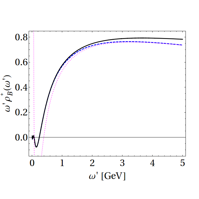
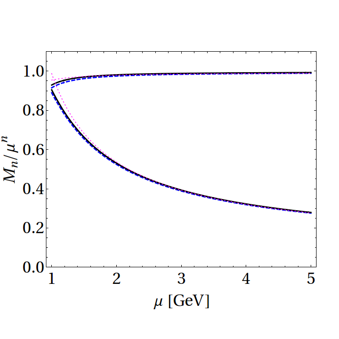
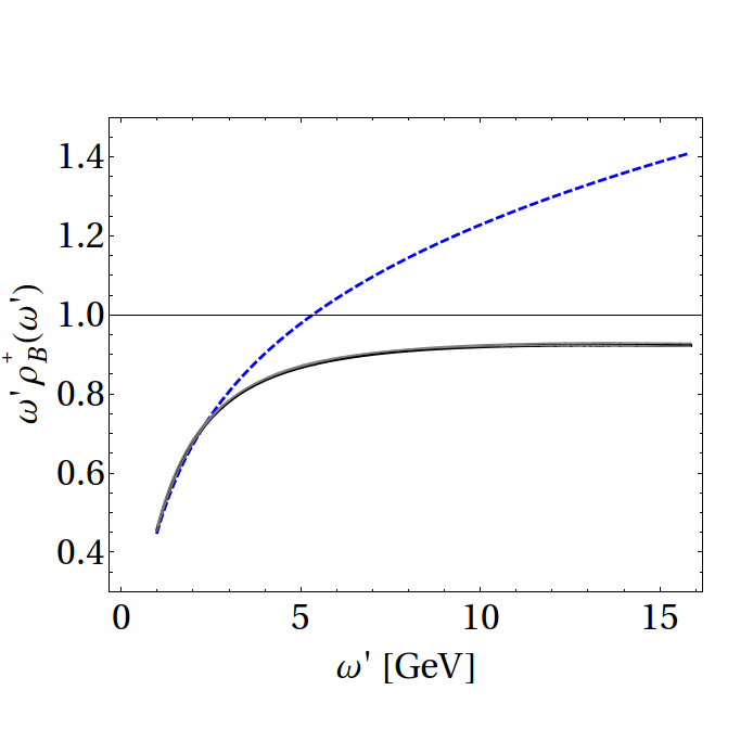
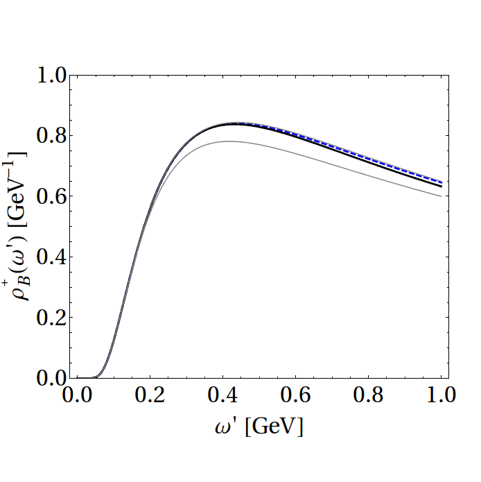
which is valid for . (Notice that the implicit -dependence from the auxiliary scale cancels between the two factors in (33) up to higher-order corrections which will be numerically checked by varying the parameter .) The RG-improved form (33) is compared to the result from fixed-order perturbation theory (FOPT) in (25) in Fig. 1. As we discuss below, our new idea of local RG improvement is essential for the understanding of the asymptotic behaviour of for . However, this resummation will only slightly modify the positive moments compared to the FOPT expressions in (16), as long as and are sufficiently large and of similar size. This is illustrated in Fig. 2.
For a given (high) scale and large values of , the dual function is thus completely determined perturbatively — independent of any hadronic model — with
| (34) |
IV Construction of
Our aim is now to find a systematic parametrization for the dual function which interpolates between some low-energy model (valid at small renormalization scales and small values of ) and the perturbative behaviour in (34), with the following features:
-
•
Explicit implementation of the RG evolution as discussed above.
-
•
Correct behaviour at large values of , such that the constraints on positive moments of ) in HQET, as discussed above, are fulfilled.
Starting from a model function , which is supposed to have a Taylor expansion in at large values of and to give a good description of the low- region, we then propose the following ansatz
| (35) | |||
| (36) | |||
| (37) |
In the first line we start with a given model for the dual function and subtract a number of terms, with representing a set of appropriate functions which reduce to a power-law behaviour for large values of , and vanish quickly at small . The term in square brackets then reduces to for small values of but now decreases as at large values of . The evolution factor in front is chosen to refer to a hadronic reference scale assigned to the input model 222If the hadronic model under consideration gives an explicit reference to the renormalization scale , one would have to replace in .. The term in the second line uses the same set of basis functions to reproduce the RG-improved perturbative result in (33).
In the following analysis, we take the first two coefficients in that sum into account (). The coefficients can then be matched by expanding the corresponding perturbative or model functions for large values of , which will be done below. For the set of functions we choose
| (39) |
so that the modifications from the perturbative matching are exponentially suppressed at small values of , where the original model is supposed to give a reasonable functional description. The auxiliary parameter sets the scale where the transition between the perturbative and non-perturbative regime occurs.
IV.1 Models
The coefficients can easily be extracted by comparing the Taylor expansion in . For instance, for the exponential model
| (40) |
one obtains
| (41) |
and for the free parton model Kawamura:2001jm , as discussed in Bell:2013tfa ,
| (42) |
one gets
| (43) |
As a third illustrative model, we consider the tree-level estimate of a QCD sum-rule analysis in Braun:2003wx where which corresponds to
| (44) |
and
| (45) |
IV.2 Matching with OPE
The ansatz (LABEL:ansatz) reduces straight-forwardly to an expression in FOPT by setting . The matching coefficients are then easily obtained by equating the resulting large- expansion with (26). For the first two coefficients, we obtain
| (46) | ||||
| (47) | ||||
| (48) |
Notice that, at this stage, the parameter is arbitrary. However, as we will see in the numerical analysis, the dependence of the on the value of is not very pronounced. For concreteness, we will use a default value of .
V Logarithmic Moments
The logarithmic moments of the dual function can be defined as
| (49) |
As emphasized in Bell:2013tfa the first three logarithmic moments () of are identical to those of . They represent the hadronic input parameters appearing in factorization theorems for exclusive -meson decays to first non-trivial order in the strong coupling constant.
- •
-
•
For the contributions from , substituting ,
(52) we may expand the function in terms of Laguerre polynomials ,
(53) For a given model, the coefficients can be obtained from the orthogonality relation (61). The logarithmic moments simply follow as
(54) (55) (56) etc. (57)
In principle the first few – and hence the first few – can be determined from precision analyses of radiative leptonic -meson decays (see Beneke:2011nf ; Braun:2012kp for recent discussions). On the theory side the task is difficult. When more information on the perturbative analysis of the moments becomes available, it only affects the precision of our knowledge of , but does not spill over into the non-perturbative contribution. It may be interesting to see if non-perturbative methods like sum rules and lattice QCD are able to shed more light on the Laguerre coefficients in , once the dual function is used in lieu of .
V.1 Large-Scale Behaviour
As we have seen, at tree-level in FOPT the dual function behaves as for large values of , see (26). This behaviour is softened by (global) evolution towards higher scales, i.e.
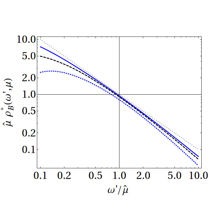
in (10), which induces an additional factor . Therefore it appears as if for sufficiently large values of the -integrals which, for instance, determine the transformation back to -space in (7) or the logarithmic moments in (49), would no longer converge. (In other words it seems as if undergoes a qualitativ change by evolving to sufficiently large scales such that .) The local RG improvement as it is implemented in (33) reveals, however, that the perturbative resummation of logarithms from the region always yields converging results, since at large (but fixed) values of one rather has
and for . Therefore, in that asymptotic region, the function always decreases faster than , which can also be seen from Fig. 3 where we compare the behaviour of at different renormalization scales.
For phenomenological applications in exclusive -meson decays one always has , but we may still formally consider the case for curiosity. From the discussion in the previous paragraph, we conclude that the solution of the RGE for the dual function makes sense for arbitrary values of and (provided they are sufficiently larger than ). In contrast, the derivation of the RGE solutions for the original LCDA in (2) – as discussed in Lee:2005gza ; Kawamura:2001jm – is formally restricted to values . So we repeat for clarity’s sake that the logarithmic moments exist at all scales , and that perceived thresholds are mathematical artifacts.
VI Numerical Examples
VI.1 Preliminaries
Mass-renormalization and :
For the numerical analysis, we take the -quark mass from a determination in a different mass scheme, the shape-function (SF) scheme Bosch:2004bt , which is related to the pole-mass scheme via
| (58) |
with a fixed reference scale . The HFAG 2013 update Amhis:2012bh quotes
for a common value GeV. For the numerical discussion in the pole-mass scheme 333In this work we do not entertain the idea to change the mass scheme in the perturbative matching procedure itself. Although a renormalon-free scheme like the one proposed in Lee:2005gza would improve the perturbative convergence for the regularized moments , we do not expect a significant effect for the logarithmic moments relevant for phenomenological applications since, as we will show below, the contributions from the perturbative regime are subdominant there. , this corresponds to using
Hadronic reference scale:
As our default choice for a hadronic reference scale, we use
The dimensionless parameter in (32) is taken at a default value and varied between and . As already mentioned above, our default choice for the scale-parameter in the functions is set to
Again this value will be varied within a factor of to study the sensitivity
of our parametrization with respect to this parameter.
Running coupling constant:
For we take the 3-loop formula (66) with a fixed number of flavours , and MeV, which corresponds to
We also take into account the 3-loop -function in the evaluation
of the RG function (see appendix).
Model 1:
The parameter
in (40) at GeV is set to MeV,
where we have used the value advocated in Lee:2005gza .
Model 2:
The free parton model does not involve additional
hadronic parameters, except for the HQET parameter
, together with the low-energy
reference scale , which have already been fixed above.
Model 3:
The tree-level sum rule estimate in Braun:2003wx
contains a parameter GeV at GeV.
VI.2 Illustrations
at large values of :
In Fig. 4, we present the result for the product
at large values for two
choices of renormalization scale, GeV and GeV.
We observe
that the inclusion of the radiative corrections
shows a significant effect compared to the original (tree-level) functions
, while the differences among
the different models is irrelevant at large values of .
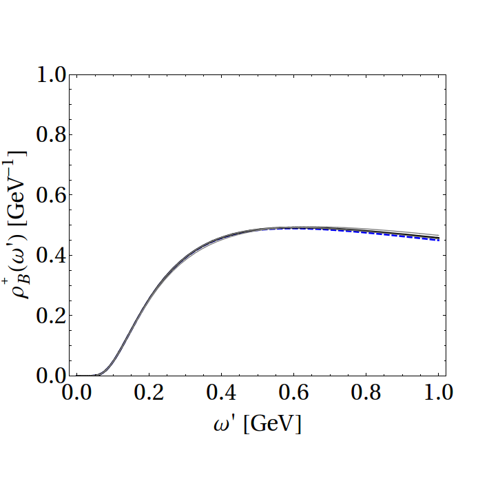
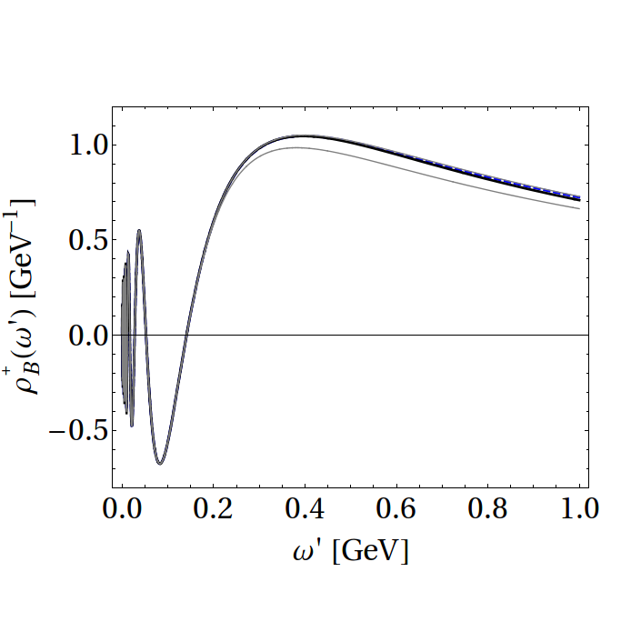
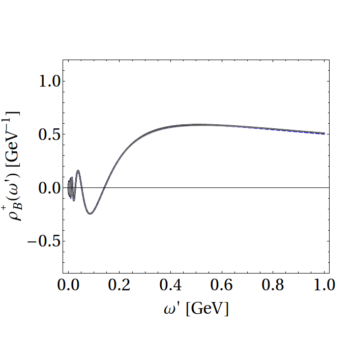
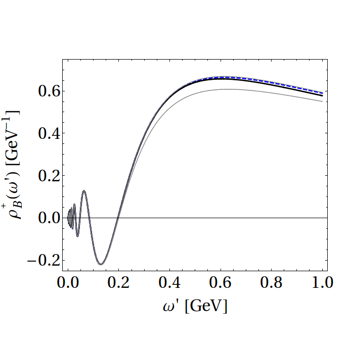
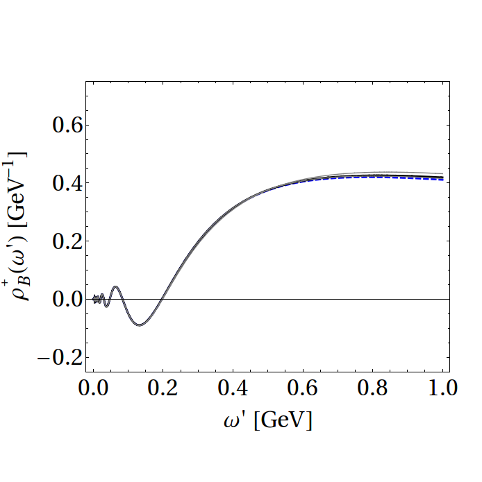
at small values of :
In Fig. 5, we present the results for
at small values for two choices of renormalization scale,
and GeV. We observe that for our default value of the parameter
the original model is reproduced extremely well, and the variation of this parameter
has only a minor effect at intermediate values of .
The LCDA :
From the QCD-improved dual function in (LABEL:ansatz) for a given
input model, we can easily compute the corresponding LCDA
via (7) by numerical integration.
We have compared the
original (tree-level) models of and their QCD-improved versions
for the 3 benchmark models. For all three models we recovered the feature
of a (negative) “radiative tail”
at large values of Lee:2005gza , while the
behaviour at small values of is practically unaffected.
Regularized moments of :
In Table 1 we list the first two (regularized) moments
and as obtained from different models and different renormalization scales,
and compare them to the perturbative result obtained from the local RG-improved
formula (33). Here, the value for the UV cutoff is chosen slightly
larger than the renormalization scale, ,
in order to assure that the result is sufficiently dominated by the radiative
tail in the corresponding LCDA .
We observe that the zeroth moment is reproduced rather
accurately by the different models; the first moments differ more, around 10% at GeV. These
differences are easily explained by the fact that those higher-order terms
in which are not fixed by the matching procedure are of the order
relative to .
| model-1 | model-2 | model-3 | pert. (RG) | ||
|---|---|---|---|---|---|
| 3 GeV | 0.996 | 0.995 | 0.998 | 0.988 | |
| 6 GeV | 1.032 | 1.024 | 1.036 | 0.993 | |
| 10 GeV | 1.011 | 1.004 | 1.014 | 0.995 | |
| 3 GeV | 0.454 | 0.383 | 0.494 | 0.393 | |
| 6 GeV | 0.329 | 0.287 | 0.351 | 0.250 | |
| 10 GeV | 0.207 | 0.183 | 0.219 | 0.188 |
Logarithmic Moments:
| total | from | from | |
|---|---|---|---|
| (model 1) | 1.67 | 1.58 | 0.086 |
| (model 2) | 1.65 | 1.57 | 0.086 |
| (model 3) | 1.21 | 1.12 | 0.086 |
| (model 1) | -3.85 | -3.93 | 0.074 |
| (model 2) | -3.46 | -3.54 | 0.074 |
| (model 3) | -2.19 | -2.27 | 0.074 |
| (model 1) | 11.6 | 11.4 | 0.121 |
| (model 2) | 9.03 | 8.91 | 0.121 |
| (model 3) | 5.44 | 5.32 | 0.121 |
total (RG)
FOPT
input (tree)
(model 1)
2.19
2.12
2.28
(model 2)
2.05
1.98
2.15
(model 3)
1.40
1.34
1.50
(model 1)
-3.31
-3.45
-3.20
(model 2)
-2.41
-2.56
-2.31
(model 3)
-1.31
-1.46
-1.21
(model 1)
7.88
7.19
8.25
(model 2)
4.25
3.56
4.62
(model 3)
2.48
1.80
2.85
In Table 2, we compare the numerical results for
the first three logarithmic moments following from the
three different benchmark models.
In the upper part, we consider an intermediate scale
GeV and separate the contributions to the integral from regions where is smaller or larger than .
We observe that the former – by construction – very much depend on the specific hadronic input model.
The contributions to the moments
from large values, , on the other hand,
are completely determined by perturbative matching and RG evolution
and therefore independent of the
hadronic input model, in line with the discussion around
(34).
In the lower half of the table, we illustrate the effects of the perturbative constraints
by comparing the moments originating from the hadronic input function with its modifications
from FOPT alone and its (locally) RG-improved version, at the hadronic input scale GeV.
Again, we observe that the logarithmic moments before and after the perturbative improvement
are highly correlated and do not differ very much.
VII Summary
The dual function of the heavy B-meson, which plays a similar role to the familiar set of Gegenbauer coefficients for light-meson LCDAs, has been the subject of this paper. To recapitulate and summarize we have highlighted that the transformation between the LCDAs in momentum space, , and dual momentum space, , consists of eigenfunctions of the RG evolution kernel for . The dual function renormalizes multiplicatively, unlike the LCDA , which in particular implies that the non-perturbative low- region does not mix with the perturbative domain, .
We have demonstrated that the dual function in the perturbative domain is calculable from the OPE results of a finite-moment analysis of Lee:2005gza , and determined its values in the region . By resumming perturbative logarithms we have shown that vanishes faster than for , such that its first inverse moment, , converges for at any perturbative scale . This result distinguishes the analysis of and related quantities in dual momentum space from the corresponding one using the standard LCDA , which appears to suffer from artificial thresholds in its RG evolution when the RG function assumes positive integer values.
The low- regime is not accessible via perturbation theory. It must be determined by other means, but can be modelled in the meantime. We have developed a method of combining a model ansatz in the non-perturbative regime with the perturbative results that respects the moment constraints and smoothly connects both domains. This was achieved by correcting the first few terms in the large- behaviour of the model, which is shown in Eq. (LABEL:ansatz). The keen-eyed reader might inquire whether taking ever more terms into account in this manner will ultimately determine the dual function and thus render the modelled part superfluous. We found only poor or no convergence with such an approach, depending on the choice of basis functions , which points towards an unrelatedness between and other HQET parameters like within perturbative methods.
We have illustrated our results using three different models, and also performed a numerical analysis for the phenomenologically relevant logarithmic moments . Following the gist of our discussion thus far, we split between the regions and . While the contributions are model-independent (and small), the hadronic model dominates the moments. In principle the can be determined from precision analyses of radiative leptonic -meson decays, but this only determines the first few terms in an expansion of the dual function in terms of Laguerre polynomials in the variable for .
The perturbative analysis of the -meson LCDA is restricted to 1-loop accuracy so far. From the theoretical perspective, it would be interesting to see to what extent the picture that emerged from our analyses continues to be valid when implementing 2-loop corrections to the evolution kernel and the perturbative moment constraints, together with higher power corrections in HQET.
Acknowledgements.
TF and BOL acknowledge support by the Deutsche Forschungsgemeinschaft (DFG) within the Research Unit FOR 1873 (Quark Flavour Physics and Effective Field Theories). YMW is supported by the DFG-Sonderforschungsbereich/Transregio 9 “Computergestützte Theoretische Teilchenphysik”. We are particularly grateful to Guido Bell who continually accompanied the project and contributed many valuable discussions and comments and critical reading of the manuscript. TF also would like to thank Thomas Mannel for helpful discussions.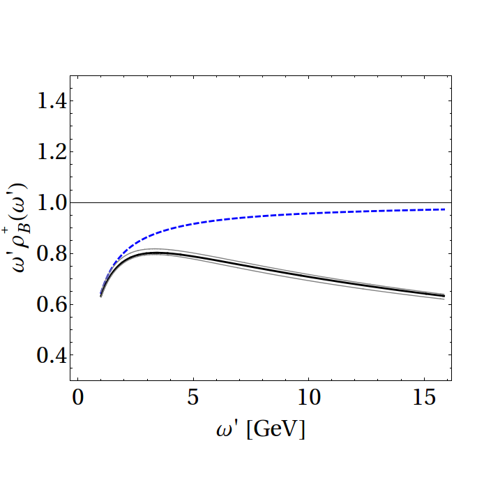
Appendix A Some Properties of Special Functions
We use the completeness relation for Bessel functions in the form
| (59) |
Among others, this allows to revert the relation between the regularized moments and the dual function for large values of
| (60) |
The Laguerre polynomials satisfy the orthogonality relation
| (61) |
The explicit expressions for read
| (62) |
Appendix B Explicit Form of RG Functions
The expansions of the QCD -function and the anomalous dimensions in the LN kernel are defined as
| (63) |
with
| (64) | |||
| (65) |
With this we express the 3-loop running coupling constant as
| (66) |
For the considered range of RG scales, we take with MeV.
The coefficients in the perturbative expansion of the cusp anomalous dimension,
| (68) |
read Korchemsky:1987wg ; Korchemskaya:1992je ; Moch:2004pa
| (69) | |||
| (70) |
The RG elements have been defined in (10) as
| (72) |
with the RG functions and defined as (see e.g. Neubert:2004dd )
| (73) |
In order to make the composition rule (11) manifest, it is convenient to introduce a reference scale, , which in the numerical analysis we identify with the hadronic input scale . To this end, we rewrite the function as
| (74) | ||||
| (75) |
With this, the RG elements read
| (76) |
and, by definition,
| (77) |
which implies the composition rule for . Explicit expansions for the RG functions can now be obtained by inserting the perturbative expressions for the -function and anomalous dimension. Using the abbreviations
| (78) |
we find to 3-loop accuracy,
| (79) | ||||
| (80) |
Similarly, for the function one gets
| (81) | ||||
| (82) |
where we neglected terms of order ,
as the 2-loop result for the anomalous-dimension coefficient ,
which will enter at that order,
is currently unknown. Notice that the so constructed expansions of and ,
and thus the expansion of ,
respect the composition rule (which would not have been the case if one
had expanded the function directly).
References
- (1) G. Bell, Th. Feldmann, Y.-M. Wang and M. W. Y. Yip, JHEP 1311 (2013) 191 [arXiv:1308.6114 [hep-ph], arXiv:1308.6114].
- (2) B. O. Lange, M. Neubert, Phys. Rev. Lett. 91 (2003) 102001 [hep-ph/0303082].
- (3) S. J. Lee, M. Neubert, Phys. Rev. D 72 (2005) 094028 [hep-ph/0509350].
- (4) M. Beneke, G. Buchalla, M. Neubert and C. T. Sachrajda, Phys. Rev. Lett. 83 (1999) 1914 [hep-ph/9905312].
- (5) Z. Ligeti, I. W. Stewart and F. J. Tackmann, Phys. Rev. D 78 (2008) 114014 [arXiv:0807.1926 [hep-ph]].
- (6) P. Ball and A. N. Talbot, JHEP 0506 (2005) 063 [hep-ph/0502115].
- (7) A. G. Grozin and M. Neubert, Phys. Rev. D 55 (1997) 272 [arXiv:hep-ph/9607366].
- (8) G. Bell and T. Feldmann, JHEP 0804 (2008) 061 [arXiv:0802.2221 [hep-ph]].
- (9) M. Knodlseder and N. Offen, JHEP 1110 (2011) 069 [arXiv:1105.4569 [hep-ph]].
- (10) S. Descotes-Genon and N. Offen, JHEP 0905 (2009) 091 [arXiv:0903.0790 [hep-ph]].
- (11) A. V. Efremov and A. V. Radyushkin, Phys. Lett. B 94 (1980) 245.
- (12) G. P. Lepage and S. J. Brodsky, Phys. Lett. B 87 (1979) 359; Phys. Rev. D 22 (1980) 2157.
- (13) H. Kawamura, J. Kodaira, C. -F. Qiao, K. Tanaka, Phys. Lett. B 523 (2001) 111 [Erratum-ibid. B 536 (2002) 344] [hep-ph/0109181]; H. Kawamura and K. Tanaka, Phys. Lett. B 673 (2009) 201 [arXiv:0810.5628 [hep-ph]].
- (14) V. M. Braun, D. Y. Ivanov and G. P. Korchemsky, Phys. Rev. D 69 (2004) 034014 [arXiv:hep-ph/0309330].
- (15) M. Beneke and J. Rohrwild, Eur. Phys. J. C 71 (2011) 1818 [arXiv:1110.3228 [hep-ph]].
- (16) V. M. Braun and A. Khodjamirian, Phys. Lett. B 718 (2013) 1014 [arXiv:1210.4453 [hep-ph]].
- (17) S. W. Bosch, B. O. Lange, M. Neubert and G. Paz, Phys. Rev. Lett. 93 (2004) 221801 [hep-ph/0403223].
- (18) Y. Amhis et al. [Heavy Flavor Averaging Group Collaboration], arXiv:1207.1158 [hep-ex].
- (19) G. P. Korchemsky and A. V. Radyushkin, Nucl. Phys. B 283 (1987) 342.
- (20) I. A. Korchemskaya and G. P. Korchemsky, Phys. Lett. B 287 (1992) 169.
- (21) S. Moch, J. A. M. Vermaseren and A. Vogt, Nucl. Phys. B 688 (2004) 101 [hep-ph/0403192].
- (22) M. Neubert, Eur. Phys. J. C 40 (2005) 165 [hep-ph/0408179].
- (23) V. M. Braun and A. N. Manashov, arXiv:1402.5822 [hep-ph].