Understanding Machine-learned Density Functionals
Abstract
Kernel ridge regression is used to approximate the kinetic energy of non-interacting fermions in a one-dimensional box as a functional of their density. The properties of different kernels and methods of cross-validation are explored, and highly accurate energies are achieved. Accurate constrained optimal densities are found via a modified Euler-Lagrange constrained minimization of the total energy. A projected gradient descent algorithm is derived using local principal component analysis. Additionally, a sparse grid representation of the density can be used without degrading the performance of the methods. The implications for machine-learned density functional approximations are discussed.
pacs:
31.15.E-, 31.15.X-, 02.60.Gf, 89.20.FfI Introduction
Since the early days of quantum mechanics, it has been known that sufficiently accurate solutions of Schrödinger’s equation for electrons and nuclei yield good predictions of the properties of solids and molecules Dirac (1929). But the Coulomb repulsion between electrons causes the computational cost of solving the Schrödinger equation to grow rapidly with the number of electrons, Kohn (1999). However, as Hohenberg and Kohn proved in 1964 Hohenberg and Kohn (1964), the one-electron density may be used as the basic variable of quantum mechanics instead of the wavefunction, greatly reducing the complexity of the computational problem. This is called density functional theory (DFT) Dreizler and Gross (1990). In principle, the mapping of the Schrödinger equation to one with the electron density is exact, but in practice, both the kinetic energy and the energy of the interaction between electrons must be approximated. In the original Thomas-Fermi theory Thomas (1927); Fermi (1928), a local density functional approximation to the kinetic energy is used. However, Thomas-Fermi theory proved unsuitable for chemical and solid-state applications as it does not bind matter Teller (1962). Shortly after the Hohenberg-Kohn theorems, Kohn and Sham (KS) Kohn and Sham (1965) found a middle ground by mapping the many-body system onto a fictitious system of non-interacting electrons which reproduce the exact electron density. The main reason KS DFT became successful is because the kinetic energy of these non-interacting electrons is an excellent approximation to the many-body kinetic energy. Simple approximations to the interaction energy produce much greater accuracy and reliability compared with the standard orbital-free DFT schemes built on Thomas-Fermi theory. However, the accuracy of the results are still sensitive to the approximation of the exchange-correlation (XC) functional. In the past four decades, there has been extensive research into improving density functional XC approximations. Development of both empirical and non-empirical functionals require great intuition built on years of experience, as well as painstaking trial and error Becke (1988); Lee et al. (1988); Perdew et al. (1996).
Despite the great success KS DFT has enjoyed, the computational cost scales as , which is much worse than the linear scaling of orbital-free DFT Karasiev and Trickey (2012). Thus, there continues to be strong interest in improving upon existing orbital-free approximations to the kinetic energy Karasiev et al. (2009a); Karasiev and Trickey (2012); Tran and Wesolowski (2002a). A sufficiently accurate approximation to , the kinetic energy of KS electrons as a functional of the ground-state density would enable highly accurate orbital-free DFT calculations with the same accuracy as KS DFT at a fraction of the computational cost. For example, benchmark orbital-free DFT calculations are capable of treating millions of atoms in metals Hung and Carter (2009) or proteins in solvent Hodak et al. (2008). Note that accuracy in beyond that of current XC approximations would be unnecessary, since all standard orbital-free DFT schemes utilize the KS decomposition of the energy, so that standard XC approximations developed for KS DFT can be utilized. However, since is typically comparable to the total energy of the system Dreizler and Gross (1990), an unavoidable problem is that a useful kinetic energy (KE) functional calls for much stricter relative accuracy than XC functionals. Additionally, accurate functional derivatives are required because one finds the ground state density by solving an Euler equation with the approximate kinetic energy functional. Continued efforts have been made in this research direction, with some notable progress Weizsäcker (1935); Wang and Carter (2000); Karasiev et al. (to appear, 2009b, 2013); Tran and Wesolowski (2002b); Chacón et al. (1985); García-González et al. (1996, 1998); Wang and Teter (1992); Wang et al. (1999); Xia et al. (2012). For a review of state-of-the-art orbital-free DFT functionals, we refer the reader to Ref. Karasiev and Trickey (2012).
In DFT, functionals typically fall into two categories. Non-empirical functionals derived from first principles tend to work well across a broad range of systems, and may exhibit systemic errors in treating certain types of interactions. Semi-empirical functionals introduce parameters that are fitted to standard data sets, and are typically more accurate with less systematic errors.
Recently, some of us applied machine learning (ML) in a completely new approach to approximating density functionals Snyder et al. (2012, 2013). In a proof of principle, kernel ridge regression was used to approximate the kinetic energy of non-interacting fermions confined to a 1d box as a functional of the electron density Snyder et al. (2012). In that work, a modified orbital-free DFT scheme was able to produce highly accurate self-consistent densities and energies that were systematically improvable with additional training data. ML algorithms are capable of learning high-dimensional patterns by non-linear interpolation between given data. These powerful methods have proved to be very successful in many applications Müller et al. (2001), including medical diagnoses Kononenko (2001), stock market predictions Huang et al. (2005), automated text categorization Sebastiani (2002), and others. Recently, ML has been applied to quantum chemistry, including fast and accurate modeling of molecular atomization energies Rupp et al. (2012); Hansen et al. (2013); Montavon et al. (2013a), optimizing transition state theory dividing surfaces Pozun et al. (2012), and calculating bulk crystal properties at high temperatures Bartók et al. (2010).
This new approach to density functional approximation suffers none of the typical challenges found in traditional approximations, but presents many new ones. First and foremost, ML is data-driven: reference calculations are needed to build a model for the KE functional. Since every iteration in a KS DFT calculation provides an electron density and its exact non-interacting KE, reference data is relatively easy to obtain. Additionally, the ML approximation (MLA) to the KE may have thousands or millions of parameters and satisfy none of the standard exact conditions in DFT, such as positivity, scaling, and exactness for a uniform electron gas. On the other hand, the form of the MLA is completely general and thus directly approximates the functional itself, suffering none of the typical issues plagued by standard functionals starting from a local approximation. For example, some of us recently showed that an MLA for the KE has no problem accurately dissociating soft-Coulomb diatomics in 1d—a huge challenge for standard approximations Snyder et al. (2013). However, kernel ridge regression is strictly a method of interpolation. An MLA can only be used on systems it was designed for.
In this paper, we explore the properties of the MLA derived in Ref. Snyder et al. (2012) in greater detail. In particular, we investigate the use of various kernels and their properties and the efficiency of various cross validation methods. We discuss the issue of functional derivatives of the MLA in greater detail, and explain how a modified constraint to the standard Euler equation enables highly accurate self-consistent densities, or constrained optimal densities, to be found. Additionally, a projected gradient descent algorithm is derived using local principal component analysis in order to solve the modified Euler equation. Finally, we explore the use of a sparse grid representation of the electron density and its effects on the method.
II Theory and Background
Throughout this work, we consider only non-interacting same-spin fermions in one-dimension. Thus, all electron densities are fully spin-polarized. Atomic units are used in symbolic equations, but energies are usually presented in .
II.1 Model system
Consider non-interacting same-spin fermions subject to a smooth external potential in one-dimension, with hard walls at and . We restrict this study to a simple class of potentials, namely a sum of 3 Gaussian dips with varying heights, widths and centers:
| (1) |
for , and elsewhere. The Hamiltonian for this system is simply , where and . We solve the Schrödinger equation
| (2) |
for the eigenvalues and orbitals . As our fermions are same-spin, each orbital is singly-occupied. Thus, the electron density is given by
| (3) |
and the kinetic energy is
| (4) |
A dataset is created by randomly sampling , to generate 2000 different potentials. For each potential, the system is occupied with up to 4 fermions, and the exact densities and kinetic energies are computed. Numerically, the Schrödinger equation is solved by discretizing the density on a grid:
| (5) |
and is the grid spacing. Numerov’s method Hairer et al. (1993) together with a shooting method is used to solve for the eigenvalues and eigenfunctions of Eq. (2). For , the error in our reference kinetic energies is less than . Fig. 1 gives a few sample densities and their corresponding potentials.
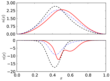
The data used here is identical to that of Ref. Snyder et al. (2012). The exact values of the parameters used in each sample is given in the supplementary information of Ref. Snyder et al. (2012). Of the 2000 samples generated, the first half is reserved for training while the second half is reserved for testing (which we refer to as the test set).
II.2 Orbital-free DFT
In orbital-free DFT, is approximated as a functional of . For our model system with non-interacting fermions, the total energy is given as
| (6) |
for a given potential . The potential is known exactly as a functional of :
| (7) |
Via the variational principle, the ground-state density is found by the Euler-Lagrange constrained search
| (8) |
where the chemical potential is adjusted to produce the required particle number . This becomes simply
| (9) |
The density that satisfies this equation, minimizing with the normalization constraint, is found self consistently.
Given the exact functional , solving Eq. (9) will yield the exact ground-state density of the system. But in practice, must be approximated. Let be such an approximation, be the exact density, and be the self-consistent density found with . There are two measures of the error of such an approximate Kim et al. (2013). The first is to compute the functional-driven error , which is simply the error in the KE evaluated on the exact density. The second (and much more difficult) test is to insert into Eq. (9), solve for the approximate density , and compute its error relative to the KE of the exact density . Then the density-driven error is defined as Kim et al. (2013). This is the additional error incurred by the approximate density. In practice, a functional which only satisfies the first test is not much use, as the ground-state density itself must also be obtained from this approximation. In orbital-free DFT, self-consistent results can be much worse than energies of KS densities, as inaccuracies in the functional derivative can cause large errors in the corresponding density. In the case of the KE functional for real systems, functional derivatives of traditional approximations can have singularities at the nuclei, making all-electron calculations very difficult, if not impossible, to converge Karasiev and Trickey (2012). Many of these problems can be avoided through use of pseudopotentials Karasiev and Trickey (2012); Xia et al. (2012), but in general the solution for Eq. (9) is nontrivial.
As mentioned above, the simplest density functional approximation to is the local approximation Dreizler and Gross (1990), which for spin-polarized densities in 1d is
| (10) |
For , the exact KE has the von Weizsäcker Weizsäcker (1935) form:
| (11) |
As was shown in Ref. Snyder et al. (2012), the local approximation does poorly. The mean absolute error (MAE) on the test set is 217 kcal/mol, and self-consistent results are even worse at 1903 kcal/mol. A standard extension of the local approximation to a semi-local form is to add a fraction of to , forming a modified gradient expansion approximation. It was shown in Ref. Snyder et al. (2012) that this did little to improve upon the local approximation.
II.3 Data topology and representation
Typically in ML, the data has a finite representation. For example, in Ref. Rupp et al. (2012), molecular structures are represented by a Coulomb matrix and the model predicts atomization energies. In contrast, the electronic density is a continuous function restricted to the domain Lieb (2002)
| (12) |
where is a Sobolev space111 A Sobolev space is a vector space of functions with a norm that is a combination of -norms of the function itself and its derivatives up to a given order . It is conventional to write as . means that and its first order derivative are in .. Although is infinite dimensional, in practice is expanded in a finite basis (with basis functions). In this work, we use a real space grid to represent the density, since our reference calculations are done using the same grid. We use the inner product and norm between densities
| (13) |
(In actual calculations, all densities are represented on a finite basis, and thus will have have a finite -norm). Since the ML algorithm is expressed in terms of this inner product, the results are independent of the specific representation used as long as the basis is converged.
Even with a truncated basis, is still high-dimensional and applying ML to learn the KE of all densities in would not be feasible. Fortunately, we are only interested in a subspace of related to a specific class of potentials (e.g. Gaussian dips), which greatly reduces the variety of possible densities. In general, let the potential be parametrized by the parameters . We define the density manifold as the set of all densities that come from these potentials with a given particle number . In general, is a -dimensional manifold. The training densities, for , are sampled from . In the present work, the external potential has 9 parameters, and thus is at most 9.
II.4 The kernel trick and feature space
In finding the structure of low-dimensional data, it is often sufficient to optimize parametrized non-linear forms (e.g., using a polynomial to fit a sinusoid). For high-dimensional, nonlinear data this becomes increasingly difficult. In kernel-based machine learning, the approach is to transform the data itself non-linearly to a high-dimensional space known as feature space, such that the data becomes linear Vapnik (1995); Scholkopf et al. (1999); Müller et al. (2001); Montavon et al. (2013b); Schölkopf and Smola (2002).

Fig. 2 illustrates data points that lie on a circle in the Cartesian plane. As shown, the data becomes linear on transformation to polar coordinates, and linear regression can subsequently be used to fit the data. Transforming back to Cartesian coordinates recovers the non-linearity. Let the data points belong to a vector space , also called input space, and let be the map to feature space . Assuming we wish to apply a linear method such as regression in feature space , we note that regression can be expressed solely in terms of the inner product between feature vectors and , where . We define the kernel such that
| (14) |
The kernel can generally be thought of a measure of similarity between data, but must satisfy Mercer’s condition:
| (15) |
for all satisfying . Mercer’s theorem Mercer (1909) guarantees the existence of a feature space , which is a reproducing kernel Hilbert space Aronszajn (1950). Since the linear algorithm in may be expressed in terms of the kernel in Eq. (14), need never be explicitly computed. This procedure is known as the kernel trick, and enables easy nonlinearization of all linear scalar product-based methods that can be expressed via an inner product Schölkopf et al. (1998).
II.5 Kernel ridge regression
Kernel ridge regression is a nonlinear version of regression with a regularization term to prevent overfitting Hastie et al. (2009). Our MLA for the KE has the form
| (16) |
where is the number of training densities, are weights to be determined, are training densities and is the kernel. The weights are found by minimizing the quadratic cost plus regularization
| (17) |
where , is the kernel matrix, , and is called the regularization strength. The second term penalizes weights with large magnitudes in order to prevent overfitting.222 The regularization term accounts for the possibility of noisy data (e.g. experimental data), and imposes certain smoothness conditions on the model (see Smola et al. (1998)). Our reference data is deterministic and thus noise-free in this sense, but, because the precision of our calculations is limited, we may consider the numerical uncertainty to be noise. By setting the gradient of Eq.17 to zero, minimizing gives
| (18) |
where is the identity matrix and . The hyperparameters, which include the regularization strength and the parameters of the kernel such as the length scale , are found via cross validation (see Hansen et al. (2013) and Sect. III).
The choice of the kernel will depend on the given data. Some kernels are designed to be generally robust and applicable (e.g., the Gaussian kernel), while others are designed for a specific type of data (see e.g. Rupp et al. (2007); Zien et al. (2000); Müller et al. (2001)). A good choice of kernel can reflect the characteristics of the data (see Braun et al. (2008)). In Ref. Snyder et al. (2012), we chose the Gaussian kernel
| (19) |
where is the length scale. Since the density is represented on a uniform grid, the -norm can be approximated by333 Note that, in Ref. Snyder et al. (2012), the same representation for the density was used, but the density were treated as vectors, so the standard Euclidean distance was used in the kernel. This is equivalent to the formulation here, except our notation is more general now (e.g. Simpson’s rule could be used to approximation the -norm instead of a Riemann sum), and the length scale in Gaussian kernel here is related to the scale of the kernel in Ref. Snyder et al. (2012) by a factor of .
| (20) |
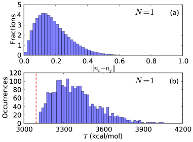
where is given by the grid defined in Eq. (5). This approximation becomes exact as . Fig. 3 shows the range and distribution of Euclidean distances between all pairs of densities and KE of all densities in the dataset with .


Ordinary linear regression models frequently employ a bias term to account for the fact that the data might lie away from the origin. Without this term, the regression line is forced to go through the origin, causing a systematic error if the data does not. The bias term can be implemented directly, or by centering the samples such that the mean is zero. Fig. 4 illustrates the transformation to feature space for an example 1d data set and linear regression in feature space. If the data is centered in feature space, the bias term is unnecessary. Here, we center the densities in features space such that . We define the centered map to feature space . Then the centered kernel is Schölkopf et al. (1998)
| (21) | |||||
For simplicity, all equations given in this work assume that the data is centered (i.e. ). In fact, kernels such as the Gaussian kernel Eq.(19) whose induced reproducing kernel Hilbert space on a bounded domain is dense in the space of continuous functions on this domain do not require centering Poggio et al. (2001).
III Model selection
III.1 Kernels
Model selection refers to the process of selecting a kernel and the corresponding hyperparameters. In kernel ridge regression, this includes the regularization strength and the kernel parameters (e.g. in the Gaussian kernel, the length scale ). Table 1 lists some standard kernels.
| Kernel | |
|---|---|
| Gaussian | |
| Cauchy | |
| Laplacian | |
| Wave | |
| Power | |
| Linear |
Radial basis function (RBF) kernels, which include the Gaussian, Cauchy, and Laplacian kernels, all behave similarly and tend to work for a broad range of problems. Other kernels work well for specific data structures Rupp et al. (2007); Müller et al. (2001); Zien et al. (2000) and regularization properties Schölkopf et al. (1998).
Fig. 5 shows the contours of the functional-driven MAE over the test set as a function of the regularization strength and the kernel parameter . We see that the qualitative behavior is similar for the Gaussian, Cauchy and Laplacian kernels. In the left region (where the contour lines are vertical), the length scale is much smaller than the distance between neighboring training densities. Thus the RBF-type kernel functions centered at each training density have minimal overlap, yielding a poor approximation to the KE functional. The kernel matrix becomes nearly unity, and the regularization has negligible effect. On the right side of the contour plot, the length scale is comparable to the global scale of the data. In these regions, the kernel functions are slowly varying and do not have enough flexibility to fit the nonlinearity in the data. The region with minimum MAE lies in the middle. The Gaussian and Cauchy kernels both give the same performance, with errors less than 1 kcal/mol in the middle region (enclosed by the dashed line), while the Laplacian kernel behaves poorly in comparison. This is likely due to the cusp in the form of the kernel, which cannot fit the smooth KE functional.
III.2 Optimization of hyperparameters
After picking a kernel family, the values of the hyperparameters must be chosen. Ideally, we select the hyperparameters such that the generalization error, which is the error not only on our training set but also on all future data, is minimal. The out-of-sample error must be estimated without looking at the test set (the test set is never touched during model selection, so that it can give a true test of the final performance of the model) Hansen et al. (2013); Müller et al. (2001). This procedure, known as cross-validation, is essential for model selection in preventing overoptimistic performance estimates (overfitting).
Various schemes for cross validation exist Hansen et al. (2013); Müller et al. (2001); Amari et al. (1997), but all obey a basic principle: the available data is subdivided into three parts: the training, validation and the test sets. The ML model is built from the training set and the hyperparameters are optimized by minimizing the error on the validation set (Fig. 6). The test set is never touched until the weights and hyperparameters have been determined. Then and only then, the generalization ability of the model can be assessed with the test data (Müller et al. (2001); Hansen et al. (2013), see also Lemm et al. (2011)).
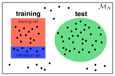
Typically, the data is shuffled to ensure its random distribution between training and validation division. This can be repeated with different subdivisions. A few schemes, which will be analyzed for our kinetic energy functional estimation problem, are described below. For each scheme, a test set of 1000 samples is used to estimate the generalization error after the ML model is selected.
- Simple cross validation
-
The training data ( samples) is randomly divided into a training set of and a validation set of . The hyperparameters are optimized by minimizing the MAE on the validation set.
- -fold cross validation
-
- Step 1
-
The training data is randomly divided into bins.
- Step 2
-
The th bin is used as the validation set and the remaining bins as training set. The model is built on the training set and the hyperparameters are selected by minimizing the MAE on the validation set.
- Step 3
-
Repeat step 2 times such that all bins have been used as validation sets. We will then have models in total and the final hyperparameters are selected as the median over all models.
Because the mean cross validation error still depends on the initial random partitioning of data in cross validation, we repeat the procedure with different subdivisions Müller et al. (2001).
- Leave-one-out
-
Leave-one-out (LOO) is a special case of -fold cross validation, when . Thus each bin contains only one sample.
Typically, it is better to leave out as little data as possible to exploit the statistical power in the data. Simple cross validation is computationally expedient, but wasteful since not all training data participates in the optimization. -fold cross validations are used in situations where data is very limited, or expensive to collect. Leave-one-out is often used with limited data and it becomes computationally intensive if is large. -fold cross validation gives a good balance on all counts.
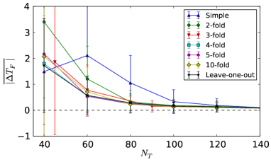
For the Gaussian kernel, Fig. 7 shows the MAE on the test set with the hyperparameters optimized with different cross validation methods. With 120 training densities, all schemes give a similar MAE, despite the large variations in and . This means that multiple models exist that give comparable performance. As expected, the only variations in MAE occur for more limited data.
Fig. 5 shows how -fold cross validation performs in selecting hyperparameters that generalize well to the test set, for a few kernels. The gray dots represent the optimal parameter choice for each repetition, and the black dot is the median over all repetitions. In this case, the global minimum of the MAE lies in a relatively flat basin. Each randomized cross validation lies near the true minimum, indicating the model generalizes well to the test set.
| Kernel | ||||
|---|---|---|---|---|
| Gaussian | 1.6 | 0.13 | 3.4 | |
| Cauchy | 3.5 | 0.13 | 2.9 | |
| Laplacian | 6.4 | 231 | ||
| Linear | - | 53.1 | 380 | |
| Wave | 0.14 | 19.2 | 252 | |
| Power | 1.96 | 3.3 | 104 |
Finally, we use 10-fold cross validation (repeated 40 times) to optimize the hyperparameters. Table 2 shows the optimal hyperparameters and functional driven errors for the kernels listed in Table 1. Some optimum values for the Gaussian kernel are listed in Table 3. Detailed information with optimum values of other kernels are shown in supplementary material.
IV Results and Discussion
In the main work of this paper, we test in greater detail some of the methods that were introduced in Ref. Snyder et al. (2012) using only the Gaussian kernel, as it performs the best.
| Mean | Max | Mean | Max | Mean | Max | ||||
IV.1 Errors on exact densities
In Table 3, we evaluate our MLA, constructed using the first training densities in our data set, on the exact densities of the test set and compute the errors . The Gaussian and Cauchy kernels give the best performance. For the Gaussian kernel with chemical accuracy is achieved (i.e. MAE less than 1 kcal/mol) at . Just as we saw in Ref. Snyder et al. (2012), the performance is systematically improvable with increasing number of training densities. The Laplacian kernel gives a mean absolute error (MAE) of kcal/mol at (still better than LDA), which improves as increases. On the other hand, the performance of the wave kernel does not improve as increases (see supplemental information). This indicates the form of the wave kernel is not flexible enough to fit the form of the KE functional.
IV.2 Sparse grid
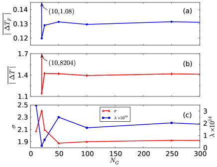
Note that the choice of used in the reference calculations is needed to converge our reference energies and densities, but may be larger then the grid needed to “converge” our ML functional. As the ML model depends only on the inner product between densities, this will typically converge much faster than, e.g. Numerov’s method. To demonstrate this, we define a “sparse” grid, , using every th point in the grid (we only choose such that is divisible by ).
Fig. 8 shows that performance of the model is unaffected until is reduced to about 10 grid points. The model is cross-validated each time, but the hyperparameters change only slightly. Thus, ML can accurately learn the KE functional with a far less complete basis than is required to accurately solve the Schrödinger equation. This is possible because we have restricted the learning problem to a simple type of potential with a limited range of possible densities and energies. The underlying dimensionality of the data is about 9, comparable to the number of parameters that determine the potential. The model needs only enough degrees of freedom in the representation of the density to distinguish between densities, but no more. Thus it is no coincidence that the minimum grid required is comparable to the dimensionality of the data (i.e. the dimensionality of the density manifold ).
However, we also need a sufficiently fine grid to compute the integral in Eq. (7) to the desired accuracy. In the problem shown here, the dimensionality of the data is relatively small, and will increase for larger systems (e.g. real molecules with many degrees of freedom). In general, however, we need to consider both factors in choosing a suitable basis. But, we may be able to use a basis that is more sparse than that of the reference data, which would greatly reduce the computational cost of the method.
IV.3 Challenge of finding density
Thus far, we have focused on the discussion of the performance of the MLA evaluated on exact densities (i.e. the functional-driven errors). However, in order for a functional to be useful, it must also predict the ground-state density. As discussed previously, an accurate functional derivative is necessary in order to solve Eq. (9) and yield an accurate density. The functional derivative of our MLA is given by:
| (22) |
where, for the Gaussian kernel,
| (23) |
In Fig. 10, we plot the functional derivative of our model compared with the exact derivative. The model displays a highly inaccurate functional derivative, with a huge amount of apparent “noise”, as was found in Ref. Snyder et al. (2012).
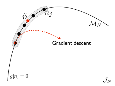
What is the source of this noise? In general, if the underlying dimensionality of the data is much less than the dimensionality of (which in this case is essentially infinite), ML will be unable to capture the functional derivative. The functional derivative contains information on how the KE changes along any direction, but ML cannot learn this because it only has information in directions in which it has data (i.e. along ). Fig. 11 illustrates the problem: standard minimization techniques will rapidly exit the “interpolation” region in which the MLA is expected to be accurate. The MLA is only given information about how the KE changes along the density manifold . In the many dimensions orthogonal to , the MLA produces an inaccurate derivative (each of these dimensions produces a large relative error since no data exists in these directions; the sum over many dimensions creates a large total error in functional derivative). A standard gradient descent will quickly venture off of into regions of where the model is guaranteed to fail. Fig. 9 shows the deviation of self-consistent density if the search is not constrained to .
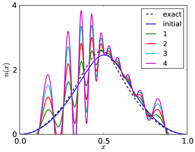
To fix this, we further constrain the minimization in Eq. (9) to stay on . The Euler-Lagrange minimization for the ground-state density can be expressed as
| (24) |
where is any function that is zero on and positive elsewhere. Thus implicitly defines the density manifold . Since any satisfies the normalization condition, the previous constraint is no longer necessary. Because the minimizing density (i.e. the ground-state density) is in and thus satisfies the constraint , Eq. 24 gives the same solution as Eq. 9. Essentially, we have vastly reduced the domain of the search from to . To avoid confusion, we call the minimizing density of this equation the constrained optimal density. It may be solved self-consistently in the same sense of solving the standard Euler equation. However, the which exactly gives the density manifold is unknown. In the next section, we develop an approximation which attempts to reconstruct the density manifold from the training densities.
(a)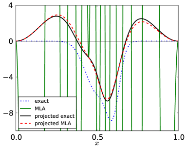 (b)
(b)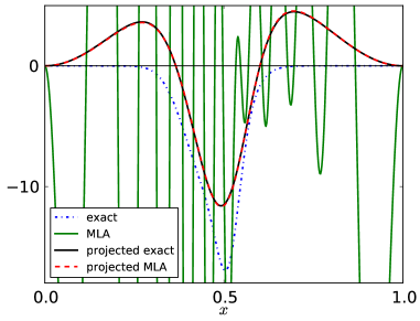
IV.4 Manifold reconstruction using principal component analysis
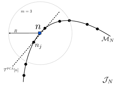
Our aim is to reconstruct locally around a given density , which is assumed to be on the density manifold. A simple approach is to approximate as locally linear, using principal component analysis (PCA) to determine the tangent space empirically from the training densities. This will work as long as there are enough training densities covering the density manifold. First, we define a weighted average density around density :
| (25) |
This generalized average is weighted by the function that only depends on the distance from to , , and . Note that refers to the density evaluated at and not the derivative of with respect to .
The locality of the method comes from the choice of . For standard PCA, the choice is , where is the Heaviside function, and is the distance from to the -th nearest training density. This equally weights the nearest training densities, and ignores all other training densities. This choice was used in Ref. Snyder et al. (2012). Here, we choose a slightly smoother weighting function:
| (26) |
Next, PCA is performed by spectral analysis of the empirical covariance operator Bregler and Omohundro (1994), based on the weighted average value around . We define the centered neighborhood by . In this problem, densities are represented on a grid with points, so let be the vector representation of . The covariance matrix is
| (27) |
with eigendecomposition
| (28) |
The eigenvalues are ordered such that . The eigenvectors are called principal components (PCs), and give the directions of maximum variance in the data. We define the variance lost in keeping PCs as . In this case, there is little to no variance in directions orthogonal to the tangent space of , and maximum variance in directions aligned with the tangent space. Thus, the first PCs form a basis for the tangent space, where is the dimensionality of the density manifold (and tangent space). The projection operator onto this basis is:
| (29) |
The tangent space using PCA is given by
| (30) |
Finally, we choose the PCA approximation to the constraint in Eq. (24) as the squared distance from to tangent plane :
| (31) |
The PCA approximate density manifold is then defined implicitly by . The process is illustrated in Fig. 12. In the next section we develop a projected gradient descent method to solve Eq. (24).
IV.5 Projected gradient descent algorithm
For a given ML approximation to the KE functional,
| (32) |
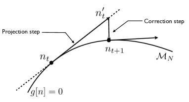
the algorithm to minimize the functional in Eq. (24) to find a constrained optimal density is as follows (see Fig. 13). Choose an initial guess for the density, (e.g., a training density):
-
1.
Evaluate the functional derivative
(33) at .
-
2.
Compute the local PCA projection operator from Eq. (29).
-
3.
Project the functional derivative onto the tangent space (see Fig. 13), and take a step:
(34) where is a constant such that . If convergence is unstable, reduce , trading stability for speed of convergence.
-
4.
To ensure the constraint remains satisfied, we subtract the (weighted) mean of the training densities in the local neighborhood:
(35)
We iterate these steps until convergence is achieved. We measure convergence by setting a maximum iteration step and tolerance threshold. If the total energy difference is smaller than tolerance within max iteration step, the density is converged. If no solution is found, is reduced.
IV.6 Errors on constrained optimal densities
With this new constrained minimization procedure via a projected gradient descent, we solve for the constrained optimal density for each test sample. We report the errors in the total energy and KE relative to the exact density in Table 3. In general, we expect these errors to be worse on the MLA evaluated on exact densities—by roughly a factor of 10. However, errors on constrained optimal densities decrease at the same rate with more training data, so an accuracy of 1 kcal/mol in KE is achieved with 150 training samples for , now on constrained optimal densities. Additionally, errors are of similar magnitude for multiple particles. In the last row of Table 3, we combine the training data from each (100 training densities per value) into one model. This combined MLA gives roughly the same error as each individual model. This is because, due to the locality of the Gaussian kernel, the training densities from each are well separated (orthogonal in feature space) and the individual models are unaffected.
In the projected gradient descent, there are two PCA parameters that must be chosen: , the number of nearest neighbors and , the number of PCs to form the projection operator. Fig. 14 shows the MAE evaluated by the constrained optimal density and variance lost as a function of the number of PCs with .
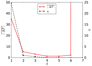
The MAE decreases initially as increases as more PCs capture the local structure of the density manifold. As can be seen, or 5 gives an optimal reconstruction of the tangent space of the manifold. As increases further, the noise that was removed is re-introduced into the projection, causing the gradient descent algorithm to fail. For , many of the constrained searches do not converge. Table 4 reports the errors of the model evaluated on constrained optimal densities for and , giving a rough optimization of the PCA parameters. Although the potential which generates has 9 parameters in this case, we observe that the optimal choice of is only 4. This is because the data used to build the model is only a small fraction of . If we do not sample all relevant directions on , then the model cannot learn the functional derivative in those directions. The PCA projection will compensate by removing those directions. Thus, the effectiveness of our method depends on the sampling on the manifold.
(a)
2
3
4
5
(b)
3
4
5
6
V Conclusion
In this work, we have explored in much greater detail the methods presented in Ref. Snyder et al. (2012), in which ML methods were used to directly approximate the KE of a quantum system as a functional of the electron density, and used this functional in a modified orbital-free DFT to obtain highly accurate self-consistent densities and energies.
We used a simple model as a proof of principle, to investigate how standard methods from ML can be applied to DFT. In particular, we tested a variety of standard kernels used in ML, and have found that the Gaussian kernel gives the lowest errors (the Cauchy kernel also achieves similar performance). All cross validation schemes that were tested gave similar predictions of hyperparameters that achieved low generalization error on the test set. Our results highlight the importance of an appropriate choice of kernel, as some of the kernels tested gave strikingly bad performance. With the construction of the norm that was used in the kernels, the method is basis set independent (as long as a complete basis is used). However, the ML method is capable of learning accurate KEs using a sparse grid (i.e., an incomplete basis). Using a sparse representation for the density without losing accuracy would speed up calculations further. These results warrant further exploration and will be the subject of future work.
We explained the origin of the noise in the functional derivative and developed a constrained search over the density manifold via a modified Euler equation, effectively projecting out the noise. We also introduced a local approximation to the manifold using PCA, and solved for constrained optimal densities using a projected gradient descent algorithm. This worked well for our prototype system, yielding highly accurate constrained optimal energies and densities.
Acknowledgements.
The authors thank for the support from NSF Grant No. CHE-1240252 (JS, KB). KRM thanks the BK21 Plus Program by NRF Korea, DFG and the Einstein Foundation. Correspondence to Li Li and K.-R. Müller.References
- Dirac (1929) Paul Adrien Maurice Dirac, “Quantum mechanics of many-electron systems,” Proceedings of the Royal Society of London. Series A, Containing Papers of a Mathematical and Physical Character 123, 714–733 (1929).
- Kohn (1999) Walter Kohn, “Nobel lecture: Electronic structure of matter-wave functions and density functionals,” Reviews of Modern Physics 71, 1253–1266 (1999).
- Hohenberg and Kohn (1964) P. Hohenberg and W. Kohn, “Inhomogeneous electron gas,” Phys. Rev. B 136, 864–871 (1964).
- Dreizler and Gross (1990) R. M. Dreizler and E. K. U. Gross, Density Functional Theory: An Approach to the Quantum Many-Body Problem (Springer, 1990).
- Thomas (1927) Llewellen H Thomas, “The calculation of atomic fields,” in Mathematical Proceedings of the Cambridge Philosophical Society, Vol. 23 (Cambridge Univ Press, 1927) pp. 542–548.
- Fermi (1928) Enrico Fermi, “Eine statistische methode zur bestimmung einiger eigenschaften des atoms und ihre anwendung auf die theorie des periodischen systems der elemente,” Zeitschrift für Physik 48, 73–79 (1928).
- Teller (1962) Edward Teller, “On the stability of molecules in the thomas-fermi theory,” Reviews of Modern Physics (US) 34 (1962).
- Kohn and Sham (1965) W. Kohn and L. J. Sham, “Self-consistent equations including exchange and correlation effects,” Phys. Rev. 140, A1133–A1138 (1965).
- Becke (1988) A. D. Becke, “Density-functional exchange-energy approximation with correct asymptotic behavior,” Phys. Rev. A 38, 3098–3100 (1988).
- Lee et al. (1988) Chengteh Lee, Weitao Yang, and Robert G. Parr, “Development of the colle-salvetti correlation-energy formula into a functional of the electron density,” Phys. Rev. B 37, 785–789 (1988).
- Perdew et al. (1996) John P. Perdew, Kieron Burke, and Matthias Ernzerhof, “Generalized gradient approximation made simple,” Phys. Rev. Lett. 77, 3865–3868 (1996).
- Karasiev and Trickey (2012) V.V. Karasiev and S.B. Trickey, “Issues and challenges in orbital-free density functional calculations,” Computer Physics Communications 183, 2519 – 2527 (2012).
- Karasiev et al. (2009a) Valentin V. Karasiev, Randy S. Jones, Samuel B. Trickey, and Frank E. Harris, “Recent advances in developing orbital-free kinetic energy functionals,” in New Developments in Quantum Chemistry, edited by José Luis Paz and Antonio J. Hernández (Transworld Research Network, Kerala, India, 2009) pp. 25–54.
- Tran and Wesolowski (2002a) Fabien Tran and Tomasz A. Wesolowski, “Link between the kinetic- and exchange-energy functionals in the generalized gradient approximation,” International Journal of Quantum Chemistry 89, 441–446 (2002a).
- Hung and Carter (2009) Linda Hung and Emily A Carter, “Accurate simulations of metals at the mesoscale: Explicit treatment of 1 million atoms with quantum mechanics,” Chemical Physics Letters 475, 163–170 (2009).
- Hodak et al. (2008) Miroslav Hodak, Wenchang Lu, and J Bernholc, “Hybrid ab initio kohn-sham density functional theory/frozen-density orbital-free density functional theory simulation method suitable for biological systems,” The Journal of chemical physics 128, 014101 (2008).
- Weizsäcker (1935) C.F.v. Weizsäcker, “Zur theorie der kernmassen,” Zeitschrift für Physik 96, 431–458 (1935).
- Wang and Carter (2000) Y.A. Wang and E.A. Carter, “Orbital-free kinetic-energy density functional theory,” in Theoretical Methods in Condensed Phase Chemistry, edited by S.D. Schwartz (Kluwer, NY, 2000).
- Karasiev et al. (to appear) V.V. Karasiev, D. Chakraborty, and S.B. Trickey, “Progress on new approaches to old ideas: Orbital-free density functionals,” in Many-Electron Approaches in Physics, Chemistry, and Mathematics, edited by L. Delle Site and V. Bach (Springer Verlag, Kluwer, NY, to appear).
- Karasiev et al. (2009b) V. V. Karasiev, R. S. Jones, S. B. Trickey, and Frank E. Harris, “Properties of constraint-based single-point approximate kinetic energy functionals,” Phys. Rev. B 80, 245120 (2009b).
- Karasiev et al. (2013) V. V. Karasiev, R. S. Jones, S. B. Trickey, and Frank E. Harris, “Erratum: Properties of constraint-based single-point approximate kinetic energy functionals [phys. rev. b 80, 245120 (2009)],” Phys. Rev. B 87, 239903 (2013).
- Tran and Wesolowski (2002b) Fabien Tran and Tomasz A. Wesolowski, “Link between the kinetic- and exchange-energy functionals in the generalized gradient approximation,” International Journal of Quantum Chemistry 89, 441–446 (2002b).
- Chacón et al. (1985) E. Chacón, J. E. Alvarellos, and P. Tarazona, “Nonlocal kinetic energy functional for nonhomogeneous electron systems,” Phys. Rev. B 32, 7868–7877 (1985).
- García-González et al. (1996) P. García-González, J. E. Alvarellos, and E. Chacón, “Nonlocal kinetic-energy-density functionals,” Phys. Rev. B 53, 9509–9512 (1996).
- García-González et al. (1998) P. García-González, J. E. Alvarellos, and E. Chacón, “Nonlocal symmetrized kinetic-energy density functional: Application to simple surfaces,” Phys. Rev. B 57, 4857–4862 (1998).
- Wang and Teter (1992) Lin-Wang Wang and Michael P. Teter, “Kinetic-energy functional of the electron density,” Phys. Rev. B 45, 13196–13220 (1992).
- Wang et al. (1999) Yan Alexander Wang, Niranjan Govind, and Emily A. Carter, “Orbital-free kinetic-energy density functionals with a density-dependent kernel,” Phys. Rev. B 60, 16350–16358 (1999).
- Xia et al. (2012) Junchao Xia, Chen Huang, Ilgyou Shin, and Emily A. Carter, “Can orbital-free density functional theory simulate molecules?” The Journal of Chemical Physics 136, 084102 (2012).
- Snyder et al. (2012) John C. Snyder, Matthias Rupp, Katja Hansen, Klaus-Robert Müller, and Kieron Burke, “Finding density functionals with machine learning,” Phys. Rev. Lett. 108, 253002 (2012).
- Snyder et al. (2013) John C. Snyder, Matthias Rupp, Katja Hansen, Leo Blooston, Klaus-Robert Müller, and Kieron Burke, “Orbital-free bond breaking via machine learning,” J. Chem. Phys. 139, 224104 (2013).
- Müller et al. (2001) Klaus-Robert Müller, Sebastian Mika, Gunnar Rätsch, Koji Tsuda, and Bernhard Schölkopf, “An introduction to kernel-based learning algorithms,” IEEE Trans. Neural Network 12, 181–201 (2001).
- Kononenko (2001) Igor Kononenko, “Machine learning for medical diagnosis: history, state of the art and perspective,” Artificial Intelligence in medicine 23, 89–109 (2001).
- Huang et al. (2005) Wei Huang, Yoshiteru Nakamori, and Shou-Yang Wang, “Forecasting stock market movement direction with support vector machine,” Computers & Operations Research 32, 2513–2522 (2005).
- Sebastiani (2002) Fabrizio Sebastiani, “Machine learning in automated text categorization,” ACM computing surveys (CSUR) 34, 1–47 (2002).
- Rupp et al. (2012) Matthias Rupp, Alexandre Tkatchenko, Klaus-Robert Müller, and O. Anatole von Lilienfeld, “Fast and accurate modeling of molecular atomization energies with machine learning,” Phys. Rev. Lett. 108, 058301 (2012).
- Hansen et al. (2013) Katja Hansen, Grégoire Montavon, Franziska Biegler, Siamac Fazli, Matthias Rupp, Matthias Scheffler, O. Anatole von Lilienfeld, Alexandre Tkatchenko, and Klaus-Robert Müller, “Assessment and validation of machine learning methods for predicting molecular atomization energies,” Journal of Chemical Theory and Computation 9, 3404–3419 (2013), http://pubs.acs.org/doi/pdf/10.1021/ct400195d .
- Montavon et al. (2013a) Gregoire Montavon, Matthias Rupp, Vivekanand Gobre, Alvaro Vazquez-Mayagoitia, Katja Hansen, Alexandre Tkatchenko, Klaus-Robert Müller, and O Anatole von Lilienfeld, “Machine learning of molecular electronic properties in chemical compound space,” New Journal of Physics 15, 095003 (2013a).
- Pozun et al. (2012) Zachary D. Pozun, Katja Hansen, Daniel Sheppard, Matthias Rupp, Klaus-Robert Müller, and Graeme Henkelman, “Optimizing transition states via kernel-based machine learning,” The Journal of Chemical Physics 136, 174101 (2012).
- Bartók et al. (2010) Albert P. Bartók, Mike C. Payne, Risi Kondor, and Gábor Csányi, “Gaussian approximation potentials: The accuracy of quantum mechanics, without the electrons,” Phys. Rev. Lett. 104, 136403 (2010).
- Hairer et al. (1993) E. Hairer, P. Nørsett, P. Syvert Paul, and G. Wanner, Solving ordinary differential equations I: Nonstiff problems (Springer, New York, 1993).
- Kim et al. (2013) Min-Cheol Kim, Eunji Sim, and Kieron Burke, “Understanding and reducing errors in density functional calculations,” Phys. Rev. Lett. 111, 073003 (2013).
- Lieb (2002) Elliott H Lieb, “Density functionals for coulomb systems,” in Inequalities (Springer, 2002) pp. 269–303.
- Vapnik (1995) V.N. Vapnik, The nature of statistical learning theory (Springer Verlag, New York, 1995).
- Scholkopf et al. (1999) B. Scholkopf, S. Mika, C.J.C. Burges, P. Knirsch, K.-R. Muller, G. Ratsch, and A.J. Smola, “Input space versus feature space in kernel-based methods,” Neural Networks, IEEE Transactions on 10, 1000 –1017 (1999).
- Montavon et al. (2013b) G. Montavon, M. Braun, T. Krueger, and K.-R. Muller, “Analyzing local structure in kernel-based learning: Explanation, complexity, and reliability assessment,” Signal Processing Magazine, IEEE 30, 62–74 (2013b).
- Schölkopf and Smola (2002) Bernhard Schölkopf and Alexander Smola, Learning with Kernels (MIT Press, Cambridge, 2002).
- Mercer (1909) James Mercer, “Functions of positive and negative type, and their connection with the theory of integral equations,” Philosophical transactions of the royal society of London. Series A, containing papers of a mathematical or physical character 209, 415–446 (1909).
- Aronszajn (1950) Nachman Aronszajn, “Theory of reproducing kernels,” Transactions of the American mathematical society 68, 337–404 (1950).
- Schölkopf et al. (1998) B. Schölkopf, A. Smola, and K.R. Müller, “Nonlinear component analysis as a kernel eigenvalue problem,” Neural computation 10, 1299–1319 (1998).
- Hastie et al. (2009) Trevor Hastie, Robert Tibshirani, and Jerome Friedman, The Elements of Statistical Learning: Data Mining, Inference, and Prediction, 2nd ed. (Springer, New York, 2009).
- Smola et al. (1998) A.J. Smola, B. Schölkopf, and K.-R. Müller, “The connection between regularization operators and support vector kernels,” Neural Networks 11, 637–649 (1998).
- Rupp et al. (2007) Matthias Rupp, Ewgenij Proschak, and Gisbert Schneider, “Kernel approach to molecular similarity based on iterative graph similarity,” JChemInfModel 47, 2280–2286 (2007).
- Zien et al. (2000) Alexander Zien, Gunnar Rätsch, Sebastian Mika, Bernhard Schölkopf, Thomas Lengauer, and K-R Müller, “Engineering support vector machine kernels that recognize translation initiation sites,” Bioinformatics 16, 799–807 (2000).
- Braun et al. (2008) M.L. Braun, J.M. Buhmann, and K.-R. Müller, “On relevant dimensions in kernel feature spaces,” Journal of Machine Learning Research 9, 1875–1908 (2008).
- Poggio et al. (2001) Tomaso Poggio, Sayan Mukherjee, Ryan Rifkin, Alexander Rakhlin, and Alessandro Verri, b, Tech. Rep. AI Memo 2001-011, CBCL Memo 198 (Massachusetts Institute of Technology, 2001).
- Amari et al. (1997) S-I Amari, N Murata, K-R Müller, M Finke, and HH Yang, “Asymptotic statistical theory of overtraining and cross-validation,” IEEE Transactions on Neural Networks 8, 985–996 (1997).
- Lemm et al. (2011) S. Lemm, B. Blankertz, T. Dickhaus, and K.-R. Müller, “Introduction to machine learning for brain imaging,” Neuroimage 56, 387–399 (2011).
- Bregler and Omohundro (1994) Christoph Bregler and Stephen M Omohundro, Surface learning with applications to lipreading (International Computer Science Institute, 1994).