Weak Limit of the 3-State Quantum Walk on the Line

Abstract

We revisit the one dimensional discrete time quantum walk with 3-states and the Grover coin, the simplest model that exhibits localization in a quantum walk. We derive analytic expressions for the localization and a long-time approximation for the entire probability density function (PDF). We also connect the time-averaged approximation of the PDF found by Inui et. al. to a spatial average of the walk. We show that this smoothed approximation predicts moments of the real PDF accurately.

Figure 1: The one dimensional quantum walk with a three dimensional coin. The matrices $\mathcal{P}$, $\mathcal{Q}$ and $\mathcal{R}$ facilitate a right hop, a left hop, or no change in position.

I Introduction

Quantum walks have been the subject of research for the past 20 years Kempe (2003); Konno (2008); Venegas-Andraca (2012); Portugal (2013). They were originally proposed as a description for quantum transport in a one dimensional system Aharonov et al. (1993); Meyer (1996). However, quantum walks soon received considerable prominence as the driving dynamics behind quantum search algorithms Grover (1997); Farhi and Gutmann (1998), leading to many systematic studies of their asymptotic properties Aharonov et al. (2001); Ambainis et al. (2001); Bach et al. (2004); Childs and Goldstone (2004). Other applications, such as to the graph isomorphism problem Ambainis (2003); Rudinger et al. (2013), further increased the interest. The realization of their capability for general quantum computations Childs (2009); Lovett et al. (2010) suggests that understanding quantum walks is a quest for a better understanding of quantum computing itself.

Due to its wealth of possible parameters, the discrete-time quantum walk has been studied extensively. From the basic properties of the simplest possible quantum walk on the one dimensional line Ambainis et al. (2001), time-dependent coins Banuls et al. (2006) and site-dependent coins Shikano and Katsura (2010) are just some of the many extensions that have been investigated. In this paper, we revisit the one-dimensional quantum walk with the three-dimensional Grover coin, previously considered by Inui et. al. Inui et al. (2005). They discussed a variation of the walk on the line, where the walker can remain on the site during a time step, and found interesting differences to the case of a two-dimensional coin. Most notably, there is a finite probability that the quantum walk strongly localizes around the initial site, as previously found on square lattices Inui et al. (2004). In fact, this model is the simplest model exhibiting localization, a distinctly quantum effect entirely absent in the corresponding classical random walks, that becomes a generic features of discrete-time quantum walks on higher-dimensional structures Portugal (2013); Boettcher et al. (3369); Ide et al. (2014). Here, we extend the findings of Ref. Inui et al. (2005) by analytic expressions for this localization, calculate the weak limit of the probability density function (PDF), and show its equivalence to a spatial average over a local neighborhood. We provide explicit expressions for general initial conditions present on one site, study the convergence, and compare our analytic predictions for moments with those from numerical simulations.

The paper is organized as follows. In Sec. II, we review the basics for the 3-state quantum walk on the line. In Sec. III we show how the long-time behavior can be obtained, with an accurate description of the localization and an approximation for the spreading front. In Sec. IV, we introduce an approximation that leads to a smoothed PDF, corresponding to a spatial as well as temporal average. Finally, in Sec. V, we summarize our findings.

II The 3-State Quantum Walk

In the common description of the discrete-time quantum walk, every time step consists of two parts. First, the coin (operator) is applied to the internal degree of freedom (coin state) at every site. This is followed by the shift operator, translating components of the coin state to neighboring sites. Here, we study the case of the one dimensional quantum walk with a three dimensional coin space, driven by the Grover Coin

$$\mathcal{C}=\frac{1}{3}\begin{bmatrix}-1&2&2\\ 2&-1&2\\ 2&2&-1\end{bmatrix}\,.$$ (1)

Our convention for the shift operation is the following: the first component is moved to the left, the third component to the right, while the second one remains on the site. The matrices $\mathcal{P}$, $\mathcal{Q}$, and $\mathcal{R}$ (see Fig. 1) combine both steps into a single operation, leading to the master equation describing the time evolution at any site $n$,

$$\left|{\psi_{n}^{t+1}}\right\rangle=\mathcal{P}\left|{\psi_{n-1}^{t}}\right\rangle+\mathcal{Q}\left|{\psi_{n+1}^{t}}\right\rangle+\mathcal{R}\left|{\psi_{n}^{t}}\right\rangle,$$ (2)

with

$$\mathcal{P}=\begin{bmatrix}0&0&0\\ 0&0&0\\ \frac{2}{3}&\frac{2}{3}&-\frac{1}{3}\end{bmatrix},\,\mathcal{Q}=\begin{bmatrix}-\frac{1}{3}&\frac{2}{3}&\frac{2}{3}\\ 0&0&0\\ 0&0&0\end{bmatrix}\,,\mathcal{R}=\begin{bmatrix}0&0&0\\ \frac{2}{3}&-\frac{1}{3}&\frac{2}{3}\\ 0&0&0\end{bmatrix}\,.$$

For simplicity, we assume the inital conditions are only non-zero on site $n=0$, i.e. ,

$$\left|{\psi_{n}^{0}}\right\rangle=\delta_{n,0}\cdot\left|{\psi_{0}^{0}}\right\rangle\,.$$ (3)

These equations can be solved by a Fourier transform,

$$\left|{\tilde{\psi}^{t}}\right\rangle=\sum_{n=-\infty}^{\infty}\mathrm{e}^{-\mathrm{i}\cdot k\cdot n}\cdot\left|{\psi^{t}_{n}}\right\rangle\,.$$ (4)

From here on, a tilde indicates quantities with a $k$-dependence, which we will not explicitly show. Applying Eq. (4) to Eq. (2) yields the master equation in Fourier space:

$$\left|{\tilde{\psi}^{t+1}}\right\rangle=\underbrace{\frac{1}{3}\begin{bmatrix}-\kappa&2\kappa&2\kappa\\ 2&-1&2\\ 2\kappa^{-1}&2\kappa^{-1}&-\kappa^{-1}\end{bmatrix}}_{:=\tilde{C}}\cdot\left|{\tilde{\psi}^{t}}\right\rangle\,,$$ (5)

where $\kappa=\mathrm{e}^{\mathrm{i}\cdot k}$. The solution to this equation

$$\left|{\tilde{\psi}^{t}}\right\rangle=\tilde{\mathcal{C}}^{t}\cdot\left|{\psi_{0}^{0}}\right\rangle$$ (6)

can be found by computing the eigenvalue decomposition

$$\mathcal{T}^{-1}\cdot\tilde{\mathcal{C}}\cdot\mathcal{T}=\begin{bmatrix}\tilde{\lambda}_{1}&0&0\\ 0&\tilde{\lambda}_{2}&0\\ 0&0&\tilde{\lambda}_{3}\end{bmatrix}\,.$$ (7)

One eigenvalue is purely real, $\tilde{\lambda}_{1}=1$, whereas the other two obey

$$\lambda_{2,3}=\mathrm{e}^{\pm\mathrm{i}\tilde{\omega}}\quad\text{, and}\quad\cos\left(\tilde{\omega}\right)=-\frac{2}{3}-\frac{\cos(k)}{3}\,.$$ (8)

The $t^{\text{th}}$ power of $\tilde{\mathcal{C}}$ can then be expressed as

$$\tilde{\mathcal{C}}^{t}=\tilde{\mathcal{M}_{1}}+\tilde{\lambda}_{2}^{t}\cdot\tilde{\mathcal{M}_{2}}+\tilde{\lambda}_{3}^{t}\cdot\tilde{\mathcal{M}_{3}}\,.$$ (9)

A representation of $\mathcal{T}$ and the $\tilde{\mathcal{M}}$ matrices can be found in the supplementary Mathematica notebook sup . In the end, the real space solution is obtained by performing the inverse Fourier transform

$$\left|{\psi_{n}^{t}}\right\rangle=\frac{1}{2\pi}\intop_{-\pi}^{\pi}\mathrm{e}^{\mathrm{i}\cdot n\cdot k}\cdot\left|{\tilde{\psi}^{t}}\right\rangle\,\mathrm{d}k\,.$$ (10)

In the next section, we perform an asympotic approximation in the long-time limit to find the leading behaviour of the PDF.

III Long-Time Approximation

In this section, we evaluate Eq. (10) in the limit of $t\to\infty$. First, we compute the time independent part of $\left|{\psi_{n}^{t}}\right\rangle$ that manifests itself as localization. As a test, we compare our result with numerical simulations. Afterwards, we use the method of stationary phase to find an approximation for the remaining, time dependent part.

III.1 The Stationary Distribution

One can see from Eq. (9) that a time-independent component of $\left|{\tilde{\psi}^{t}}\right\rangle$ can exist due to the constant eigenvalue of $\tilde{\mathcal{C}}$. The inverse Fourier transform of this part can be computed exactly by employing the residue theorem. Note that the corresponding integral for this part following from equations (9) and (10), in terms of $\kappa$ reads

$$\left|{\psi_{n}^{\infty}}\right\rangle=\underbrace{\frac{1}{2\pi\mathrm{i}}\ointop_{\left|{\kappa}\right|=1}\kappa^{n-1}\mathcal{\tilde{M}}_{1}\,\mathrm{d}\kappa}_{:=\,\mathcal{U}_{1}(n)}\cdot\left|{\psi_{0}^{0}}\right\rangle\,.$$ (11)

The details of this calculation can be found in Appendix A, but the essential observation is that all components of $\tilde{\mathcal{M}}_{1}$ share the same poles,

$$\kappa_{\pm}=-5\pm 2\sqrt{6},$$ (12)

of which only $\kappa_{+}$ is inside the unit circle. For $n\leq 0$, there is an additional pole at $\kappa=0$. By straightforward calculations, we find an expression for $\mathcal{U}_{1}(n)$ for different regimes for $n$:

$$\mathcal{U}_{1}(n<0) =\frac{\kappa_{-}^{n}}{\sqrt{6}}\begin{bmatrix}1&-2-\sqrt{6}&-5-2\sqrt{6}\\ -2+\sqrt{6}&-2&-2-\sqrt{6}\\ -5+2\sqrt{6}&-2+\sqrt{6}&1\\ \end{bmatrix}$$

$$\mathcal{U}_{1}(n=0) =\frac{1}{\sqrt{6}}\begin{bmatrix}1&-2+\sqrt{6}&-5+2\sqrt{6}\\ -2+\sqrt{6}&-2+\sqrt{6}&-2+\sqrt{6}\\ -5+2\sqrt{6}&-2+\sqrt{6}&1\\ \end{bmatrix}$$ (13)

$$\mathcal{U}_{1}(n>0) =\frac{\kappa_{+}^{n}}{\sqrt{6}}\begin{bmatrix}1&-2+\sqrt{6}&-5+2\sqrt{6}\\ -2-\sqrt{6}&-2&-2+\sqrt{6}\\ -5-2\sqrt{6}&-2-\sqrt{6}&1\\ \end{bmatrix}$$

At first, the case distinction in the sign of $n$ seems counterintuitive, but the comparison to the numerics in Fig. LABEL:fig:localization_comparison reveals the possibility of an asymmetric localization around the initial site.

To obtain the stationary PDF, we calculate

$$p_{1}(n)=\langle\psi_{n}^{\infty})|\psi_{n}^{\infty}\rangle=\langle\psi_{0}^{0}|U_{1}^{\dagger}(n)U_{1}(n)|\psi_{0}^{0}\rangle\,.$$ (14)

For general initial condition, $p_{1}(n)$ still contains the case distinction in $n$, but the localization only at the initial site for arbitrary $\left|{\psi_{0}^{0}}\right\rangle=(\alpha,\beta,\gamma)^{T}$, for example, reads:

$$\left(\bar{\alpha},\bar{\beta},\bar{\gamma}\right)\cdot\mathcal{U}_{1}^{\dagger}(0)\cdot\mathcal{U}_{1}(0)\cdot\begin{pmatrix}\alpha\\ \beta\\ \gamma\end{pmatrix}=\left(5-2\sqrt{6}\right)\cdot$$ (15)

$$\qquad~{}~{}((2\alpha+\beta)\bar{\alpha}+(\alpha+\beta+\gamma)\bar{\beta}+(\beta+2\gamma)\bar{\gamma})\,,$$

which coincides with the result in Ref. Inui et al. (2005).

We point out that the stationary PDF always decays exponentially away from the initial site as $p_{1}(n)\sim\kappa_{+}^{2\left|{n}\right|}$ independent of the initial condition, even though the proportionality constant might differ from positive to negative $n$. The initial condition $\left|{\psi_{0}^{0}}\right\rangle\propto(1,-2,1)$ is a non-generic case where the localization completely vanishes. There exists also a whole family,$\left|{\psi_{0}^{0}}\right\rangle\propto(-a\cdot(1+\kappa_{\pm})/2-b\cdot\kappa_{\pm},a,b)$ with $a,b\in\mathbb{R}$, where the localization vanishes for positive (negative) $n$ while still exponentially decaying for negative (positive) values.

To show that our calculations describe the localized part comprehensively, we compare to a long simulation of a system, where the system is large enough that the finite size has no influence on the PDF near the initial site at the end of the simulation. The system starts with different initial conditions and evolves for $2^{20}$ time steps. In the end, the final probabilities at sites around the origin are recorded. Figure LABEL:fig:localization_comparison shows the comparison between evaluating Eq. (14) and the simulation. To demonstrate the asymmetry, we choose 3 particular initial conditions.

This rapid decay renders estimating $p_{1}(n)$ with simulations for $\left|{n}\right|>12$ problematic. The values range over 30 orders of magnitude, challenging the machine precision used in the simulations. Furthermore, the time to converge to $p_{1}(n)$ grows exponentially with $n$, as we will see, which restricts the numerical evaluation, as system size would have to grow exponentially as well.

III.2 Approximating the Time-Dependent Integrals

After solving the time independent part analytically, we have to resort to approximations for the time dependent part of $\left|{\tilde{\psi}^{t}}\right\rangle$ in the limit $t\to\infty$. In analogy to Eq. (11), we define

$$\mathcal{U}_{2,3}(t,n)=\frac{1}{2\pi}\intop_{-\pi}^{\pi}\mathrm{e}^{\mathrm{i}\cdot k\cdot n}\tilde{\mathcal{M}}_{2,3}\cdot\tilde{\lambda}_{2,3}^{t}\,\mathrm{d}k\,,$$ (16)

such that the sum $\mathcal{U}_{1}+\mathcal{U}_{2}+\mathcal{U}_{3}=\tilde{\mathcal{C}}^{t}$ expresses the full time evolution. By introducing the ”velocity” $v$ via

$$n=v\cdot t$$ (17)

and using Eq. (8), we write the integrals as

$$\frac{1}{2\pi}\intop_{-\pi}^{\pi}\tilde{f}(k)\cdot\mathrm{e}^{\mathrm{i}t\cdot\left(vk\pm\tilde{\omega}\right)}\,\mathrm{d}k\,.$$

where the function $\tilde{f}$ represents the different (slowly-varying) elements of the $\tilde{\mathcal{M}}$ matrices.

This form is known as a generalized Fourier integral Bender and Orszag (1999), and the leading, long-time behavior can be found by the method of stationary phase. The method assumes that the main contribution to the integral stems from a small region of $k$ around an extremal value of $(vk\pm\tilde{\omega})$, say $k^{*}$. Expanding the exponent to second order and replacing the function $\tilde{f}(k)$ by $\tilde{f}(k^{*})$ yields a solvable Gaussian integral. A more detailed discussion can be found in Appendix B.

In this approximation, $\tilde{\mathcal{C}}^{t}$ will contain the constant terms from $\mathcal{U}_{1}$ and terms proportional to $t^{-1/2}$ that further oscillate both in space and in time. In their full extend, these terms are too complex to write down here, but easily used to compute numerical values for specific initial conditions. The supplementary Mathematica notebook contains an applet that shows the approximation for interactive initial conditions sup .

Figure LABEL:fig:comparison_data_pred_p_vs_n_1 shows the PDF for a specific initial condition as a function of the site index $n$ for a fixed time $t$. To show the quality of the approximation, we also show the relative difference

$$\varepsilon_{r}=\frac{2\cdot\left|{p_{s}(n,t)-p_{a}(n,t)}\right|}{p_{s}(n,t)+p_{a}(n,t)}$$ (18)

between the simulation $p_{s}$ and the asymptotic expression $p_{a}$. Note that prediction and simulation are indistinguishable on this scale. The quality of the prediction remains excellent for general (complex and asymmetric) initial conditions $\left|{\psi_{0}^{0}}\right\rangle$.

The approximation can also be used for a fixed $n$ as a function of $t$, as demonstrated in Fig. LABEL:fig:comparison_data_pred_p_vs_t_1 for the initial site. The plot displays a short short sequence of a time series at large $t$. Again, simulation and asymptotic approximation are indistinguishable on this scale.

To better understand the quality of the approximation, we plot the relative difference in the bottom part of Fig. LABEL:fig:comparison_data_pred_p_vs_t_1. The data suggests, surprisingly, that the error of the approximation decays as $\sim t^{-3/2}$. This would imply that the method of stationary phase correctly predicts the leading behavior to order $t^{-1}$. This cannot be expected a priory, because the next order, obtainable with the method of steepest descent, may yield terms of that order for $\tilde{\mathcal{C}}^{t}$. Those should generate terms of the same magnitude in the PDF due to the constant eigenvalue. The data here suggests that such terms cancel out.

IV Weak Limit Distribution

In the previous section, we found that the method of stationary phase yields a good approximation to the evolution of the quantum walk for sufficiently large times. It also became obvious that the PDF oscillates as a function of both $n$ and $t$, especially close to the moving front, near $\left|v\right|\lesssim 1/\sqrt{3}$. In this section, we find a smooth approximation known as the weak limit Grimmett et al. (2004). We demonstrate that it yields a proper PDF, study the convergence towards it, and show that the walk spreads ballistically for all initial conditions.

IV.1 Properties and Implications

Following Ambainis et. al. Ambainis et al. (2001), we can separate out the rapidly oscillating part of Eq. (9). If we ignore the localized part for a moment, the corresponding distribution, which we will call $p_{avg}(n,t)$, can be found via

$$p_{avg}(n,t)=\left\langle{\psi_{0}^{0}}\right|\left(\mathcal{U}_{2}^{\dagger}\cdot\mathcal{U}_{2}+\mathcal{U}_{3}^{\dagger}\cdot\mathcal{U}_{3}\right)\left|{\psi_{0}^{0}}\right\rangle$$ (19)

This expression seems ad hoc, but contains all non-oscillating terms from the full approximation. This corresponds to a temporal average at a specific site, assuming that the rapidly oscillating phase factors lead to a negligible contribution to the inverse Fourier transform (according to Riemann-Lebesgue). We argue that this also corresponds to a local spatial average at fixed $t$, because as $t\to\infty$ a small change in $n$ will only lead to an small change in $v$, such that the non-oscillating contribution should be the same in a neighborhood around a point that is reasonably small compared to $t$. This average also smoothes out the spatial oscillations of the PDF. In fact, we will use a spatial average to numerically predict $p_{avg}$.

Inserting the expressions for $\mathcal{U}_{2,3}(n,t)$, we find the matrix

$$\mathcal{U}_{2}^{\dagger}\cdot\mathcal{U}_{2}+ \mathcal{U}_{3}^{\dagger}\cdot\mathcal{U}_{3}=\frac{1}{\pi t\sqrt{2(1-3v^{2})}~{}(1-v^{2})}\cdot$$ (20)

$$\begin{bmatrix}(1-v)^{2}&2v(1-v)&1-5v^{2}\\ 2v(1-v)&2-2v^{2}&-2v(1+v)\\ 1-5v^{2}&-2v(1+v)&(1+v)^{2}\end{bmatrix}$$

valid for all $n$ subjected to $\left|{n}\right|/t<1/\sqrt{3}$. Outside this interval, $p_{avg}(n,t)\equiv 0$. The dependency on $n$ is implicit through $v=n/t$. For a specific initial condition, a comparison between the numerical simulation and the analytic prediction can be found in Fig. LABEL:fig:avg_pdf_comparison1.

Our definition of $p_{avg}(n,t)$ closely relates to the weak limit proven by Grimmett et. al. Grimmett et al. (2004). Note that $p_{avg}(n,t)/t$ only depends on $v$ which corresponds to $f(y)$ in their notation. They show that every quantum walk on regular lattices exhibits this convergence, for example, see Eq. (20) in Ref. Grimmett et al. (2004).

In the long-time limit, we can tread $v=n/t$ as a continuous variable. Hence, we approximate probabilities

$$p(n_{-}\leq n\leq n_{+},t)=\sum_{n=n_{-}}^{n_{+}}p(n,t)$$

by integrals of the form

$$p(a\ \leq v\leq b,t)=\intop_{a}^{b}p_{avg}(v\cdot t,t)\cdot t\,\mathrm{d}v\,.$$

Here $a=n_{-}/t$ and $b=n_{+}/t$. By using the convergence of $p_{avg}(v\cdot t,t)\cdot t$ to a stationary distribution solely depending on $v$, we conclude that the spreading is always ballistic. In this continuous limit, the localized part remains concentrated at the initial site, and

$$p_{1}(v\cdot t)\cdot t\to\left\langle{\psi_{0}^{0}}\right|\begin{pmatrix}\frac{1}{\sqrt{6}}&1-\sqrt{\frac{2}{3}}&2-\frac{5}{\sqrt{6}}\\ 1-\sqrt{\frac{2}{3}}&1-\sqrt{\frac{2}{3}}&1-\sqrt{\frac{2}{3}}\\ 2-\frac{5}{\sqrt{6}}&1-\sqrt{\frac{2}{3}}&\frac{1}{\sqrt{6}}\\ \end{pmatrix}\left|{\psi_{0}^{0}}\right\rangle\,\delta(v)$$ (21)

characterizing the localization within the weak limit. Some algebra reveals that

$$\sum_{n=-\infty}^{\infty}p_{1}(n)+\intop_{-1/\sqrt{3}}^{1/\sqrt{3}}p_{avg}(v\cdot t,t)\cdot t~{}\mathrm{d}v=1\,,$$ (22)

i.e., our approximation actually yields a proper PDF. Connecting once more with Ref. Inui et al. (2004), if the system starts in one of the three initial states $(1,0,0)$, $(0,1,0)$, and $(0,0,1)$ each with probability $1/3$, we rediscover:

$$p(v,t)\approx\frac{1}{3}\,\delta(v)+\frac{4}{3\pi\cdot(1-v^{2})\cdot\sqrt{2-6v^{2}}}\,.$$

But observe that generically the numerator of the second term is quadratic in $v$ rather than just a constant, as can be seen from Eq. (20). As an example, we utilize $p_{avg}(n,t)$ to approximate the second moment of the PDF. Figure LABEL:fig:second_moment shows a comparison between the approximation and numerical simulations. The details of the calculation are in Appendix C, but the main result is that the second moment always grows $\sim t^{2}$ regardless of the initial condition, see Eq. (28). This means, only the PDF’s shape can be influenced by $\left|{\psi_{0}^{0}}\right\rangle$, but not the asymptotic scaling of its spread.

In principle, we can approximate every moment, but the quality declines for higher moments. Those depend stronger on sites farther away from the initial site where the accuracy is worse.

(a)	(b)
(c)	(d)

Figure 7: The numerically observed probabilities (blue dots), the weak-limit approximation $p_{1}(n)+p_{avg}$ (orange line), and corresponding envelopes from the long time approximation (black lines). For the upper panels, it is $\left|{\psi_{0}^{0}}\right\rangle\propto(0,\mathrm{i},1)^{T}$; for the lower ones, it is $\left|{\psi_{0}^{0}}\right\rangle\propto(1,0,-1)^{T}$. The left panels refer to the initial site, whereas the right ones to $n=512$, to contrast sites with and without significant localization. Note the difference in scaling with time, depending on the initial conditions. The insets depict a zoom for large times on the same $t$-scale. For the data in panel (c), there is no prediction from the method of stationary phase, because for $n=0$ all available orders cancel. However, from the formulas we know that the envelope should scale $\sim t^{-3/2}$, as support by the numerical data.

IV.2 Convergence

In the previous sections, we have shown that the 3-state quantum walk on the line is well described by a time independent, localized part, and a ballistically moving front that can be approximated by a smooth PDF. In this section, we investigate, how fast the error of this approximation decays with time.

From the method of stationary phase, we already identified that the localization originates from the $\mathcal{U}_{1}^{\dagger}\cdot\mathcal{U}_{1}$ term, whereas $p_{avg}$ stems from $\mathcal{U}_{2}^{\dagger}\cdot\mathcal{U}_{2}+\mathcal{U}_{3}^{\dagger}\cdot\mathcal{U}_{3}$. We group the missing terms of the approximation into two functions:

$$q_{1} =\left\langle{\psi_{0}^{0}}\right|\mathcal{U}_{1}^{\dagger}\cdot(\mathcal{U}_{2}+\mathcal{U}_{3})+(\mathcal{U}_{2}+\mathcal{U}_{3})^{\dagger}\cdot\mathcal{U}_{1}\left|{\psi_{0}^{0}}\right\rangle$$ (23)

$$q_{avg} =\left\langle{\psi_{0}^{0}}\right|\mathcal{U}_{2}^{\dagger}\cdot\mathcal{U}_{3}+\mathcal{U}_{3}^{\dagger}\cdot\mathcal{U}_{2}\left|{\psi_{0}^{0}}\right\rangle$$ (24)

These functions are not non-negative quantities, hence cannot be interpreted as probabilities. In fact, both functions oscillate and average to zero. As Grimmet et. al. Grimmett et al. (2004) already pointed out, the convergence to the smooth probability function depends in general on the initial conditions. With our approximation, we can determine the slowest convergence rate.

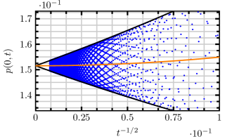
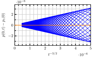
From the formulas in the supplementary material sup , we see that the leading order of $q_{1}$ generically is $\sim t^{-1/2}$. By choosing special initial condition, one can cancel this term, and achieve a faster convergence $\sim t^{-3/2}$. This term dominates for small $n$, but is exponentially suppressed for large $n$. In that case $q_{avg}\gg q_{1}$ and a different convergence rate is possible. In fact for $n\gg 1$, the deviation from the smooth PDF decay at least $\sim t^{-3}$, for particular initial conditions even $\sim t^{-5}$.

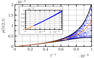
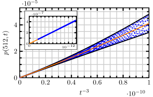
Figure 7 illustrates our findings. It shows the convergence towards $p_{1}(0)+p_{avg}(0,t)$ for two different initial conditions at two different sites. The smooth PDF is represented by the orange line. The envelopes (black lines) are derived from Eqs. (23-24) depending on the site.

Our calculations enable us to make statements about the convergence of the PDF towards the limiting distribution. We have already seen, that the oscillations around the stationary value at the initial site decay $\sim t^{-1/2}$. This was due to the contribution of $\mathcal{U}_{1}(n)$. But for sites sufficiently far away from the initial site, this term becomes exponentially small, and the asymptotic behavior changes. The right panels of Fig. 7 present data similarly to the left, but for $n=512$. By changing the $x$-axis to $t^{-1}$, it is evident from the inset that $p(512,t)\sim t^{-1}$ for sufficiently large times. This corresponds to the stationary distribution itself. By computing the envelope, we find that the next order correction vanishes $\sim t^{-3}$, resulting in a correction $\mathcal{O}(t^{-2})$ for the stationary distribution.

V Conclusion

We studied the 3-state quantum walk on the line in the long time limit using the method of stationary phase. We found explicit formulas for the localization, and found interesting cases where it is only zero for either positive or negative site indices. We showed how the weak limit of the PDF can be interpreted as an time average at a fixed site, or as a spatial average for a fixed $t$. We used the latter interpretation to demonstrate the good agreement between the asymptotic approximation and long time simulations. We applied the smooth, approximative PDF to show that the quantum walk always spreads ballistically for all initial conditions. Finally, we studied the convergence towards this smooth description. We identified the generic convergence rate depending on the site index, and pointed out that other initial conditions only converge faster.

VI Acknowledgments

We gratefully acknowledge helpful discussions with R. Portugal. This work was supported by DMR-grant #1207431 from the NSF.

Appendix A The stationary probability distribution

The non-trivial limit of the PDF as $t\to\infty$ is purely determined by the $\kappa$-independent eigenvalue of $\tilde{\mathcal{C}}$ in Eq. (7). To find this “stationary state”, we evaluate the definition of $\mathcal{U}_{1}$ in Eq. (11). For this calculation, we do not have to resort to any approximation, but can solve the integrals analytically by applying the residue theorem. As already mentioned in the text, all components share the two poles

$$\kappa_{\pm}=-5\pm 2\sqrt{6}$$

of which only $\kappa_{+}$ lies inside the unit circle. Depending on $n$, there is an additional pole at $\kappa=0$. After some simple algebra, we find

$$\mathcal{U}_{1}(n) =\kappa_{+}^{n}\begin{bmatrix}\frac{1}{\sqrt{6}}&1-\sqrt{\frac{2}{3}}&2-\frac{5}{\sqrt{6}}\\ -1-\sqrt{\frac{2}{3}}&-\sqrt{\frac{2}{3}}&1-\sqrt{\frac{2}{3}}\\ -2-\frac{5}{\sqrt{6}}&-1-\sqrt{\frac{2}{3}}&\frac{1}{\sqrt{6}}\\ \end{bmatrix}$$ (25)

$$\kern 28.45274pt+\mathop{\mathrm{Res}}\limits_{\kappa=0}(\kappa^{n-1}\cdot\tilde{\mathcal{M}}_{1})$$

Please refer to the supplementary material for the full expression of $\tilde{\mathcal{M}}_{1}$ sup . The last term is only non-zero if $n\leq 0$ and counteracts the divergence of $\kappa_{+}^{n}$ as $n\to-\infty$. All residues are of the Form

$$\mathop{\mathrm{Res}}\limits_{\kappa=0}\left(\frac{a\kappa^{m}}{1+10\kappa+\kappa^{2}}\right)\,.$$

To calculate the residue, note that with partial fractions

$$\frac{1}{1+10\kappa+\kappa^{2}} =\frac{1}{4\sqrt{6}}\left[\frac{1}{\kappa_{-}-\kappa}-\frac{1}{\kappa_{+}-\kappa}\right]$$

$$=\frac{1}{4\sqrt{6}}\left[\sum_{k=0}^{\infty}\frac{\kappa^{k}}{\kappa_{-}^{k+1}}-\sum_{k=0}^{\infty}\frac{\kappa^{k}}{\kappa_{+}^{k+1}}\right]\,.$$

With this representation, we find

$$\mathop{\mathrm{Res}}\limits_{\kappa=0} \left(\frac{a\kappa^{m}}{1+10\kappa+\kappa^{2}}\right)=\frac{a}{2\pi\mathrm{i}}\ointop\kappa^{m}\frac{1}{1+10\kappa+\kappa^{2}}\,\mathrm{d}\kappa$$

$$=\frac{a}{4\sqrt{6}}\sum_{k=0}^{\infty}\left(\kappa_{-}^{-k-1}-\kappa_{+}^{-k-1}\right)\cdot\underbrace{\frac{1}{2\pi\mathrm{i}}\ointop\kappa^{m+k}\mathrm{d}\kappa}_{=\delta_{-1,m+k}}$$

$$=\frac{a}{4\sqrt{6}}\left[\kappa_{-}^{m}-\kappa_{+}^{m}\right]\,.$$

Plugging this result into Eq. (25), yields Eq. (13).

Appendix B Approximation for long times

The inverse Fourier transform reads

$$\left|{\psi_{n}^{t}}\right\rangle =\left(\frac{1}{2\pi}\intop_{-\pi}^{\pi}\mathrm{e}^{\mathrm{i}\cdot n\cdot k}\cdot\tilde{\mathcal{C}}^{t}\,\mathrm{d}k\right)\cdot\left|{\psi_{0}^{0}}\right\rangle$$

$$=\left[\mathcal{U}_{1}(n)+\mathcal{U}_{2}(n,t)+\mathcal{U}_{3}(n,t)\right]\cdot\left|{\psi_{0}^{0}}\right\rangle\,,$$

We have already seen how $\mathcal{U}_{1}(n)$ emerges from the constant eigenvalue, and how it can be calculated explicitly. For the evaluation of (16), we have to resort to an asymptotic analysis for $t\to\infty$. Note that the integrals can be written as

$$\frac{1}{2\pi}\intop_{-\pi}^{\pi}f(k)\mathrm{e}^{\mathrm{i}\cdot n\cdot k\pm\mathrm{i}\cdot t\cdot\tilde{\omega}}~{}\mathrm{d}k$$

where $f(k)$ represents the components of $\tilde{\mathcal{M}}_{2,3}$. Before we can apply the method, we introduce the parameter $v$, see Eq. (17). This allows us to write the integrals in the form

$$\frac{1}{2\pi}\intop_{-\pi}^{\pi}f(k)\mathrm{e}^{\mathrm{i}\cdot t\cdot\left(v\cdot k\pm\omega(k)\right)}~{}\mathrm{d}k:=\frac{1}{2\pi}\intop_{-\pi}^{\pi}f(k)\mathrm{e}^{\mathrm{i}\cdot t\cdot\rho(k)}~{}\mathrm{d}k$$

The idea is now to expand $\rho(k)$ around any extrema $k^{*}$ to second order:

$$\rho(k)=\rho(k^{*})+\frac{1}{2}\rho^{\prime\prime}(k^{*})(k-k^{*})^{2}+\mathcal{O}\left((k-k^{*})^{3}\right)\,.$$

For $t\to\infty$, this captures the main contribution around these points of stationary phase, and everything else is exponentially suppressed. This requires $f(k^{*})\neq 0$ which holds for all integrals considered here. Within this scheme the integral is approximated by

$$\int f(k)\mathrm{e}^{\mathrm{i}\cdot t\cdot\rho(k)}~{}\mathrm{d}k\approx f(k^{*})\mathrm{e}^{\mathrm{i}\cdot t\cdot\rho(k^{*})}\int\mathrm{e}^{\frac{\mathrm{i}\cdot t\cdot\rho^{\prime\prime}(\kappa^{*})}{2}\cdot(k-k^{*})^{2}}~{}\mathrm{d}k\,,$$

and the remaining Gaussian integral can be computed exactly. Caution has to be taken with the additional rotation by $\pi/4$ to transform the exponent into the real domain. The direction depends on the sign of $\rho^{\prime\prime}(k^{*})$. This rotation turns the original integration path into a steepest descent on where $|\rho^{\prime\prime}|$ varies the most.

The extrema occur at $k^{*}=\pm\arccos\left(\frac{1-5v^{2}}{v^{2}-1}\right)$ depending on the eigenvalue at hand and the sign of $v$. There is always one such point for each eigenvalue. Furthermore, we find the simple expression:

$$\rho^{\prime\prime}(k^{*})=\pm\frac{\sqrt{2}}{4}~{}\sqrt{1-3v^{2}}~{}(1-v^{2})\,.$$

The expressions for $\tilde{\mathcal{M}}_{2,3}(k^{*})$ can be found in the Mathematica file sup . They still contain case distinctions for the sign of $n$, which disappears when calculating the expression for $p_{avg}$ in Eq. (20).

Appendix C Calculating Moments

Assuming the $p_{avg}(n,t)$ is always a good approximation and that the localized part does not contribute to the time dependence of any moment, we calculate the first three moments of the PDF, $\langle n^{k}\rangle$ for $k=0,1,2$. But instead of performing sums over all $n$, we approximate them by integrals

$$\langle f(n)\rangle =\sum_{n=-\infty}^{\infty}f(n)p(n,t)$$

$$\approx\intop_{-1/\sqrt{3}}^{1/\sqrt{3}}f(v\cdot t)p_{avg}(v\cdot t,t)\cdot t~{}\mathrm{d}v$$

Applying this to every matrix entry in Eq. (20) yields:

$$\langle n^{0}\rangle=\frac{1}{\sqrt{6}}~{}\left\langle{\psi_{0}^{0}}\right|\begin{bmatrix}-1+\sqrt{6}&2-\sqrt{6}&5-2\sqrt{6}\\ 2-\sqrt{6}&2&2-\sqrt{6}\\ 5-2\sqrt{6}&2-\sqrt{6}&-1+\sqrt{6}\end{bmatrix}\left|{\psi_{0}^{0}}\right\rangle$$ (26)

$$\begin{aligned} \langle n\rangle&=\frac{t}{\sqrt{6}}\\ &\left\langle{\psi_{0}^{0}}\right|\begin{bmatrix}2-\sqrt{6}&-2+\sqrt{6}&0\\ -2+\sqrt{6}&0&2-\sqrt{6}\\ 0&2-\sqrt{6}&-2+\sqrt{6}\end{bmatrix}\left|{\psi_{0}^{0}}\right\rangle\end{aligned}$$ (27)

$$\begin{aligned} \langle n^{2}\rangle&=\frac{t^{2}}{6\sqrt{6}}\\ &\left\langle{\psi_{0}^{0}}\right|\begin{bmatrix}-13+6\sqrt{6}&14-6\sqrt{6}&29-12\sqrt{6}\\ 14-6\sqrt{6}&2&14-6\sqrt{6}\\ 29-12\sqrt{6}&14-6\sqrt{6}&-13+6\sqrt{6}\end{bmatrix}\left|{\psi_{0}^{0}}\right\rangle\end{aligned}$$ (28)

We observe that the zeros moment is unity only for the initial conditions that show no localization, $\left\langle{\psi_{0}^{0}}\right|\propto(1,-2,1)^{T}$. The matrix for the first moment has the eigenvector $(1,1,1)^{T}$ with eigenvalue $0$. However, this does not cover all symmetric initial conditions that will yield a zero first moment by symmetry. It easily verified that the initial condition $\sim(1,0,1)^{T}$ also yield a zero first moment. Hence, every linear combination of those two will do so, too, which now covers all symmetric initial conditions. These asymptotic formulas show that any non-zero first moment grows linearly in time while the second moment is proportional to $t^{2}$.

References

- Kempe (2003) J. Kempe, Contemporary Physics 44, 307 (2003).
- Konno (2008) N. Konno, in Quantum Potential Theory, Lecture Notes in Mathematics, Vol. 1954, edited by U. Franz and M. Schürmann (Springer-Verlag: Heidelberg, Germany, 2008) pp. 309–452.
- Venegas-Andraca (2012) E. Venegas-Andraca, Quantum Information Processing 11, 1015 (2012).
- Portugal (2013) R. Portugal, Quantum Walks and Search Algorithms (Springer, Berlin, 2013).
- Aharonov et al. (1993) Y. Aharonov, L. Davidovich, and N. Zagury, Physical Review A 48, 1687 (1993).
- Meyer (1996) D. A. Meyer, Journal of Statistical Physics 85, 551 (1996).
- Grover (1997) L. K. Grover, Phys. Rev. Lett. 79, 325 (1997).
- Farhi and Gutmann (1998) E. Farhi and S. Gutmann, Phys. Rev. A 58, 915 (1998).
- Aharonov et al. (2001) D. Aharonov, A. Ambainis, J. Kempe, and U. Vazirani, in ACM Symposium on Theory of Computation (STOC’01) (2001) pp. 50–59, arXiv:quant-ph/0012090 .
- Ambainis et al. (2001) A. Ambainis, E. Bach, A. Nayak, A. Vishwanath, and J. Watrous, in Proceedings of the thirty-third annual ACM symposium on Theory of computing, STOC ’01 (ACM, New York, NY, USA, 2001) pp. 37–49.
- Bach et al. (2004) E. Bach, S. Coppersmith, M. P. Goldschen, R. Joynt, and J. Watrous, Journal of Computer and System Sciences 69, 562 (2004).
- Childs and Goldstone (2004) A. M. Childs and J. Goldstone, Physical Review A 70, 022314 (2004), arXiv:quant-ph/0306054 .
- Ambainis (2003) A. Ambainis, International Journal of Quantum Information 1, 507 (2003), arXiv:quant-ph/0403120 .
- Rudinger et al. (2013) K. Rudinger, J. K. Gamble, E. Bach, M. Friesen, R. Joynt, and S. N. Coppersmith, Journal of Computational and Theoretical Nanoscience 10, 1653 (2013).
- Childs (2009) A. Childs, Physical Review Letters 102, 180501+ (2009), arXiv:0806.1972 .
- Lovett et al. (2010) N. B. Lovett, S. Cooper, M. Everitt, M. Trevers, and V. Kendon, Physical Review A 81, 042330+ (2010).
- Banuls et al. (2006) M. C. Banuls, C. Navarrete, A. Perez, E. Roldan, and J. C. Soriano, Physical Review A 73 (2006), arXiv:quant-ph/0510046 .
- Shikano and Katsura (2010) Y. Shikano and H. Katsura, Physical Review E 82, 031122+ (2010).
- Inui et al. (2005) N. Inui, N. Konno, and E. Segawa, Physical Review E 72, 056112+ (2005).
- Inui et al. (2004) N. Inui, Y. Konishi, and N. Konno, Physical Review A 69, 052323+ (2004).
- Boettcher et al. (3369) S. Boettcher, S. Falkner, and R. Portugal, (arXiv:1311.3369).
- Ide et al. (2014) Y. Ide, N. Konno, E. Segawa, and X.-P. Xu, Entropy 16, 1501 (2014).
- (23) See Supplemental Material at [URL will be inserted by publisher] for detailed formulas and interactive plots for different initial conditions.
- Bender and Orszag (1999) C. M. Bender and S. A. Orszag, Advanced Mathematical Methods for Scientists and Engineers: Asymptotic Methods and Perturbation Theory (v. 1), 1999th ed. (Springer, 1999).
- Grimmett et al. (2004) G. Grimmett, S. Janson, and P. F. Scudo, Physical Review E 69, 026119+ (2004).