Efficient Task Replication for Fast Response Times
in Parallel Computation

Abstract

One typical use case of large-scale distributed computing in data centers is to decompose a computation job into many independent tasks and run them in parallel on different machines, sometimes known as “embarrassingly parallel” computation. For this type of computation, one challenge is that the time to execute a task for each machine is inherently variable, and the overall response time is constrained by the execution time of the slowest machine. To address this issue, system designers introduce task replication, which sends the same task to multiple machines, and obtains result from the machine that finishes first. While task replication reduces response time, it usually increases resource usage. In this work, we propose a theoretical framework to analyze the trade-off between response time and resource usage. We show that, while in general, there is a tension between response time and resource usage, there exist scenarios where replicating tasks judiciously reduces completion time and resource usage simultaneously. Given the execution time distribution for machines, we investigate the conditions for a scheduling policy to achieve optimal performance trade-off, and propose efficient algorithms to search for optimal or near-optimal scheduling policies. Our analysis gives insights on when and why replication helps, which can be used to guide scheduler design in large-scale distributed computing systems.

1 Introduction

One of the typical scenarios in cloud computing is large scale computation in a data centers with a large number of computers, which is pioneered by companies like Google with the support from distributed computing frameworks such as MapReduce [9] and Percolator [15] , and distributed storage system such as Google File System [11] and BigTable [4]. Another canonical example is the Amazon Web Service, where computing nodes can be obtained in a pay-as-you-go fashion to accomplish computation at a wide range of scales.

An important category of large scale computation in data center is called “embarrassingly parallel” computation [19], where the computation can be easily separated into a number of parallel tasks, often due to no dependency (or communication) between these parallel tasks. For an embarrassingly parallel job, we send each of its task to a separate machine, let each machine execute the task, and collect the results from each machine. While appears to be simplistic, embarrassingly parallel computation happens (either in part or in whole) in many non-trivial applications, such as the “Map” stage of MapReduce, genetic algorithms, the tree growth step of random forest, and so on. In addition, embarrassingly parallel computation is a feature that algorithm designers seek due to its ease of implementation, in optimization [3] and MCMC simulation [14].

For an embarrassingly parallel job, the completion time is determined by the slowest computing node, as one needs to wait for all parallel tasks to finish. However, machine response time in data centers are inherently variable due to factors such as co-hosting, virtualization, network congestion, misconfiguration, etc.. Then as the computing scale increases, it is increasingly likely that the slowest machine is going to drag down the job completion time significantly. For example, [8, Table 1] shows that while the 99%-percentile finishing time for each task is 10ms, the 99%-percentile finishing time for the slowest task in a large computation job could take up to 140ms. Indeed, as pointed out by practitioners [7, 8], curbing latency variability is key to building responsive applications at Google.

System designers have come up with a variety of techniques to curbing latency variability [8], one of them being task replication, i.e., sending the same task to more the one machines and take the result of whichever finishes first. While this approach of replicating tasks is known to be effective in reducing task completion time, it incurs additional resource usage as more machine running time is needed. On one extreme, replicating the same task many times reduces the completion time variation significantly, but results in high resource usage. On the other extreme, no replication is incurs no additional resource usage, but often leads to long task completion time. In this paper, we aim to understand this trade-off between completion time and resource usage, and based on our analysis, propose scheduling algorithms that are efficient in terms of both completion time and resource usage.

In particular, we introduce a class of stylized yet realistic system models that enable us to analyze this trade-off analytically or numerically. Our analysis reveals when and why task replication works, and provides intuition for scheduling algorithm designs in practical distributed computing systems.

1.1 Related prior work

The idea of replicating tasks is recognized by system designers for parallel commutating [10, 6], and is first adopted in cloud computing via the “backup tasks” in MapReduce [9]. A line of system work [20, 2, 7, 1] further develop this idea to handle various performance variability issues in data centers.

While task replication has been adopted in practice, to the best of our knowledge, it has not been mathematically analyzed. By contrast, for scheduling without task replication, there exists a considerable amount of work on stochastic scheduling, i.e., scheduling problems with stochastic processing time (cf. [16] and references therein).

Finally, some other work also investigate using replication or redundancy to reduce latency in other contexts such as data transfer [12, 13, 18, 17].

1.2 Our contribution

To the best of our knowledge, we establish the first theoretical analysis of efficient task replication, by proposing the system model and relevant performance measures. Our findings show that:

1. While in general there is a trade-off between completion time and resource usage, there exists scenarios where replicating tasks helps reduce both completion time and resource usage.

2. Given the machine execution time distribution, and the number of available machines, we show that the search space for the optimal scheduling policy lies can be reduced to a discrete and finite set of policies.

3. When the machine execution time follows a bimodal distribution, we find the optimal single-task scheduling policy for two special cases—the two machine case, and the single fork case.

4. We propose heuristic algorithms to choose the scheduling policy for both single-task and multi-task cases. These algorithms can achieve close to optimal performance with low computational cost.

5. We show that when scheduling multiple tasks, it is useful to take the interaction of completion times among different tasks into account, i.e., scheduling each task independently can be strictly suboptimal.

1.3 Organization of the paper

The rest of the paper is organized as follows. In Section 2 we define the notation and describe the scheduling system model. Then we provide a motivating example in Section 3. In Section 4 and Section 5 we provide a summary of our results on single-task and multi-task scheduling respectively. The detailed analysis for both single-task and multi-task scheduling are provided in Sections 6 and 7. We conclude the paper with brief discussion in Section 8.

2 Model and notation

2.1 Notation

We introduce here the notation that will be employed throughout the paper. We use $\mathbb{R}_{+}$ to denote all the non-negative real numbers, and $\mathbb{Z^{+}}$ all positive integers. We use $[n]$ to denote all positive integers no larger than $n$, i.e., the set $\left\{{1,2,\ldots,n}\right\}$.

We use bold font to represent a vector, such as $\mathbf{t}=[t_{1},\ldots,t_{m}]$. We use $[a,\mathbf{t}]$ and $[\mathbf{t},a]$ to denote the vector resulting from appending an element $a$ to the head and tail respectively of the vector $\mathbf{t}$. For any number $x$, we denote

$$\left|{x}\right|^{+}=\max\left\{{0,x}\right\}.$$

We use lower case letters (e.g. $x$) to denote a particular value of the corresponding random variable denoted in capital letters (e.g. $X$). We use “w.p.” as a shorthand for “with probability”.

2.2 System model

We consider the problem of executing a collection of $n$ embarrassingly parallel tasks in a data center. We assume the execution time of each task on a machine in the data center is i.i.d. with distribution $F_{X}$.

A scheduling policy requests machines, and assigns tasks to different machines, possibly at different time instants. More specifically, a scheduling policy $\pi$ is specified by a list of tuples

$$\pi\triangleq\left[{(a,t_{i,j}),a\in\mathcal{A},i\in[n],t_{i,j}\in\mathbb{R}_{+},j\in\mathbb{Z^{+}}}\right],$$

where $\mathcal{A}$ is the set of scheduling actions, $i$ is the task of interest, and $t_{i,j}$ is the start time for the $j$-th copy of task $i$.

We assume set of scheduling actions $\mathcal{A}$ contains the following two actions:

1. AddTaskToMachine: the scheduler requests a machine to use from the pool of available machines and sends a task to run on the machine.

2. TerminateTask: the scheduler shuts down all machines that are running a task.

We assume instantaneous machine completion feedback is available from each machine notifying the scheduler when it finishes executing the assigned task. This is a reasonable approximation as in general the task execution time is much longer than the network transmission delay in a data center.

With machine completion feedback information, assuming we always terminate all copies of task $i$ when the earliest copy of task $i$ finishes, the performance of a scheduling policy is determined by the times for action AddTaskToMachine only. Therefore, we simplify and say a scheduling policy is specified by the time that it launches machines, i.e.,

$$\pi=\left[{t_{i,j},i\in[n],t_{i,j}\in\mathbb{R}_{+},j\in\mathbb{Z^{+}}}\right].$$

Let $X_{i,j}$ be the running time of the $j$-th copy of task $i$ if it is not terminated, then $X_{i,j}\stackrel{{\scriptstyle~{}{i.i.d.}}}{{\sim}}F_{X}$, and the completion time $T(\pi,i)$ for task $i$ satisfies

$$T_{i}\triangleq T_{i}(\pi)\triangleq\min_{j}(t_{i,j}+X_{i,j}).$$

Execution time distribution

While in practice a task can finish at any time and hence the execution time random variable should be continuous valued, throughout the paper we model the execution time $X$ as a discrete random variable, which corresponds to a probability mass function $P_{X}$, i.e.,

$$X =\alpha_{i}\text{ w.p. }p_{i},\quad 1\leq i\leq l,$$ (1)

$$\text{or, }P_{X}(\alpha_{i}) =p_{i}.$$ (2)

where $p_{i}\in[0,1]$ and $\sum_{i=1}^{l}p_{i}=1$. We make this modeling choice for the following reasons:

1. In practice we need to estimate the execution time distribution based on log files or traces, and any estimation is more conveniently conducted assuming a discrete distribution. For example, a simple estimation could be a histogram of the past execution time spans with certain bin size (e.g., 10 seconds).

2. We can use PMF to derive the upper bound of the performance by constructing the PMF in the following way: we set $P_{X}(\alpha_{i})=p_{i}$ if $p_{i}$-fraction of the execution time of a single task is within $\alpha_{i}$.

3. Depending on the state $i$ of a machine, its completion time could fall into a range around $\alpha_{i}$, where state $i$ has probability $p_{i}$.

In particular, we often assumes $P_{X}$ is a bimodal distribution, which corresponds to non-zero probability at two time spans, i.e.,

$$X=\begin{cases}\alpha_{1}&\text{ w.p. }p_{1}\\ \alpha_{2}&\text{ w.p. }p_{2}=1-p_{1}\end{cases}.$$ (3)

This modeling choice is motivated by the phenomenon of “stragglers” [9], which indicates the majority of machines in the data centers finish execution in the normal time span, while a small fraction of the machines takes exceedingly long to complete execution due to malfunctioning of one or multiple part of the data center, such as network congestion, software bugs, bad disk, etc.. In the bimodal distribution 3, $\alpha_{1}$ can be viewed as the time span that a normal machine takes to execute a task, and $\alpha_{2}$ the time span that a straggler takes. Indeed, this is observed from real system data, as pointed out by [5, Observation 3], which states task durations are bimodal, with different task types having different task duration distributions.

Static and dynamic launching

A scheduling policy corresponds to a choice of the vector of starting times $\left[{t_{i,j},i\in[n],j\in\mathbb{Z^{+}}}\right]$, and depends on when the starting times are chosen, we categorize a policy into static launching or dynamic launching.

A static launching policy chooses the starting time vector

$$\left[{t_{i,j},i\in[n],t_{i,j}\in\mathbb{R}_{+},j\in\mathbb{Z^{+}}}\right]$$

at time $0$ and does not change it afterwards. A dynamic launching policy would change the starting time vector during the execution process by taking into the machine completion status into account. While the static launching policy takes less information into account and hence could be potentially less efficient, it allows more time for resource provisioning as we know the entire starting vector at $t=0$, hence may be of interest in certain applications or data centers.

2.3 Performance metrics

We evaluate the performance of a scheduling policy $\pi$ by the following two performance metrics:

• completion time $T(\pi)$: the time that at least one copy of every task finishes running;

• machine time $C(\pi)$: sum of the amount of running time for all machines.

In addition to being a measure of resource usage, the machine time $C(\pi)$ can be viewed as a proxy for cost of using a public cloud, such as Amazon Web Service (AWS), which charges user per hour of machines used.

For the $j$-th machine that runs task $i$, if the machine starting time $t_{i,j}\leq T_{i}$, then it is run for $T_{i}-t_{i,j}$ seconds, otherwise it is not used at all. Hence, the running time for this machine is $\left|{T_{i}-t_{i,j}}\right|^{+}$. Therefore,

$$T(\pi) \triangleq\max_{i}T_{i}(\pi)$$ (4)

$$C(\pi) \triangleq\frac{1}{n}\sum_{i=1}^{n}\sum_{j}\left|{T_{i}(\pi)-t_{i,j}}\right|^{+}.$$ (5)

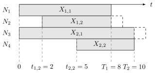
Fig. 1 contains an example that illustrates a scheduling policy and its corresponding completion time and node time. Given two tasks, we launch task 1 at node 1 and 2 at $t_{1,1}=0$ and $t_{1,2}=2$ respectively, and task 2 at node 1 and 2 at $t_{2,1}=0$ and $t_{2,2}=5$ respectively. The running time $X_{1,1}=8$ and $X_{1,2}=7$, and since node 1 finishes the task first at time $t=8$, $T_{1}=8$ and node 2 is terminated before it finishes executing. Similarly, node 3 is terminated as node 4 finishes task 2 first at time $T_{2}=10$. The machine time for each machine is their actual running time, which are 8, 6, 10 and 5 respectively, and hence the total machine time is the sum 29, while completion time is $T=\max\left\{{T_{1},T_{2}}\right\}=10$.

Figure 1: Example illustrating a scheduling policy and its performance, where $\left\{{t_{i,j}}\right\}$ are the starting times for tasks, and $\left\{{X_{i,j}}\right\}$ are the running time for tasks. The machine time is $C=29$ and the completion time is $T=10$.

Cost function

Intuitively, while introducing task replication reduces $T$, it may incur additional resource usage and hence increase $C$. In this work we investigate trade-off between these two quantities. In particular, we define the following cost function:

$$J_{\lambda}(\pi)=\lambda\mathbb{E}\left[{T(\pi)}\right]+(1-\lambda)\mathbb{E}\left[{C(\pi)}\right],$$ (6)

where $0\leq\lambda\leq 1$ reflects the relative importance of completion time.

Remark 1.

$\lambda$ can be used to take cost of completion time and cost of computing resource into account. $\lambda=1$ and $\lambda=0$ correspond to the case of caring about completion time only and machine time only, respectively.

2.4 Optimal and suboptimal policies

The introduction of cost function $J_{\lambda}(\cdot)$ allows us to compare policies directly, and we define optimal and suboptimal policies.

Definition 1 (Optimal and suboptimal policies).

Given $\lambda$, then the corresponding optimal scheduling policy $\pi^{*}$ is

$$\pi^{*}=\operatorname*{arg\,min}_{\pi}J_{\lambda}(\pi).$$

Remark 2.

Note that there may exist policies that are neither optimal nor suboptimal.

However, the search space for optimal policy is non-trivial, as the cost function is not non-convex, and the search space is large, because we can launch any number of machines at any time before $\alpha_{l}$.

For the rest of the paper, we tackle the optimization problem by narrowing down the search space, solving for special yet important cases, and proposing heuristic algorithms.

3 Motivating example

In this section we consider the following example, which shows in certain scenarios, task replication reduces both $\mathbb{E}\left[{T}\right]$ and $\mathbb{E}\left[{C}\right]$, even for a single task!

Let the execution time $X$ satisfies

$$X=\begin{cases}2&\text{w.p. }0.9\\ 7&\text{w.p. }0.1\end{cases}.$$

(a) $P_{T}$ without replication

(b) $P_{T}$ with replication at $t=2$

Figure 2: Execution time distribution

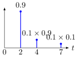
If we launch one task and wait for its completion, then the completion time distribution is illustrated in Fig. 2(a), and

$$T =2\times 0.9+7\times 0.1=2.5$$ (7)

$$C_{\mathrm{loud}} =T=2.5.$$ (8)

If we launch a task at time $t_{1}=0$ and then launch a replicated task at time $t_{2}=2$ if the first one has not finished running by then, we have the completion time distribution in Fig. 2(b), and in this case,

$$T =2\times 0.9+4\times 0.09+7\times 0.01=2.23$$

$$C_{\mathrm{loud}} =2\times 0.9+(4+2)\times 0.09+(7+5)\times 0.01=2.46.$$

As we see here, introducing replication actually reduces both expected cost and expected execution time!

4 Single-task scheduling

In this section we present our results regarding the optimal scheduling for a single task. While this seems simplistic, it is practically useful if we cannot divide a job into multiple parallel tasks. In addition, it is impossible to scheduling multiple tasks optimally if we do not even understand how to schedule a single task optimally.

We postpone all proofs to Section 6.

We first note that in a single-task scheduling scenario, we can represent a scheduling policy by its starting time vectors, i.e.,

$$\pi=\mathbf{t}=[t_{1},t_{2},\ldots,t_{m}],$$

where $t_{j}$ is the time that the task starts on machine $j$.

Remark 3.

Note that the starting time vector $[t_{1},\ldots,t_{m}]$ is equivalent to $[t_{1},t_{2},\ldots,$ $t_{m},\alpha_{l},\ldots,\alpha_{l}]$ as tasks scheduled to start at $\alpha_{l}$ will never be launched. We use the two representations interchangeably in this paper.

The performance metrics, completion time $T$ and cost $C_{\mathrm{loud}}$, can now be expressed as

$$T =\min_{1\leq j\leq m}t_{j}+X_{j},$$ (9)

$$C_{\mathrm{loud}} =\sum_{j=1}^{m}\left|{T-t_{j}}\right|^{+},$$ (10)

where $X_{j}\stackrel{{\scriptstyle~{}{i.i.d.}}}{{\sim}}P_{X}$.

We then show in Theorem 1 that in single-task scheduling, dynamic launching and static launching policies are equivalent in the sense that they achieve the same $\mathbb{E}\left[{C}\right]$-$\mathbb{E}\left[{T}\right]$ tradeoff.

Theorem 1.

For single task scheduling, the static launching policy achieves the same $\mathbb{E}\left[{C}\right]$-$\mathbb{E}\left[{T}\right]$ tradeoff region as the dynamic launching policy.

Remark 4.

The above result does not hold for scheduling multiple tasks in general, as the dynamic launching policy can take different actions depending on if any other tasks are finished.

Therefore, for the single-task scenario, we can focus on the static launching policy without any loss of generality.

4.1 General execution time distribution

Given the machine execution time distribution $P_{X}$ and a starting time vector $\mathbf{t}=[t_{1},\ldots,t_{m}]$, we first show an important property of $\mathbb{E}\left[{T(\mathbf{t})}\right]$ and $\mathbb{E}\left[{C(\mathbf{t})}\right]$ in Theorem 2.

Theorem 2.

$\mathbb{E}\left[{T(\mathbf{t})}\right]$ and $\mathbb{E}\left[{C(\mathbf{t})}\right]$ are piecewise linear functions of $\mathbf{t}$.

A further refinement of Theorem 2 results Theorem 3, which indicates the optimal starting time vector $\mathbf{t}\in[0,\alpha_{l}]^{m}$ is located in a finite set, which is composed by a constrained integer combination of the support of $P_{X}$.

Theorem 3.

The starting time vector $\mathbf{t}=[t_{1},\ldots,t_{m}]$ that minimizes $J_{\lambda}$ satisfies that

$$t^{*}_{j}\in\mathcal{V}_{m},$$ (11)

where $\mathcal{V}_{m}$ is a finite set such that

$$\mathcal{V}_{m}\triangleq\left\{v:v=\sum_{j=1}^{l}\alpha_{j}w_{j},0\leq v\leq\alpha_{l},\sum_{j=1}^{l}\left|w_{j}\right|\leq m,w_{j}\in\mathbb{Z}\right\}.$$ (12)

Theorem 3 directly leads to Section 4.1.

Corollary .

If PMF $P_{X}$ satisfies that $\alpha_{j}=k_{j}\alpha,1\leq j\leq l,k_{j}\in\mathbb{Z^{+}}$, then the optimal starting time vector $\mathbf{t}^{*}$ satisfies

$$t_{j}\in\mathcal{V}_{m}\subset\left\{{0,\alpha,2\alpha,\ldots,\alpha_{l}=k_{m}\alpha}\right\},$$

where $\left|\mathcal{V}_{m}\right|\leq k_{m}+1$.

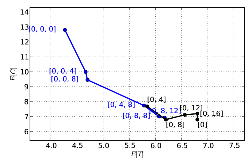
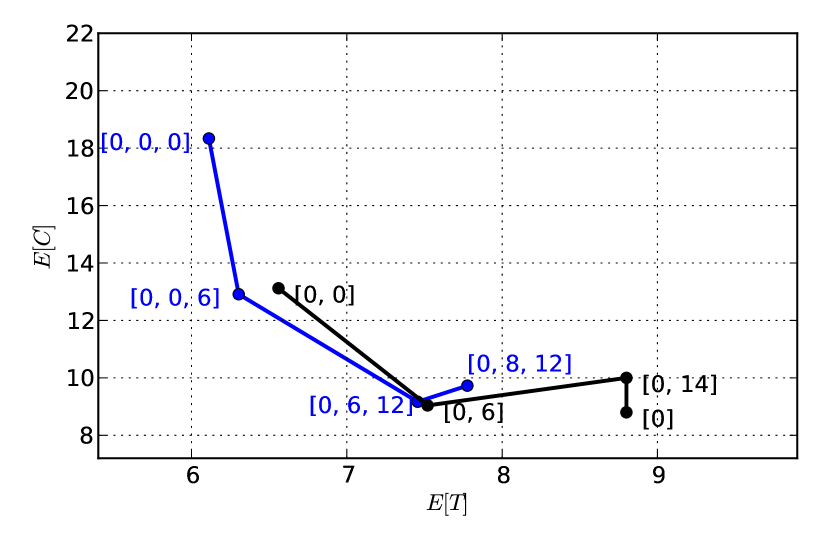
Given Theorem 3, we can calculate the $\mathbb{E}\left[{T}\right]$ and $\mathbb{E}\left[{C}\right]$ for all starting time vectors that satisfy 11, then discard suboptimal ones, leading to the $\mathbb{E}\left[{C}\right]$-$\mathbb{E}\left[{T}\right]$ tradeoff as shown in Fig. 3, which are plotted for the following two execution times:

$$X =\begin{cases}4&\text{ w.p. }0.6\\ 8&\text{ w.p. }0.3\\ 20&\text{ w.p. }0.1\end{cases},$$ (13)

$$X^{\prime} =\begin{cases}6&\text{ w.p. }0.8\\ 20&\text{ w.p. }0.2\end{cases}.$$ (14)

(a) Execution time $X$ in 13

(b) Execution time $X^{\prime}$ in 14

Figure 3: Examples of the $\mathbb{E}\left[{C}\right]$-$\mathbb{E}\left[{T}\right]$ tradeoff with $m=3$ machines. The labels for each point is the corresponding starting time vector, and the region is defined by two piecewise linear segments, which are colored blue and black respectively.

Furthermore, we show that the optimal choice of the $(i+1)$-th element of the starting time vector is dependent on the starting times before it, i.e., $t_{1},t_{2},\ldots,t_{i}$, via Theorem 4. In particular, the optimal value belongs to a set $\mathcal{U}$ that we called corner points and define in Definition 2.

Definition 2 (Corner points).

Given $\mathbf{t}=[t_{1},t_{2},\ldots,t_{i}]$, let

$$\mathcal{U}_{1} \triangleq\left\{{0,\alpha_{1},\ldots,\alpha_{l}}\right\},$$

$$\mathcal{U}_{i+1}(t_{1},\ldots,t_{i}) \triangleq\bigcup_{u\in\mathcal{U}_{i}(t_{1},\ldots,t_{i-1})}\bigg{\{}u+t_{i}-b\alpha_{j}:$$

$$\;\;\qquad 0\leq u+t_{i}-b\alpha_{j}\leq\alpha_{l},$$

$$\;\;\qquad 1\leq j\leq l,b\in\left\{{0,1}\right\}\bigg{\}},\quad i\geq 1,$$

and we called $\mathcal{U}_{i+1}$ the corner points given $\mathbf{t}$.

Theorem 4.

Given $\mathbf{t}=[t_{1},t_{2},\ldots,t_{i}]$ and the corner points $\mathcal{U}_{i+1}(\mathbf{t})$, then the optimal scheduling policy with $i+1$ machines

$$\mathbf{t}^{\prime}=[t_{1},t_{2},\ldots,t_{i},t_{i+1}]$$

satisfies

$$t_{i+1}\in\mathcal{U}_{i+1}.$$

Finally, we have the following simple observation that, again, help to reduce the search space of scheduling policy.

Lemma .

Starting a machine at any time $\alpha_{l}-\alpha_{1}\leq t\leq\alpha_{l}$ is suboptimal.

4.1.1 Heuristic policy search algorithm

While Theorem 3 reduces the search space of the optimal scheduling policy, there could still be exponentially many policies to evaluate. In this section we introduce a heuristic single-task scheduling algorithm in Algorithm 1 that has much lower complexity.

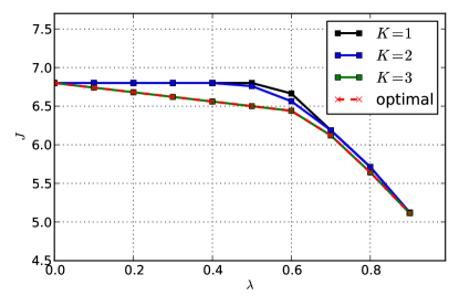
As shown in Algorithm 1, this heuristic algorithm builds the starting time vector $[t_{1},t_{2},\cdots t_{m}]$ iteratively, with the constraint that $t_{i}$’s are in non-decreasing order. Given a starting time vector $[t_{1},\cdots t_{i}]$, this algorithm compares the policies $[t_{1},\cdots t_{i},t_{i+1}]$ where $t_{i+1}$ can be one of first $k$ corner points in $\mathcal{U}(t_{1},\ldots,t_{i})$, and choose the policy $t_{i+1}$ that leads to the minimum cost. As we increase $k$, the algorithm compares a larger space of policies and hence achieves a lower cost as illustrated by the example in Fig. 4, for the execution time defined in 13. The example also demonstrates that a small $k$ may be sufficient to achieve near-optimal cost.

Initialize $t_{1}=0$ and $\mathbf{t}=[t_{1}]$

for $i=2,\ldots m$ do

     $U^{+}(\mathbf{t})\leftarrow$ sorted elements of $\mathcal{U}(\mathbf{t})$ which are $\geq t_{i-1}$

     $\pi_{0}\leftarrow[\mathbf{t},\alpha_{l}]$, policy that keeps the machine unused

     for $j=1,\ldots,k$ do

         $\pi_{j}\leftarrow[\mathbf{t},U^{+}(\mathbf{t})[j]]$

     end for

     $j^{*}\leftarrow\operatorname*{arg\,min}_{j\in{0,1,\cdots k}}J_{\lambda}(\pi_{j})$

     $t_{i}\leftarrow U^{+}(\mathbf{t})[j]$ and $\mathbf{t}\leftarrow[\mathbf{t},t_{i}]$

end for

Algorithm 1 $k$-step heuristic algorithm for single-task scheduling

Figure 4: Comparison between the heuristic search and optimal scheduling policy for execution time in 13.

4.2 Bimodal execution time distribution

While results in Section 4.1 help characterize the $\mathbb{E}\left[{C}\right]$-$\mathbb{E}\left[{T}\right]$ tradeoff and find good scheduling policies, they provide little insight about when and why task replication helps. For this, we analyze the special yet important case of bimodal execution time distribution (cf. 3).

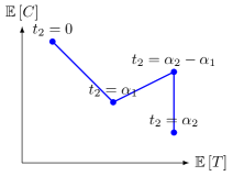
In this section we present results for scheduling one task with two machines, which is the simplest non-trivial example. The scheduling policy can be represented as the vector $\mathbf{t}=[t_{1}=0,t_{2}]$, and we provide a complete characterization of the $\mathbb{E}\left[{C}\right]$-$\mathbb{E}\left[{T}\right]$ tradeoff in Fig. 5, leading to Theorem 5.

Figure 5: The $\mathbb{E}\left[{T}\right]$-$\mathbb{E}\left[{C}\right]$ tradeoff for bimodal execution with two machines, which corresponds to starting time vector $\mathbf{t}=[t_{1}=0,t_{2}]$.

Theorem 5.

Given $P_{X}$ is a bimodal distribution and we have at most two machines, the optimal policy $\mathbf{t}=[t_{1}=0,t_{2}]$ satisfies $t_{2}\in\left\{{0,\alpha_{1},\alpha_{2}}\right\}$.

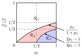
In Theorem 6, we provide further insights by showing the suboptimality (cf. Definition 1) of certain scheduling policies as the execution time distribution $P_{X}$ varies, which is characterized by the ratio of its fast and slow response time, $\alpha_{1}/\alpha_{2}$, and the probability that it finishes at its fast response time, $p_{1}$.

Theorem 6.

Given the bimodal execution time and two machines,

1. $[0,\alpha_{2}-\alpha_{1}]$ is always suboptimal;

2. $[0,\alpha_{1}]$ is suboptimal if $\frac{\alpha_{1}}{\alpha_{2}}>\frac{p_{1}}{1+p_{1}}$;

3. $[0,\alpha_{2}]$ is suboptimal if $\frac{\alpha_{1}}{\alpha_{2}}<\frac{2p_{1}-1}{4p_{1}-1}$;

Given $\lambda$, we can find the optimal policy by comparing the ratio $\frac{1-\lambda}{\lambda}$ to the thresholds,

$$\tau_{1} =\frac{\alpha_{1}p_{1}(3-2p_{1})+\alpha_{2}(1-p_{1})(1-2p_{1})}{(\alpha_{2}-\alpha_{1})(1-p_{1})p_{1}}$$ (15)

$$\tau_{2} =\frac{1+2p_{1}(1-p_{1})}{p_{1}(1-p_{1})}$$ (16)

$$\tau_{3} =\frac{\alpha_{1}(4p_{1}-1)+\alpha_{2}(1-2p_{1})}{\alpha_{2}-2\alpha_{1})p_{1}}$$ (17)

1. If $\frac{\alpha_{1}}{\alpha_{2}}>\frac{p_{1}}{1+p_{1}}$, then policy $[0,\alpha_{2}]$ is optimal if $\frac{1-\lambda}{\lambda}\leq\tau_{1}$, and $[0,0]$ is optimal otherwise.

2. If $\frac{2p_{1}-1}{4p_{1}-1}\leq\frac{\alpha_{1}}{\alpha_{2}}\leq\frac{p_{1}}{1+p_{1}}$, then policy $[0,\alpha_{1}]$ is optimal if $\tau_{3}<\frac{1-\lambda}{\lambda}\leq\tau_{2}$, policy $[0,\alpha_{2}]$ is optimal if $\frac{1-\lambda}{\lambda}\leq\tau_{3}$, and $[0,0]$ is optimal otherwise.

3. If $\frac{\alpha_{1}}{\alpha_{2}}<\frac{2p_{1}-1}{4p_{1}-1}$, then policy $[0,\alpha_{1}]$ is optimal if $\frac{1-\lambda}{\lambda}\leq\tau_{2}$, and $[0,0]$ is optimal otherwise.

Theorem 6 is summarized in Fig. 6.

Figure 6: Bimodal two machine. $\mathcal{R}_{1}$ is the range of parameters that $\mathbf{t}=[0,\alpha_{1}]$ is strictly suboptimal, $\mathcal{R}_{3}$ is the range $\mathbf{t}=[0,\alpha_{2}]$ is strictly suboptimal, which means no task replication is strictly suboptimal.

5 Multi-task scheduling

In this section we investigate the scheduling of multiple tasks. We first show that it is crucial to take the interaction of different tasks into account in Theorem 7, then extend our algorithm in Algorithm 1 for multi-task scheduling. All proofs are postponed to Section 7.

Theorem 7 (Separation is suboptimal).

Given $m$ tasks, applying the optimal one-task scheduling policy for each of them individually is suboptimal.

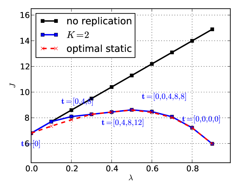
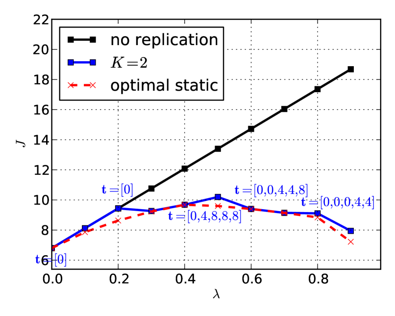
Given the complexity of searching for optimal scheduling policy in the single-task case, we again aim to search for scheduling policy via a heuristic algorithm. In particular, we aim to find a good static policy that takes the interaction among tasks into account. To achieve this, we apply Algorithm 1, but using the cost function for the multi-task case, where $T$ and $C$ are defined in 4 and 5 respectively. This search procedure produces a starting time vector $\mathbf{t}=[t_{1},t_{2},\ldots,t_{m}]$, and at each time $t_{i}$, we launch an additional copy for each of the unfinished task.

Fig. 7 shows an example for the execution time in 13. The scheduling policy with replication reduces $J$, especially when $\lambda$ is large. We also see that as the number of tasks $n$ increases, the cost $J$ increases as the impact of the slowest task gets more severe. Again, introducing replication mitigates this degradation.

Results in Fig. 7 indicate that when $\lambda$ is not too big, it may be beneficial to introduce replication at multiple time instants, as in this case, we are more concerned with cost $C_{\mathrm{loud}}$ and hence introducing replication gradually is preferred. By contrast, when $\lambda$ is close to 1, a good scheduling policy should introduce replication early to cut down completion time as early as possible.

(a) $N=10$ tasks

(b) $N=100$ tasks

Figure 7: Performance of scheduling policy based on heuristic search for execution time in 13. $k$ is the parameter in Algorithm 1. The starting time vector for $k=2$ and $\lambda=0,0.2,0.4,0.6$ and $0.8$ are labeled in the plots.

Remark 5.

Our proposed policy via searching algorithm is static in nature. One may extend it by running the searching algorithm at each time instant. For example, at time $t=0$ we obtain the starting time vector $t^{(0)}$. At time $t=\alpha_{1}$ we can re-run the search algorithm given the number of unfinished tasks and obtain an updated starting time vector $t^{(1)}$, etc.. This policy is dynamic in nature and is likely to achieve better performance than the static policy.

6 Proofs for single task scheduling

In this section we present the detailed analysis for the problem of optimal scheduling for a single task.

6.1 Proofs for Theorem 1

Proof of Theorem 1.

With node completion feedback, at any time $t$, a dynamic launching policy can make launching decision based on whether any running node finishes execution by then, and it is obvious that it should launch new copies only if no node has finished executing the task.

Given a dynamic launching policy $\pi_{\mathrm{DL}}$, we can construct a static policy $\pi_{\mathrm{SL}}$ by letting its starting time vector be the starting time emitted from the dynamic policy under the condition that no machine finishes execution until $\alpha_{l}$. Now we claim $\pi_{\mathrm{DL}}$ and $\pi_{\mathrm{SL}}$ achieves the same $\mathbb{E}\left[{T}\right]$ and $\mathbb{E}\left[{C}\right]$, because it is not difficult to see that for a given realization of machine execution time, both policies will launch and terminate machines at the same time.

6.2 Proofs for Theorem 2 and Theorem 3

In this section we show that the $\mathbb{E}\left[{C}\right]$-$\mathbb{E}\left[{T}\right]$ tradeoff curve is always piecewise linear, with the vertices of the piecewise linear curve corresponding to starting time vector that satisfies certain properties.

We first define the possible finishing time

$$w_{i,j}\triangleq t_{i}+\alpha_{j},1\leq i\leq m,1\leq j\leq l$$

and the set of all possible finishing times

$$\mathcal{W}\triangleq\left\{{w_{i,j},1\leq i\leq m,1\leq j\leq l}\right\}.$$

Let $k=\left|\mathcal{W}\right|$, we denote the sorted version of $\mathcal{W}$ as $\mathbf{w}=[w_{\sigma_{\mathbf{t}}(1)},w_{\sigma_{\mathbf{t}}(2)},\ldots,w_{\sigma_{\mathbf{t}}(k)}]$ such that

$$w_{\sigma_{\mathbf{t}}(1)}\leq w_{\sigma_{\mathbf{t}}(2)}\leq\ldots\leq w_{\sigma_{\mathbf{t}}(k)},$$

where $\sigma_{\mathbf{t}}(k)$ maps the rank of the finishing time $k$ to a tuple $(i_{k},j_{k})$.

Note that

$$T=\min_{1\leq i\leq m}X_{i}+t_{i},$$

and $T\in\mathcal{W}$, we define the event

$$\mathcal{A}_{k_{1},k_{2}}\triangleq\left\{{\min_{1\leq i\leq m,1\leq j\leq l}^{*}\left\{{t_{i}+X_{j}}\right\}=t_{k_{1}}+\alpha_{k_{2}}}\right\},$$

where $\min^{*}$ indicates we always choose the smallest $(k_{1},k_{2})$ (by lexicographic order in $k_{1}$ and $k_{2}$) so that all the events $\left\{{\mathcal{A}_{k_{1},k_{2}},1\leq k_{1}\leq m,1\leq k_{2}\leq l}\right\}$ are disjoint.

Therefore,

$$\mathbb{E}\left[{T}\right] =\sum_{k_{1},k_{2}}\mathbb{E}\left[\left.\!{T}\right|\mathcal{A}_{k_{1},k_{2}}\right]\mathbb{P}\left[{\mathcal{A}_{k_{1},k_{2}}}\right]$$

$$=\sum_{k_{1},k_{2}}(t_{k_{1}}+\alpha_{k_{2}})\mathbb{P}\left[{\mathcal{A}_{k_{1},k_{2}}}\right]$$ (18)

$$\mathbb{E}\left[{C}\right] =\sum_{j=1}^{m}\mathbb{E}\left[{C_{j}}\right]$$

$$=\sum_{j=1}^{m}\sum_{k_{1},k_{2}}\left|{t_{k_{1}}+\alpha_{k_{2}}-t_{j}}\right|^{+}\mathbb{P}\left[{\mathcal{A}_{k_{1},k_{2}}}\right]$$ (19)

To analyze 18 and 19, we first show that the relative ordering of elements in $\mathcal{W}$ determines $\mathbb{P}\left[{\mathcal{A}_{k_{1},k_{2}}}\right]$.

Lemma .

$\mathbb{P}\left[{\mathcal{A}_{k_{1},k_{2}}}\right]$ is independent of $\left\{{\alpha_{j},1\leq l\leq l}\right\}$ given the relative ordering of elements in $\mathcal{W}$, i.e.,

$$\mathbb{P}\left[{\mathcal{A}_{k_{1},k_{2}}}\,\middle|\,{\sigma_{\mathbf{t}}}\right]=f(\sigma_{\mathbf{t}},k_{1},k_{2},p_{1},\ldots,p_{l}),$$ (20)

where $f$ is some function.

Proof.

$\mathcal{A}_{k_{1},k_{2}}$ indicates machine $k_{1}$ is the first machine that finishes execution, and it finishes execution after running for $\alpha_{k_{2}}$. Define $k\triangleq\sigma_{\mathbf{t}}^{-1}(k_{1},k_{2})$, i.e.,

$$t_{k_{1}}+\alpha_{k_{2}}=w_{\sigma_{\mathbf{t}}(k)},$$

then

$$\mathbb{P}\left[{\mathcal{A}_{k_{1},k_{2}}}\,\middle|\,{\sigma_{\mathbf{t}}}\right] =\mathbb{P}\left[{\bigcap_{j\neq k_{1}}\left\{{t_{j}+X_{j}}\right\}>w_{k_{1},k_{2}}}\,\middle|\,{\sigma_{\mathbf{t}}}\right]$$

$$=\prod_{j\neq k_{1}}\mathbb{P}\left[{t_{j}+X_{j}>w_{k_{1},k_{2}}}\,\middle|\,{\sigma_{\mathbf{t}}}\right].$$ (21)

Define

$$\mathcal{P}_{j}\triangleq\left\{p:\sigma_{\mathbf{t}}(i)=(j,p),i>k\right\},$$

which is uniquely determined by $\sigma_{\mathbf{t}}$ and $k$, then for any $i\neq k_{1}$,

$$q_{j}\triangleq\mathbb{P}\left[{t_{j}+X_{j}>w_{k_{1},k_{2}}}\,\middle|\,{\sigma_{\mathbf{t}}}\right]=\sum_{p\in\mathcal{P}_{j}}p,$$ (22)

which is a function of $k$, $\sigma_{t}$ and $\mathbf{p}=[p_{1},p_{2},\ldots,p_{m}]$.

Combing 21 and 22, we have 20.

Proof of Theorem 2.

We prove that there exists finitely many subspaces of $[0,\alpha_{l}]^{m}$ such that in each subspace, $\mathbb{E}\left[{T}\right]$ and $\mathbb{E}\left[{C}\right]$ is a linear function in $\mathbf{t}$, and thus they are piecewise linear in $\mathbf{t}$ on $[0,\alpha_{l}]^{m}$.

Define $\mathcal{B}_{1}(\sigma)\triangleq\left\{\mathbf{t}:\sigma_{\mathbf{t}}=\sigma\right\}$, and $(k_{1},k_{2})=\sigma(k)$, then the set

$$\mathcal{B}_{1}(\sigma) =\left\{\mathbf{t}:t_{1_{1}}+\alpha_{1_{2}}\leq t_{2_{2}}+\alpha_{2_{2}}\leq\ldots\leq t_{k_{1}}+\alpha_{k_{2}}\right\}$$ (23)

is defined by $k-1$ inequalities, and each of this inequality partition the space $[0,\alpha_{l}]^{n}$ into two subspaces. Therefore, $\mathcal{B}_{1}(\sigma)$ is the intersection of $k-1$ connected subspaces, resulting itself being a subspace of $[0,\alpha_{l}]^{m}$. And it is obvious that there are only finitely many such subspaces. Therefore, by Section 6.2 and 18, in each subspace $\mathcal{B}_{1}(\sigma)$, $\mathbb{E}\left[{T}\right]$ is a linear function in $\mathbf{t}$.

Regarding $\mathbb{E}\left[{C}\right]$, we define

$$\mathcal{B}_{2}(\mathbf{b}=[b_{i,j}]_{1\leq i\leq m,1\leq j\leq k},\sigma)\subset\mathcal{B}_{1}(\sigma)$$

$$\triangleq \big{\{}\mathbf{t}:\sigma_{\mathbf{t}}=\sigma,\;\mathbb{I}\left\{{t_{k_{1}}+\alpha_{k_{2}}-t_{i}>0}\right\}\in\left\{{0,1}\right\},$$

$$\qquad(k_{1},k_{2})=\sigma^{-1}(j),1\leq j\leq k\big{\}},$$ (24)

where $\mathbb{I}\left\{{\cdot}\right\}$ is the indicator function. Similar to the argument above, given $\sigma$ and $\mathbf{b}$, $\mathcal{B}_{2}(\mathbf{b},\sigma)$ corresponds to a subspace of $[0,\alpha_{l}]^{m}$ and there are only finitely many such subspaces. By Section 6.2 and 19, in each subspace $\mathcal{B}_{2}(\mathbf{b},\sigma)$, $\mathbb{E}\left[{C}\right]$ is a linear function in $\mathbf{t}$.

Therefore, both $\mathbb{E}\left[{T}\right]$ and $\mathbb{E}\left[{C}\right]$ are piecewise linear functions of $\mathbf{t}$ in $[0,\alpha_{l}]^{m}$.

Proof of Theorem 3.

By Theorem 2 and the fact that $J_{\lambda}$ is a linear combination of $\mathbb{E}\left[{T}\right]$ and $\mathbb{E}\left[{C}\right]$, the optimal $\mathbf{t}^{*}$ that minimizes $J_{\lambda}(\mathbf{t})$ is at the boundaries of two or more subspaces defined in 24.

Then by 23 and 24, it is not hard to see that for some $j_{1},j_{2},j_{3},j_{4}$ and $l_{1},l_{2},l_{3}$, we have

$$t^{*}_{j_{1}}-t^{*}_{j_{2}} =\alpha_{l_{1}}-\alpha_{l_{2}}$$

$$t^{*}_{j_{3}}-t^{*}_{j_{4}} =\alpha_{l_{3}}.$$

Then it is not hard to see that given $m$, $\mathbf{t}=[t_{1},t_{2},\ldots,t_{m}]$, and without loss of generality, let $t_{1}=0$,

$$t^{*}_{i}\in\mathcal{V}_{m},$$

where $\mathcal{V}_{m}$ is defined in 12, i.e.,

$$\mathcal{V}_{m}\triangleq\left\{v:v=\sum_{j=1}^{l}\alpha_{j}w_{j},0\leq v\leq\alpha_{l},\sum_{j=1}^{l}\left|w_{j}\right|\leq m,w_{j}\in\mathbb{Z}\right\}.$$

Note that an element in $\mathcal{V}_{m}$ is uniquely determined by $\mathbf{w}=[w_{1},\ldots,w_{l}]$, and the number of possible $\mathbf{w}$ is

$$2^{l}{{m+l-1}\choose{l-1}}.$$

Therefore,

$$\left|\mathcal{V}_{m}\right|\leq 2^{l}{{m+l-1}\choose{l-1}}\leq[2(m+l-1)]^{l},$$

which is finite given finite $m$ and $l$.

6.3 Proofs related to corner points

Proof of Theorem 4.

Let $U_{i+1}=[u_{1},u_{2},\ldots,u_{k_{i}}]$ be the sorted version of $\mathcal{U}_{i+1}$, then $\mathbb{E}\left[{T(\mathbf{t}^{\prime})}\right]$ and $\mathbb{E}\left[{C(\mathbf{t}^{\prime})}\right]$ are linear in $t_{i+1}$ over the each interval $[u_{j},u_{j+1}],1\leq j\leq k_{i}-1$. Therefore, the optimal $t_{i+1}\in\mathcal{U}_{i+1}$.

6.4 Proof of Section 4.1

Proof of Section 4.1.

Consider a set of $m$ machines on which we run the task according to the policy $\pi=[t_{1},t_{2},\cdots,t_{m}]$. Without loss of generality, we assume $t_{1}=0$. If the starting time of a machine is $\alpha_{l}>t_{j}\geq\alpha_{l}-\alpha_{1}$, the earliest time it can finish execution of the task is $t+\alpha_{1}$. This time is greater than $\alpha_{l}$, the latest time at which the first machine started at time $t_{1}=0$ finishes the task. Thus, starting the machine at time $t_{j}$ only adds to the cost $\mathbb{E}\left[{C}\right]$, without reducing the completion time $\mathbb{E}\left[{T}\right]$. Hence, any starting time $t_{j}\geq\alpha_{l}-\alpha_{1}$ should be replaced by $\alpha_{l}$, which corresponds to not using that machine at all.

6.5 Proof of Theorem 5

Theorem 5 follows directly from the following lemma.

Lemma .

Given $P_{X}$ is a bimodal distribution and we have at most two machines, the expected completion time and total cost satisfies that if $t_{2}+\alpha_{1}<\alpha_{2}$,

$$\mathbb{E}\left[{T}\right] =\alpha_{1}(p_{2}-p_{1})p_{1}+\alpha_{2}p_{2}^{2}+t_{2}p_{1}p_{2},$$

$$\mathbb{E}\left[{C}\right] =\begin{cases}2\mathbb{E}\left[{T}\right]-t_{2}(p_{1}^{2}+p_{2}^{2})&\text{ if }t_{2}<\alpha_{1}\\ 2\mathbb{E}\left[{T}\right]-\alpha_{1}p_{1}-t_{2}p_{2}&\text{ if }t_{2}\geq\alpha_{1}\end{cases};$$

otherwise if $t_{2}+\alpha_{1}\geq\alpha_{2}$,

$$\mathbb{E}\left[{T}\right] =\alpha_{1}p_{1}+\alpha_{2}p_{2}$$

$$\mathbb{E}\left[{T}\right] =2\mathbb{E}\left[{T}\right]-\alpha_{1}p_{1}-t_{2}p_{2}$$

Proof.

By 10 and 9 and calculation.

6.6 Proof of Theorem 6

Proof of Theorem 6.

1. Follows from Section 4.1.

2. If $\frac{\alpha_{1}}{\alpha_{2}}>\frac{1}{2}$ then by Section 4.1 we know that if $[0,\alpha_{1}]$ is suboptimal. Now suppose $\frac{\alpha_{1}}{\alpha_{2}}>\frac{1}{2}$. We know that $\pi_{1}=[0,0]$ and $\pi_{2}=[0,\alpha_{2}]$ are the two extreme ends of the $(\mathbb{E}\left[{C}\right],\mathbb{E}\left[{T}\right])$ trade-off. If the line joining points $(\mathbb{E}\left[{C(\pi_{1})}\right],\mathbb{E}\left[{T(\pi_{1})}\right])$ and $(\mathbb{E}\left[{C(\pi_{2})}\right],\mathbb{E}\left[{T(\pi_{2})}\right])$ lies below $(\mathbb{E}\left[{C(\pi)}\right],\mathbb{E}\left[{T(\pi)}\right])$, then $\pi=[0,\alpha_{1}]$ will be suboptimal. Comparing the slopes of the lines gives the condition $\frac{\alpha_{1}}{\alpha_{2}}>\frac{p_{1}}{1+p_{1}}$.

3. Policy $\pi_{2}=[0,\alpha_{2}]$ is suboptimal if it is dominated by either $\pi=[0,\alpha_{1}]$ or $\pi_{1}=[0,0]$. Both $\pi$ and $\pi_{1}$ give lower expected execution time $\mathbb{E}\left[{T}\right]$ than $[0,\alpha_{2}]$. So if one of them has expected cost $\mathbb{E}\left[{C}\right]$ lower than $[0,\alpha_{2}]$, then it follows that $[0,\alpha_{2}]$ is dominated by that strategy. But the $\mathbb{E}\left[{C}\right]$ with starting time vector $[0,0]$ is always greater than that of $[0,\alpha_{1}]$. Thus, checking if the expected machine $\mathbb{E}\left[{C}\right]$ with $[0,\alpha_{1}]$ is smaller than that for $[0,\alpha_{2}]$, gives the condition $\frac{\alpha_{1}}{\alpha_{2}}<\frac{2p_{1}-1}{4p_{1}-1}$ for suboptimality of $[0,\alpha_{2}]$.

4. , (e), (f) For cost function $J=\lambda\mathbb{E}\left[{T}\right]+(1-\lambda)\mathbb{E}\left[{C}\right]$, the constant cost contour is a line with slope $-\frac{1-\lambda}{\lambda}$. As we increase $J$, the contour line shifts upward until it hits the $(\mathbb{E}\left[{C}\right],\mathbb{E}\left[{T}\right])$ trade-off. The point where it meets the $(\mathbb{E}\left[{C}\right],\mathbb{E}\left[{T}\right])$ trade-off corresponds to the optimal policy. In $\mathcal{R}_{1}$, policy $\pi_{2}=[0,\alpha_{2}]$ is optimal if the slope of the line joining $(\mathbb{E}\left[{C(\pi_{1})}\right],\mathbb{E}\left[{T(\pi_{1})}\right])$ and $(\mathbb{E}\left[{C(\pi_{2})}\right],\mathbb{E}\left[{T(\pi_{2})}\right])$ is less than or equal to $-\frac{1-\lambda}{\lambda}$. We can simplify and show that the slope of the line is $-\tau_{1}$. The result follows from this. Similarly, the slope of the line joining $[0,0]$, $[0,\alpha_{1}]$ is $-\tau_{2}$, and that of the line joining $[0,\alpha_{1}$ and $[0,\alpha_{2}]$ is $-\tau_{3}$. Comparing the slope of the contour, $-\frac{1-\lambda}{\lambda}$ with these slopes gives the conditions of optimality for each of the policies.

7 Proofs for multi-task scheduling

7.1 Proof of Theorem 7

Proof.

We prove the statement by showing an example that a scheduling policy that takes the interaction of task latencies into account (joint policy) is better than a scheduling each task independently (separate policy).

Suppose we have two tasks and $4$ machines. The service time distribution of each machine is bimodal, taking values $\alpha_{1}$ and $\alpha_{2}>\alpha_{1}$ with probability $p_{1}$ and $1-p_{1}$ respectively. Assume $2\alpha_{1}<\alpha_{2}$.

Separate Policy
Consider a policy $\pi_{s}$ where we choose the optimal scheduling policy separately for each task. We can follow the analysis of the bimodal 2-machine case in Section 6.6 as a guideline to choose the optimal policy for each task.

Suppose the policy $[0,\alpha_{2}]$ is optimal for a given cost function. For this to be true, the parameters $\alpha_{1}$, $\alpha_{2}$ and $p_{1}$ need to satisfy,

$$\frac{\alpha_{1}}{\alpha_{2}}>\frac{2p_{1}-1}{4p_{1}-1}$$ (25)

If we run each task on two machines using the policy $[0,\alpha_{2}]$, the expected completion time and cost are,

$$\mathbb{E}\left[{T\left({\pi_{s}}\right)}\right] =p_{1}^{2}\alpha_{1}+(1-p_{1}^{2})\alpha_{2},$$

$$\mathbb{E}\left[{C_{\mathrm{loud}}\left({\pi_{s}}\right)}\right] =2p_{1}^{2}\alpha_{1}+2p_{1}(1-p_{1})(\alpha_{1}+\alpha_{2})+2(1-p_{1}^{2})\alpha_{2}.$$

Joint Policy
Consider a joint policy $\pi_{d}$ where we start with each task according to policy $[0,\alpha_{2}]$. If task 1 (task 2) is served by its machine at time $\alpha_{1}$, we start the execution the task 2 (task 1) on an additional machine at time $\alpha_{1}$.

Using this joint policy the performance metrics are given by

$$\mathbb{E}\left[{T(\pi_{d})}\right] =p_{1}^{2}\alpha_{1}+2p_{1}^{2}(1-p_{1})(2\alpha_{1})+(1-p_{1})^{2}(2p_{1}+1)\alpha_{2},$$

$$\mathbb{E}\left[{C(\pi_{d})}\right] =p_{1}^{2}(2\alpha_{1})+2p_{1}^{2}(1-p_{1})(3\alpha_{1})+(1-p_{1})^{2}(2p_{1}+1)(2\alpha_{2}).$$

We can show that for $2\alpha_{1}<\alpha_{2}$, $\mathbb{E}\left[{T(\pi_{d})}\right]<\mathbb{E}\left[{T(\pi_{s})}\right]$. Now let us find the condition for $\mathbb{E}\left[{C(\pi_{d})}\right]<\mathbb{E}\left[{C(\pi_{s})}\right]$.

$$\mathbb{E}\left[{C(\pi_{d})}\right] <\mathbb{E}\left[{C(\pi_{s})}\right]$$

$$\Rightarrow\qquad\frac{\alpha_{1}}{\alpha_{2}} <\frac{2p_{1}-1}{3p_{1}-1}.$$

Thus, the joint policy gives strictly lower cost $J_{\lambda}=\lambda\mathbb{E}\left[{C}\right]+(1-\lambda)\mathbb{E}\left[{T}\right]$ than the separate policy for any $\lambda$ if

$$\frac{2p_{1}-1}{4p_{1}-1}<\frac{\alpha_{1}}{\alpha_{2}}<\frac{2p_{1}-1}{3p_{1}-1}.$$ (26)

8 Concluding Remarks

In this paper we present the first theoretical analysis of how to effective replicate tasks such that we reduce completion time, with minimum use of extra computing resources.

We show that for certain scenarios, task replication may in fact simultaneously reduce both execution time and resource usage, and in general, it leads to a better response time and computing resource usage trade-off.

Given a discrete approximation to the service time distribution, we characterize the optimal trade-off between execution time and resource usage for the case of scheduling a single task. We show the optimal scheduling policy is in a set of finite size. We also present a low-complexity heuristic algorithm to choose the scheduling policy that is close to optimal. Further, we give insights into extending this analysis to the multi-task case.

Our work answers the questions on when and how task replication helps, and our results provide guidance to scheduling design in data centers, such as the time to launch tasks and the number of time we should replicate it.

This work can be extended in a few directions. First, one can search for better scheduling policies, especially for the multi-task case. Second, in our work we assume the execution time distribution is given or can be estimated, it may be of interest to develop an adaptive scheduling policy that does not require such knowledge. Third, it will be useful to estimate the error due to approximating a continuous execution time distribution by a discrete execution time distribution, either numerically or via simulation. Finally, one can take the effect of queueing of requests at the machines into account and see how that impacts the system performance.

Acknowledgement

We thank Devavrat Shah for helpful discussions.

References

- [1] G. Ananthanarayanan, A. Ghodsi, S. Shenker, and I. Stoica. Effective straggler mitigation: Attack of the clones. NSDI’13, pages 185–198, Berkeley, CA, 2013. USENIX.
- [2] G. Ananthanarayanan, S. Kandula, A. Greenberg, I. Stoica, Y. Lu, B. Saha, and E. Harris. Reining in the outliers in map-reduce clusters using mantri. OSDI’10, pages 1–16, Berkeley, CA, 2010. USENIX.
- [3] S. Boyd, N. Parikh, E. Chu, B. Peleato, and J. Eckstein. Distributed optimization and statistical learning via the alternating direction method of multipliers. Found. Trends Mach. Learn., 3(1):1–122, 2011.
- [4] F. Chang, J. Dean, S. Ghemawat, W. C. Hsieh, D. A. Wallach, M. Burrows, T. Chandra, A. Fikes, and R. E. Gruber. Bigtable: A distributed storage system for structured data. ACM Transactions on Computer Systems (TOCS), 26(2):4, 2008.
- [5] Y. Chen, A. S. Ganapathi, R. Griffith, and R. H. Katz. Analysis and lessons from a publicly available google cluster trace. EECS Department, University of California, Berkeley, Tech. Rep. UCB/EECS-2010-95, 2010.
- [6] W. Cirne, F. Brasileiro, D. Paranhos, Luís Fabrício W. Góes, and W. Voorsluys. On the efficacy, efficiency and emergent behavior of task replication in large distributed systems. Parallel Computing, 33(3):213–234, 2007.
- [7] J. Dean. Achieving rapid response times in large online services. Online at http://research.google.com/people/jeff/latency.html, 2012.
- [8] J. Dean and L. A. Barroso. The tail at scale. Commun. ACM, 56(2):74–80, 2013.
- [9] J. Dean and S. Ghemawat. MapReduce: simplified data processing on large clusters. Commun. ACM, 51(1):107–113, 2008.
- [10] G. D. Ghare and S. T. Leutenegger. Improving speedup and response times by replicating parallel programs on a SNOW. In Job Scheduling Strategies for Parallel Processing, pages 264–287. Springer Berlin Heidelberg, Jan. 2005.
- [11] S. Ghemawat, H. Gobioff, and S. Leung. The google file system. In ACM SIGOPS Operating Systems Review, SOSP ’03, pages 29–43, New York, NY, USA, 2003. ACM.
- [12] G. Joshi, Y. Liu, and E. Soljanin. Coding for fast content download. In Proc. Annu. Allerton Conf. on Commu. Control. & Comput., pages 326–333, Oct. 2012.
- [13] G. Joshi, Y. Liu, and E. Soljanin. On the Delay-Storage trade-off in content download from coded distributed storage systems. arXiv:1305.3945 [cs, math], May 2013.
- [14] W. Neiswanger, C. Wang, and E. Xing. Asymptotically exact, embarrassingly parallel MCMC. arXiv:1311.4780 [cs, stat], Nov. 2013.
- [15] D. Peng and F. Dabek. Large-scale incremental processing using distributed transactions and notifications. OSDI’10, pages 1–15, Berkeley, CA, 2010. USENIX.
- [16] M. L. Pinedo. Scheduling: Theory, Algorithms, and Systems. Springer, Jan. 2012.
- [17] N. B. Shah, K. Lee, and K. Ramchandran. When do redundant requests reduce latency? arXiv:1311.2851 [cs], Nov. 2013.
- [18] A. Vulimiri, P. B. Godfrey, R. Mittal, J. Sherry, S. Ratnasamy, and S. Shenker. Low latency via redundancy. arXiv:1306.3707 [cs], June 2013.
- [19] Wikipedia. Embarrassingly parallel — Wikipedia, the free encyclopedia, Feb. 2013.
- [20] M. Zaharia, A. Konwinski, A. D. Joseph, R. Katz, and I. Stoica. Improving MapReduce performance in heterogeneous environments. OSDI’08, pages 29–42, Berkeley, CA, 2008. USENIX.