SI-HEP-2014-08
QFET-2014-04
Radiative Inflation and Dark Energy RIDEs Again after BICEP2
Following the ground-breaking measurement of the tensor-to-scalar ratio by the BICEP2 collaboration, we perform a statistical analysis of a model that combines Radiative Inflation with Dark Energy (RIDE) based on the potential and compare its predictions to those based on the traditional chaotic inflation potential. We find a best-fit value in the RIDE model of as compared to in the chaotic model, with the spectral index being in both models.
1 Introduction
Recently the BICEP2 collaboration [1] has reported a measurement of the tensor-to-scalar ratio which provides evidence for large-field (e.g. chaotic) inflationary models, as opposed to small-field (e.g. hybrid) inflationary models (for a review of inflationary models see e.g. [2]). BICEP2 provides the first direct measurement of the large scale -mode polarisation power spectrum. This receives a contribution only from tensor perturbations and, therefore, the detection of a non-vanishing -mode polarisation is direct evidence for the presence of tensor perturbations. More indirectly, temperature anisotropies can also potentially give evidence of tensor perturbations. In this way, prior to BICEP2, the Planck collaboration had placed an upper bound assuming no running of the scalar spectral index. The origin of this disagreement could either be some statistical or systematic effect, or perhaps the first evidence for a running spectral index that would relax the Planck limit to [3], which is well compatible with the BICEP2 measurement.
The BICEP2 results [1] have, within a short time, triggered a series of papers on model updates in the light of the new measurement. Among the models investigated are several scenarios of chaotic inflation [4, 5, 6], broken primordial power spectrum models [7], gravity-related scenarios [8, 9, 10, 11, 12, 13, 14, 15, 16], Higgs-related inflation [17, 18, 19, 20, 21, 22, 23], scenarios related to supersymmetry [24, 25, 26, 27], curvaton model [28], or natural inflation [29, 30]. Furthermore, several general analyses of collections of simple models have been presented [31, 32], general statements about the properties of the inflationary potential are available [33, 34, 35, 36] as well as studies of the consistency of the Planck and BICEP2 data sets [37, 38], and a general discussion about what we can learn from the exciting new results [39, 40, 41].
None of the above studied models of inflation is able to simultaneously account for both inflation in the early Universe and the preponderance of Dark Energy in the Universe at the current epoch [42, 43]. Motivated by the desire to account for both phenomena, some time ago we proposed a model of Radiative Inflation and Dark Energy (RIDE) [44]. Earlier attempts [45], based on the “schizon model” [46, 47, 48], were formulated in the framework of chaotic inflation, which was subsequently essentially excluded by WMAP 5-year data [49]. The question we considered was whether the nice feature of such models, namely that they naturally generate a pseudo Nambu-Goldstone boson (PNGB), which receives a potential via gravitational effects [50] and can then be used as quintessence field, could be implemented within a viable model of inflation.
In this note, following the BICEP2 measurement, we revisit the RIDE model [44] based on the idea of a massive complex scalar field whose mass squared is driven negative close to the Planck scale by radiative effects, leading to a potential of the form111This potential belongs to a class of scenarios recently studied in a systematic way in [51]. which may be compared to the traditional chaotic potential.222We emphasise that both RIDE and chaotic inflation share the need to forbid a possible quartic term , or at least suppress it sufficiently. As this cannot be achieved at the level of an effective theory, it is necessary to resort to a concrete model realisation. This fact has already been commented in [44], and an example of such a framework was also presented where the absence of the quartic term was achieved in a supersymmetric context where no -terms arise. We refer the inclined reader to [44] for a more detailed discussion. The potential is invariant under a global symmetry, and the absolute value of the complex field plays the role of the inflaton field which rolls slowly down a simple potential that resembles chaotic inflation for high field values. Similar to chaotic inflation, the RIDE model leads to predictions for inflation which were fully consistent with WMAP 7-year data [52], but potentially threatened later on by Planck [3]. However, unlike the chaotic model, at the end of inflation the inflation field settles at a non-trivial minimum, thereby breaking the global and generating a PNGB which receives a small mass via gravitational effects. The resulting effective potential for the PNGB is of a form which is suitable for a quintessence field. Thus the PNGB can explain the existence of Dark Energy. Here we perform a statistical analysis of the RIDE model and compare its predictions to those of the chaotic inflation model. We find a best-fit value in the RIDE model of as compared to in the chaotic model, with the spectral index being in both models.
2 Review of the RIDE model
The model is based on a complex scalar field
| (1) |
with , whose tree-level potential has a simple quadratic form, . Including radiative corrections, the mass squared can be driven negative at some scale not too far below the Planck scale. The mechanism of radiative symmetry breaking is well-known in the minimal supersymmetric standard model [53], where the Higgs mass squared is driven negative at the TeV scale. Similarly, radiative symmetry breaking can play an important role in different contexts [54, 55], where a mass squared is driven negative at a much higher scale. See also Ref. [56] for a recent treatment of radiative corrections to inflationary potentials. Such a radiatively corrected potential may be parametrised as [54, 55],
| (2) |
This potential, schematically depicted in Fig. 1, generates a vacuum expectation value (VEV) for the real scalar field . The constant is chosen in a way to yield a potential with value at its minimum. This corresponds to having a vanishing cosmological constant at the end of inflation. As will be discussed below, the Dark Energy dominating today’s Universe is then realised through a quintessence field, one of the key features of the RIDE model. Note that we could in principle have chosen a larger value for , too, which would however complicate the quintessence part. Note further that the predictions for inflation are nearly independent of as long as , i.e., the constant is significantly smaller than the value of the potential -folds before the end of inflation.
Interpreting as the inflaton field, inflation can completely take place in a region where . With the -factor in Eq. (2) being well-behaved, feels a potential that is very similar to the one used for quadratic inflation. Therefore, we expect only small differences in the predictions for inflation in the RIDE model compared to chaotic inflation, see Sec. 3.
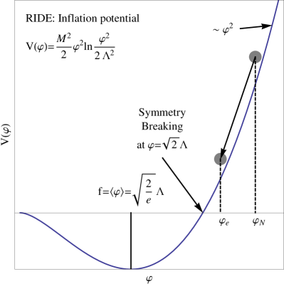
The main advantage of the RIDE model versus a model of inflation lies in the possibility to incorporate a quintessence field to explain Dark Energy. As the minimum of the RIDE potential, Eq. (2), is displaced from , the symmetry gets broken when the inflaton field settles to its VEV. This results in a massless Nambu-Goldstone boson , corresponding to the phase of the complex scalar field . Gravitational effects [45, 50], called gravitational instantons, then generate a potential for which must respect a discrete shift symmetry , with . It is possible to argue that, see [57], the so-obtained potential for the quintessence field takes the form
| (3) |
where denotes the Dark Energy scale, determined from the instanton action via [50, 58, 59, 60] that can easily reproduce the smallness of the observed scale of Dark Energy . As discussed in [44], the dynamics of the inflaton field and the quintessence field separate. Therefore we are practically dealing with single-field potentials, so that the RIDE model is expected to be safe from potentially dangerous corrections due to (iso-)curvature fluctuations that can appear in multi-field inflation models [61].
3 RIDE vs. chaotic inflation
The RIDE potential of Eq. (2) depends on two mass parameters, and . Assuming close to the Planck scale, GeV, we define
| (4) |
where takes a particular value. However it will turn out that the results in what concerns inflation are quite insensitive to values of in the range . In order to relate the parameters of the potential to physical observables such as the scalar spectral index as well as the tensor-to-scalar ratio , it is convenient to define the slow-roll parameters. There are two common versions of these parameters used in the literature, namely the “potential slow-roll parameters” and the “Hubble slow-roll parameters” , which are related as [62]
| (5) |
where the dots indicate higher-order corrections to these relations. It is typically sufficient to consider the first-order relations, so that one can easily convert from one convention to the other. In the following we adopt the potential slow-roll parameters, which in the RIDE model take the form333Note that in [44] we chose to work with the Hubble slow-roll parameters instead.
| (6) | |||||
| (7) | |||||
| (8) |
where and , and the third derivative potential parameter will be relevant for the running of the scalar spectral index. Note that these expressions are independent of the parameter .444Note that should not be confused with the scale of inflation given by . The end of inflation is reached when the Hubble slow-roll parameter . In our numerically calculation of the field value at the end of inflation we make use of the corresponding (approximate) condition . In practice, is always well above . Having determined , we have to find the field value , -folds before the end of inflation. This is achieved by solving
| (9) |
numerically, with being the exponential integral , , and lying within the interval . Using the so-obtained value of (for a fixed value of ), the parameter in Eq. (2) can be directly constrained by the observed scalar perturbations in the Cosmic Microwave Background, as discussed in [44]. One finds where this result is essentially independent of the scale , thanks to the logarithmic dependence of on .
Starting from certain values for and , the two parameters of the potential in Eq. (2), and , are thus fixed. Moreover, the field values at the end of inflation as well as -folds before, , are determined via the procedure discussed above. It is now straightforward to calculate the RIDE predictions for the scalar spectral index as well as the tensor-to-scalar ratio for different values of and using the first order expressions,
| (10) | |||||
| (11) |
The running of the scalar spectral index is only important at second order in the small parameters,
| (12) |
which is one of the reasons for not taking it into account explicitly in our simple analysis (we will comment on the other reason in a second). For chaotic inflation the expressions for the slow-roll parameters and the relation between the field values and the number of -foldings simplify to
| (13) |
Formally, this can be obtained from Eqs. (6,7,9) by dropping all terms involving . Evidently in chaotic inflation.
In our statistical study, we have performed a analysis of the RIDE model and of the similar chaotic inflation model. In order to do this, we have extracted several “data” points from the contour in the -plane from the BICEP2 paper [1] by fitting a tilted ellipse to it. This fit resulted in a “best-fit” point of . Note that this point is not identical to the best-fit point given in Ref. [1], which quotes . This difference simply comes from the fact that the errors in the fitted ellipse are effectively symmetrised (in the basis where the tilt vanishes), but it is numerically not very significant and the resulting error is acceptable in a simplified treatment.
Our simplified fit allows to determine the covariance matrix and to construct a function from it as
| (14) |
The numerical values of the matrix are obtained from the semi-minor and semi-major axes of the fitted ellipse, and , by rotating the diagonal matrix by the angle of the tilt (). Note that we have not taken into account the information on the running in Eq. (14), since we have no way to extract the full covariance matrix from Ref. [1], and thus we cannot know how a change in would affect the other variables. However, if one would nevertheless like to at least approximately take into account the running, one could do this by simply using the corresponding best-fit value and range given in Ref. [1] and add this information to Eq. (14) as penalty term, which results in the total function:
| (15) |
is the function we would then have to minimise. However, we will first focus on of Eq. (14) and postpone a discussion of the contribution from the running to the end of this section.
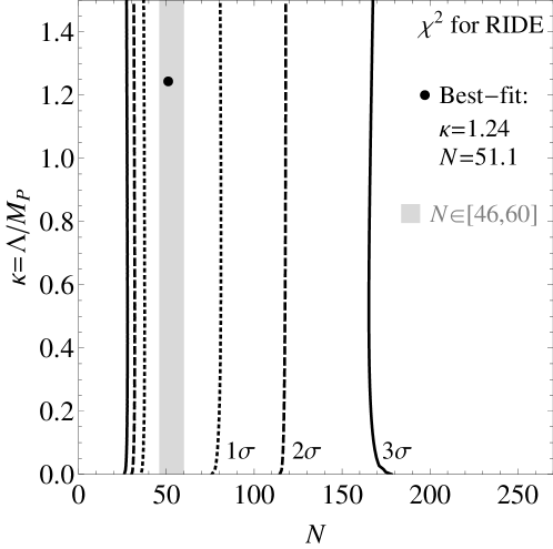
Starting with RIDE, which involves the free parameter , we can calculate the function in the two-parameter plane. The result can be seen in Fig. 2, where we have indicated the (, ) region by the dotted (dashed, solid) lines. The best-fit point turns out to be , with a minimum of which signals a nearly perfect fit. However, as visible in the plot, the function is nearly flat in -direction, so that practically any value of would be allowed [as to be expected since the inflation potential depends only logarithmically on , cf. Eq. (2)]. Note that quintessence imposes a relatively general bound of [44] on this parameter, if too much fine tuning is to be avoided. We will nevertheless display results also for in what follows, in order to make the (weak) dependence of our results on more apparent in the plots. Clearly, the ideal number of -folds clearly is an important parameter, so that we would expect RIDE to fit best in the vicinity of .
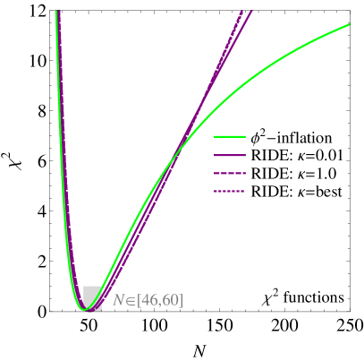
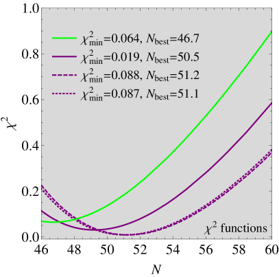
Thus, we can simply take different values of to find a simple comparison between RIDE and inflation, which is displayed in Fig. 3. Glancing at the left panel, it can be seen that all functions look pretty similar, at least up to the range (), while they do visibly differ at (). Indeed when looking closer, see right panel, it is visible that RIDE (for very different values of ) fits marginally better than inflation. When aiming at distinguishing the two models even only at level, one would require an improvement on the knowledge on by more than about an order of magnitude. A distinction at even higher confidence level (such as ) is unlikely to happen within the foreseeable future for . However, it is intriguing that a future CMB polarisation experiment that covers the whole sky and very low instrumental noise might measure with a precision well below , as needed to distinguish RIDE from the model [39] (and surely even more so from [32]). 555Note that, in principle, one could distinguish both models by the running of the scalar spectral index, which is reported to be ( level) [1], since the third derivative of the RIDE potential does not vanish while the one of a potential trivially does. However, in practice both models yield a running which seems too small by about an order of magnitude. We can estimate the running as , which for RIDE is about due to , while . A similar size is obtained for ordinary chaotic inflation.
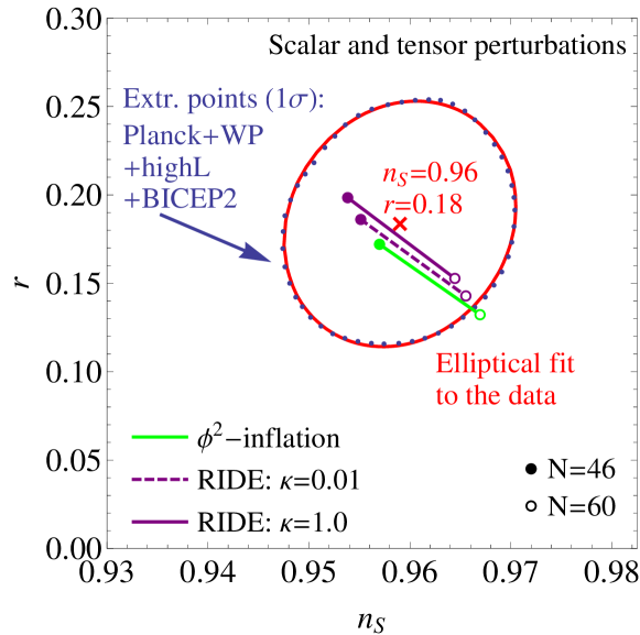
We can display the predictions of both models in the -plane, which further indicates their statistical similarity. This is done in Fig. 4, where also our simple elliptical fit to the extracted “data” points is shown. Indeed, both models give predictions within the region (except for inflation for values of close to 60, but even that does not go far out). The detailed predictions for the best-fit values are:
| Model | |||||
|---|---|---|---|---|---|
| RIDE | |||||
| inflation | — |
Again we can see that the predictions are very similar, if not nearly identical.
Digesting these results, one could question whether any of the two models has any advantage. Indeed there is at least a “theoretical advantage” to the RIDE model: as described in Ref. [44], this model also includes the possibility to explain Dark Energy in terms of a cosine quintessence potential. But, more realistically, it is simply a viable alternative to inflation, and thus one of only a few working examples combining inflation with Dark Energy666It should be noticed that BICEP2 resurrected models as well, though more marginally [32].. If the parameter space shrinks around those two models, both of them would probably have to be viewed as more or less equally good competitors for the true theory behind inflation, since at the moment they are not distinguishable on a statistical basis, as we have shown.
The results on by combining the BICEP2 results with those from Planck temperature anisotropies data, WMAP polarisation, and high experiments as shown in Fig. 4 are obtained allowing for a non-vanishing running of the scalar spectral index and find . As mentioned already, without running BICEP2 results always give , while the Planck+WP+high data lead to an upper bound in tension with BICEP2 results. This seems to strengthen the already existing hint for a non-vanishing value of both from WMAP7 [52] and Planck [3] temperature anisotropies data. The best-fit for the absolute value would be too large compared to the values from single-field inflationary models, including RIDE, predicting . Including errors, the contribution from running to in Eq. (15) gives , quantifying the tension. It should be said, however, that such a tension might be resolved by a better account of foreground contamination or by other systematics. Future data, in particular those expected from Planck on -mode polarisation, will be able to strongly reduce the systematic uncertainties and lead to a much higher statistically significant measurement of the running. Therefore, they will be a crucial test for RIDE, as for all other simple single field inflationary models, that might be (more strongly supported) ruled out if large values of will (not) be confirmed.
4 Conclusions
We have revisited the RIDE model based on radiative symmetry breaking that combines inflation with Dark Energy. We have performed a analysis for the RIDE model parameters and have compared the predictions of RIDE vs. the chaotic inflation model for the spectral index and tensor-to-scalar ratio . The RIDE model gives a slightly better fit to the data than the chaotic inflation model. To be precise we find a best-fit value in the RIDE model of as compared to in the chaotic model, with the spectral index being in both models. In addition, RIDE has the additional advantage that it accounts for the Dark Energy of the universe via the PNGB quintessence field generated at the end of inflation.
Note added
After completion of our work, Refs. [63, 64] appeared where the authors point out how the -mode polarisation signal reported by the BICEP2 collaboration could be partially, if not entirely, due to a foreground contamination effect. In light of this possible effect, much lower values of , even a vanishing one, cannot be currently excluded and new results from Planck or ground based telescopes, such as future Keck Array observations, measuring the signal at different frequencies are needed in order to resolve this ambiguity. As discussed above, our RIDE model fits very well with the BICEP2 determination of , and gives a best fit value of . As can be inferred from Fig. 3, a determination of , at the level of the current Planck upper bound, with an error as for BICEP2, would start to be in tension with the RIDE model, but still compatible. Measuring with a smaller error , as expected from future observations, would, however, strongly disfavour our RIDE model.
Acknowledgments
PDB acknowledges financial support from the NExT/SEPnet Institute and from the STFC Rolling Grant ST/G000557/1. SFK acknowledges support from the STFC Consolidated ST/J000396/1 grant. The work of CL is supported by the Deutsche Forschungsgemeinschaft (DFG) within the Research Unit FOR 1873 (Quark Flavour Physics and Effective Field Theories). AM acknowledges support by a Marie Curie Intra-European Fellowship within the 7th European Community Framework Programme FP7-PEOPLE-2011-IEF, contract PIEF-GA-2011-297557. Finally PDB, SFK, and AM all three acknowledge partial support from the European Union FP7 ITN-INVISIBLES (Marie Curie Actions, PITN-GA-2011-289442).
References
- [1] P. A. R. Ade et al. (BICEP2 Collaboration) (2014), 1403.3985.
- [2] D. H. Lyth and A. Riotto, Phys. Rept. 314, 1 (1999), hep-ph/9807278.
- [3] P. Ade et al. (Planck Collaboration) (2013), 1303.5076.
- [4] K. Harigaya, M. Ibe, K. Schmitz, and T. T. Yanagida (2014), 1403.4536.
- [5] K. Harigaya and T. T. Yanagida (2014), 1403.4729.
- [6] H. M. Lee (2014), 1403.5602.
- [7] D. K. Hazra, A. Shafieloo, G. F. Smoot, and A. A. Starobinsky (2014), 1403.7786.
- [8] P. Channuie (2013), 1312.7122.
- [9] J. Joergensen, F. Sannino, and O. Svendsen (2014), 1403.3289.
- [10] C. Pallis (2014), 1403.5486.
- [11] K. Bamba, R. Myrzakulov, S. D. Odintsov, and L. Sebastiani (2014), 1403.6649.
- [12] F. Bezrukov and D. Gorbunov (2014), 1403.4638.
- [13] S. Ferrara, A. Kehagias, and A. Riotto (2014), 1403.5531.
- [14] T. Kidani and K. Koyama (2014), 1403.6687.
- [15] R. Kallosh, A. Linde, B. Vercnocke, and W. Chemissany (2014), 1403.7189.
- [16] K. Hamaguchi, T. Moroi, and T. Terada (2014), 1403.7521.
- [17] K. Nakayama and F. Takahashi (2014), 1403.4132.
- [18] J. L. Cook, L. M. Krauss, A. J. Long, and S. Sabharwal (2014), 1403.4971.
- [19] C. Germani, Y. Watanabe, and N. Wintergerst (2014), 1403.5766.
- [20] F. Bezrukov and M. Shaposhnikov (2014), 1403.6078.
- [21] R. Costa and H. Nastase (2014), 1403.7157.
- [22] M. Fairbairn, P. Grothaus, and R. Hogan (2014), 1403.7483.
- [23] Y. Hamada, H. Kawai, K.-y. Oda, and S. C. Park (2014), 1403.5043.
- [24] K. Dimopoulos (2014), 1403.4071.
- [25] N. Craig and D. Green (2014), 1403.7193.
- [26] J. Ellis, M. A. G. Garcia, D. V. Nanopoulos, and K. A. Olive (2014), 1403.7518.
- [27] D. H. Lyth (2014), 1403.7323.
- [28] C. T. Byrnes, M. Cortês, and A. R. Liddle (2014), 1403.4591.
- [29] K. Freese and W. H. Kinney (2014), 1403.5277.
- [30] M. Czerny, T. Higaki, and F. Takahashi (2014), 1403.5883.
- [31] T. Kobayashi and O. Seto (2014), 1403.5055.
- [32] N. Okada, V. N. Şenoğuz, and Q. Shafi (2014), 1403.6403.
- [33] S. Choudhury and A. Mazumdar (2014), 1403.5549.
- [34] S. Choudhury and A. Mazumdar, Nucl.Phys. B882, 386 (2014), 1306.4496.
- [35] S. Hotchkiss, A. Mazumdar, and S. Nadathur, JCAP 1202, 008 (2012), 1110.5389.
- [36] Y. Gong (2014), 1403.5716.
- [37] J. McDonald (2014), 1403.6650.
- [38] J.-F. Zhang, Y.-H. Li, and X. Zhang (2014), 1403.7028.
- [39] S. Dodelson (2014), 1403.6310.
- [40] C. Cheng and Q.-G. Huang (2014), 1403.7173.
- [41] C. Cheng and Q.-G. Huang (2014), 1403.5463.
- [42] W. H. Kinney (2009), 0902.1529.
- [43] E. J. Copeland, M. Sami, and S. Tsujikawa, Int. J. Mod. Phys. D15, 1753 (2006), hep-th/0603057.
- [44] P. Di Bari, S. F. King, C. Luhn, A. Merle, and A. Schmidt-May, Phys. Rev. D84, 083524 (2011), 1010.5729.
- [45] R. Rosenfeld and J. A. Frieman, JCAP 0509, 003 (2005), astro-ph/0504191.
- [46] C. T. Hill and G. G. Ross, Nucl. Phys. B311, 253 (1988).
- [47] J. A. Frieman, C. T. Hill, and R. Watkins, Phys. Rev. D46, 1226 (1992).
- [48] J. A. Frieman, C. T. Hill, A. Stebbins, and I. Waga, Phys. Rev. Lett. 75, 2077 (1995), astro-ph/9505060.
- [49] G. Hinshaw et al. (WMAP), Astrophys. J. Suppl. 180, 225 (2009), 0803.0732.
- [50] R. Kallosh, A. D. Linde, D. A. Linde, and L. Susskind, Phys. Rev. D52, 912 (1995), hep-th/9502069.
- [51] J. Martin, C. Ringeval, and V. Vennin (2013), 1303.3787.
- [52] E. Komatsu et al. (2010), 1001.4538.
- [53] L. E. Ibanez and G. G. Ross, Phys. Lett. B110, 215 (1982).
- [54] I. de Medeiros Varzielas and G. G. Ross (2006), hep-ph/0612220.
- [55] R. Howl and S. F. King, Phys. Lett. B687, 355 (2010), 0908.2067.
- [56] K. Enqvist and M. Karciauskas, JCAP 1402, 034 (2014), 1312.5944.
- [57] L. Sorbo, Mod. Phys. Lett. A23, 979 (2008).
- [58] E. Masso and G. Zsembinszki, JCAP 0602, 012 (2006), astro-ph/0602166.
- [59] N. Kaloper and L. Sorbo, Phys. Rev. Lett. 102, 121301 (2009), 0811.1989.
- [60] L. Sorbo Invited talk at the Theory Colloquium, INFN Padua, Italy, Mar. 05, 2009.
- [61] Z. Lalak, D. Langlois, S. Pokorski, and K. Turzynski, JCAP 0707, 014 (2007), 0704.0212.
- [62] A. R. Liddle, P. Parsons, and J. D. Barrow, Phys. Rev. D50, 7222 (1994), astro-ph/9408015.
- [63] M. J. Mortonson and U. Seljak (2014), 1405.5857.
- [64] R. Flauger, J. C. Hill, and D. N. Spergel (2014), 1405.7351.