Residual Symmetries Applied to Neutrino Oscillations at NO$\nu$A and T2K

Abstract

The results previously obtained from the model-independent application of a generalized hidden horizontal $\mathbb{Z}_{2}$ symmetry to the neutrino mass matrix are updated using the latest global fits for the neutrino oscillation parameters. The resulting prediction for the Dirac $CP$ phase $\delta_{D}$ is in agreement with recent results from T2K. The distribution for the Jarlskog invariant $J_{\nu}$ has become sharper and appears to be approaching a particular region. The approximate effects of matter on long baseline neutrino experiments are explored, and it is shown how the weak interactions between the neutrinos and the particles that make up the Earth can help to determine the mass hierarchy. A similar strategy is employed to show how NO$\nu$A and T2K could determine the octant of $\theta_{a}(\equiv\theta_{23})$. Finally, the exact effects of matter are obtained numerically in order to make comparisons with the form of the approximate solutions. From this analysis there emerges some interesting features of the effective mass eigenvalues.

I Introduction

Although there has been significant progress in neutrino physics from oscillation experiments, there remains much work to be done. The reactor angle $\theta_{r}(\equiv\theta_{13})$ has now been measured to greater accuracy than ever before, and the solar angle $\theta_{s}(\equiv\theta_{12})$ has been known for some time now. But, the question of the octant for the atmospheric angle ($\theta_{a}>\frac{\pi}{2}$ or $\theta_{a}<\frac{\pi}{2}$), or whether this angle is maximal ($\theta_{a}=\frac{\pi}{2}$), has yet to be answered. Determination of the Dirac $CP$ phase has been improved. Recent results from T2K exclude at $90\%$ C.L. $\delta_{D}\in[34.2^{\circ},144^{\circ}]$ for normal hierarchy (NH) and $\delta_{D}\in[-180^{\circ},-174.6^{\circ}]\cup[-7.2^{\circ},180^{\circ}]$ for inverted hierarchy (IH) Abe et al. (2014). Finally, the absolute value of the mass squared differences have been carefully measured, but the mass hierarchy is still undetermined (i.e. $m_{3}\gg m_{2}>m_{1}$, or $m_{2}>m_{1}\gg m_{3}$). Each of these questions will be discussed in this work.

From the improvements in recent global analyses Capozzi et al. (2013); Forero et al. (2012); Gonzalez-Garcia et al. (2012) it is possible to make more accurate predictions for the distributions of some of the aforementioned parameters of interest. Specifically, each of the residual symmetries, $\mathbb{Z}_{2}^{s}$ and $\overline{\mathbb{Z}}^{s}_{2}$, can be used to derive a model-independent equation for $\delta_{D}$ (one for each symmetry) Ge et al. (2012); Hanlon et al. (2014). Then using the newly available global fits of the neutrino oscillation parameters in Capozzi et al. (2013), likelihood distributions for $\delta_{D}$, the Jarlskog invariant Jarlskog (1985), and $\theta_{a}$ are obtained.

Using the PMNS mixing matrix, an expression for the probability of a neutrino originally of flavor $\alpha$ to be detected as a neutrino of flavor $\beta$, $P(\nu_{\alpha}\to\nu_{\beta})$, is presented (which is a standard result found in many review papers on neutrino physics Kayser (2004, 2008a, 2008b)). Then, using the approximation from Agarwalla et al. (2013a) it is shown how the earth’s matter affects the neutrino beam in long baseline experiments. This is done by replacing the oscillation parameters with effective values that depend on the energy of the neutrinos, the baseline length, and the density of the matter.

In this paper, a focus is made on the NO$\nu$A and T2K experiments. Both of these experiments measure the appearance of $\nu_{e}$’s ($\overline{\nu}_{e}$’s) from a $\nu_{\mu}$ ($\overline{\nu}_{\mu}$) beam. The probability for this appearance is plotted as a function of energy using the best fits for the oscillation parameters in Capozzi et al. (2013). The effects of matter are taken into account using the average matter density along the baseline for the two experiments. This is justified by the fact that there does not appear to be a significant effect due to the variation of the matter density. A comparison is made for this probability with and without $CP$-violation in an attempt to observe the sensitivity of NO$\nu$A and T2K to measurements of $\delta_{D}$. We have also plotted $P(\nu_{\mu}\to\nu_{e})$ vs. $P(\overline{\nu}_{\mu}\to\overline{\nu}_{e})$ which shows that it may be possible for these experiments to determine the neutrino mass hierarchy for some values of the $CP$ phase as discussed in Patterson (2013); Agarwalla et al. (2013b).

The update of the analysis of Fogli et al. (2012) given in Capozzi et al. (2013) gives closer agreement on $\theta_{a}$ with the other two major global analyses Gonzalez-Garcia et al. (2012); Forero et al. (2012). This shows that $\theta_{a}$ is closer to being maximal than originally believed and only excludes the possibility of it being maximal by about $1\sigma$ for inverted hierarchy. But, it is clear that the analyses do not agree upon which octant is favored. Fortunately, the plots of $P(\nu_{\mu}\to\nu_{e})$ vs. $P(\overline{\nu}_{\mu}\to\overline{\nu}_{e})$ may also serve to determine the octant of $\theta_{a}$ Patterson (2013); Agarwalla et al. (2013b).

This work concludes with a digression into the effective mixing angles and masses in matter. The solar resonance, first described by the MSW effect Wolfenstein (1978); Mikheev and Smirnov (1986); Smirnov (2005), and the atmospheric resonance are readily observed.

II Distribution of $\delta_{D}$, $J_{\nu}$, and $\theta_{a}$

The equations for $\delta_{D}$, in terms of the neutrino mixing angles, based on residual symmetries are given by Ge et al. (2012); Hanlon et al. (2014),

$$\cos\delta_{D}=\frac{(s_{s}^{2}-c_{s}^{2}s_{r}^{2})(s_{a}^{2}-c_{a}^{2})}{4c_{a}s_{a}c_{s}s_{s}s_{r}},$$ (1a)

$$\cos\delta_{D}=\frac{(s_{s}^{2}s_{r}^{2}-c_{s}^{2})(s_{a}^{2}-c_{a}^{2})}{4c_{a}s_{a}c_{s}s_{s}s_{r}},$$ (1b)

for $\mathbb{Z}_{2}^{s}$ and $\overline{\mathbb{Z}}_{2}^{s}$ respectively, where $s_{i}\equiv\sin\theta_{i}$, and $c_{i}\equiv\cos\theta_{i}$. The latest global fits for the neutrino oscillation parameters from Capozzi et al. (2013) are shown in Table 1.

Parameter	Best fit	1$\sigma$ range
$\sin^{2}\theta_{s}/10^{-1}$ (NH or IH)	3.08	2.91-3.25
$\sin^{2}\theta_{r}/10^{-2}$ (NH)	2.34	2.16-2.56
$\sin^{2}\theta_{r}/10^{-2}$ (IH)	2.39	2.18-2.60
$\sin^{2}\theta_{a}/10^{-1}$ (NH)	4.25	3.98-4.54
$\sin^{2}\theta_{a}/10^{-1}$ (IH)	4.37, 5.82*	4.08-4.96 $\oplus$ 5.31-6.10
$\delta_{D}/\pi$ (NH)	1.39	1.12-1.72
$\delta_{D}/\pi$ (IH)	1.35	0.96-1.59
$m_{21}^{2}/10^{-5}eV^{2}$ (NH or IH)	7.54	7.32-7.80
$m_{31}^{2}/10^{-3}eV^{2}$ (NH)	2.48	2.42-2.56
$|m_{31}^{2}|/10^{-3}eV^{2}$ (IH)	2.36	2.29-2.43

Table 1: Global fits for neutrino oscillation parameters from Capozzi et al. (2013). *Represents a local minimum at approximately $0.42\sigma$ for $\chi^{2}$.

From this we can obtain a distribution for $\cos\delta_{D}$ following the procedure in Hanlon et al. (2014); Ge et al. (2012) by using,

$$\frac{dP(\cos\delta_{D})}{d\cos\delta_{D}}=\int\delta^{p}_{D}\mathbb{P}(s_{a}^{2})\mathbb{P}(s_{s}^{2})\mathbb{P}(s_{r}^{2})\mathrm{d}s_{a}^{2}\mathrm{d}s_{s}^{2}\mathrm{d}s_{r}^{2},$$ (2)

where $\delta^{p}_{D}\equiv\delta(\cos{\delta_{D}}-\overline{c}_{D})$, the $\mathbb{P}$’s are proportional to $\exp(-\chi^{2}/2)$, and $\overline{c}_{D}\equiv$ RHS of (1). Because it is preferable to get a distribution with respect to $\delta_{D}$ rather than $\cos\delta_{D}$ we use,

$$\frac{dP(\delta_{D})}{d\delta_{D}}=|s_{D}|\frac{dP(c_{D})}{dc_{D}},$$ (3)

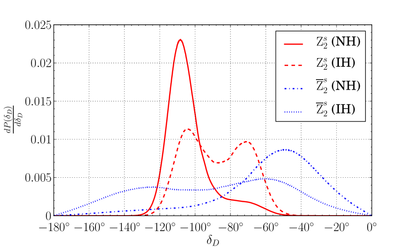
where $c_{D}\equiv\cos\delta_{D}$ and $s_{D}\equiv\sin\delta_{D}$. Since this is a numerical integral, the delta function cannot be used as it is normally defined (unless integrated out of the equation prior to the numerical calculation). The integral was evaluated using a Monte Carlo algorithm and the results are shown in Fig. 1(a). The domain of $\delta_{D}$ in (3) is $[-180^{\circ},0^{\circ}]$, but the distributions in Fig. 1(a) can be reflected about $\delta_{D}=0^{\circ}$ to account for the full interval $[-180^{\circ},180^{\circ}]$. Therefore, these distributions have been normalized to $\frac{1}{2}$ over the domain shown in the figures. This means that each of the residual symmetries will have two peak predictions for the $CP$ phase (equidistant from $0^{\circ}$). The IH $\chi^{2}$ curve for $\theta_{a}$ in Capozzi et al. (2013) is closer to being symmetric about $\sin^{2}\theta_{a}=0.5$. This is very prevalent in the results shown in Fig. 1(a) given that the IH plots are close to being symmetric about $\delta_{D}=-90^{\circ}$. But, since the NH global fit favors the lower octant for $\theta_{a}$ by at least $2\sigma$ Capozzi et al. (2013) the predicted distributions for NH tend to prefer one side of $\delta_{D}=-90^{\circ}$. But in both cases the results for $\mathbb{Z}^{s}_{2}$ are in agreement with the best fit value of $\delta_{D}=-90^{\circ}$ from T2K’s latest results Abe et al. (2014).

The same method is applied to the Jarlskog invariant $J_{\nu}\equiv c_{a}s_{a}c_{s}s_{s}c_{r}^{2}s_{r}s_{D}$ Jarlskog (1985), that is,

$$\frac{dP(J_{\nu})}{dJ_{\nu}}=\int\delta^{p}_{J_{\nu}}\mathbb{P}(s_{a}^{2})\mathbb{P}(s_{s}^{2})\mathbb{P}(s_{r}^{2})\mathrm{d}s_{a}^{2}\mathrm{d}s_{s}^{2}\mathrm{d}s_{r}^{2},$$ (4)

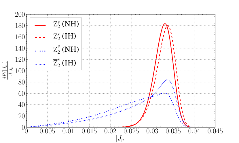
with, $\delta^{p}_{J_{\nu}}\equiv\delta(J_{\nu}-c_{a}s_{a}c_{s}s_{s}c_{r}^{2}s_{r}s_{D})$. This distribution is shown in Fig. 1(b). When calculating these distributions, $\delta_{D}$ is taken to be in the interval $[0,180^{\circ}]$ and is even about the vertical axis to extend $\delta_{D}$ to include $[-180^{\circ},0^{\circ}]$. To account for this, the figures are labeled for the distribution of $|J_{\nu}|$, and they can therefore be normalized to one. As compared with our previous results in Hanlon et al. (2014), $\overline{\mathbb{Z}}^{s}_{2}$ is beginning to favor the region that $\mathbb{Z}^{s}_{2}$ prefers. Also, the region predicted by $\mathbb{Z}^{s}_{2}$ has become slightly narrower and it now excludes $|J_{\nu}|<0.024$.

Finally, this method is again applied similarly to $\theta_{a}$ by first using (1) to solve for $\tan 2\theta_{a}$,

$$\tan 2\theta_{a}=\frac{c_{s}^{2}s_{r}^{2}-s_{s}^{2}}{2c_{s}s_{s}s_{r}\cos\delta_{D}},$$ (5a)

$$\tan 2\theta_{a}=\frac{c_{s}^{2}-s_{s}^{2}s_{r}^{2}}{2c_{s}s_{s}s_{r}\cos\delta_{D}},$$ (5b)

for $\mathbb{Z}_{2}^{s}$ and $\overline{\mathbb{Z}}_{2}^{s}$ respectively. Then we have,

$$\frac{dP(\tan 2\theta_{a})}{d\tan 2\theta_{a}}=\int\delta^{p}_{\theta_{a}}\mathbb{P}(s_{s}^{2})\mathbb{P}(s_{r}^{2})\mathbb{P}(\delta_{D})\mathrm{d}s_{s}^{2}\mathrm{d}s_{r}^{2}\mathrm{d}\delta_{D},$$ (6)

with $\delta^{p}_{\theta_{a}}\equiv\delta(\tan 2\theta_{a}-\overline{t}_{\theta_{a}})$, where $\overline{t}_{\theta_{a}}\equiv$ RHS of (5). To get a distribution for $\theta_{a}$ we use,

$$\frac{dP(\theta_{a})}{d\theta_{a}}=2\sec^{2}(2\theta_{a})\frac{dP(\tan 2\theta_{a})}{d\tan 2\theta_{a}}.$$ (7)

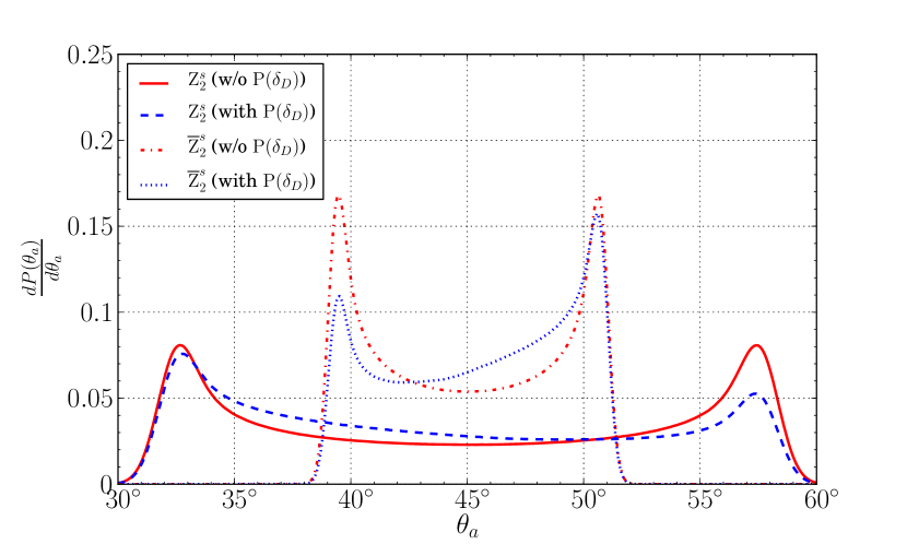
The distribution is shown in Fig. 1(c), where plots are made with and without using the prior on $\delta_{D}$ from Capozzi et al. (2013). When no prior on $\delta_{D}$ is used, $\mathbb{P}(\delta_{D})$ becomes evenly distributed in $[0,2\pi)$. As previously discussed in Hanlon et al. (2014), $\theta_{a}$ is symmetric about $\theta_{a}=45^{\circ}$ when there is no prior on $\delta_{D}$. In addition, the distributions using the prior on $\delta_{D}$ have also become more symmetric, as a result of the $\chi^{2}$ for $\cos\delta_{D}$ also having become more symmetric about zero.

(a)

(b)

(c)

Figure 1: Predicted distributions for (a) $\delta_{D}$, (b) $J_{\nu}$, and (c) $\theta_{a}$ (NH) using the global analysis in Capozzi et al. (2013).

III $\nu_{\mu}$ to $\nu_{e}$ oscillation

Now that we have a distribution for all the neutrino oscillation parameters, an attempt can be made to predict the results of an experiment measuring the number of $\nu_{\mu}$’s that oscillate into $\nu_{e}$’s over some distance. First, the expression for this probability, $P(\nu_{\mu}\to\nu_{e})$, must be found. Denoting the weak eigenstates of the neutrino by $\mid\nu_{\alpha}\rangle$, and the neutrino mass eigenstates by $\mid\nu_{i}\rangle$, then

$$(U_{PMNS})_{\alpha j}\equiv\langle\nu_{\alpha}\mid\nu_{j}\rangle,$$ (8)

defines the PMNS mixing matrix, $U_{PMNS}$. The standard parametrization is given by Agarwalla et al. (2013a),

$$U_{PMNS}=U\mathcal{P},$$ (9)

where

$$U=\begin{pmatrix}c_{s}c_{r}&s_{s}c_{r}&s_{r}e^{-i\delta_{D}}\\ -s_{s}c_{a}-c_{s}s_{a}s_{r}e^{i\delta_{D}}&c_{s}c_{a}-s_{s}s_{a}s_{r}e^{i\delta_{D}}&s_{a}c_{r}\\ s_{s}s_{a}-c_{s}c_{a}s_{r}e^{i\delta_{D}}&-c_{s}s_{a}-s_{s}c_{a}s_{r}e^{i\delta_{D}}&c_{a}c_{r}\end{pmatrix},$$ (10)

$$\mathcal{P}=diag(1,e^{i\alpha_{21}/2},e^{i\alpha_{31}/2}).$$ (11)

From Kayser (2004),

$$Amp(\nu_{\alpha}\to\nu_{\beta})=\sum_{i}U^{*}_{\alpha i}e^{-im_{i}^{2}\frac{L}{2E}}U_{\beta i},$$ (12)

which leads to,

$$P\big{(}\overset{(-)}{\nu_{\alpha}}\to\overset{(-)}{\nu_{\beta}}\big{)}=\delta_{\alpha\beta}-4\sum_{i>j}\mathfrak{R}(U^{*}_{\alpha i}U_{\beta i}U_{\alpha j}U^{*}_{\beta j})\sin^{2}\Big{(}\Delta m^{2}_{ij}\frac{L}{4E}\Big{)}\\ \stackrel{{\scriptstyle+}}{{\left(-\right)}}2\sum_{i>j}\mathfrak{I}(U^{*}_{\alpha i}U_{\beta i}U_{\alpha j}U^{*}_{\beta j})\sin\Big{(}\Delta m^{2}_{ij}\frac{L}{2E}\Big{)}$$ (13)

where $\Delta m^{2}_{ij}\equiv m^{2}_{i}-m^{2}_{j}$, $m_{i}$ is the $i$th mass eigenvalue, $L$ is the distance propagated by the neutrino, and $E$ is the energy of the neutrino. Notice that this probability does not depend on the Majorana phases, and therefore a discussion on these phases will not be pursued here.

Making the following definition Agarwalla et al. (2013a),

$$\Delta_{ij}\equiv\frac{\Delta m^{2}_{ij}}{2E}L,$$ (14)

and noting that, $\Delta_{32}=\Delta_{31}-\Delta_{21}$, then

$$P\big{(}\overset{(-)}{\nu_{\mu}}\to\overset{(-)}{\nu_{e}}\big{)}=4s_{s}^{2}c_{r}^{2}\big{(}s_{s}^{2}s_{r}^{2}s_{a}^{2}+c_{s}^{2}c_{a}^{2}-2c_{s}c_{a}s_{s}s_{r}s_{a}c_{D}\big{)}\\ \times\sin^{2}\Big{(}\frac{\Delta_{21}}{2}\Big{)}+4s_{r}^{2}s_{a}^{2}c_{r}^{2}\sin^{2}\Big{(}\frac{\Delta_{31}}{2}\Big{)}+2s_{s}s_{r}c_{r}^{2}s_{a}\big{(}c_{s}c_{a}c_{D}-\\ s_{s}s_{r}s_{a}\big{)}\Big{[}4\sin^{2}\Big{(}\frac{\Delta_{21}}{2}\Big{)}\sin^{2}\Big{(}\frac{\Delta_{31}}{2}\Big{)}+\sin\big{(}\Delta_{21}\big{)}\sin\big{(}\Delta_{31}\big{)}\Big{]}\\ \overset{+}{(-)}4J_{\nu}\Big{[}\sin^{2}\Big{(}\frac{\Delta_{21}}{2}\Big{)}\sin\big{(}\Delta_{31}\big{)}-\sin^{2}\Big{(}\frac{\Delta_{31}}{2}\Big{)}\sin\big{(}\Delta_{21}\big{)}\Big{]}.$$ (15)

The last term includes the Jarlskog invariant Jarlskog (1985) defined above.

III.1 Matter Effects

As electron neutrinos propagate through the earth, they can interact with electrons via $W$-exchange. In addition, all three neutrino flavors can interact with electrons, protons, or neutrons via $Z$-exchange. Assuming electrically neutral matter, the $Z$-exchange between the neutrinos and protons will cancel exactly with the $Z$-exchange between the neutrinos and electrons Kayser (2004). The contribution from $Z$-exchange can be dropped, because it only adds a multiple of the identity matrix to the Hamiltonian Agarwalla et al. (2013a). Then, under the assumption that $E\ll M_{W}$, the effect of $W$-exchange can be accounted for by modifying the Hamiltonian for neutrinos Kimura et al. (2002a),

$$H=\frac{1}{2E}U\begin{pmatrix}0&0&0\\ 0&\Delta m^{2}_{21}&0\\ 0&0&\Delta m^{2}_{31}\end{pmatrix}U^{\dagger}+\frac{1}{2E}\begin{pmatrix}a&0&0\\ 0&0&0\\ 0&0&0\end{pmatrix},$$ (16)

where $a\equiv 2\sqrt{2}G_{F}N_{e}E$, and $N_{e}$ is the density of electrons. For anti-neutrinos, the Hamiltonian is simply the complex conjugate of (16) with $a\to-a$.

One way to proceed is to diagonalize the Hamiltonian exactly, which has been done analytically Zaglauer and Schwarzer (1988); Kimura et al. (2002a, b). However, this doesn’t give much physical insight into the effects of matter on neutrino oscillations. Approximations in which the mixing angles and mass eigenvalues are replaced by effective values don’t modify any of the equations, and therefore it becomes clear how matter affects neutrinos. A number of approximation schemes have been developed Arafune et al. (1997); Freund (2001); Peres and Smirnov (2004); Akhmedov et al. (2004a, b); Akhmedov and Niro (2008); Cervera et al. (2000). One of the most commonly used of these are the equations derived in Cervera et al. (2000). But, due to the large value of $\theta_{r}$ measured at Daya Bay Dwyer (2013), the approximation in Cervera et al. (2000) begins to fail as is shown in Agarwalla et al. (2013a). In the approximation that is used here, the form of (15) can be used with the following modifications Agarwalla et al. (2013a):

$$\hskip 60.0pt\theta_{s}\to\theta^{\prime}_{s},\hskip 20.0pt\theta_{r}\to\theta^{\prime}_{r},\\ \Delta m^{2}_{21}\to\lambda_{2}-\lambda_{1},\hskip 20.0pt\Delta m^{2}_{31}\to\lambda_{3}-\lambda_{1},\hskip 10.0pt$$ (17)

with,

$$\tan(2\theta^{\prime}_{s})=\frac{(\Delta m^{2}_{21}/c^{2}_{r})\sin(2\theta_{s})}{(\Delta m^{2}_{21}/c^{2}_{r})\cos(2\theta_{s})-a},$$ (18a)

$$\tan(2\theta^{\prime}_{r})=\frac{(\Delta m^{2}_{31}-\Delta m^{2}_{21}s^{2}_{s})\sin(2\theta_{r})}{(\Delta m^{2}_{31}-\Delta m^{2}_{21}s^{2}_{s})\cos(2\theta_{r})-a},$$ (18b)

$$\lambda^{\prime}_{\pm}\equiv\frac{(\Delta m^{2}_{21}+ac^{2}_{r})\pm\sqrt{(\Delta m^{2}_{21}-ac^{2}_{r})^{2}+4ac^{2}_{r}s^{2}_{s}\Delta m^{2}_{21}}}{2},$$ (18c)

$$\lambda^{\prime\prime}_{\pm}\equiv\frac{\lambda+(\Delta m^{2}_{31}+as^{2}_{r})\pm\sqrt{[\lambda-(\Delta m^{2}_{31}+as^{2}_{r})]^{2}+4a^{2}sc^{2}_{r}s^{2}_{r}}}{2}.$$ (18d)

Where, for neutrinos let,

$$\hskip 40.0pt\lambda\equiv\lambda^{\prime}_{+},\hskip 20.0pts\equiv s^{\prime 2}_{s},\hskip 20.0pt\lambda_{1}\approx\lambda^{{}^{\prime}}_{-},\\ \lambda_{2}\approx\lambda^{{}^{\prime\prime}}_{\mp},\hskip 25.0pt\lambda_{3}\approx\lambda^{{}^{\prime\prime}}_{\pm},\hskip 45.0pt$$ (19)

and for anti-neutrinos let,

$$\hskip 30.0pt\lambda\equiv\lambda^{\prime}_{-},\hskip 20.0pts\equiv c^{\prime 2}_{s},\hskip 20.0pta\to-a,\\ \lambda_{1}\approx\lambda^{{}^{\prime\prime}}_{\mp},\hskip 20.0pt\lambda_{2}\approx\lambda^{{}^{\prime}}_{+},\hskip 20.0pt\lambda_{3}\approx\lambda^{{}^{\prime\prime}}_{\pm},\hskip 25.0pt$$ (20)

with the upper sign for normal hierarchy and the lower sign for inverted hierarchy.

It’s helpful to show $a$ and $\Delta_{ij}$ in conventional units. Following Agarwalla et al. (2013a),

$$\Delta_{ij}=2.534\bigg{(}\frac{\Delta m^{2}_{ij}}{[eV^{2}]}\bigg{)}\bigg{(}\frac{[GeV]}{E}\bigg{)}\bigg{(}\frac{L}{[km]}\bigg{)}$$ (21a)

$$a=(7.63\times 10^{-5}[eV^{2}])\bigg{(}\frac{\rho}{[g/cm^{3}]}\bigg{)}\bigg{(}\frac{E}{[GeV]}\bigg{)}.$$ (21b)

III.2 NO$\nu$A and T2K

NO$\nu$A is a long-baseline neutrino oscillation experiment located in northern Minnesota. It has a baseline length of $810$ $km$, has an average matter density of $2.8$ $g/cm^{3}$ along this baseline, and a peak neutrino energy around $2$ $GeV$ Patterson (2013). T2K is another neutrino oscillation experiment with similar goals to that of NO$\nu$A. Its baseline length is $295$ $km$, has an average matter density of $2.6$ $g/cm^{3}$, and the neutrino beam energy peaks around $0.6$ $GeV$ Hagiwara et al. (2011).

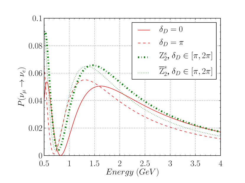
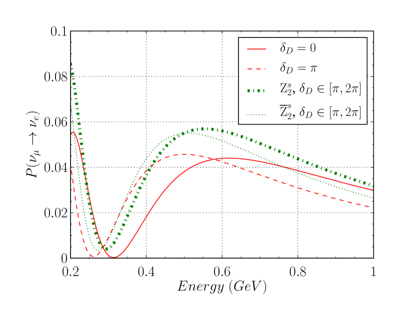
With the use of the effective mixing angles derived in the previous section, the probability of the appearance of a $\nu_{e}$ ($\overline{\nu}_{e}$) from a $\nu_{\mu}$ ($\overline{\nu}_{\mu}$) beam can be determined for any matter density. Using the length and matter density for the two experiments in question, plots of these probabilities are shown in Fig. 3 as a function of energy.

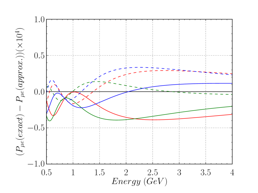
It’s not entirely apparent that the approximation Agarwalla et al. (2013a) is valid for different values of the $CP$ phase or the vacuum mixing angles, therefore a comparison is made between this approximation and the exact results in the Appendix. In this comparison, the exact results are found by numerically diagonalizing the Hamiltonian. As it turns out, the approximation is very good for the energies and densities considered here.

(a)

(a)

Figure 3: $P(\nu_{\mu}\to\nu_{e})$ as a function of energy at (a) NO$\nu$A and (b) T2K, using the best fits from Capozzi et al. (2013) with normal hierarchy.

IV Determination of the Mass Hierarchy and the Octant of $\theta_{a}$

As has been mentioned previously, a major goal of neutrino oscillation experiments is to determine the mass hierarchy. If $CP$ was a good symmetry, then there would be no observable difference between $P(\nu_{\mu}\to\nu_{e})$ and $P(\overline{\nu}_{\mu}\to\overline{\nu}_{e})$ when the neutrinos are propagating through a vacuum. However, interestingly enough, the matter effects discussed above emulate the effects of $CP$-violation. Therefore, there is an observable difference between $P(\nu_{\mu}\to\nu_{e})$ and $P(\overline{\nu}_{\mu}\to\overline{\nu}_{e})$ even if $CP$ is a good symmetry. Without the effects of matter the difference between oscillation probabilities for normal hierarchy versus inverted hierarchy is minimal. Thus it is because of the interactions with matter that allow for a discernible difference between normal and inverted hierarchy.

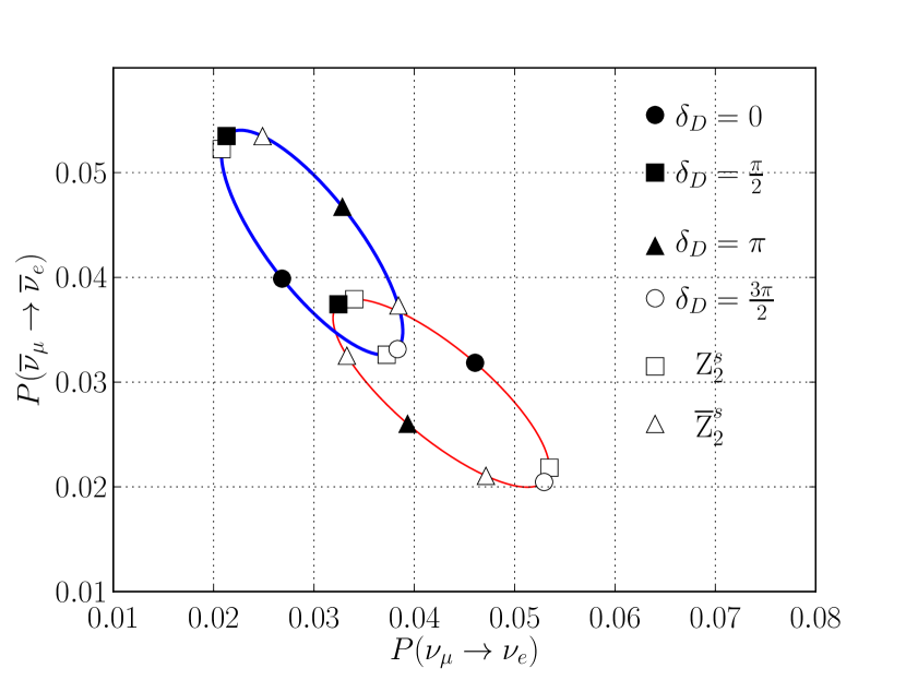
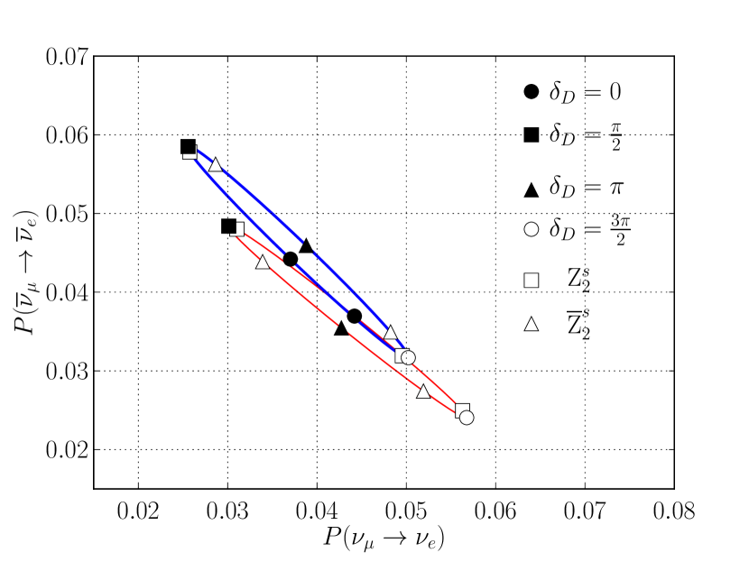
It is possible that actual $CP$-violation is substantially cancelled by this matter induced $CP$-violation. This would be very unfortunate, because it would make the determination of the $CP$ phase more difficult than expected. A plot for $P(\nu_{\mu}\to\nu_{e})$ vs. $P(\overline{\nu}_{\mu}\to\overline{\nu}_{e})$ is shown in Fig. 5 for NO$\nu$A and T2K using the best fits from Capozzi et al. (2013). It can be seen that there are many values of the $CP$ phase that will allow NO$\nu$A to make a serious determination of the true mass hierarchy. This will occur if $\delta_{D}\in[\pi,2\pi]$ with NH being the true hierarchy, or $\delta_{D}\in[0,\pi]$ with IH being the true hierarchy. And since T2K has excluded most of $\delta_{D}\in[0,\pi]$ at $90\%$ C.L. Abe et al. (2014), hopefully the true mass hierarchy is normal. From Fig. 5(a) it appears that T2K will not be able to determine the mass hierarchy in this manner.

In addition, it may also be possible to determine the

(a)

(a)

Figure 5: Plot of $P(\nu_{\mu}\to\nu_{e})$ vs. $P(\overline{\nu}_{\mu}\to\overline{\nu}_{e})$ to show the sensitivity of (a) NO$\nu$A (b) T2K to determining the mass hierarchy assuming $\theta_{a}<\frac{\pi}{2}$. The red ellipse (lower right corner) corresponds to NH, and the blue ellipse (upper left corner) corresponds to IH.

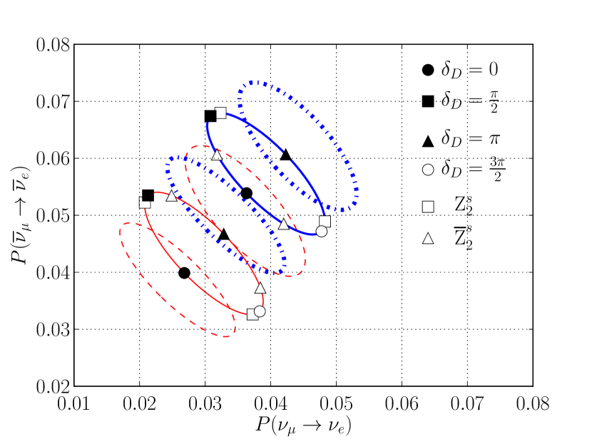
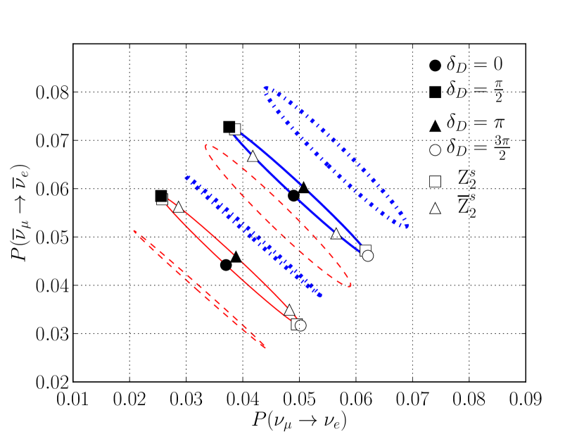
octant of $\theta_{a}$ from similar plots. These are shown in Fig. 7. It appears that every value of the $CP$ phase could at least give some indication of the true octant of $\theta_{a}$, but the best values would be $\delta_{D}=0$ for the lower octant and $\delta_{D}=\pi$ for the higher octant.

The ellipses were created by using (15) with the matter effect modifications of (17). for all possible values of $\delta_{D}$ (i.e. $\delta_{D}$ $\in$ $[0,2\pi]$). The $\Box$ and the $\bigtriangleup$ symbols correspond to the predicted values for $\delta_{D}$, based on $\mathbb{Z}^{s}_{2}$ and $\overline{\mathbb{Z}}^{s}_{2}$, respectively. The predicted values are determined by using the best fits from Capozzi et al. (2013) in (1).

(a)

(a)

Figure 7: Plot of $P(\nu_{\mu}\to\nu_{e})$ vs. $P(\overline{\nu}_{\mu}\to\overline{\nu}_{e})$ to show the sensitivity of (a) NO$\nu$A (b) T2K to determining the octant of $\theta_{a}$ assuming inverted hierarchy. The red ellipses (lower left corner) correspond to $\theta_{a}<\frac{\pi}{4}$, while the blue ellipses (upper right corner) correspond to $\theta_{a}>\frac{\pi}{4}$. The dashed ellipses correspond to the $\pm 1\sigma$ values.

V Effective Masses and Mixing Angles in Matter

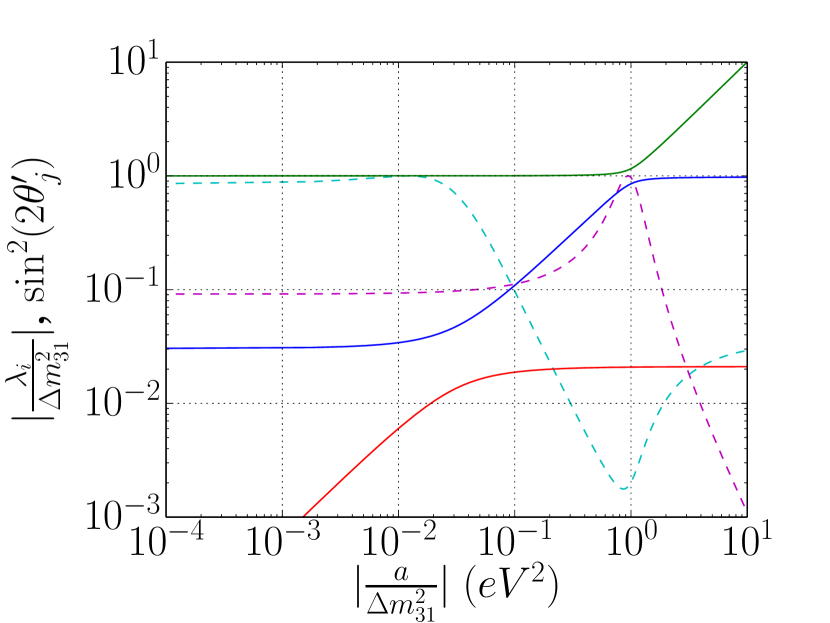
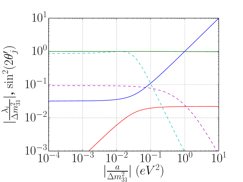
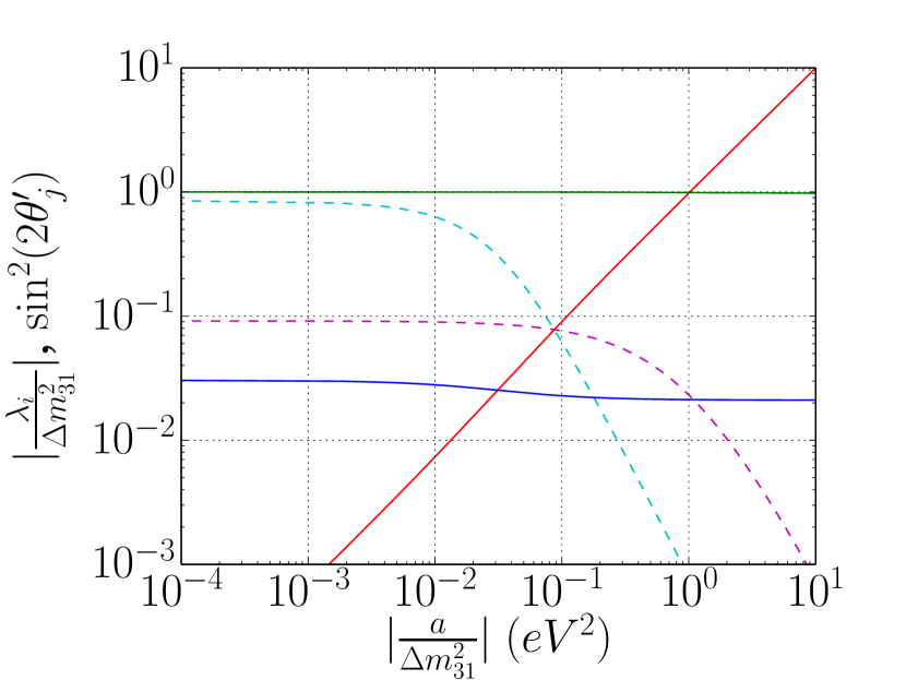
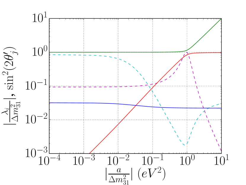
The values of the effective mixing angles are plotted in Fig. 9, and the mass eigenvalues in Fig. 13, as functions of energy using the matter density for the NO$\nu$A experiment. The plots for T2K are excluded here, because they don’t differ much from the ones for NO$\nu$A. Also, these particular plots consider $\delta_{D}=0$, because the results depend very little on the $CP$ phase. These have

(a)

(a)

Figure 9: Plots of the effective mixing angles as a function of energy using data from Capozzi et al. (2013). For (a) NO$\nu$A and neutrinos, (b) NO$\nu$A and anti-neutrinos. Key: red $=\theta^{\prime}_{s}$, blue $=\theta^{\prime}_{a}$, and green $=\theta^{\prime}_{r}$. The solid lines are for normal hierarchy, and the dashed lines are for inverted hierarchy. On the plots where the dashed line is not visible, it’s because the solid line is on top of it.

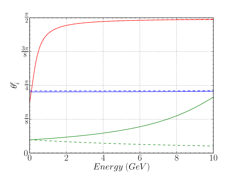
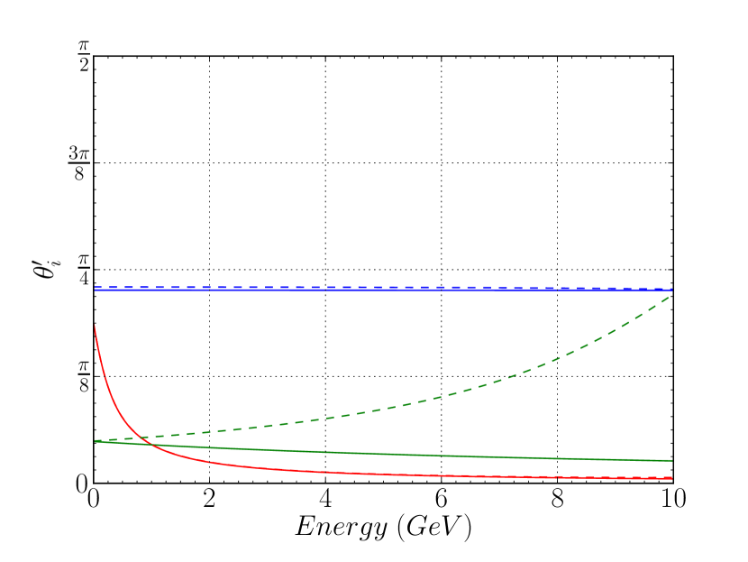
been plotted by numerically diagonalizing the Hamiltonian. It’s assumed the diagonalization matrix will have the same form as the standard parameterization of the PMNS mixing matrix.

The approximation introduced in Sec. III.1 implies that the $CP$ phase and $\theta^{\prime}_{a}$ do not vary much, if at all, due to interactions with matter (which can be observed in Fig. 9). It also implies certain characteristics of the variations of the other two mixing angles. From (18a), $\theta^{\prime}_{s}$ should be independent of the mass hierarchy, and taking the limit $a\to\infty$, then $\theta^{\prime}_{s}\to\frac{\pi}{2}$ ($0$) for $\nu$ ($\overline{\nu}$). This behavior is easily observed in Fig. 9. From (18b), $\theta^{\prime}_{r}$ should have similar asymptotic behavior as $\theta^{\prime}_{s}$ for normal

(a)

hierarchy, while it should reverse its behavior for inverted hierarchy. These features are approximately shown in Fig. 9, but at the energies shown, $\theta^{\prime}_{r}$ is not able to approach its asymptotic limit. Therefore, these results appear to agree with the approximation in Agarwalla et al. (2013a).

The effective neutrino masses are found from multiplying the eigenvalues of the Hamiltonian by $2E$. These plots are shown in Fig. 13 for NO$\nu$A. There are some interesting characteristics of these plots. The first and most obvious are two resonances referred to as the solar resonance and the atmospheric resonance which represent the condition for maximal oscillation probability. This phenomenon was first understood with the introduction of the MSW effect Wolfenstein (1978); Mikheev and Smirnov (1986). The first peak of $\sin^{2}(2\theta^{\prime}_{s})$ is the solar resonance and corresponds to an approach of $|\lambda_{1}|$ and $|\lambda_{2}|$ followed by a repulsion. The first peak of $\sin^{2}(2\theta^{\prime}_{r})$ is the atmospheric resonance and corresponds to an approach of $|\lambda_{2}|$ and $|\lambda_{3}|$ followed by a repulsion. If the absolute value of the mass eigenvalues cross, then no resonance can be seen there. If we don’t take the absolute value of the mass eigenvalues, then they will never cross each other. This is a wonderful example of level repulsion in quantum mechanics. For more details on these resonances, including a derivation of the resonance condition, see Wolfenstein (1978); Mikheev and Smirnov (1986); Smirnov (2005); Friedland (2001); Beringer (2012).

VI Conclusions

Predicted distributions for $\delta_{D}$, $J_{\nu}$, and $\theta_{a}$ were updated using the residual symmetries $\mathbb{Z}^{s}_{2}$ and $\overline{\mathbb{Z}}^{s}_{2}$. It was found that the greater uncertainty in the octant of $\theta_{a}$ for IH shown in Capozzi et al. (2013) forced the distributions of $\delta_{D}$ for IH to have nearly equal contributions on either side of $\delta_{D}=-90^{\circ}$. This had no significant effect on the distribution for $J_{\nu}$ and the prediction for $J_{\nu}$ has improved.

By including the effects of matter into the oscillation probabilities, it was shown in Sec. IV how NO$\nu$A stands

(a)

(a)

(a)

Figure 13: Effective masses for NO$\nu$A. The major focus of these plots should be on the solar and atmospheric resonances corresponding to a level repulsion. (a) $\nu$ and NH, (b) $\nu$ and IH, (c) $\overline{\nu}$ and NH, and (d) $\overline{\nu}$ and IH. Key: red $=\lambda_{1}$, blue $=\lambda_{2}$, green $=\lambda_{3}$, cyan-dashed $=\sin^{2}(2\theta_{s})$, and magenta-dashed $=\sin^{2}(2\theta_{r})$.

a good chance to determine the mass hierarchy if $\delta_{D}\in[\pi,2\pi]$ and the true hierarchy is normal, or if $\delta_{D}\in[0,\pi]$ and the true hierarchy is inverted. It was also shown that both NO$\nu$A and T2K may be capable of nailing down the octant of $\theta_{a}$.

The effects of matter were also shown to give rise to two resonances: the solar resonance and the atmospheric resonance. This behavior can be seen to agree with the approximation used throughout this work Agarwalla et al. (2013a).

VII Acknowledgments

The authors would like to thank Shao-Feng Ge for the contributions in the early stages of this work. W.W.R. would also like to thank Kendall Mahn for some helpful conversations. All plots in this paper were produced using matplotlib Hunter (2007). W.W.R. was supported in part by the National Science Foundation under Grant No. PHY-1068020. D.A.D. was supported in part by the U.S. Department of Energy under Award No. DE-FG02-12ER41830.

(a)

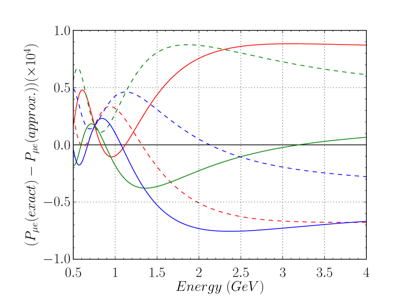
Appendix A Comparison with Solving for Matter Effects Exactly

Here a comparison is made between the approximation used Agarwalla et al. (2013a) and exact results found from numerically diagonalizing the Hamiltonian. Each plot for $P(\nu_{\mu}\to\nu_{e})$ and $P(\overline{\nu}_{\mu}\to\overline{\nu}_{e})$ above has been redone without any approximation. The plots below show the difference between these two methods. It’s clear that the approximation is indeed very good, with a maximum difference around $0.0001$.

(a)

Figure 15: Comparison between the exact results and the approximation used throughout the paper. For (a) NO$\nu$A and neutrinos, (b) NO$\nu$A and anti-neutrinos. Key: red $=(\delta_{D}=0)$, red-dash $=(\delta_{D}=\pi)$, green $=\mathbb{Z}^{s}_{2},\delta_{D}\in[0,\pi]$, green-dash: $=\mathbb{Z}^{s}_{2},\delta_{D}\in[\pi,2\pi]$, blue: $=\overline{\mathbb{Z}}^{s}_{2},\delta_{D}\in[0,\pi]$, blue-dash: $=\overline{\mathbb{Z}}^{s}_{2},\delta_{D}\in[\pi,2\pi]$.

References

- Abe et al. (2014) K. Abe et al. (T2K Collaboration), Phys.Rev.Lett. 112, 061802 (2014), arXiv:1311.4750 [hep-ex] .
- Capozzi et al. (2013) F. Capozzi, G. Fogli, E. Lisi, A. Marrone, D. Montanino, et al., (2013), arXiv:1312.2878 [hep-ph] .
- Forero et al. (2012) D. Forero, M. Tortola, and J. Valle, Phys.Rev. D86, 073012 (2012), arXiv:1205.4018v4 [hep-ph] .
- Gonzalez-Garcia et al. (2012) M. Gonzalez-Garcia, M. Maltoni, J. Salvado, and T. Schwetz, JHEP 1212, 123 (2012), arXiv:1209.3023v3 [hep-ph] .
- Ge et al. (2012) S.-F. Ge, D. A. Dicus, and W. W. Repko, Phys. Rev. Lett. 108, 041801 (2012), arXiv:1108.0964v3 [hep-ph] .
- Hanlon et al. (2014) A. D. Hanlon, S.-F. Ge, and W. W. Repko, Phys.Lett. B729, 185 (2014), arXiv:1308.6522 [hep-ph] .
- Jarlskog (1985) C. Jarlskog, Phys. Rev. Lett. 55, 1039 (1985).
- Kayser (2004) B. Kayser, eConf C040802, L004 (2004), arXiv:hep-ph/0506165v1 [hep-ph] .
- Kayser (2008a) B. Kayser, , 51 (2008a), arXiv:0804.1121 [hep-ph] .
- Kayser (2008b) B. Kayser, (2008b), arXiv:0804.1497 [hep-ph] .
- Agarwalla et al. (2013a) S. K. Agarwalla, Y. Kao, and T. Takeuchi, (2013a), arXiv:1302.6773v1 [hep-ph] .
- Patterson (2013) R. Patterson (NOvA Collaboration), Nucl.Phys.Proc. Suppl. 235-236, 151 (2013), arXiv:1209.0716 [hep-ex] .
- Agarwalla et al. (2013b) S. K. Agarwalla, S. Prakash, and S. U. Sankar, JHEP 1307, 131 (2013b), arXiv:1301.2574 [hep-ph] .
- Fogli et al. (2012) G. L. Fogli, E. Lisi, A. Marrone, D. Montanino, A. Palazzo, and A. M. Rotunno, Phys. Rev. D 86, 013012 (2012), arXiv:1205.5254v3 [hep-ph] .
- Wolfenstein (1978) L. Wolfenstein, Phys.Rev. D17, 2369 (1978).
- Mikheev and Smirnov (1986) S. Mikheev and A. Y. Smirnov, Nuovo Cim. C9, 17 (1986).
- Smirnov (2005) A. Y. Smirnov, Phys.Scripta T121, 57 (2005), arXiv:hep-ph/0412391 [hep-ph] .
- Kimura et al. (2002a) K. Kimura, A. Takamura, and H. Yokomakura, Phys.Rev. D66, 073005 (2002a), arXiv:hep-ph/0205295 [hep-ph] .
- Zaglauer and Schwarzer (1988) H. Zaglauer and K. Schwarzer, Z. Phys. C40, 273 (1988).
- Kimura et al. (2002b) K. Kimura, A. Takamura, and H. Yokomakura, Phys.Lett. B537, 86 (2002b), arXiv:hep-ph/0203099 [hep-ph] .
- Arafune et al. (1997) J. Arafune, M. Koike, and J. Sato, Phys.Rev. D56, 3093 (1997), arXiv:hep-ph/9703351 [hep-ph] .
- Freund (2001) M. Freund, Phys.Rev. D64, 053003 (2001), arXiv:hep-ph/0103300 [hep-ph] .
- Peres and Smirnov (2004) O. Peres and A. Y. Smirnov, Nucl.Phys. B680, 479 (2004), arXiv:hep-ph/0309312 [hep-ph] .
- Akhmedov et al. (2004a) E. K. Akhmedov, R. Johansson, M. Lindner, T. Ohlsson, and T. Schwetz, JHEP 0404, 078 (2004a), arXiv:hep-ph/0402175 [hep-ph] .
- Akhmedov et al. (2004b) E. K. Akhmedov, M. Tortola, and J. Valle, JHEP 0405, 057 (2004b), arXiv:hep-ph/0404083 [hep-ph] .
- Akhmedov and Niro (2008) E. K. Akhmedov and V. Niro, JHEP 0812, 106 (2008), arXiv:0810.2679 [hep-ph] .
- Cervera et al. (2000) A. Cervera, A. Donini, M. Gavela, J. Gomez Cadenas, P. Hernandez, et al., Nucl.Phys. B579, 17 (2000), arXiv:hep-ph/0002108 [hep-ph] .
- Dwyer (2013) D. A. Dwyer (Collaboration for the Daya Bay), (2013), arXiv:1303.3863 [hep-ex] .
- Hagiwara et al. (2011) K. Hagiwara, N. Okamura, and K.-i. Senda, JHEP 1109, 082 (2011), arXiv:1107.5857 [hep-ph] .
- Friedland (2001) A. Friedland, (2001), arXiv:hep-ph/0106042 [hep-ph] .
- Beringer (2012) J. Beringer (Particle Data Group), Phys. Rev. D 86, 177 (2012).
- Hunter (2007) J. D. Hunter, Computing In Science & Engineering 9, 90 (2007).