Near-Stability of a Quasi-Minimal Surface Indicated Through a
Tested Curvature Algorithm
Abstract
We decrease the mean curvature and area of a variable surface with a fixed boundary by iterating a few times through a curvature-based variational algorithm. For a boundary with a known minimal surface, starting with a deliberately chosen non-minimal surface, we achieve up to 65 percent of the total possible decrease in area. When we apply our algorithm to a bilinear interpolant bounded by four non-coplanar straight lines, the area decrease by the same algorithm is only percent of the original value. This relative stability suggests that the bilinear interpolant is already a quasi-minimal surface.
I Introduction
In a variational problem, we write the form (termed ansatz) of a quantity to be minimized in such a way that what remains to be found is the value(s) of the variational parameter(s) introduced in the ansatz. An important application of the variational approach is to find characteristics of a surface (called a minimal surface) locally minimizing its area for a known boundary.
Minimal surfaces initially arose as surfaces of minimal surface area subject to some boundary conditions, a problem termed Plateau’s problemOsserman1986 ; Nitsche1989 in variational calculus. Initial non-trivial examples of minimal surfaces, namely the catenoid and helicoid, were found by Meusnier in 1776. Later in 1849, Joseph Plateau showed that minimal surfaces can be produced by dipping a wire frame with certain closed boundaries into a liquid detergent. The problem of finding minimal surfaces attracted mathematicians like Schwarz Schwarz (who investigated triply periodic surfaces with emphasis on the surfaces called D (diamond), P (primitive), H (hexagonal), T (tetragonal) and CLP (crossed layers of parallels)), Riemann Osserman1986 , Weierstrass Osserman1986 and R. Garnier Garnier . Later, significant results were obtained by L. Tonelli Tonelli , R. Courant Courant1 Courant2 , C. B. Morrey Morrey1 Morrey2 , E. M. McShane Shane , M. Shiffman Shiffman , M. Morse MT , T. Tompkins MT , Osserman Osserman1970 , Gulliver Gulliver , Karcher Karcher and others.
The characteristic of a minimal surface resulting from a vanishing variation in its area is that its mean curvature should be zero throughout; see, for example, section 3.5 of ref. docarmo for the partial differential equation (PDE) this demand implies. This results in a prescription that to find a minimal surface we should find a surface for which the mean curvature function is zero at each point of the surface. Numerically, we have to find a zero for each set of values, which means we have to solve a large number of problems on a large grid. In converting this problem into a variational form we minimize the mean square functional of the mean curvature numerator i.e. (given below by eq. (10)) with respect to our variational parameter. This functional is more convenient than minimizing directly the area functional which has a square root in the integrand, but has the same extremal (i.e. a surface where this alternative functional is zero) as that of the area. This alternative can be compared with Douglas’ suggestion of minimizing the Dirichlet integral that has the same extremal as the area functional. (A list of other possibilities of such functionals can be found in refs.MUComparative ; Chen2009 .) An additional advantage is that for we know the value (that is, zero) to be achieved; for the area integral we do not know before calculations the target minimum value.
In an earlier work vms , for a boundary composed of four straight lines, we reduced the curvature and area of an initial surface chosen to be a bilinear interpolant. In this paper we took the ansatz for change in the surface to be proportional to the numerator of the mean curvature function for the surface; other factors in the change were the variational parameter, a function of the surface parameters (not to be confused with the variational parameters) whose form vanishes at the boundary and a vector assuring that we add a 3-vector to the original surface in 3-dimensions. In this paper we make an iterative use of the same ansatz, written in eq. (6) below, to improve on this initial surface along with two other surfaces. Now we calculate afresh our variational parameter for each iteration . An important feature of our work is that at each iteration, the function we minimize (that is of eq. (10)), remains a polynomial in our variational parameter . We used a computer algebra system to carry out our calculations and thus computational problems stopped us from actually implementing all the iterations. We somewhat avoided this impasse for a simpler case using a curve rather than a surface. This replaced the target flat surface by a straight line and the mean curvature by a second derivative. In this case too we had to eventually minimize a polynomial. In each case, the resulting value of the variational parameter specifies the curve or surface at each iteration.
In this paper, before reducing the area of the bilinear interpolant for which no minimal surface is completely known, we first considered two cases (a hemiellipsoid bounded by an elliptic curve and a hump-like surface spanned by four straight lines) where we already know a minimal surface for the boundary but we deliberately start with a non-minimal surface for the same boundary. We did this to find what fraction of the total possible area decrease (area of the starting non-minimal surface minus that of the known minimal surface) we achieve in the computationally manageable few iterations. If the target surface is flat, achieving it is sufficient but not necessary. This is because, at least according to the traditional definition of a minimal surface as a surface with zero mean curvature, for a fixed boundary we may have more than one minimal surface; vanishing mean curvature is a solution of an equation obtained by setting to zero the derivative of the surface with respect to the variational parameter in its modified expression and thus a solution surface can be guaranteed to be only a locally minimal surface in the set of all the surfaces generated by this modification and hence is not unique. Thus another question about our algorithm is whether or not it gets stuck in some other (locally) ”minimal” curve or surface before it reaches the straight line or a flat surface. We tested our ansatz for two cases with known minimal surfaces; of course for neither case the initial surface we chose was a minimal one.
After testing in this way our algorithm, we used it to find a surface of smaller mean curvature and area for a boundary for which no minimal surface is known. For such a case we have tried to judge if an initial surface chosen with a fixed boundary is stable or quasi-stable against the otherwise decreasing areas that our algorithm can generate and took the resulting near stability as an indication that our initial surface is a quasi-minimal surface for our boundary. In this paper, we report area reductions in a number of iterations to strengthen our premise. We have compared our previous ansatz with a simpler alternative (see eq. (25) below) to point out that the ansatz we used can be repeatedly used, which is not the case with each possible ansatz, and thus is a non-trivial feature of the ansatz we used and are further using in this paper. The ansatz gives a significant reduction in areas in case of hemiellipsoid and hump-like surfaces (with already known minimal area) in computationally manageable few iterations whereas for the bilinear interpolant (a quasi-minimal surface of unknown minimal area) the decrease remains less than 0.1 percent of the original area. This also enabled us to numerically work out differential geometry related quantities for these surfaces. We have not been able to achieve a minimal surface within our computationally manageable resources. But, considering the possibility of implementing the same broad algorithm differently (maybe with a better computer program or with less reliance on the computationally demanding algebra system), our present work may be a test-bed for improved detailed algorithms aimed at computing minimal surfaces.
Our work can be compared to others Monterde2004 ; MonterdeUgail2004 who have converted Dirichlet integrals into a system of linear equations which can be solved Monterde2004 ; Chen2009 to obtain extremals of a Dirichlet integral and thus surfaces of reduced area of a class of Bézier surfaces FD . Chen2009 employs the Dirichlet method and the extended blending energy method to obtain an approximate solution of the Plateau- Bézier problem by introducing a parameter in the Extended Dirichlet Functional (compare eq. (4) of the ref. Chen2009 with our eq. (10)). Determining this parameter gives all the inner control points obtained directly as the solution of a system of linear equation. In our case, determining the variational parameter gives us variationally improved surfaces. The constraint that the mean curvature is zero is too strong and in most of the cases there is no known Bézier surface Chen2009 with zero mean curvature.
Xu et al. Xu2009 study approximate developable surfaces and approximate minimal surfaces (defined as the minimum of the norm of mean curvature) and obtain tensor product Bézier surfaces using a nonlinear optimization algorithm. Hao et al. HaoYong2013 find the parametric surface of minimal area defined on a rectangular parameter domain among all the surfaces with prescribed borders using an approximation based on Multi Resolution Method using B-splines. Xu and Wang Xu2010 study quintic parametric polynomial minimal surfaces and their properties. Pan and Xu QuingPan2011 construct minimal subdivision surfaces with given boundaries using the mean curvature flow, a second order geometric PDE, which is solved by a finite element method. For some possible applications of minimal or quasi-minimal surfaces spanning bilinear interpolants and for a literature survey, one can read the introductory section of our work vms on Variational Minimization of String Rearrangement Surfaces and dabm2013 on Coons Patch Spanning a Finite Number of Curves.
This paper is organized as follows: In section II we first point out the variational aspect of the proof of the connection between area reduction and vanishing mean curvature to provide motivation for our ansatz. We give related definitions and the variational algorithm based on our ansatz containing the numerator of the mean curvature function to reduce the area of a surface spanned by a fixed boundary (including the boundary composed of a finite number of given curves). In section III, we first present a one-dimensional analogue of our ansatz of eq. (6) which is applied to a curve of given length. For this simplest case, we report implementing eight iterations to get curves of reduced lengths. This is followed by applying our technique to a hemiellipsoid surface (with an ellipse for a boundary) and a hump-like surface (spanned by four coplanar straight lines) to test the algorithm for the number of iterations it takes to return a surface of significantly reduced area for a boundary for which a minimal surface is known; in these complicated cases we could implement fewer iterations. The technique is then applied to the bilinear interpolant bounded by four non-coplanar straight lines, for which a minimal surface is not known. A comparison of root mean square of mean curvature and Gaussian curvature in the three cases is also provided for further analysis of certain properties of these surfaces. Based on this comparison, results and remarks are presented in the final section IV.
II Motivation for the Ansatz
Our goal is to decrease the area functional docarmo ; Goetz
| (1) |
of a locally parameterized surface . Here is a domain over which the surface is defined as a map, with the boundary curve given by for . and are the partial derivatives of with respect to and . The normal variation of ( is the union of the domain with its boundary ), determined by a differentiable function , is the map defined by
| (2) |
For each fixed , the map given by is a parameterized surface. Let and denote the first fundamental magnitudes docarmo of and , the second fundamental magnitudes of , the unit normal to and , the mean curvature function of the surface . Ref. docarmo shows that the derivative of the area integral
| (3) |
at is
| (4) |
with
| (5) |
For our chosen initial non-minimal surfaces, is non-zero. The basic idea of our algorithm is that it is always possible to decrease the area and thus to get a negative value of by choosing the differential function to be proportional to the mean curvature function . Because our target is only a sign of the product , we simplify our work by using only the numerator of the mean curvature given by (5). (This is also done in ref. BCDH following ref. Osserman1986 that “for a locally parameterized surface, the mean curvature vanishes when the numerator of the mean curvature is equal to zero”.) Thus our iterative scheme for the successive surfaces is
| (6) |
where is our variational parameter and
| (7) |
with chosen so that the variation at the boundary curves is zero. denotes the numerator of the mean curvature function eq. (5) of the non-minimal surface and is given by
| (8) |
Our ansatz in eq. (6) can be compared with the arbitrary variation of eq. (2) to see the choices made in our ansatz. For , we denote by and the fundamental magnitudes and by the numerator of the unit normal to the surface . The subscript is used not only to denote the numerator of the quantities but also to denote the iteration. For non-zero each of the above functions of an iterative surface is also a function of the corresponding in addition to usual dependence on the parameters and of the surface. The functional dependence on is always a polynomial one. That is,
| (9) |
We have written in the introduction that in place of the problematic area functional, what we minimize to find is
| (10) |
Because of eq. (9), in our expression for is also a polynomial in with real coefficients of for that we call ; there are no powers of higher than 10 in the polynomials as can be seen from the expressions for , and which are quadratic in and , and which are cubic in . Integrating (numerically if necessary) these coefficients with respect to and in the range we get that we minimize with respect to . The resulting value of completely specifies a surface . For this value of , the new surface has less mean curvature than the mean curvature
| (11) |
of the surface . This surface is also expected to have less area and in our actual calculations we found that as we decrease our alternative functional , the area functional of the surface spanning our fixed boundary also decreases. The mean curvature of both our starting surface and the one achieved after one variational area reduction remains non-zero and we re-use our variational algorithm for the resulting surface a number of times. Mean curvature tells how much the two principal curvatures docarmo of the surface cancel. To get an estimate of the absolute sizes of the principal curvatures we also calculated for each iteration the mean square () of Gaussian curvature docarmo for and . This we call , given by the following expression:
| (12) |
where is the numerator of the Gaussian curvature . Gaussian curvature is the product of principal curvatures and mean curvature is average of the principal curvatures. Thus a ratio of Gaussian curvature and square of mean curvature is dimensionless. Using eqs. (10) and (12), this ratio is
| (13) |
Now for , we compute , and and denote the area integral eq. (1) as which is given by the following expression
| (14) |
The ansatz eq. (6), for the first order reduction in the area of a non-minimal surface is
| (15) |
where is our variational parameter. Here are given by eqs. (7), (9) and is the unit normal to the non-minimal surface for . For , the ratio (16) of the of Gaussian curvature to the of mean curvature is given by
| (16) |
where is the numerator of the Gaussian curvature . With the above notation, eq. (1) becomes, for ,
| (17) |
For in eq. (6) gives us the surfaces , of reduced area and related quantities may be computed from eqs. (7) to (14). In order to see a geometrically meaningful (relative) change in area we calculate the dimensionless area ratios. For the cases with known minimal surface, let be the initial area and the area of the known minimal surface (which we took, for these ratio calculations, as the corresponding flat surface; the subscript reminds us of this). We can define the maximum possible change to be achieved as . Let for be the area of the surface obtained through the iteration. Then the difference of the areas in the and iteration, with , is denoted by . When we know the minimal surface, the percentage decrease in area can be computed by multiplying the quotient of and by . Thus we have
| (18) |
When we do not know the minimal surface, the percentage decrease in area can be computed by using
| (19) |
III The Efficiency Analysis of the Ansatz eq. (6)
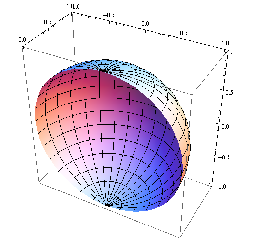
In this section we apply the technique introduced in section II to reduce the area of a variety of non-minimal surfaces. We start by reporting calculations for a hemiellipsoid bounded by an elliptic curve for which a minimal surface is the elliptic disc. This starting non-minimal surface is given by the parametrization
| (20) |
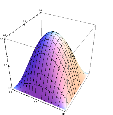
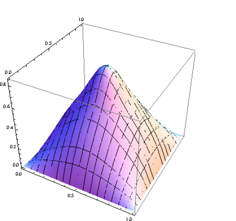
where , are constants and and as shown in Fig. 1. For a second case, we took the starting surface as a hump-like surface spanned by four arbitrary straight lines with parametrization
| (21) |
where as shown in Fig. 2. The target minimal surface in this case is also a flat surface, but the boundary is instead a square. The minimum area in this second case is that of a square of unit length. Our success (reported below) in significantly reducing the area in these known cases suggests it is interesting to find and analyze area reductions in surfaces for which no minimal surface is known. Linear interpolant in the one-dimensional case (a straight line) is already minimal. But the mean curvature function for the bilinear interpolant spanning a non-planar boundary is not zero, meaning the derivative of the area function with respect to a variational parameter is non-zero. The curvature-based algorithm we suggest manages to utilize this non-zero mean curvature and area derivative to decrease both of these quantities. For definiteness, we took the corners
| (22) |
of our bilinear interpolant as
| (23) |
for a real scalar . For this case, the bilinear interpolant is the following bilinear mapping from to :
| (24) |
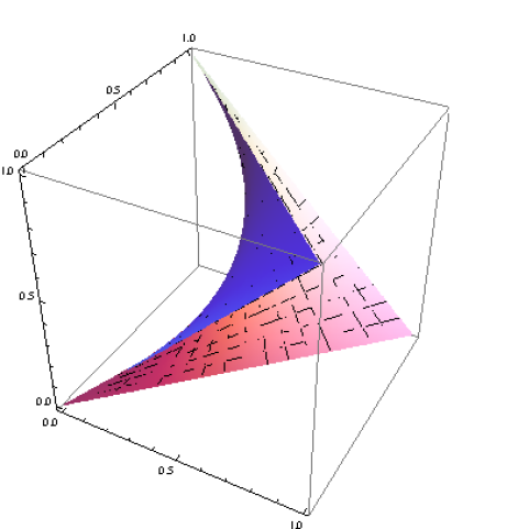
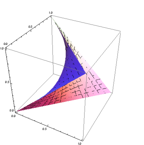
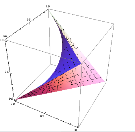
Since is the only scale in our problem, geometrical properties do not depend on the actual value of we choose; the argument is straightforward for the dimensionless ratios we report. Thus we take the simplest choice of taking ; for this choice the bilinear interpolant is shown in Fig. 3.
In case of a hemiellipsoid, to check if some alterations in our algorithm can be introduced, we replaced, in our ansatz for a change in surface, the mean curvature function by a constant chosen as one. An argument shows that this simple algorithm can not be iterated: with starting value of and a convenient choice of and , , the ansatz eq. (6) reduces to the following expression
| (25) |
where is now the variational parameter. Any further iteration of this algorithm would only change the value of but not the form of the resulting surface. But the value is uniquely given by our minimization. Thus for iterating our algorithm we restored the non-trivial original mean curvature numerator defined as above by eq. (8). The resulting decreases in mean curvature and areas from the above mentioned starting surfaces are reported in the four subsections below. A comparison can be seen in table 2.
III.1 The 1-Dimensional Analogue of the Curvature Algorithm Applied to a Curve of a Given Length
Before finding what our algorithm(s) yield for surfaces, we wrote a program for the variational problem of reducing arc length, targeting this time the straight line joining the end points of the curve. For this one dimensional variational problem our ansatz for successive curves joining the same two ends may be written in the form:
| (26) |
where
| (27) |
is chosen so that it is zero at and . Here, is the iteration number. is a unit vector in the direction normal to the curve, which practically means we take the transverse displacement from the straight line joining the two ends. In place of the numerator of the mean curvature for the surface case, we take here to be ordinary curvature which is the second derivative with respect to the curve parameter . When the technique was applied to a starting curve
| (28) |
it gave the following expressions for variationally improved curves
| (29) | |||
| (30) | |||
| (31) | |||
| (32) | |||
| (33) | |||
| (34) | |||
| (35) | |||
| (36) |
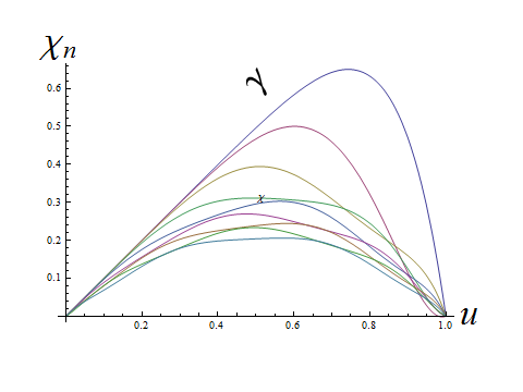
Corresponding lengths of these curves are , , , , , , , and . Percentage decreases in the lengths are denoted by
| (37) |
and are reported in table 1. Fig. 4 shows the graphs of all the curves which we could achieve before exhausting the limit of available computer resources. It can be seen from the second column of table 1 that the length of the sequence of curves is getting closer and closer to the shortest (unit) length joining the two ends. We also report in the next column the corresponding values of the variational parameter that gives these lengths.
The decreasing lengths of the variationally improved curves along with percentage decreases in length given by () for the corresponding optimal value of our variational parameter .
| 1.7329 | |||
| 1.46525 | 36.5206 | 0.132653 | |
| 1.30988 | 21.1996 | 0.070933 | |
| 1.24103 | 9.3933 | 0.061298 | |
| 1.20133 | 5.41714 | 0.048743 | |
| 1.16958 | 4.33218 | 0.044937 | |
| 1.1459 | 3.2307 | 0.039161 | |
| 1.12682 | 2.60332 | 0.037408 | |
| 1.11081 | 2.18471 | 0.034467 |
III.2 The Hemiellipsoid Results
For constants and and , fundamental magnitudes, mean curvature and the area of the initial surface hemiellipsoid of eq. (20) are
| (38) | ||||
| (39) | ||||
| (40) | ||||
| (41) | ||||
| (42) | ||||
| (43) | ||||
| (44) | ||||
| (45) |
In particular for , these quantities reduce to , . The corresponding function is defined as
| (46) |
Since the success of our algorithm depends only on the sign of the derivative of area in eq. (4), we can modify the previously used changes in our surface that do not alter the signs of the area derivative. Utilizing this freedom, we replaced the variable normal to the surface by a fixed unit vector that gives the same sign of the area derivative. For our hemiellipsoid case, has this property and we replaced the normal to the surface by this simpler 3-vector. Below we give the reduction in area of the hemiellipsoid eq. (20) for the two cases, one for which is replaced by and one for which is numerator of the mean curvature. Replacing by in eq. (7) along with (46) gives the first variational surface as
| (47) |
Thus the coefficients of in the expansion of the usual numerator of the mean curvature and the mean square of the mean curvature (eq. (10) for ) are given by
| (48) | ||||
| (49) | ||||
| (50) | ||||
| (51) | ||||
| (52) |
Minimizing with respect to gives us , so that
| (53) |
We found and thus the percentage decrease in area is given by . Similarly we calculated
| (54) |
In this case and hence
| (55) |
Here, and . The percentage decrease for the full area reduction at this stage is . Continuing the process, we find the mean square mean curvature for . Here
| (56) |
In this case and this gave us (a lengthy expression not reproduced here) for which the area comes out to be , . We found . These results are presented in the table 2. Below we give results for the reduction in area of the hemiellipsoid eq. (20) for which we restored the non-trivial actual mean curvature numerator . In this case we have been able to produce only two iterations. For , and the expressions for , the first variational surface and , mean square of the mean curvature, are
| (57) | ||||
| (58) | ||||
| (59) |
In this case . Accordingly, the first variational surface is given by
| (60) |
The percentage decrease in the mean curvature of the numerator of the mean curvature is 74.1475. Area and the percentage decrease in area , as summarised below in table 2. Continuing the process as above we find the dependence on our variational parameter of the mean square of the mean curvature is
| (61) |
Here and related results are summarized in table 2. It can be seen from table 2 that this choice of gives a better reduction in the area even for the first iteration.
III.3 A Hump-Like Surface (21) Spanned by Four Boundary Coplanar Straight Lines
We apply the ansatz eq. (6) along with eq. (7) mentioned in section II to the surface given by eq. (21) bounded by four coplanar straight lines . A function whose variation at the boundary curves is zero is given by
| (62) |
A convenient possible choice for the alternative to the unit normal to this surface is which makes a small angle with this unit normal and thus does not change the sign of the area derivative. The surface given by eq. (21) is a non-minimal surface and the -plane bounded by is a minimal surface spanning its boundary. The fundamental magnitudes of the initial surface eq. (21) are
| (63) | ||||
| (64) | ||||
| (65) | ||||
| (66) | ||||
| (67) | ||||
| (68) |
Thus, eq. (8) for , along with eqs. (63) to (68) gives
| (69) |
as shown in Fig. 5.
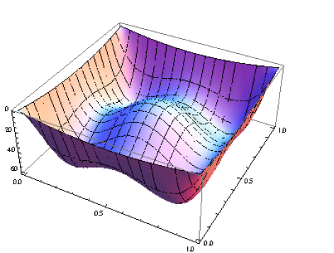
Substituting the value of from eq. (69) along with eq. (62) in eqs. (6) (7) for gives us the following expression
| (70) |
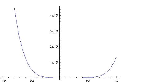
Denoting the fundamental magnitudes for this variational surface by , , , , , and plugging in these values in eq. (9) for , we find the expression for , mean curvature of . These fundamental magnitudes, the mean curvature and the coefficients of in the expansion of are given in Appendix A. is a polynomial in and thus is polynomial in as well. We find the non-zero coefficients of and integrate these coefficients for as mentioned in eq. (10) to get an expression for the mean square of the mean curvature (10) for , as a polynomial in . This is
| (71) |
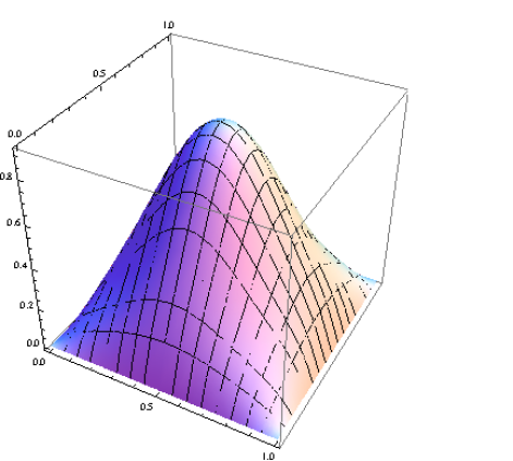
shown in Fig. 6. Minimizing this polynomial for gives us . We find the variationally improved surface eq. (15) for this minimum value of , that is,
| (72) |
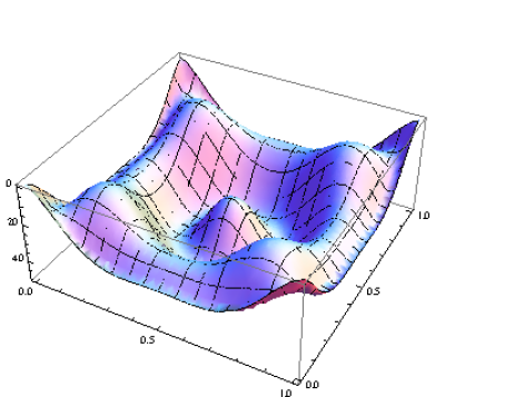
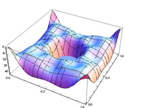
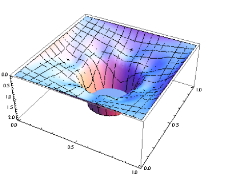
shown in Fig. 7. For this the mean curvature of is shown in Fig. 8. The initial area of the surface (using eq. (17)) is and that of the surface (72) (using eq. (14)) is for . The percentage decrease in the original area in this case is . Substituting (shown in Figure 8) in eq. (7) along with eq. (62) for in eq. (6) results in an expression for the variational surface . We find the fundamental magnitudes , , , , , for this variational surface and insert these fundamental magnitudes in eq. (9) to get the expression for , mean curvature of , and thus mean square of mean curvature (eq. (10) for ) gives the following expression,
| (73) |
Minimizing this expression results in . For this we find the variationally improved surface shown in Fig. (9). The numerator of the mean curvature of is shown in Fig. 10 and the quantity is shown in Fig. 11. A summary of related results is provided in table 2.
III.4 The Bilinear Interpolant (24) Spanned by Four Boundary Non-Coplanar Straight Lines
In the previous subsection we have applied the algorithm eq. (6) along with eq. (7) (section II) to a surface for which the corresponding minimal surface is known. We have judged that our algorithm can significantly decrease area where the area can be decreased. Below, we apply this algorithm to an important class of surfaces, namely the bilinear interpolant where the corresponding minimal area is not explicitly known. Specifically, we have taken the initial surface given by eq. (24) for . It is bounded by four non-coplanar straight lines. A convenient alternative for the unit normal in eq. (6) is , making a small angle with the unit normal to the surface given by eq. (24). The corresponding function assuring that the variation of the surface at the boundary curves at vanishes is given by
| (74) |
The surface given by (24) for is a non-minimal surface spanned by a boundary composed of non-coplanar straight lines. The fundamental magnitudes of this initial surface are
| (75) |
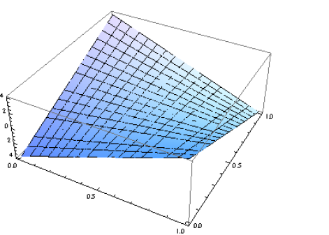
For , eq. (8) along with eq. (75) gives
| (76) |
as shown in the Fig. 12.
The variationally improved surface eq. (6) along with its fundamental magnitudes as functions of and are
| (77) | ||||
| (78) | ||||
| (79) | ||||
| (80) | ||||
| (81) | ||||
| (82) | ||||
| (83) |
Thus, eq. (9) along with eqs. (78) to (83) gives an expression for and hence the coefficients of for in the expansion of as mentioned in the eq. (9), which are given in Appendix B. is a polynomial in and thus is polynomial in as well. We find the non-zero coefficients of and integrate these coefficients for , as mentioned in eq. (10), to get an expression for the mean square of mean curvature as a polynomial in , given by
| (84) |
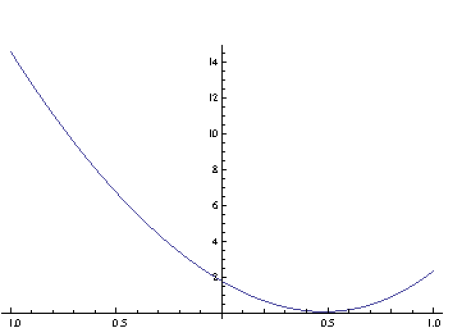
Minimizing this polynomial for gives us . The mean square of mean curvature of the surface as a function of is shown in Fig. 13.
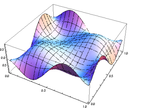
The mean curvature of is shown in Fig. 15.
The initial area of the surface (eq. (24)) (using eq. (17)) is and that of surface (85) is . In a similar way, we find the second order variation of the bilinear interpolant whose mean square of mean curvature, according to eq. (10), is
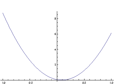
| (86) |
as shown in Fig. 16 as a function of . (Details are given in Appendix B). Here for which the variational surface is shown in Fig. 17 and given in Appendix B. The curvature of this surface is shown in Fig. 18.
The initial area (calculated using eq. (14)) of surface of eq. (24) is and that (eq. (14) for ) of surface of eq. (85) is for . The area (eq. (14) for ) of surface of eq. (103) is . The percentage decrease in area with respect to that of eq. (85) is 0.004382. We have not been able to find higher order variational surfaces for as in this case our computer program becomes unresponsive for higher iterations. However to foresee that a further reduction is possible, the variational quantity for is shown in Fig. 19. The algorithm reduces area less significantly for the bilinear interpolant. We suggest this relative stability indicates that the bilinear interpolant is a quasi-minimal surface. The ratio of of Gaussian curvature to the of the mean curvature obtained for successive surfaces decreases for the hemiellipsoid, whereas this ratio increases for the hump-like surface and the bilinear interpolant. Moreover, it can be seen from table 2 that by using the actual , the percentage decrease in area of the hemiellipsoid is slightly more than the decrease obtained by replacing by 1. A summary of these results is presented in table 2.
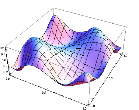
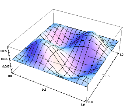
A summary of results for the surfaces , with starting surface written in the first column. are the decreasing areas, and () are the percentage decreases in areas. are the of Gaussian curvature and are the of the mean curvature. The last column reports the optimal value of our variational parameter for each of the cases.
| Hemiellipsoid, Hump-Like Surface and Bilinear Interpolant | |||||
| Hemiellipsoid () | 6.28319 | - | - | 0.38985 | |
| 4.70625 | 50.1954 | - | 0.01369 | -0.35157 | |
| 4.4403 | 8.46711 | - | 0.01308 | 0.07064 | |
| 4.4025 | 1.20025 | - | 0.01307 | 0.02264 | |
| Hemiellipsoid | 6.28319 | - | - | 0.38985 | - |
| 4.32641 | 62.2861 | - | 0.19644 | 0.14825 | |
| 4.23731 | 2.83624 | - | 0.18095 | 0.02297 | |
| Hump-Like Surface | 2.49452 | - | - | 0.03456 | - |
| 2.11589 | 25.3341 | - | 0.05207 | 0.08893 | |
| 1.92788 | 12.58 | - | 0.09449 | 0.04409 | |
| Bilinear Interpolant | 1.280789 | - | - | 2.25 | - |
| 1.27936 | - | 0.11157 | 58.9258 | 0.48364 | |
| 1.2793 | - | 0.00461 | 272.152 | 0.0881 | |
IV Conclusions
We have discussed how to reduce the surface area of the non-minimal surfaces given by eqs. (20), (21) and (24) by using a variational technique with an appropriate number of iterations to improve the surfaces . The first two cases are meant to test our curvature algorithm and the third one applies this algorithm to a surface for which there is no corresponding known minimal surface. The percentage decrease in area of the hemiellipsoid eq. (20) is given for two cases: one for which is replaced by 1 and one for which is the usual numerator of the mean curvature defined by eq. (8). In the notation of eq. (18), the area reductions in the former case are and , and in the latter case are and . For the hump-like surface eq. (21), the percentage decreases in area are and . This indicates that the algorithm attains at least a local minimum of the area in these two cases. The percentage decrease (resulting through the corresponding slightly different definition given by eq. (19)) in area of the surface eq. (24) is much less i.e. and . This means that in the case of bilinear interpolant with unknown minimal surface, the variational improvement does not result in a significant decrease in the area. This saturation indicates that the bilinear interpolant is at least a local minima. Thus the bilinear interpolant is indicated as (or may well be) a critical point of the area.
Appendix A Expressions Used in Section III.3
Here , , , , , denote the fundamental magnitudes of the first variational surface obtained by plugging eq. (21) in eq. (6) for where denotes the coefficient of () in the polynomial expansion of (eq. (9)) for . is the numerator of the mean curvature of the surface .
| (87) | ||||
| (88) | ||||
| (89) | ||||
| (90) | ||||
| (91) | ||||
| (92) |
| (93) |
| (94) |
| (95) |
| (96) |
| (97) |
Appendix B Expressions Used in Section III.4
Here is the numerator of the mean curvature of the surface obtained by plugging eq. (24) in eq. (6) for where denotes the coefficient of () in the polynomial expansion of (eq. (9)) for . The variational surface is obtained by plugging eq. (85) in eq. (6) for . Minimizing the polynomial in eq. (86) for gives us , which results in the surface of lesser area given by .
| (98) | ||||
| (99) | ||||
| (100) | ||||
| (101) | ||||
| (102) |
| (103) |
| (104) |
References
- [1] R. Osserman. A survey of Minimal Surfaces. Dover Publications Inc., 1986.
- [2] J. C. C. Nitsche. Lectures on Minimal Surfaces. Cambridge University Press, 1989.
- [3] H.A. Schwarz. Gesammelte Mathematische Abhandlungen. 2 Bände. Springer, 1890.
- [4] R. Garnier. Le problème de Plateau. Annales Scientifiques de l’E.N.S., 3(45):53–144, 1928.
- [5] L. Tonelli. Sul problema di Plateau, I & II. Rend. R. Accad. dei Lincei, 24:333–339, 393–398, 1936.
- [6] R. Courant. Plateau’s problem and Dirichlet’s principle. Ann. of Math., 38:679–725, 1937.
- [7] R. Courant. Dirichlet’s principle, conformal mapping and minimal surfaces. Springer, 1977.
- [8] C. B. Morrey. The problem of Plateau on a Riemannian manifold. Ann. of Math., (2)49:807–851, 1948.
- [9] C. B. Morrey. The higher-dimensional Plateau problem on a Riemannian manifold. Proc. Nat. Acad. Sci. U.S.A., 54:1029–1035, 1965.
- [10] E. J. Shane. Parameterization of saddle surfaces, with applications to the problem of Plateau. Trans. Amer. Math. Soc., 35:716–733, 1933.
- [11] M. Shiffman. The Plateau problem for non-relative minima. Annals of Math., 40:834–854, 1939.
- [12] Morse and Tompkins. Minimal surfaces of non-minimum type by a new mode of aproximation. Annals of Math., 42:443–472, 1941.
- [13] R. Osserman. A proof of the regularity everywhere of the classical solution to Plateau’s problem. Annals of Math., 91:550–569, 1970.
- [14] R. Gulliver. Regularity of minimizing surfaces of prescribed mean curvature. Annals of Math., 97:275–305, 1973.
- [15] H. Karcher. The triply periodic minimal surfaces of A. Schoen and their constant mean curvature companions. Man. Math., 64:291, 1989.
- [16] M. Do Carmo. Differential Geometry of Curves and Surfaces. Prentice Hall, 1976.
- [17] J. Monterde and H. Ugail. A comparative study between biharmonic Bézier surfaces and biharmonic extremal surfaces. International Journal of Computers and Applications, 31(2):90–96, 2009.
- [18] Xiao-Diao Chen, Gang Xu, and Yigang Wanga. Approximation methods for the Plateau-Bézier problem. In Computer-Aided Design and Computer Graphics, 2009. CAD/Graphics ’09. 11th IEEE International Conference on, pages 588–591, 2009.
- [19] D. Ahmad and B. Masud. Variational minimization on string-rearrangement surfaces, illustrated by an analysis of the bilinear interpolation. arXiv:1205.3216v1 [math.DG], 2012, accepted for a publication by Applied Mathematics and Computation, Elsevier.
- [20] J. Monterde. Bézier surfaces of minimal area: The Dirichlet approach. Computer Aided Geometric Design, 21:117–136, 2004.
- [21] J. Monterde and H. Ugail. On harmonic and biharmonic Bézier surfaces. Computer Aided Geometric Design, 21:697 – 715, 2004.
- [22] G. E. Farin and D. Hansford. Discrete Coons patches. Computer Aided Geometric Design, 16:691–700, 1999.
- [23] Gang Xu, Xiaodiao Chen, and Guozhao Wang. Weighted approximate developable minimal Bézier surfaces. Journal of Computational Information Systems, 5(4):1047–1052, 2010.
- [24] Yong-Xia Hao, Chong-Jun Li, and Ren-Hong Wang. An approximation method based on MRA for the quasi-plateau problem. BIT Numerical Mathematics, 53(2):411–442, 2013.
- [25] Gang Xu and Guozhao Wang. Quintic parametric polynomial minimal surfaces and their properties. Differential Geometry and its Applications, 28:697 – 704, 2010.
- [26] Qing Pan and Guoliang Xu. Construction of minimal subdivision surface with a given boundary. Computer-Aided Design, 43(4):374 – 380, 2011.
- [27] D. Ahmad and B. Masud. A Coons patch spanning a finite number of curves tested for variationally minimizing its area. Abstract and Applied Analysis, 2013, 2013.
- [28] A. Goetz. Introduction to Differential Geometry. Addison Wesley Publishing Company, 1970.
- [29] W. Businger, P. A. Chevalier, N. Droux, and W. Hett. Computing minimal surfaces on a transputer network. Mathematica Journal, 4:70–74, 1994.