Statistical mechanics of human resource allocation: A mathematical modeling of job-matching in labor markets

Abstract

We provide a mathematical model to investigate the human resource allocation problem for agents, say, university graduates who are looking for their positions in labor markets. The basic model is described by the so-called Potts spin glass which is well-known in the research field of statistical physics. In the model, each Potts spin (a tiny magnet in atomic scale length) represents the action of each student, and it takes a discrete variable corresponding to the company he/she applies for. We construct the energy to include three distinct effects on the students’ behavior, namely, collective effect, market history and international ranking of companies. In this model system, the correlations (the adjacent matrix) between students are taken into account through the pairwise spin-spin interactions. We carry out computer simulations to examine the efficiency of the model. We also show that some chiral representation of the Potts spin enables us to obtain some analytical insights into our labor markets.

1 Introduction

Apparently, humans (or labors) are the most important resources in our society. This is because they can produce not only various products and services in the society but also they contribute to the society by paying their taxes. For this reason, in each scale of society, say, from nation to companies or much smaller communities such as laboratory (or research group) of university, allocation of human resources is one of the essential problems. Needless to say, such appropriate allocation of human resource is regarded as a ‘matching problem’ between individuals and some ‘groups’ such as companies, and the difference among individuals in their abilities or preference makes the problem difficult.

A typical example of the human resource allocation is found in simultaneous recruiting of new graduates in Japan. Students who are looking for their jobs might research several candidates of companies to enter and send the application letter through the web site (what we call ‘entry sheet’). However, the students incline to apply to well-established companies, whereas they do not like to get a job in relatively small companies. This fact enhances the so-called ‘mismatch’ between labors (students) and companies. We can easily see the situation of job-searching process in Japan. At the job fair, we find that some booths could collect a lot of students (they are all wearing a dark suit even in midsummer!). On the other hand, some other booths could not attract the students’ attentions. Therefore, the job-matching itself is apparently governed by some ‘collective behavior’ of students. Namely, each student seems to behave by looking at their ‘neighbors’ and adapting to the ‘mood’ in their community, or they sometimes can share the useful information (of course, such information is sometimes extremely ‘biased’) about the market via Internet or social networking service.

In macroeconomics, there already exist a lot of effective attempts to discuss the macroscopic properties Aoki ; Boeri ; Roberto ; Fagiolo ; Neugart including so-called search theory Lippman ; Diamond ; Pissarides1985 ; Pissarides2000 . However, apparently, the macroscopic approaches lack of their microscopic view points, namely, in their arguments, the behavior of microscopic heterogeneous agents such as labors or companies are neglected.

To investigate the collective effects on the job-matching process from the microscopic view point, we have proposed several models and carried out computer simulations Chen ; Chen2 ; Chen3 by considering some ‘aggregate data set’ for the labor market.

In our previous successive studies Chen ; Chen2 ; Chen3 , we succeeded in evaluating the macroscopic quantities such as unemployment rate $U$ and labor shortage ratio $\Omega$ from the microscopic view point. However, these our studies depend on numerical (computer) simulations for relatively small system size to calculate these quantities, and we definitely need some mathematically rigorous approaches to find the universal fact underlying in the job-matching process of labor markets. It is also important issue to be considered that we should take into account correlation between agents (students) when we consider the job-matching process in realistic labor markets. However, in our previous studies Chen ; Chen2 ; Chen3 , we have neglected the correlation in our modeling.

Motivated by the above background and requirement, here we propose a mathematical toy model to investigate the job-matching process in Japanese labor markets for university graduates and investigate the behavior analytically. Here we show our preliminary limited results for the typical behavior of the market.

This paper is organized as follows. In section 2, we briefly review our previous study on the urn model with disorder Inoue2008 and several remarkable properties of the model such as Bose-Einstein condensation. We also mention that the urn model cannot take into account the interactions between agents. In section 3, we introduce our toy model, the so-called Potts model, and explain several macroscopic quantities. Our preliminary results for several job-searching and selection scenarios by students and companies are shown in section 4. The last section 5 is summary and discussion.

2 Urn models and Bose condensation: A short review

As a candidate of describing the resource allocation problem, we might use the urn models. In this model, one can show that a sort of Bose condensation takes place. Hence, here we introduce the urn model with a disorder and explain several macroscopic properties according to the reference Inoue2008 .

We first introduce the Boltzmann weight for the system as

$$p(\varepsilon_{i},n_{i})=\left\{\begin{array}[]{cl}\frac{{\exp}[-\beta E(\varepsilon_{i},n_{i})]}{n_{i}!}&\mbox{(Each ball is distinguishable)}\\ {\exp}[-\beta E(\varepsilon_{i},n_{i})]&\mbox{(Each ball is NOT distinguishable)}\end{array}\right.$$ (1)

where $\beta$ stands for the inverse temperature. The former is called Ehrenfest class, whereas the latter is referred to as Monkey class.

$E(\varepsilon_{i},n_{i})$ denotes the energy function for the urn $i$ possessing a disorder $\varepsilon_{i}$ and $n_{i}$ balls. Obviously, in the system with $E(\varepsilon_{i},n_{i})\propto n_{i}(>0)$, each urn (agent) is affected by attractive forces and they attempt to gather the balls (resources), whereas in the system of $E(\varepsilon_{i},n_{i})\propto-n_{i}$, each urn is affected by repulsive force and they refuse to collect the balls. The job-matching process in labor market is well-described by the former case. On the other hand, the problem of spent-nuclear-fuel reprocessing plant in Japan is a good example to consider by using the latter case, namely, balls are ‘wastes’ and urns are ‘prefectures’.

In the thermodynamic limit: $N,M\to\infty,M/N=\rho=\mathcal{O}(1)$, the averaged occupation probability $P(k)$, which is a probability that an arbitrary urn possesses $k$ balls is given by

$$\rho=\left\langle\frac{\sum_{n=0}^{\infty}n\,\phi_{E,\,\mu,\,\beta}(\varepsilon,n)}{\sum_{n=0}^{\infty}\phi_{E,\,\mu,\,\beta}(\varepsilon,n)}\right\rangle,\,\,P(k)=\left\langle\frac{\phi_{E,\,\mu,\,\beta}(\varepsilon,k)}{\sum_{n=0}^{\infty}\phi_{E,\,\mu,\,\beta}}\right\rangle,\,\,\,z_{s}={\exp}(\beta\mu)$$

where $z_{s}$ is a solution of the saddle point equation (S.P.E.) and we defined

$$\phi_{E,\,\mu,\,\beta}(\varepsilon,n)=\left\{\begin{array}[]{ll}\frac{{\exp}[-\beta(E(\varepsilon,n)-n\mu)]}{n!}&\mbox{(Ehrenfest class)}\\ {\exp}[-\beta(E(\varepsilon,n)-n\mu)]&\mbox{(Monkey class)}\end{array}\right.$$ (4)

In following, we consider the case of Monkey class with the cost function:

$$E(\varepsilon,n)=\varepsilon n,$$ (5)

which leads to the Boltzmann weight:

$$\phi_{E,\,\mu,\,\beta}(\varepsilon,n)={\exp}[-\beta n(\varepsilon-\mu)].$$ (6)

We choose the distribution of disorder: $D(\varepsilon)=\varepsilon_{0}\varepsilon^{\alpha}$. Then, the saddle point equation is given by

$$\rho=\int_{0}^{\infty}\frac{\varepsilon_{0}\varepsilon^{\alpha}d\varepsilon}{z_{s}^{-1}{\exp}(\beta\varepsilon)-1}+\rho_{\varepsilon=0}$$ (7)

where we should notice that $\rho_{\varepsilon=0}$ is negligibly small before condensation. We increase the density $\rho$ keeping the temperature $\beta^{-1}$ constant. Then, the possible scenario is shown in Table 1.

density of balls	Solution of S.P.E.	$\#$ of condensation / $\#$ of non-condensation
$\rho<\rho_{c}$	$z_{s}<1$	$0/N\rho$
$\rho=\rho_{c}$	$z_{s}=1$	$0/N\rho_{c}$
$\rho>\rho_{c}$	$z_{s}=1$	$N(\rho-\rho_{c})/N\rho_{c}$

Table 1: The possible scenario of Bose condensation controlled by the density $\rho$.

It should be noted that we defined the critical density as

$$\rho_{c}=\int_{0}^{\infty}\frac{\varepsilon_{0}\varepsilon^{\alpha}d\varepsilon}{{\exp}(\beta\varepsilon)-1}$$ (8)

After simple algebra, we have

$$P(k)=\frac{z_{s}^{k}\varepsilon_{0}\Gamma(3/2)}{\beta^{3/2}}k^{-3/2}-\frac{z_{s}^{k+1}\varepsilon_{0}\Gamma(3/2)}{\beta^{3/2}}(k+1)^{-3/2}$$ (9)

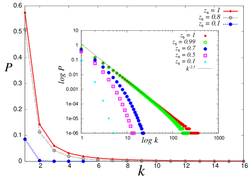
for $\alpha=1/2$. We show the $P(k)$ for several values of $z_{s}$ in Fig. 1.

Figure 1: The occupation probability of the Monkey class urn model with disorder. This figure was taken from our previous paper Inoue2008 .

From this figure, we find that before condensation, namely, for $z_{s}<1,\rho<\rho_{c}$, the occupation probability is given by

$$P(k)=\frac{(1-z_{s})\varepsilon_{0}}{\beta^{3/2}}k^{-3/2}{\rm e}^{-k\log(1/z_{s})}$$ (10)

On the other hand, after condensation, that is, for $z_{s}=1,\rho\geq\rho_{c}$, we have

$$P(k)=\frac{3\varepsilon_{0}\Gamma(3/2)}{2\beta^{3/2}}k^{-5/2}+\frac{1}{N}\delta(k-k_{*})$$ (11)

The important remarks here are the fact that the condensation is specified by the power-law behavior of the occupation probability and for the case of without disorder, namely, for $D(\varepsilon)=\delta(\varepsilon-\varepsilon_{0})$, the power-law behavior disappears.

As we saw, the urn model with disorder exhibits a rich physical phenomena such as condensation, however, there is no explicit interaction between agents (balls and urns). Actually, when we consider the job-matching process, it is impossible to accept the assumption that there is no correlation between urns (companies), balls (students), or between urns and balls. Hence, we should use a different description of the system. In the next section, we use the so-called Potts model to describe the problem of human resource allocation.

3 Correlations: The Potts model descriptions

The basic model proposed here for this purpose is described by the so-called Potts spin glass model which is well-known in the research field of statistical physics. In the model, each Potts spin represents the action of each student, and it takes a discrete value (integer) corresponding to the company he/she applies for. The pairwise interaction term in the energy function describes cross-correlations between students, and it makes our previous model Chen ; Chen2 ; Chen3 more realistic. Obviously, labor science deals with empirical evidence in labor markets and it is important for us to look for the so-called ‘stylized facts’ which have been discussed mainly in financial markets Cont ; Anirban . We also should reproduce the findings from data-driven models to forecast the market’s behavior.

In following, we show the limited results. Here we consider the system of labor market having $N$ students and $K$ companies. To make the problem mathematically tractable, we construct the energy (Hamiltonian) to include three distinct effects on the students’ behavior:

$$H(\bm{\sigma}_{t})=-\frac{J}{N}\sum_{ij}c_{ij}\,\delta_{\sigma_{i}^{(t)},\sigma_{j}^{(t)}}-\gamma\sum_{i=1}^{N}\sum_{k=0}^{K-1}\epsilon_{k}\,\delta_{k,\sigma_{i}^{(t)}}+\sum_{i=1}^{N}\sum_{k=0}^{K-1}\beta_{k}\left|v_{k}^{*}-v_{k}(t-1)\right|\delta_{k,\sigma_{i}^{(t)}},$$ (12)

where $\delta_{a,b}$ denotes a Kronecker’s delta and a Potts spin $\sigma_{i}^{(t)}$ stands for the company which student $i$ post his application letter to at stage (or time) $t$, namely,

$$\sigma_{i}^{(t)}\in\{0,\cdots,K-1\},\,\,\,i=1,\cdots,N.$$ (13)

Therefore, the first term in the above equation (12) denotes a collective effect, the second corresponds to the ranking of companies and the third term is a market history. In order to include the cross-correlations between students, we describe the system by using the Potts spin glass (see the ‘quenched’ random variables $c_{ij}$ in (12)) as a generalization of the Sherrington-Kirkpatrick model, which is well-known as an exactly solvable model for spin glass so far. The overall energy function of probabilistic labor market is written explicitly by (12). $c_{ij}$ is an adjacency matrix standing for the ‘interpersonal relationship’ of students, and one can choose an arbitrary form, say

$$c_{ij}=\left\{\begin{array}[]{cl}c&(\mbox{students $i,j$ are `friendly'})\\ 0&(\mbox{students $i,j$ are `independent'})\\ -c&(\mbox{students $i,j$ are `anti-friendly'})\end{array}\right.$$ (14)

for $c>0$ and the ranking of the company $k$ is defined by $\epsilon_{k}$ (see e.g. Chen2 for the detail).

Before investigating some specific cases below, we shall first provide a general setup. Let us introduce a microscopic variable, which represents the decision making of companies for a student as

$$\xi_{i}^{(t)}=\left\{\begin{array}[]{cl}1&(\mbox{student $i$ receives an acceptance at stage $t$})\\ 0&(\mbox{student $i$ is rejected at stage $t$})\end{array}\right.$$ (15)

Then, the conditional probability is given by

$$P(\xi_{i}^{(t)}|\sigma_{i}^{(t)})=1-A(\sigma_{i}^{(t)})-(1-2A(\sigma_{i}^{(t)}))\xi_{i}^{(t)}$$ (16)

with the acceptance ratio

$$A(\sigma_{i}^{(t)})\equiv\sum_{k=0}^{K-1}\delta_{k,\sigma_{i}^{(t)}}\Theta(v_{k}^{*}-v_{k}(t))+\sum_{k=0}^{K-1}\delta_{k,\sigma_{i}^{(t)}}\,\frac{v_{k}^{*}}{v_{k}(t)}\,\Theta(v_{k}(t)-v_{k}^{*}),$$ (17)

where $v_{k}^{*}(=1/K,\,\mbox{for simplicity in this paper})$ and $v_{k}(t)$ denote the quota and actual number of applicants to the company $k$ per student at stage $t$, respectively. $\Theta(\cdots)$ is a conventional step function. Hence, when we assume that selecting procedure by companies is independent of students, we immediately have

$$P(\bm{\xi}_{t}|\bm{\sigma}_{t}) = \prod_{i=1}^{N}P(\xi_{1}^{(t)}|\sigma_{1}^{(t)})\cdots P(\xi_{N}^{(t)}|\sigma_{N}^{(t)})$$ (18)

$$= {\exp}\left[\sum_{i=1}^{N}\log\left\{1-A(\sigma_{i}^{(t)})-(1-2A(\sigma_{i}^{(t)}))\xi_{i}\right\}\right].$$

Thus, we calculate the joint probability $P(\bm{\xi}_{t},\bm{\sigma}_{t})$ by means of $P(\bm{\xi}_{t}|\bm{\sigma}_{t})P(\bm{\sigma}_{t})$ as

$$P(\bm{\xi}_{t},\bm{\sigma}_{t}) = P(\bm{\xi}_{t}|\bm{\sigma}_{t})P(\bm{\sigma}_{t})$$

$$= \frac{{\exp}\left[\sum_{i=1}^{N}\log\left\{1-A(\sigma_{i}^{(t)})-(1-2A(\sigma_{i}^{(t)}))\xi_{i}^{(t)}\right\}-H(\bm{\sigma}_{t})\right]}{\sum_{\bm{\xi}_{t},\bm{\sigma}_{t}}{\exp}\left[\sum_{i=1}^{N}\log\left\{1-A(s_{i}^{(t)})-(1-2A(s_{i}^{(t)}))\xi_{i}^{(t)}\right\}-H(\bm{\sigma}_{t})\right]}$$

where we assumed that the $P(\bm{\sigma}_{t})$ obeys a Gibbs-Boltzmann distribution for the energy function (12) as $\sim{\rm e}^{-H(\bm{\sigma}_{t})}$.

Therefore, the employment rate as a macroscopic quantity:

$$1-U(t)=\frac{1}{N}\sum_{i=1}^{N}\xi_{i}^{(t)}$$ (20)

is evaluated as an average over the joint probability $P(\bm{\xi}_{t},\bm{\sigma}_{t})$, and in the thermodynamic limit $N\to\infty$, it leads to

$$1-U(t) = \frac{\sum_{\bm{\xi}_{t},\bm{\sigma}_{t}}\xi_{i}\,{\exp}\left[\sum_{i=1}^{N}\log\left\{1-A(\sigma_{i}^{(t)})-(1-2A(\sigma_{i}^{(t)}))\xi_{i}^{(t)}\right\}-H(\bm{\sigma}_{t})\right]}{\sum_{\bm{\xi}_{t},\bm{\sigma}_{t}}{\exp}\left[\sum_{i=1}^{N}\log\left\{1-A(\sigma_{i}^{(t)})-(1-2A(\sigma_{i}^{(t)}))\xi_{i}^{(t)}\right\}-H(\bm{\sigma}_{t})\right]}$$ (21)

$$= \frac{\sum_{\bm{\sigma}_{t}}A(\sigma_{i}^{(t)})\,{\exp}[-H(\bm{\sigma}_{t})]}{\sum_{\bm{\sigma}_{t}}{\exp}[-H(\bm{\sigma}_{t})]}\equiv\langle A(\sigma_{i}^{(t)})\rangle,$$

where we defined the bracket:

$$\langle\cdots\rangle\equiv\frac{\sum_{\bm{\sigma}_{t}}(\cdots)\,{\exp}[-H(\bm{\sigma}_{t})]}{\sum_{\bm{\sigma}_{t}}{\exp}[-H(\bm{\sigma}_{t})]}.$$ (22)

From the resulting expression (22), we are confirmed that the employment rate $1-U(t)$ is given by an average of the acceptance ratio (17) over the Gibbs-Boltzmann distribution for the energy function (12). Using the above general formula, we shall calculate the employment rate exactly for several limited cases.

4 The results

In following, we show our several limited contributions. Before we show our main result, we shall give a relationship between the Potts modeling and our previous studies Chen ; Chen2 ; Chen3 which are obtained by simply setting $J=0$ in (12).

4.1 For the case of $J=0$

We first consider the case of $J=0$. For this case, the energy function (12) is completely ‘decoupled’ as follows.

$$H(\bm{\sigma}_{t}) = \sum_{i}H_{i},$$ (23)

$$H_{i} = -\sum_{k=0}^{K-1}\{\gamma\epsilon_{k}-\beta|v_{k}^{*}-v_{k}(t-1)|\}\delta_{\sigma_{i}^{(t)},k}$$ (24)

where we set $\beta_{k}=\beta\,(\forall_{k})$ for simplicity. Hence, the $v_{k}(t)$ is evaluated in terms of the definition (22) as

$$v_{k}(t)\equiv\lim_{N\to\infty}\frac{1}{N}\sum_{i=1}^{N}\delta_{\sigma_{i}^{(t)},k}=\left\langle\delta_{\sigma_{i}^{(t)},k}\right\rangle=\frac{{\exp}[-\gamma\epsilon_{k}+\beta|v_{k}^{*}-v_{k}(t-1)|]}{\sum_{k=0}^{K-1}{\exp}[-\gamma\epsilon_{k}+\beta|v_{k}^{*}-v_{k}(t-1)|]}$$ (25)

and from the expression of employment rate (21), we have

$$1-U(t)=\frac{\sum_{k=0}^{K-1}\left\{\frac{v_{k}^{*}}{v_{k}(t)}+\left(1-\frac{v_{k}^{*}}{v_{k}(t)}\right)\Theta(v_{k}^{*}-v_{k}(t))\right\}{\exp}[-\gamma\epsilon_{k}+\beta|v_{k}^{*}-v_{k}(t-1)|]}{\sum_{k=0}^{K-1}{\exp}[-\gamma\epsilon_{k}+\beta|v_{k}^{*}-v_{k}(t-1)|]}.$$ (26)

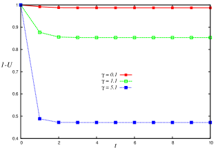
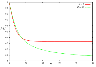
By solving the non-linear equation (25) recursively and substituting the solution $v_{k}(t)$ into (26), we obtain the time-dependence of the employment rate $1-U(t)$. In Fig. 2, we plot the time-dependence of the employment rate for the case of $K=3$ (left) and the $\gamma$-dependence of the employment rate at the steady state at $t=10$ for $K=3$ and $K=50$ (right). We set the job-offer ratio defined in Chen ; Chen2 ; Chen3 as $\alpha=1$. The ranking factor is also selected by

$$\epsilon_{k}=1+\frac{k}{K}.$$ (27)

We here assumed that each agent posts only a single application letter to the market, namely, $a=1$ in the definition of the previous studies Chen ; Chen2 ; Chen3 . It should be important for us to remind that the above equation (25) is exactly the same as the update rule for the aggregation probability $P_{k}(t)$ in the reference Chen . However, when we restrict ourselves to the case of $\alpha=a=1$, one can obtain the time-dependence of the employment rate exactly by (26). This is an advantage of this approach. It also should be noted that from the relationship:

$$U=\alpha\Omega+1-\alpha$$ (28)

(see Chen for the derivation), we have $U=\Omega$, namely, the unemployment rate is exactly the same as the labor shortage ratio for $\alpha=1$.

Figure 2: The time-dependence of the employment rate for the case of $K=3$ (left) and the $\gamma$-dependence of the employment rate at the steady state at $t=10$ for $K=3$ and $K=50$ (right). We set the job-offer ratio defined in Chen ; Chen2 ; Chen3 as $\alpha=1$ and assume that each agent posts only a single application letter to the market, namely, $a=1$ in the definition of the previous studies Chen ; Chen2 ; Chen3 .

It is important for us to notice that the aggregation probability of the system $P(\bm{\sigma}_{t})$ is rewritten in terms of $P_{k}(t)$ in the references Chen ; Chen2 ; Chen3 as

$$P(\bm{\sigma}_{t})=\left\{\prod_{k=1}^{K}P_{k}(t)\right\}^{N}$$ (29)

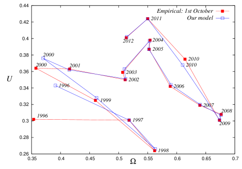
with $P_{k}(t)=v_{k}(t)$ (see (25)) even for $\alpha\neq 1$. For this case, the system parameters are only $\gamma$ and $\beta$, and these unknown parameters are easily calibrated from the empirical data Chen3 . As the result, we obtained $U$-$\Omega$ curve using (28) for the past 17 years in Japanese labor market for university graduates.

Figure 3: The empirical and theoretical $U$-$\Omega$ curves. We clearly find that the large $\gamma$ apparently pushes the $U$-$\Omega$ curve toward the upper right direction where the global mismatch between the students and companies is large. The picture was taken from our previous study Chen3 .

We plot the resulting and $U$-$\Omega$ curve in Fig. 3. The gap between the theoretical and empirical curves comes from the uncertainties in the calibration of average number of application letters $a$. In this figure, we simply chose the value as $a=10$ in our calculations.

4.2 The case of $J\neq 0$

We next consider the case of $J\neq 0$. Then, we should note that some ‘chiral representation’ of the energy function (12) by means of the chiral Potts spin Nishimori ; Carlucci (Note: ‘$i$’ appearing in ‘$2\pi i$’ below is an imaginary unit):

$$\lambda_{i}={\exp}\left(\frac{2\pi i}{K}\sigma_{i}^{(t)}\right),\,\sigma_{i}^{(t)}=0,\cdots,K-1$$ (30)

enables us to obtain some analytical insights into our labor markets.

The case of $\gamma=\beta=0$: Without ranking and market history

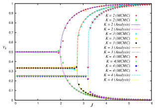
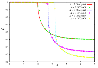
As a preliminary, we show the employment rate $1-U$ as a function of $J(>0)$ for the simplest case $\gamma=\beta=0$ and $c_{ij}=1\,(\forall_{ij})$ in Fig. 4 (right), and the actual number of applicants the company $k$ obtains in Fig. 4 (left). We should keep in mind that for this simplest case with local energy

$$H_{ij}\equiv-J\delta_{\sigma_{i},\sigma_{j}}=-\frac{J}{K}\sum_{r=0}^{K-1}\lambda_{i}^{r}\lambda_{j}^{K-r}=-\frac{J}{K}\left\{1+\sum_{r=1}^{K-1}\lambda_{i}^{r}\lambda_{j}^{K-r}\right\}$$ (31)

under the transformation (30) leading to the total energy $H(\bm{\sigma})\equiv\sum_{ij}H_{ij}$, by evaluating the partition function:

$$Z=\sum_{\bm{\sigma}}{\exp}\left[\frac{J}{NK}\sum_{r=1}^{K-1}\sum_{ij}\cos\frac{2\pi r(\sigma_{i}-\sigma_{j})}{K}\right]$$ (32)

in the limit of $N\to\infty$, one can obtain the employment rate $1-U=\langle A(\bm{\sigma})\rangle$ (see also equation (21)) exactly as

$$1-U = \frac{\sum_{\bm{\sigma}}A(\bm{\sigma})\,{\exp}[-H(\bm{\sigma)}]}{\sum_{\bm{\sigma}}{\exp}[-H(\bm{\sigma})]}$$

$$= \frac{\left\{\frac{v_{0}^{*}}{v_{0}}+\left(1-\frac{v_{0}^{*}}{v_{0}}\right)\Theta(v_{0}^{*}-v_{0})\right\}}{1+(K-1){\rm e}^{-\frac{Jx}{K-1}}}+\frac{(K-1)\left\{\frac{v_{k}^{*}}{v_{k}}+\left(1-\frac{v_{k}^{*}}{v_{k}}\right)\Theta(v_{k}^{*}-v_{k})\right\}{\rm e}^{-\frac{Jx}{K-1}}}{1+(K-1){\rm e}^{-\frac{Jx}{K-1}}}$$

with

$$v_{k}\equiv\lim_{N\to\infty}\frac{1}{N}\sum_{i=1}^{N}\delta_{\sigma_{i},k}=\left\langle\delta_{\sigma,k}\right\rangle=\frac{\delta_{0,k}+\sum_{\sigma=1}^{K-1}\delta_{\sigma,k}\,{\rm e}^{-\frac{Jx}{K-1}}}{1+(K-1)\,{\rm e}^{-\frac{Jx}{K-1}}},\,\,\,k=0,\cdots,K-1,$$ (34)

where an order parameter $x$ is determined as a solution of the following non-linear equation:

$$x=(K-1)\left(\frac{1-{\rm e}^{-\frac{J}{K-1}x}}{1+(K-1){\rm e}^{-\frac{J}{K-1}x}}\right).$$ (35)

It should be noted that the above $x$ is given by the extremum of the free energy density:

$$f=-\frac{Jx^{2}}{K(K-1)}+\log\sum_{\sigma=0}^{K-1}{\exp}\left[\frac{Jx}{K(K-1)}\sum_{r=1}^{K-1}\cos\left(\frac{2\pi r}{K}\sigma\right)\right].$$ (36)

The acceptance ratio $A(\bm{\sigma})$ is now given by

$$A(\bm{\sigma})\equiv\sum_{i=1}^{N}A(\sigma_{i})=\sum_{i=1}^{N}\sum_{k=0}^{K-1}\delta_{\sigma_{i},k}\left\{\frac{v_{k}^{*}}{v_{k}}+\left(1-\frac{v_{k}^{*}}{v_{k}}\right)\Theta(v_{k}^{*}-v_{k})\right\},$$ (37)

and we omitted the time $t$-dependence in the above expressions because the system is no longer dependent on the market history, namely $v_{k}(t-1)$, for the choice of $\beta=\gamma=0$ in the energy function (12).

In Fig. 4, we easily find that phase transitions take place when the strength of ‘cooperation’ $J$ increases beyond the critical point $J_{\rm c}$. Namely, for weak $J$ regime, ‘random search’ by students is a good strategy to realize the perfect employment state ($1-U=1$), however, once $J$ increases beyond the critical point, the perfect state is no longer stable and system suddenly goes into the extremely worse employment phase for $K\geq 3$ (first order phase transition). The critical point of the second order phase transition for $K=2$ is easily obtained by expanding (35) around $x=0$ as

$$x=\frac{1-{\rm e}^{-Jx}}{1+{\rm e}^{-Jx}}\simeq Jx/2$$ (38)

and this reads $J_{\rm c}=2$. For the first order phase transition, we numerically obtain the critical values, for instance, we have $J_{\rm c}=2.73$ for $K=3$ and $J_{\rm c}=3.21$ for $K=4$. As the number $K$ is quite large far beyond $K=3$ in real labor markets, hence the above finding for the discontinuous transition might be useful for discussing a mismatch between students and companies, which is a serious issue in recent Japanese labor markets (see the reference Chen3 ).

We also carried out computer simulations to examine the efficiency of the model. We should mention that the analytic results (lines) and the corresponding Monte Carlo simulations (dots) with finite system size $N=1000$ are in an excellent agreement in the figures. This preliminary result is a justification for us to conform that one can make a mathematically rigorous platform to investigate the labor market along this direction.

Figure 4: The actual number of applicants $v_{k}$ (left) and employment rate $1-U$ (right) as a function of the strength of cooperation $J$. We find that the system undergoes a phase transition at the critical point. The transition is the second order for $K=2$, whereas it is the first order for $K\geq 3$. These critical points are given by $J_{\rm c}=2$ for $K=2$, $J_{\rm c}=2.73$ for $K=3$ and $J_{\rm c}=3.21$ for $K=4$. We should mention that the analytic results (lines) and the corresponding Monte Carlo simulations (MCMC) with the finite number of students $N=1000$ (dots) are in an excellent agreement. We should notice that perfect employment phase is a ‘disordered phase’, whereas the poor employment phase corresponds to an ‘ordered phase’ in the literature of order-disorder phase transition. For large strength of cooperation $J$, as a company occupies all applications up to the quota, $\lim_{J\to\infty}(1-U)=v_{k}^{*}=1/K$ (the quota per student) is satisfied.

We next consider the case of $\beta,\gamma\neq 0$.

Ranking effects

For the case of $\gamma\neq 0,\beta_{k}=0\,(\forall_{k})$, the saddle point equation is given by the following two-dimensional vector form:

$$(x_{r},y_{r})=\langle\bm{u}_{r}(s)\rangle_{*}=\left(\left\langle\cos\frac{2\pi r}{K}s\right\rangle_{*},\left\langle\sin\frac{2\pi r}{K}s\right\rangle_{*}\right),\,\,\,r=0,\cdots,K-1$$ (39)

where we defined the bracket $\langle\cdots\rangle_{*}$ as

$$\langle\cdots\rangle_{*}\equiv\frac{\sum_{s=0}^{K-1}(\cdots)\,{\exp}[\psi_{r}(s:\{x_{r}\},\{y_{r}\})]}{\sum_{s=0}^{K-1}{\exp}[\psi_{r}(s:\{x_{r}\},\{y_{r}\})]},$$ (40)

$$\psi_{r}(s:\{x_{r}\},\{y_{r}\})\equiv\sum_{r=0}^{K-1}\bm{X}_{r}\cdot\bm{u}_{r}(s)$$ (41)

with the following two vectors:

$$\bm{X}_{r} = \left(\frac{J}{K}x_{r}+\frac{\gamma}{K}\sum_{k=0}^{K-1}\epsilon_{k}\cos\frac{2\pi r}{K}k,\frac{J}{K}y_{r}+\frac{\gamma}{K}\sum_{k=0}^{K-1}\epsilon_{k}\sin\frac{2\pi r}{K}k\right)$$ (42)

$$\bm{u}_{r}(s) = \left(\cos\frac{2\pi r}{K}s,\sin\frac{2\pi r}{K}s\right).$$ (43)

From the energy function (12) and the above formula, we should notice that the ranking factor $\epsilon_{k}$ is regarded as a ‘state-dependent field’ affecting each spin and the symmetry in the ‘perfect employment phase’ for small $J$ (see Fig. 4 (right)) might be broken by these unbiased effects. We also should keep in mind that for the case of $\gamma=0$ or $\epsilon_{k}=\epsilon\,\,(\forall_{k})$, we find that the equation (39) possesses the solution of the type: $x_{0},\cdots,x_{K-1}\neq 0,\,y_{0}=\cdots=y_{K-1}=0$. It should be also bear in mind that $K=2$ is rather a special case and the solution of the above type is obtained simply as

$$x_{0}=1,\,x\equiv x_{1}=\frac{1-{\rm e}^{-Jx+\gamma(\epsilon_{1}-\epsilon_{0})}}{1+{\rm e}^{-Jx+\gamma(\epsilon_{1}-\epsilon_{0})}},\,\,y_{0}=y_{1}=0.$$ (44)

However, for general case, we must deal with two-dimensional vectors $(x_{r},y_{y}),\,r=0,\cdots,K-1$ with each non-zero component $x_{r},y_{r}\neq 0$ to specify the equilibrium properties of the system.

For the solution $(x_{r},y_{r}),\,r=0,\cdots,K-1$, we obtain the order parameters and employment rate as

$$v_{r} = \langle\delta_{r,s}\rangle_{*}$$ (45)

$$1-U = \langle A(s)\rangle_{*},\,\,\,r=0,\cdots,K-1.$$ (46)

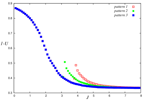
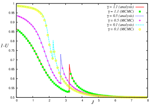
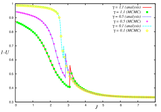
In Fig. 5, we plot the $J$-dependence of the employment rate for $K=2$ (left) and $K=3$ (right). From this figure, we find that the employment rate decreases monotonically, however, within intermediate range of $J$, the $1-U$ behaves discontinuously. We should notice that in this regime, the ‘ergodicity’ of the system might be broken because the realized value of $1-U$ by Monte Carlo simulation is strongly dependent on the choice of initial configuration (pattern) of Potts spins.

Figure 5: The strength of cooperation $J$-dependence of the employment rate for the case of $\gamma\neq 0,\beta_{k}=0\,(\forall_{k})$. We plot the case of $K=2$ (left) and $K=3$ (right). We find that the phase transition as shown in Fig. 4 disappears, however, the ergodicity breaking phase appears within intermediate range of $J$. We are conformed that $\lim_{J\to\infty}(1-U)=1/K$ is satisfied even for this case. The simulations (MCMC) are carried out for the system of size $N=1000$.

To see the result more explicitly, we should draw our attention to the initial condition dependence of the $J$-$(1-U)$ curve. Actually, here we carry out Monte Carlo simulation to examine the initial configuration dependence of the $1-U$ numerically and show the results in Fig. 6. From this figure, we confirm that the value of the $1-U$ depends on the initial configuration of the Potts spins although the $1-U$ is independent of the initial condition for $J<3$ and $J\gg 1$. In this plot, we chose the two distinct initial conditions so as to make the gap of order parameters $\mathcal{O}(1)$ object, that is,

$$\Delta x_{r}(\equiv x_{r}^{(\rm a)}-x_{r}^{({\rm b})}),\Delta y_{r}(\equiv y_{r}^{(\rm a)}-y_{r}^{({\rm b})})\sim\mathcal{O}(1)$$ (47)

for $r=0,\cdots,K-1$.

Figure 6: The initial configuration dependence of the $1-U$. We set $K=3,\gamma=1.1$ and choose three distinct initial configurations for Monte Carlo simulations. We find that $1-U$ is strongly dependent on the initial condition (‘pattern $1\sim 3$’) within intermediate range of $J$. In this plot, we chose the two distinct initial conditions so as to make the gap of order parameters $\mathcal{O}(1)$ object, that is, $\Delta x_{r}(\equiv x_{r}^{(\rm a)}-x_{r}^{({\rm b})}),\Delta y_{r}(\equiv y_{r}^{(\rm a)}-y_{r}^{({\rm b})})\sim\mathcal{O}(1)$ for $r=0,\cdots,K-1$ $({\rm a,b}=\{\mbox{\tt pattern 1,pattern 2, pattern 3}\})$.

It might be important for us to investigate the basin of attraction for the matching dynamics analytically as in the reference Inoue , however, it is far beyond the scope of the current paper and it should be addressed our future study.

Market history effects

We next consider the case of $\beta_{k}\neq 0\,(\forall_{k})$. For this case, we should replace the $\bm{X}_{r}$ in the saddle point equation (39) by

$$\bm{X}_{r} = {\Biggr{(}}\frac{J}{K}x_{r}+\frac{1}{K}\sum_{k=0}^{K-1}(\gamma\epsilon_{k}-\beta_{k}|v_{k}^{*}-v_{k}(t-1)|)\cos\frac{2\pi r}{K}k,$$ (48)

$$\frac{J}{K}y_{r}+\frac{1}{K}\sum_{k=0}^{K-1}(\gamma\epsilon_{k}-\beta_{k}|v_{k}^{*}-v_{k}(t-1)|)\sin\frac{2\pi r}{K}k{\Biggr{)}}.$$

It should be noticed that the $v_{k}$ at the previous stage $t-1$ is regarded as an ‘external field’ which affects the spin system at the current stage $t$. Hence, by substituting $v_{k}(0)$ as an initial state into the equation (39) with (48), we can solve the equation with respect to $v_{k}(1)$. By repeating the procedures, we obtain the ‘time series’ as $v_{k}(0)\to v_{k}(1)\to\cdots v_{k}(t)\to$ for all $k$ and $1-U(t)$ as a function of $t$.

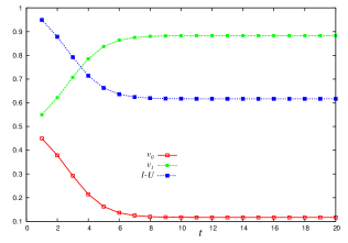
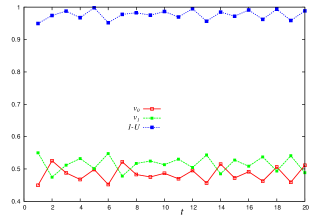
Figure 7: The time (stage) dependence of the employment rate $1-U$ for the case of $K=2,J=1,\gamma=0.1$ and $(\beta_{1},\beta_{0})=(1,4)$ (left) and $(\beta_{1},\beta_{0})=(4,1)$ (right). The ‘zigzag behavior’ in $v_{k}(t)$ is observed for $(\beta_{1},\beta_{0})=(4,1)$.

In Fig. 7, we plot the time (stage) dependence of the employment rate $1-U$ for the case of $K=2,J=1,\gamma=0.1$ and $(\beta_{1},\beta_{0})=(1,4)$ (left) and $(\beta_{1},\beta_{0})=(4,1)$ (right). From this figure, we find that the larger weight of the market history effect for the highest ranking company $\beta_{1}$ in comparison with $\beta_{0}$ induces the periodical change of the order for $v_{1},v_{0}$ due to the negative feedback (a sort of ‘minority game’ Minority for the students). Namely, from the ranking gap $\epsilon_{1}-\epsilon_{0}=1/2$ for $K=2$, the company ‘1’ attracts a lot of applications at time $t$ even for a relatively small strength of the preference $\gamma=0.1$. However, at the next stage, the ability of the aggregation for the company ‘1’ remarkably decreases due to the large $\beta_{1}$. As the result, the inequality $v_{1}>v_{0}$ is reversed as $v_{0}>v_{1}$, and the company ‘0’ obtains much more applications than the company ‘1’ at this stage. After several time steps, the amount of $\beta_{1}|v_{1}^{*}-v_{1}(t-1)|$ becomes small enough to turn on the switch of the preference for the high ranking company ‘1’, and eventually the inequality $v_{1}>v_{0}$ should be recovered again. The ‘zigzag behavior’ due to the above feedback mechanism in $v_{k}(t)$ is actually observed in Fig. 7 (right). On the other hand, when the strength of the history effect $\beta_{0}$ for the lower ranking company is larger than that of the higher ranking company $\beta_{1}$, the zigzag behavior disappears and $v_{0},v_{1}$ converge monotonically to the steady states reflecting the ranking $\epsilon_{0}<\epsilon_{1}$.

5 Summary and discussion

In this paper, we proposed a mathematical toy model, the so-called chiral Potts model to investigate the job-matching process in Japanese labor markets for university graduates and investigated the behavior analytically. We found several characteristic properties in the system. Let us summarize them below. For the case without ranking effect and market history, we observed that the system undergoes fist order phase transition for $K\geq 3$ by changing the strength of cooperation $J(>0)$. When we take into account the ranking effect without market history, the ergodicity breaking region in $J$ appears. The market history affects on the dynamics of actual number of applicants to each company $v_{k}(t)$ to exhibit ‘zig-zag’ behavior.

We would like to stress that the situation and our modeling are applicable to the other type of resource allocation (utilization) such as the so-called Kolkata Paise Restaurant (KPR) problem KPR .

5.1 Inverse problem of the Potts model

However, from the view point of empirical science, in this model system, the cross-correlations (the adjacent matrix) between students and companies are unknown and not yet specified. Hence, we should estimate these elements by using appropriate empirical data sets. For instance, if we obtain the ‘empirical correlation’ $\langle\delta_{\sigma_{i},\sigma_{j}}\rangle_{\rm emprical}$ from the data, we can determine $c_{ij}$ so as to satisfy the following relationship:

$$\langle\delta_{\sigma_{i},\sigma_{j}}\rangle = \frac{\partial}{\partial c_{ij}}\log\sum_{\bm{\sigma}}{\exp}[-H(\bm{\sigma}:\{c_{ij}\})]$$ (49)

$$= \frac{\sum_{\bm{\sigma}}\delta_{\sigma_{i},\sigma_{j}}{\exp}[-H(\bm{\sigma}:\{c_{ij}\})]}{\sum_{\bm{\sigma}}{\exp}[-H(\bm{\sigma}:\{c_{ij}\})]}=\langle\delta_{\sigma_{i},\sigma_{j}}\rangle_{\rm emprical}$$

where $\langle\delta_{\sigma_{i},\sigma_{j}}\rangle_{\rm emprical}$ might be evaluated empirically as a time-average by

$$\langle\delta_{\sigma_{i},\sigma_{j}}\rangle_{\rm emprical}=(1/\tau)\sum_{t=t_{0}}^{\tau+t_{0}}\delta_{\sigma_{i}^{(t)},\sigma_{j}^{(t)}}.$$ (50)

We might also use the EM (Expectation and Maximization)-type algorithm Inoue2002 to infer the interactions. Those extensive studies in this directions (the ‘inverse Potts problem’) including collecting the empirical data are now working in progress.

5.2 Learning of valuation basis of companies

In this paper, we did not take into account the details of valuation process by companies so far. In our modeling, we assumed that they randomly select suitable students from the candidates up to their quota. This is because the valuation basis is unfortunately not opened for the public and it is somewhat ‘black box’ for students. However, recently, several web sites Rikunabi ; Mynabi for supporting job hunting might collect a huge number of information about students as their ‘scores’ of aptitude test.

Hence, we might have a $N$-dimensional vector, each of whose component represents a score for a given question, for each student $l=1,\cdots,L$ as

$$\bm{x}^{(l)}=(x_{1}^{(l)},x_{2}^{(l)},\cdots,x_{N}^{(l)})$$ (51)

Then, we assume that each company $\mu=1,\cdots,K$ possesses their own valuation basis (weight) as a $N$-dimensional vector $\bm{a}_{\mu}=(a_{\mu 1},\cdots,a_{\mu N})$ and the score of student $l$ evaluated by the company $\mu=1,\cdots,K$ is given by

$$y_{\mu}^{(l)}=a_{\mu 1}x_{1}^{(l)}+a_{\mu 2}x_{2}^{(l)}+\cdots+a_{\mu N}x_{N}^{(l)},\,\,\mu=1,\cdots,K.$$ (52)

It is naturally accepted that the company $\mu$ selects the students who are the $v_{\mu}^{*}$-top score candidates. Therefore, For a given threshold $\theta_{\mu}$, the decision by companies is given by

$$\hat{y}_{\mu}^{(l)}=\Theta(y_{\mu}^{(l)}-\theta_{\mu})=\left\{\begin{array}[]{cl}1&(\mbox{accept})\\ 0&(\mbox{reject})\end{array}\right.$$ (53)

where $\Theta(\cdots)$ is a unit step function.

Thus, for $L$ students and $K$ companies, the situation is determined by the following linear equation:

$$\left(\begin{array}[]{c}y_{1}^{(l)}\\ \cdot\\ \cdot\\ \cdot\\ y_{M}^{(l)}\end{array}\right)=\left(\begin{array}[]{ccccc}a_{11}&\cdots&\cdots&\cdots&a_{1N}\\ \cdots&\cdots&\cdots&\cdots&\cdots\\ \cdots&\cdots&\cdots&\cdots&\cdots\\ \cdots&\cdots&\cdots&\cdots&\cdots\\ a_{M1}&\cdots&\cdots&\cdots&a_{MN}\end{array}\right)\left(\begin{array}[]{c}x_{1}^{(l)}\\ \cdot\\ \cdot\\ \cdot\\ \cdot\\ \cdot\\ x_{N}^{(l)}\end{array}\right),\,\,\,l=1,\cdots,L$$ (54)

namely,

$$\bm{y}^{(l)}=\bm{A}\bm{x}^{(l)},\,\,l=1,\cdots,L.$$ (55)

When we have enough number of data sets $(\bm{y}^{(l)},\bm{x}^{(l)}),l=1,\cdots,L$, one might estimate the valuation base $\bm{A}$ by using suitable learning algorithm. When we notice that the above problem is described by ‘learning of a linear perceptron’, one might introduce the following cost function:

$$E=\frac{1}{2LM}\sum_{l=1}^{L}\sum_{\mu=1}^{M}\delta_{s_{\mu}^{(l)},1}\left\{y_{\mu}^{(l)}-\sum_{i=1}^{N}a_{\mu i}x_{i}^{(l)}\right\}^{2}$$ (56)

where we defined $\delta_{a,b}$ as Kroneker’s delta and

$$s_{\mu}^{(l)}=\left\{\begin{array}[]{cl}1&(\mbox{student $l$ sends an application letter to company $\mu$})\\ 0&(\mbox{otherwise})\end{array}\right.$$ (57)

Then, we construct the learning equation as

$$\frac{da_{\mu k}}{dt}=-\eta\frac{\partial E}{\partial a_{\mu k}}=\frac{\eta}{LM}\sum_{l=1}^{L}\delta_{s_{\mu}^{(l)},1}\left\{y_{\mu}^{(l)}-\sum_{i=1}^{N}a_{\mu i}x_{i}^{(l)}\right\}x_{k}^{(l)}$$ (58)

for $\mu=1,\cdots,M,k=1,\cdots,N$.

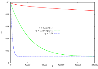
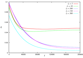
We show an example of the learning dynamics through the error:

$$\epsilon(t)=\frac{1}{NM}\sum_{\mu=1}^{M}\sum_{k=1}^{N}(a_{\mu k}^{*}-a_{\mu k}(t))^{2},$$ (59)

where $a_{\mu k}^{*}$ denotes a ‘true weight’, for artificial data sets in Fig. 8.

Figure 8: Time-dependence of error $\epsilon(t)=(1/NM)\sum_{\mu=1}^{M}\sum_{k=1}^{N}(a_{\mu k}^{*}-a_{\mu k}(t))^{2}$ for the learning equation (58) using artificial data sets. We choose the learning rate as $\eta=0.01/\log(2+t)$. $N=M=10$.

Here we showed just an example of learning from artificial data sets for demonstration, however, it should be addressed as our future work to apply the learning algorithm to realistic situation using empirical data set collected from Rikunabi ; Mynabi or large-scale survey.

Finally, it would be important for us to mention that it could be treated as ‘dictionary learning’ Sakata when the vector $\bm{x}^{(l)},l=1,\cdots,L$ is ‘sparse’ in the context of compressive sensing Candes ; Kabashima ; Sompolinsky .

Acknowledgements

This work was financially supported by Grant-in-Aid for Scientific Research (C) of Japan Society for the Promotion of Science (JSPS) No. 2533027803 and Grant-in-Aid for Scientific Research on Innovative Area No. 2512001313. One of the authors (JI) thanks Hideaki Aoyama, Bikas K. Chakrabarti, Asim Ghosh, Siew Ann Cheong, Yoshi Fujiwara, Shigehiro Kato, Matteo Marsili and Subinay Dasgupta for fruitful discussion and useful comments. One of the authors (HC) was financially supported by Grant-in-Aid for the JSPS Research Fellowship for Young Scientists. We acknowledge organizers of International Conference on Emerging Trends in Applied Mathematics, in particular, Susmita Sarkar for warm hospitality during our stay in Kolkata and editing the conference proceedings.

References

• (1) M. Aokiand H. Yoshikawa, ‘Reconstructing Macroeconomics: A Perspective from Statistical Physics and Combinatorial Stochastic Processes’, Cambridge University Press (2006).
• (2) T. Boeri and J Van Ours, ‘The Economics of Imperfect Labor Markets’, Princeton University Press (2008).
• (3) G. Fagiolo, G. Dosi and R. Gabriele, ‘Matching, Bargaining, and wage setting in an evolutionary model of labor market and output dynamics’, Advances in Complex System 7, No.2, pp. 157-186 (2004).
• (4) R. Gabriele, ‘Labor Market Dynamics and Institution: An Evolutionary Approach’, Working Paper in Laboratory of Economics and Management Sant’Anna School of Advances Studies, Pisa, Italy (2002).
• (5) M. Neugart, ‘Complicated dynamics in a flow model of the labor market’, Journal of Economic Behavior and Optimization 53, pp. 193-213 (2004).
• (6) S. Lippman and J.J. McCall, ‘The Economics of Job Search: A Survey’, Economic Inquiry 14, pp. 155-188 (1976).
• (7) P. A. Diamond, ‘Aggregate Demand Management in Search Equilibrium’, Journal of Political Economy 90, pp. 881-894 (1982).
• (8) C.A. Pissarides, “Short-Run Equilibrium Dynamics of Unemployment Vacancies”, American Economic Review 75, pp. 676-690 (1985).
• (9) C. A. Pissarides C A, Equilibrium Unemployment Theory, MIT Press (2000).
• (10) H. Chen and J. Inoue, ‘Dynamics of probabilistic labor markets: statistical physics perspective’, Lecture Notes in Economics and Mathematical Systems 662, pp. 53-64, ‘Managing Market Complexity’, Springer (2012).
• (11) H. Chen and J. Inoue, ‘Statistical Mechanics of Labor Markets’, Econophysics of systemic risk and network dynamics, New Economic Windows 2013, Springer-Verlag (Milan-Italy), pp.157-171 (2012).
• (12) H. Chen and J. Inoue, ‘Learning curve for collective behavior of zero-intelligence agents in successive job-hunting processes with a diversity of Jaynes-Shannon’s MaxEnt principle’, Evolutionary and Institutional Economics Review 10, No. 1, pp. 55-80 (2013).
• (13) J. Inoue and J. Ohkubo, ‘Power-law behavior and condensation phenomena in disordered urn models’, Journal of Physics A: Mathematical and Theoretical 41, 324020 (14pp) (2008).
• (14) R. Cont, ‘Empirical properties of asset returns: stylized facts and statistical issues’, Quantitative Finance 1, pp. 223 (2001).
• (15) A. Chakraborti, Y. Fujiwara, A. Ghosh, J. Inoue and S. Sinha, ‘Econophysics: Physicists’ approaches to a few economic problems’, submitted to Journal of Economic Interaction and Coordination (2013).
• (16) H. Nishimori and M.J. Stephen, ‘Gauge-invariant frustrated Potts spin-glass’, Phys. Rev. B 27, pp. 5644 (1983).
• (17) D.M. Carlucci and J. Inoue, ‘Image restoration using the chiral Potts spin glass’, Phys. Rev. E 60, pp. 2547 (1999).
• (18) J. Inoue and D.M. Carlucci, ‘Image restoration using the Q-Ising spin glass’, Phys. Rev. E 64, 036121 (2001).
• (19) D. Challet, M. Marsili and Yi.-C. Zhang, ‘Minority Games’, Oxford University Press (2005).
• (20) A. S. Chakrabarti, B. K. Chakrabarti, A. Chatterjee, and M. Mitra, ‘The Kolkata Paise Restaurant Problem and Resource Utilization’, Physica A 388, pp. 2420 (2009).
• (21) J. Inoue and K. Tanaka, ‘Dynamics of maximum marginal likelihood hyperparameter estimation in image restoration: Gradient descent versus expectation and maximization algorithm’, Phys. Rev. E 65, 016125 (9pages) (2002).
• (22) http://www.rikunabi.com
• (23) http://job.mynavi.jp
• (24) A. Sakata and Y. Kabashima, ‘Statistical mechanics of Dictionary Learning’ Europhys. Lett. 103 28008 (2013).
• (25) E.J. Candes and T. Tao, ‘Decoding by linear programming IEEE Trans. Info. Theory 51, 4203 (2005).
• (26) Y. Kabashima, T. Wadayama and T. Tanaka, ‘A typical reconstruction limit for compressive sensing on Lpsubscript𝐿𝑝L_{p}-norm minimization’, J. Stat. Mech., L09003 (2009).
• (27) S. Ganguli and H. Sompolinsky, ‘Statistical mechanics of compressive sensing’, Phys. Rev. Lett. 104 188701 (2010).