Optimal Explicit Strong Stability Preserving Runge–Kutta Methods with High Linear Order and optimal Nonlinear Order

Abstract

High order spatial discretizations with monotonicity properties are often desirable for the solution of hyperbolic PDEs. These methods can advantageously be coupled with high order strong stability preserving time discretizations. The search for high order strong stability time-stepping methods with large allowable strong stability coefficient has been an active area of research over the last two decades. This research has shown that explicit SSP Runge–Kutta methods exist only up to fourth order. However, if we restrict ourselves to solving only linear autonomous problems, the order conditions simplify and this order barrier is lifted: explicit SSP Runge–Kutta methods of any linear order exist. These methods reduce to second order when applied to nonlinear problems. In the current work we aim to find explicit SSP Runge–Kutta methods with large allowable time-step, that feature high linear order and simultaneously have the optimal fourth order nonlinear order. These methods have strong stability coefficients that approach those of the linear methods as the number of stages and the linear order is increased. This work shows that when a high linear order method is desired, it may be still be worthwhile to use methods with higher nonlinear order.

1 Introduction

Explicit strong stability preserving (SSP) Runge–Kutta methods were developed for the time evolution of hyperbolic conservation laws $U_{t}+f(U)_{x}=0$, with discontinuous solutions [16, 15]. These works studied total variation diminishing (TVD) spatial discretizations that can handle discontinuities. The spatial discretizations used to approximate $f(U)_{x}$ were carefully designed so that when the resulting system of ODEs

$$u_{t}=F(u),$$ (1)

(where $u$ is a vector of approximations to $U$, $u_{j}\approx U(x_{j})$) is evolved in time using the forward Euler method, the solution at time $u^{n}$ satisfies a strong stability property of the form

$$\|u^{n}+\Delta tF(u^{n})\|\leq\|u^{n}\|$$ (2)

under a step size restriction

$$0\leq\Delta t\leq\Delta t_{\textup{FE}}.$$ (3)

The term $\|\cdot\|$ can represent, as it did in [16, 15] the total variation semi-norm, or indeed any other semi-norm, norm, or convex functional, as determined by the design of the spatial discretization. These spatial discretizations satisfy the strong stability property $\|u^{n+1}\|\leq\|u^{n}\|$ when coupled with the forward Euler time discretization, but in practice a higher order time integrator, that will still satisfy this property, is desired. To accomplish this, we attempt to re-write a higher order time discretization as a convex combination of forward Euler steps, so that any convex functional property that is satisfied by the forward Euler method will still be satisfied by the higher order time discretization.

An $s$-stage explicit Runge–Kutta method can be written in the form [16],

$$u^{(0)} = u^{n},$$

$$u^{(i)} = \sum_{j=0}^{i-1}\left(\alpha_{i,j}u^{(j)}+\Delta t\beta_{i,j}F(u^{(j)})\right),\;\;\;\;i=1,...,s$$ (4)

$$u^{n+1} = u^{(s)}.$$

If all the coefficients $\alpha_{i,j}$ and $\beta_{i,j}$ are non-negative, and a given $\alpha_{i,j}$ is zero only if its corresponding $\beta_{i,j}$ is zero, then each stage can be rearranged into a convex combination of forward Euler steps

$$\|u^{(i)}\| = \|\sum_{j=0}^{i-1}\left(\alpha_{i,j}u^{(j)}+\Delta t\beta_{i,j}F(u^{(j)})\right)\|$$

$$\leq \sum_{j=0}^{i-1}\alpha_{i,j}\,\left\|u^{(j)}+\Delta t\frac{\beta_{i,j}}{\alpha_{i,j}}F(u^{(j})\right\|$$

$$\leq \|u^{n}\|\;\;\;\;\forall\Delta t\leq\min_{i,j}\frac{\alpha_{i,j}}{\beta_{i,j}}\Delta t_{\textup{FE}},$$

where if any of the $\beta$’s are equal to zero, the corresponding ratio is considered infinite. The last inequality above follows from the strong stability conditions (2) and (3)

$$\left\|u^{(j)}+\Delta tF(u^{(j})\right\|\leq\left\|u^{(j)}\right\|\;\;\;\forall\Delta t\leq\Delta t_{\textup{FE}}$$

and the consistency condition $\sum_{j=0}^{i-1}\alpha_{i,j}=1$. From this we can conclude that whenever the explicit Runge–Kutta method can be decomposed into convex combinations of forward Euler steps, then any convex functional property (3) satisfied by forward Euler will be preserved by the higher-order time discretizations, perhaps under a different time-step restriction $\Delta t\leq\mathcal{C}\Delta t_{\textup{FE}}$ [15]. Thus, this type of decomposition where $\min_{i,j}\frac{\alpha_{i,j}}{\beta_{i,j}}>0$ is clearly a sufficient condition for strong stability preservation. It has also been shown [2, 13, 17] that this convex combination condition is necessary for strong stability preservation. If a method does not have a convex combination decomposition into forward Euler steps we can find some ODE with some initial condition such that the forward Euler condition is satisfied but the method does not satisfy the strong stability condition for any positive time-step [2]. Methods that can be decomposed like this with with $\mathcal{C}>0$ are called strong stability preserving (SSP), and the coefficient $\mathcal{C}$ is known as the SSP coefficient of the method.

SSP methods guarantee the strong stability of the numerical solution for any ODE and any convex functional provided only that the forward Euler condition (2) is satisfied under a time step (3). This is a very strong requirement that leads to severe restrictions on the allowable order of SSP methods, and on the size of the allowable time step $\Delta t\leq\mathcal{C}\Delta t_{\textup{FE}}.$ We seek high order SSP Runge–Kutta methods with the largest allowable time-step. The forward-Euler time step $\Delta t_{\textup{FE}}$ is a property of the spatial discretization method only, and so our aim in searching for time-stepping methods that preserve the strong stability property is to maximize the SSP coefficient $\mathcal{C}$ of the method. A more relevant quantity may be the total cost of the time evolution, which in our case translates into the allowable time step relative to the number of function evaluations at each time-step (typically the number of stages of a method). For this purpose we define the effective SSP coefficient $\mathcal{C}_{\textup{eff}}=\frac{\mathcal{C}}{s}$ where $s$ is the number of stages. This value allows us to compare the efficiency of explicit methods of a given order. It has been shown [2] that all explicit $s$-stage Runge–Kutta methods have an SSP bound $\mathcal{C}\leq s$, and therefore $\mathcal{C}_{\textup{eff}}=1$, but this upper bound is not always attained.

In [13, 14] it was shown that explicit SSP Runge–Kutta methods cannot exist for order $p>4$ However, in the special case where we consider only linear autonomous problems, explicit SSP Runge–Kutta methods exist for any linear order $p_{lin}$ [1]. The linear and nonlinear order conditions are equivalent up to and including order $p=2$, so in this work we consider explicit SSP Runge–Kutta methods that have nonlinear order $p=3$ and $p=4$, and have higher linear orders $p_{lin}>p$. In Section 2 we review the SSP properties of explicit Runge–Kutta methods and discuss the linear and nonlinear order conditions. Using these order conditions and optimization problem described in [6, 7, 11, 9], in Section 3 we describe the optimization code in MATLAB (based on [5]) used to find explicit Runge–Kutta methods that have $p_{lin}>p$ with optimal SSP coefficient. In Section 4 we list some of the new methods and their effective SSP coefficients, and in Section 5 we demonstrate the performance of these methods on a selection of test problems.

2 A review of explicit SSP Runge–Kutta methods

Strong stability preserving methods were first developed by Shu [16, 15] for use with total variation diminishing spatial discretizations. In these works, the authors presented second and third order methods that have $\mathcal{C}=1$. The explicit SSP Runge–Kutta method of order $p=s=2$

$$u^{(0)} = u^{n}$$

$$u^{(1)} = u^{(0)}+\Delta tF(u^{(0)})$$

$$u^{n+1} = \frac{1}{2}u^{(0)}+\frac{1}{2}\left(u^{(1)}+\Delta tF(u^{(1)})\right).$$

and the $p=s=3$ method

$$u^{(1)} = u^{n}+\Delta tF(u^{n})$$

$$u^{(2)} = \frac{3}{4}u^{n}+\frac{1}{4}u^{(1)}+\frac{1}{4}\Delta tF(u^{(1)})$$

$$u^{n+1} = \frac{1}{3}u^{n}+\frac{2}{3}u^{(2)}+\frac{2}{3}\Delta tF(u^{(2)}).$$

These methods were proven optimal in [3].

It was shown in [13, 14] that no four stage fourth order explicit Runge–Kutta methods exist with positive SSP coefficient. By considering methods with $s>p$, fourth order methods with order $p=4$ have been found. Notable among these is the $(s,p)=(5,4)$ method with $\mathcal{C}=1.508$ ($\mathcal{C}_{\textup{eff}}=0.302$) in [18]

$$u^{(1)} = u^{n}+0.391752226571890\Delta tF(u^{n})$$

$$u^{(2)} = 0.444370493651235u^{n}+0.555629506348765u^{(1)}+0.368410593050371\Delta tF(u^{(1)})$$

$$u^{(3)} = 0.620101851488403u^{n}+0.379898148511597u^{(2)}+0.251891774271694\Delta tF(u^{(2)})$$

$$u^{(4)} = 0.178079954393132u^{n}+0.821920045606868u^{(3)}+0.544974750228521\Delta tF(u^{(3)})$$

$$u^{n+1} = 0.517231671970585u^{(2)}+0.096059710526147u^{(3)}+0.063692468666290\Delta tF(u^{(3)})$$

$$+0.386708617503269u^{(4)}+0.226007483236906\Delta tF(u^{(4)})\,,$$

and the $(s,p)=(10,4)$ method with $\mathcal{C}=6$ ($\mathcal{C}_{\textup{eff}}=0.6$) in [6]

$$u^{(1)} = u^{n}+\frac{1}{6}\Delta tF(u^{n})$$

$$u^{(i+1)} = u^{(i)}+\frac{1}{6}\Delta tF(u^{(i)})\;\;\;i=1,2,3$$

$$u^{(5)} = \frac{3}{5}u^{n}+\frac{2}{5}u^{(4)}+\frac{1}{15}\Delta tF(u^{(4)})$$

$$u^{(i+1)} = u^{(i)}+\frac{1}{6}\Delta tF(u^{(i)})\;\;\;i=5,6,7,8$$

$$u^{n+1} = \frac{1}{25}u^{n}+\frac{9}{25}u^{(4)}+\frac{3}{5}u^{(9)}+\frac{3}{50}\Delta tF(u^{(4)})+\frac{1}{10}\Delta tF(u^{(9)})\,.$$

It was shown [13, 14] that no methods of order $p\geq 5$ with positive SSP coefficients can exist.

This restrictive order barriers on explicit SSP Runge–Kutta methods stem in part from the nonlinearity of the ODEs. For order of accuracy on linear autonomous ODE systems, explicit SSP Runge–Kutta methods need only satisfy a smaller set of order conditions. If we require only that the method have high linear order ($p_{lin}$), then the order barrier is broken and explicit Runge–Kutta methods with positive SSP coefficients exist for arbitrarily high linear orders. Optimally contractive explicit Runge–Kutta methods were studied by Kraaijevanger in [12], where he gives optimal linear methods for many values of $s$ and $p$, including $1\leq p_{lin}\leq s\leq 10$, and $p_{lin}\in\{1,2,3,4,s-1,s-2,s-3,s-4\}$ for any $s$. These methods are interesting because their SSP coefficients serve as upper bounds for nonlinear methods, but they may also be useful in their own right. Although SSP methods were first developed for nonlinear problems, the strong stability preserving property can be useful for linear problems such as Maxwell’s equations and linear elasticity.

First and second methods that have $s$ stages have been shown to attain the theoretical bound $\mathcal{C}\leq s-p_{lin}+1$. Methods of order $p_{lin}$ with $s=p_{lin}$ and $s=p_{lin}+1$ also exist with $\mathcal{C}\leq s-p_{lin}+1$. These methods can be found in [12, 1, 2], and are given here in their canonical Shu-Osher form: The family of $s$-stage, linear order $p_{lin}=s-1$ methods has $\mathcal{C}=2$ and $\mathcal{C}_{\textup{eff}}=\frac{2}{s}$:

$$u^{(0)} = u^{n}$$

$$u^{(i)} = u^{(i-1)}+\frac{1}{2}\Delta tF\left(u^{(i-1)}\right),\qquad i=1,...,m-1$$

$$u^{(s)} = \sum_{k=0}^{s-2}\alpha^{s}_{k}u^{(k)}+\alpha^{s}_{s-1}\left(u^{(s-1)}+\frac{1}{2}\Delta tF\left(u^{(s-1)}\right)\right),$$

$$\mathbf{u}^{n+1} = u^{(s)},$$

where the coefficients $\alpha^{s}_{k}$ of the final stage of the $s$-stage method are given iteratively by

$$\alpha^{s}_{k}=\frac{2}{k}\alpha^{s-1}_{k-1}\;\;\;\mbox{for}\;\;\;k=1,...,s-2,\;\;\;\;\alpha^{s}_{s-1}=\frac{2}{s}\alpha^{s-1}_{s-2},\qquad\alpha^{s}_{0}=1-\sum_{k=1}^{s-1}\alpha^{s}_{k},$$

starting from the coefficients of the $2$-stage, first order method $\alpha^{2}_{0}=0$ and $\alpha^{2}_{1}=1$.

The family of $s$-stage, linear order $p_{lin}=s$ methods has $\mathcal{C}=1$ and $\mathcal{C}_{\textup{eff}}=\frac{1}{s}$:

$$u^{(0)} = u^{n}$$

$$u^{(i)} = u^{(i-1)}+\Delta tF\left(u^{(i-1)}\right),\qquad i=1,...,s-1$$

$$u^{(s)} = \sum_{k=0}^{s-2}\alpha^{s}_{k}u^{(k)}+\alpha^{s}_{s-1}\left(u^{(s-1)}+\Delta tF\left(u^{(s-1)}\right)\right),$$

$$u^{n+1} = u^{(s)}.$$

Here the coefficients $\alpha^{s}_{k}$ of the final stage of the $s$-stage method are given iteratively by

$$\alpha^{s}_{k}=\frac{1}{k}\alpha^{s-1}_{k-1}\;\;\;\mbox{for}\;\;k=1,...,s-2,\;\;\;\;\;\alpha^{m}_{s-1}=\frac{1}{s!},\qquad\alpha^{s}_{0}=1-\sum_{k=1}^{s-1}\alpha^{s}_{k},$$

starting from the coefficient of the forward Euler method $\alpha^{1}_{0}=1$.

However, all these methods with high linear order $p_{lin}$ have low nonlinear order $p=2$. The idea that we pursue in this paper is the construction of explicit SSP Runge–Kutta methods that have a high linear order $p_{lin}>4$ while retaining the highest possible nonlinear order $p=4$. We also consider methods with $p=3$ and $p_{lin}\geq 4$ for comparison. The idea behind these methods is that they would be the best possible methods (in terms of SSP coefficient and order) for linear problems, without compromising order when applied to nonlinear problems.

3 Formulating the optimization problem

The Shu-Osher form of an explicit Runge–Kutta method, given in (1), is most convenient for observing the SSP coefficient. However, this form is not unique, and not the most efficient form to use for the optimization procedure [6]. The Butcher form of the explicit method given by

$$u^{(i)} = u^{n}+\Delta t\sum_{j=1}^{i-1}a_{ij}F(u^{(j)})\;\;\;\;(1\leq i\leq s)$$ (5)

$$u^{n+1} = u^{n}+\Delta t\sum_{j=1}^{s}b_{j}F(u^{(j)}).$$

(where the coefficients $a_{ij}$ are place into the matrix $\mathbf{A}$ and $b_{j}$ into the row vector $\mathbf{b}$) is unique, so rather than perform a search for the optimal convex combination of the Shu-Osher form (1), we define the optimization problem in terms of the Butcher coefficients. The conversion from the Shu-Osher form to Butcher form, and from an optimal Butcher form to the canonical Shu-Osher form is discussed in [2].

We follow the approach developed by David Ketcheson and successfully used in [6, 7, 11, 8, 2, 9]: we search for coefficients $\mathbf{A}$ and $\mathbf{b}$ that maximize the value $r$ subject to constraints:

$$(1) \left(\begin{array}[]{ll}\mathbf{A}&0\\ \mathbf{b}&0\\ \end{array}\right)\left(\mathbf{I}+r\left(\begin{array}[]{ll}\mathbf{A}&0\\ \mathbf{b}&0\\ \end{array}\right)\right)^{-1}\geq 0$$

where the inequality is understood component wise.

$$(2) \left\|r\left(\begin{array}[]{ll}\mathbf{A}&0\\ \mathbf{b}&0\\ \end{array}\right)\left(\mathbf{I}+r\left(\begin{array}[]{ll}\mathbf{A}&0\\ \mathbf{b}&0\\ \end{array}\right)\right)^{-1}\right\|_{\infty}\leq 1$$ (15)

$$(3) \tau_{k}(\mathbf{A},b)=0\;\;\;\mbox{for}\;\;\;k=1,...,P,$$ (16)

where $\tau_{k}$ are the order conditions. After this optimization we have the coefficients $\mathbf{A}$ and $\mathbf{b}$ and an optimal value $\mathcal{C}=r$ that define the method.

3.1 Linear and nonlinear order conditions

The order conditions $\tau_{k}(\mathbf{A},\mathbf{b})$ appear as the equality constraints on the optimization problem. In this work, we consider methods that have $p=3$ and $p=4$ but have higher linear order $p_{lin}>4$. In this subsection, we list these order conditions.

Linear Order Conditions: Given a Runge–Kutta method written in the Butcher form with coefficients $\mathbf{A}$ and $\mathbf{b}$ (and $\mathbf{c}=\mathbf{A}\mathbf{e}$ where $\mathbf{e}$ is a vector of ones), the order conditions that guarantee $p_{lin}$ order accuracy for a linear problem can be simply expressed as

$$\mathbf{b}^{T}\mathbf{A}^{q-2}\mathbf{c}=\mathbf{b}^{T}\mathbf{A}^{q-1}\mathbf{e}=\frac{1}{q!}\;\;\;\;\;\forall q=1,...,p_{lin}.$$ (17)

Nonlinear Order Conditions: If we want a method to demonstrate the correct order of accuracy for nonlinear problems, the first and second order conditions are the same as above:

$$\mathbf{b}^{T}\mathbf{e} =1 \mathbf{b}^{T}\mathbf{c} =\mathbf{b}^{T}\mathbf{A}\mathbf{e}=\frac{1}{2}.$$

A method that satisfies these conditions will be second order for both linear and nonlinear problems. Two additional conditions are required for third order accuracy:

$$\mathbf{b}^{T}\mathbf{c}^{2} =\frac{1}{3}, \mathbf{b}^{T}\left(\frac{\mathbf{c}^{2}}{2!}-\mathbf{A}\mathbf{c}\right)=0.$$ (18)

Note that when the first of these conditions is satisfied, the second condition is equivalent to $\mathbf{b}^{T}\mathbf{A}\mathbf{c}=\frac{1}{3!}$, which is the linear third order condition. Four more conditions are required for the method to be fourth order for a nonlinear problem

$$\mathbf{b}^{T}\mathbf{c}^{3}=\frac{1}{4},\;\;\;\mathbf{b}^{T}\mathbf{A}\left(\frac{\mathbf{c}^{2}}{2!}-\mathbf{A}\mathbf{c}\right)=0,\;\;\;\mathbf{b}^{T}\left(\frac{\mathbf{c}^{3}}{3!}-\frac{\mathbf{A}\mathbf{c}^{2}}{2!}\right)=0,$$ (19)

$$\mathbf{b}^{T}\mathbf{C}\left(\frac{\mathbf{c}^{2}}{2!}-\mathbf{A}\mathbf{c}\right)=0\;\;\;(\mbox{where}\;\;\mathbf{C}=diag(\mathbf{c})).$$

Note that the first three conditions together imply the fourth order linear order condition $b^{T}A^{2}c=\frac{1}{4!}.$

In this work we consider the nonlinear order conditions only up to $p=4$ because it is known that there are no explicit SSP Runge–Kutta methods greater than fourth order, but we consider higher order linear order conditions $p_{lin}>4$.

4 Optimal methods

Using David Ketcheson’s MATLAB optimization code [5] with our modified order conditions (described in Section 3.1) we produce the optimal linear/nonlinear (LNL) methods in this section. This

$s$	$p_{lin}$ = 5	6	7	8	9	10	11	12
2	–	–	–	–	–	–	–	–
3	–	–	–	–	–	–	–	–
4	–	–	–	–	–	–	–	–
5	1	–	–	–	–	–	–	–
6	2	1	–	–	–	–	–	–
7	2.6506	2	1	–	–	–	–	–
8	3.3733	2.6506	2	1	–	–	–	–
9	4.1	3.3733	2.6506	2	1	–	–	–
10	4.8308	4.1	3.3733	2.6506	2	1	–	–
11	5.5193	4.8308	4.1	3.3733	2.6506	2	1	–
12	6.349	5.5193	4.686	4.1	3.3733	2.6506	2	1

Table 1: SSP coefficients for linear and $p=3$ methods.

code formulates the optimization problem in Section 3 in MATLAB and uses fmincon to find the coefficients $\mathbf{A}$ and $\mathbf{b}$ that yield the largest possible $\mathcal{C}$. We set the tolerances on fmincon to $10^{-14}$. We used this code to generate methods with $p=3,4$ and $p_{lin}=5,...,12$. We compare these methods with $p=2$ "linear" methods that we generated and matched to known optimal methods. Our primary interest is the size of the SSP coefficient for each method. We denote the SSP coefficient for a method with $s$ stages, linear order $p_{lin}$ and nonlinear order $p)$ method $\mathcal{C}_{(s,p_{lin},p)}$.

The SSP coefficients for the $p=3$ methods with a given number of stages and linear order are the same as for the corresponding linear methods, (i.e. $\mathcal{C}_{(s,p_{lin},2)}=\mathcal{C}_{(s,p_{lin},3)}$). This indicates that, for these values of $s$ and $p_{lin}$ the additional condition $\mathbf{b}^{T}\mathbf{c}^{2}=\frac{1}{3}$ needed for nonlinear third order does not pose additional constraints on the strong stability properties of the method. Table 1 shows the SSP coefficients of the $p=2$ and $p=3$ methods with $5\leq p_{lin}\leq s\leq 12$. The coefficients for $s\leq 10$ are known to be optimal because they match the linear threshold in Kraiijevanger’s paper [12].

1	5	6	7	8	9	10	11	12
2	–	–	–	–	–	–	–	–
3	–	–	–	–	–	–	–	–
4	–	–	–	–	–	–	–	–
5	0.76026	–	–	–	–	–	–	–
6	1.8091	0.86773	–	–	–	–	–	–
7	2.5753	1.8269	1	–	–	–	–	–
8	3.3627	2.5629	1.9293	1	–	–	–	–
9	4.0322	3.347	2.6192	1.9463	1	–	–	–
10	4.7629	4.0431	3.3733	2.6432	1.9931	1	–	–
11	5.4894	4.7803	4.0763	3.3733	2.6506	2	1	–
12	6.267	5.5193	4.6842	4.0766	3.3733	2.6506	2	1

Table 2: SSP coefficients for $p=4$ methods.

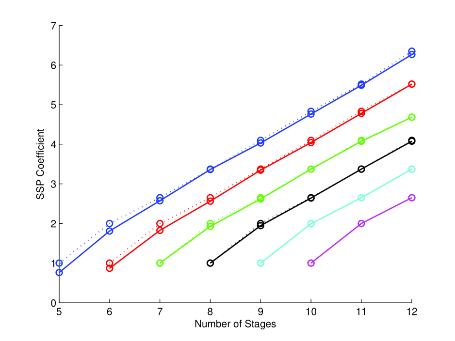
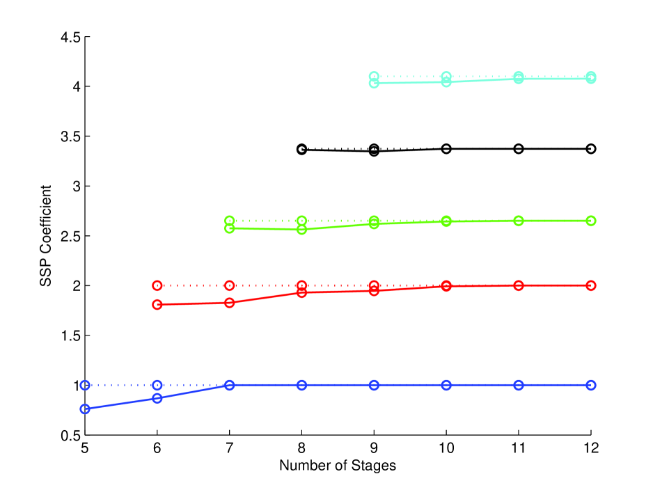
Table 2 shows the SSP coefficients of the $p=4$ methods for $5\leq p_{lin}\leq s\leq 12$. In bold are the coefficients that match those of the $p=2$ methods. In general, as we increase the number of stages the SSP coefficients for the $p=4$ methods approach those of the $p=2$ methods, as shown in Figure 2.

The tables clearly show that the size of the SSP coefficient depends on the relationship between $p_{lin}$ and $s$, so it is illuminating to look at the methods along the diagonals of these tables. Clearly, for $s=p_{lin}$ methods we have an optimal value of $\mathcal{C}=1$ and $\mathcal{C}_{\textup{eff}}=\frac{1}{s}$. The $p=2$ and $p=3$ methods all attain this optimal value, but for $p=4$ we have $\mathcal{C}_{(5,5,4)}=0.76$ and $\mathcal{C}_{(6,6,4)}=0.87$. However, once we get to a high enough number of stages, all the methods with $p=4$ and $s=p_{lin}=7,...,10$ that have $\mathcal{C}=1$ and $\mathcal{C}_{\textup{eff}}=\frac{1}{s}$. Figure 2 shows that for the linear methods ($p=2$) the SSP coefficient is fixed for $p_{lin}=s$ (blue dotted line), $p_{lin}=s-1$ (red dotted line), $p_{lin}=s-2$ (green dotted line), $p_{lin}=s-3$ (black dotted line), and $p_{lin}=s-4$ (cyan dotted line), and that the SSP coefficient of the corresponding $p=4$ methods (solid lines) approach these as the number of stages increases.

Figure 1: The SSP coefficient as a function of the number of coefficients for $p=2$ (dotted line) and $p=4$ (solid line) for $p_{lin}=5$ (blue), $p_{lin}=6$ (red), $p_{lin}=7$ (green), $p_{lin}=8$ (black), $p_{lin}=9$ (cyan), and $p_{lin}=10$ (magenta). As we increase the number of stages the SSP coefficients for the $p=4$ methods approach those of the $p=2$ methods

Figure 2: The SSP coefficient of linear methods $p=2$ (dotted line) and $p=4$ (solid line) for $p_{lin}=s$ (blue), $p_{lin}=s-1$ (red), $p_{lin}=s-2$ (green), $p_{lin}=s-3$ (black), and $p_{lin}=s-4$ (cyan). The SSP coefficient of the $p=4$ methods (solid lines) approach those of the corresponding $p=2$ method as the number of stages increases

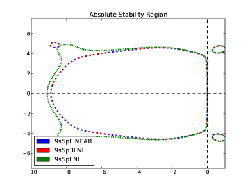
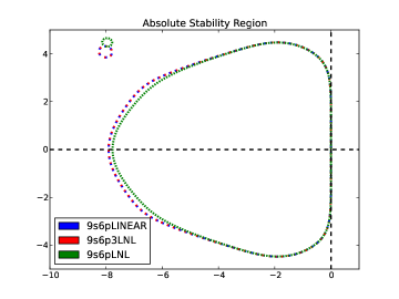
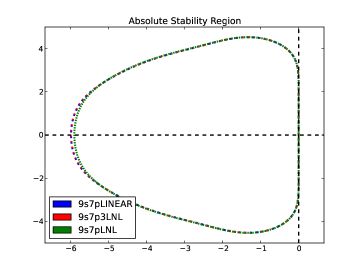
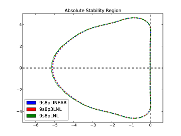
It is interesting to note that the linear stability regions of the $p=2$, $p=3$ methods are generally identical. The $p=4$ methods have stability regions that are virtually identical to those of the linear methods when the SSP coefficient is identical. In addition, methods with $s=p_{lin}$ and $p=4$ all have the same stability regions as the corresponding linear methods, which is not surprising as the stability polynomial of $s=p_{lin}$ is unique. For the rest of the methods, we observe that for a given number of stages $s$, as the linear order $p_{lin}$ increases the linear stability regions of the $p=4$ methods look closer to those of the linear methods. A nice illustration of this is the family of $s=9$ methods, shown in Figure 3.

It is known in the literature that some methods with nonlinear orders $p=3$ and $p=4$ achieve the linear threshold value. A nice example of this is Ketcheson’s SSP Runge–Kutta method of $s=10$, $p=p_{lin}=4$, which achieves the threshold value $\mathcal{C}=6.0$. This suggests that the linear order conditions are very significant to the value of the SSP coefficient. Indeed, we see this relationship in Tables 1 and 2, as we move right from column to column we see a significant drop in SSP coefficient. For each application, one must decide if a higher linear order is valuable, as we pay a price for requiring additional $p_{lin}$. However, once one has decided that the cost of a higher linear order is useful, there is no penalty in terms of SSP coefficient for requiring a higher nonlinear order $p=3$ and, in most cases, little reason not to use $p=4$. Our results show that if one wishes to use a method with high linear order $p_{lin}>4$, then requiring $p=3$ or even $p=4$ rather than the standard $p=2$ is not usually associated with significant restriction on the SSP coefficient. This can be beneficial in cases where the solution has linear and nonlinear components that need to be accurately captured simultaneously, or in different regions, or at different time-levels, so that the use of an SSP method that has optimal nonlinear order and higher linear order would be best suited for all components of the solution.

Figure 3: Linear stability regions of nine stage methods of linear orders $p_{lin}=5,6,7,8$ for linear (blue), $p=3$ (red) and $p=4$ (green) methods. The $p=4$ methods approach the $p=3$ and $p=2$ methods as $p_{lin}$ increases.

5 Numerical Results

In this section, the optimized LNL methods described in Section 4 are tested for convergence and SSP properties. First, we test these methods for convergence on both ODEs and PDEs to confirm that the new methods exhibit the desired linear and nonlinear orders. Next, we study the behavior of these methods in conjunction with a higher order WENO spatial discretizations, and show that although the WENO method is nonlinear, when applied to a linear smooth problem the higher order linear order $p_{lin}$ is beneficial. On the other hand, for nonlinear problems, both with shocks and without, the higher order nonlinear order $p=4$ is advantageous. Finally, the LNL methods are tested on linear and nonlinear problems with spatial discretizations that are provably total variation diminishing (TVD) and positivity preserving. We show that for the linear case, the observed time-step for the time stepping method to preserve the TVD property is well-predicted by the theoretical SSP coefficient, while for positivity and for the nonlinear problem the theoretical time-step serves as a lower bound.

Figure 4: Order verification of LNL Runge–Kutta methods on the van der Pol problem.

Figure 5: Order verification of LNL Runge–Kutta methods on a linear advection problem with Fourier spectral method in space.

Example 1: Nonlinear ODE convergence study. The van der Pol problem is a nonlinear system of ODEs:

$$u_{1}^{\prime}=u_{2}$$ (20)

$$u_{2}^{\prime}=\frac{1}{\epsilon}(-u_{1}+(1-u_{1}^{2})u_{2})$$ (21)

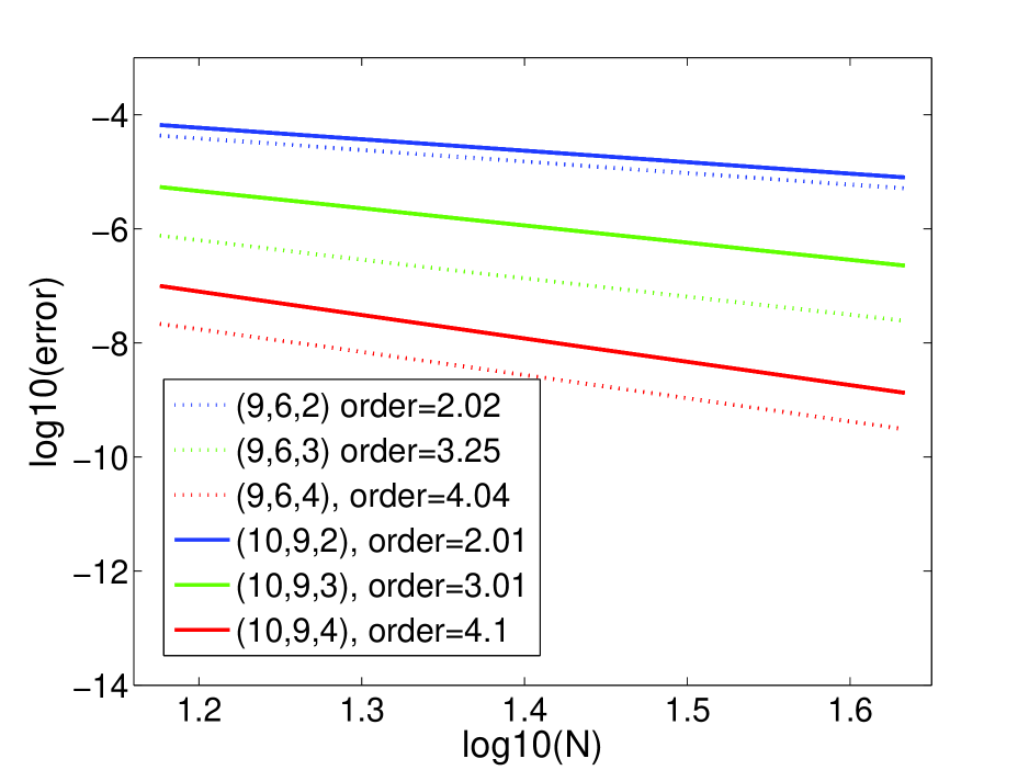
We use $\epsilon=10$ and initial conditions $u_{0}=(0.5;0)$. This was run using $(s,p_{lin},p)=$ (9,6,2), (9,6,3), (9,6,4), (10,9,2), (10,9,3), and (10,9,4) LNL Runge–Kutta methods to final time $T_{final}=4.0$, with $\Delta t=\frac{T_{final}}{N-1}$ where $N=15,19,23,27,31,35,39,43$. The exact solution (for error calculation) was calculated by MATLAB’s ODE45 routine with tolerances set to AbsTol=$10^{-14}$ and RelTol=$10^{-13}$. In Figure 5 we show that the $log_{10}$ of the errors in the first component vs. the $log_{10}$ of the number of points. The slopes of these lines (i.e the orders) are calculated by MATLAB’s polyfit function. As expected, the rate of convergence follows the nonlinear order of the method. In fact, we observe that a higher linear order is of no benefit at all for this example.

Example 2: PDE convergence study. In this study we solve the linear advection equation with sine wave initial conditions and periodic boundaries

$$u_{t} = -u_{x}\;\;\;x\in[0,1]$$ (22)

$$u(0,x) = \sin(4\pi x)\;\;\;\;u(t,0)=u(t,1)$$

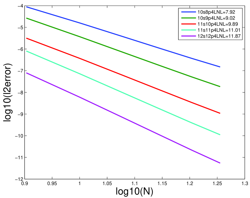
The Fourier spectral method was used to discretize in space using $N=(9,11,13,15,17,19)$ points. The exact solution to this problem is a sine wave with period $4$ that travels in time, so the Fourier spectral method gives us an exact solution in space [4] once we have two points per wavelength, allowing us to isolate the effect of the time discretization on the error. We run this problem for five methods with orders $p_{lin}=8,9,10,11,12$, $(s,p_{lin},p)=(10,8,4),(10,9,4),(11,10,4),(11,11,4),(12,12,4)$. Our final time is $T_{final}=1$, and the time step $\Delta t=0.9\Delta x$, where $\Delta x=\frac{1}{N-1}$. Errors are computed at the final time by comparison to the exact solution. Figure 5 shows the $log_{10}$ of the $l_{2}$ norm of the errors vs. $log_{10}$ of the number of points. The slopes of these lines (i.e the orders) are calculated by MATLAB’s polyfit function, and demonstrate that the methods achieved the expected linear convergence rates.

Figure 6: A linear advection problem with smooth solution and a WENO spatial discretization. On the left, $p=2$, on the right $p=4$. In both cases, the linear order dominates.

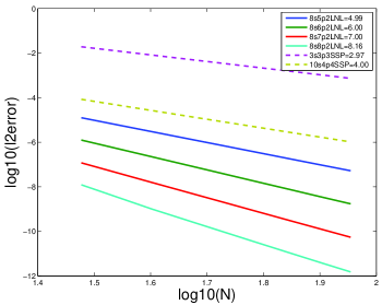
Example 3: Linear advection with WENO We repeat the example above, this time using the 15th order ($r=8$) WENO method to discretize in space with $\Delta x=\frac{1}{N-1}$ for $N=30,40,\dots,90$. The WENO method is a nonlinear method, so that even if the PDE is linear, the resulting system of ODEs is not. However, we can decompose the WENO method into a linear part and a nonlinear correction term that suppresses oscillations. In theory, when the equation is linear and solution is smooth, the WENO method is close to linear. We test this problem with selected LNL Runge–Kutta time discretizations of linear order $p_{lin}=5,6,7,8$ and $p=2,3,4$, and with the Shu-Osher SSP Runge–Kutta (3,3) and Ketcheson’s SSP Runge–Kutta (10,4). As above, our final time is $T_{final}=1$, and the time step $\Delta t=0.9\Delta x$, where $\Delta x=\frac{1}{N-1}$. Errors are computed at the final time by comparison to the exact solution. Figure 6 shows the $log_{10}$ of the $l_{2}$ norm of the errors vs. $log_{10}$ of the number of points, and the slopes of these lines (i.e the orders) as calculated by MATLAB’s polyfit function. We observe that the linear order dominates for this problem, which indicates that in regions where the problem is primarily linear and the solution smooth, the new LNL methods with higher linear orders could be of benefit.

Example 4: Burgers’ equation with WENO. In the previous example we demonstrated the advantages of using a time-stepping method with higher $p_{lin}$ with WENO in the case of a linear, smooth problem. In this example, we show how a higher nonlinear order $p$ is beneficial when dealing with a nonlinear equation with possibly discontinuous solution. Consider Burgers’ equation with symmetric sine wave initial conditions and periodic boundaries.

$$u_{t}+\left(\frac{1}{2}u^{2}\right)_{x}=0\;\;\;x\in[0,1]$$ (23)

$$u(0,x) = \sin(2\pi x)\;\;\;\;u(t,0)=u(t,1).$$

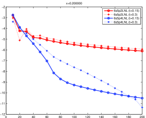
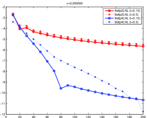
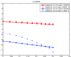
This problem develops a standing shock. We use a 15th order WENO scheme with $N$ points in space, and test the LNL time-stepping methods of linear order $p_{lin}=s-1=5,6,7$ and nonlinear order $p=2,3,4$. We use a time-step $\Delta t=0.45\Delta x$ where $\Delta x=\frac{1}{N-1}$.

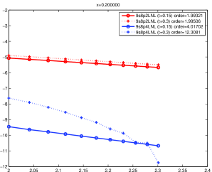
In Figure 7 we show the absolute values of the pointwise errors at spatial location $x=0.2$ for $N=10,\dots,200$ (top) and for $log_{10}(N)$ (bottom). These errors are shown before the shock forms (at time $T_{pre}=0.15$, solid line) and after the shock forms (at time $T_{post}=0.3$, dotted line). Observe that for smaller number of spatial points the errors decays very fast, however once we reach a spatial refinement that is small enough we see that the methods with higher $p$ have significantly smaller errors. If we consider only $N\geq 100$ points, we see the nonlinear order generally dominating: the linear methods feature second order convergence both pre- and post-shock, while the $p=4$ methods are fourth order pre-shock, but jump to twelfth order post-shock (probably capturing the high order WENO behavior). Taken together with the problem in Example 3, this suggests that using a method with high linear and high nonlinear order may be beneficial in examples that have smooth and linear regions and non-smooth nonlinear regions.

Figure 7: Burgers’ equation with WENO spatial discretization. Shown are pointwise errors at $x=0.2$, before (solid lines) and after (dotted line) the shock. The top figures show the $log_{10}$ of the errors vs. the number of points $N$. The bottom plots show the $log_{10}$ of the errors vs. $log_{10}(N)$ for $N\geq 100$. The time stepping methods use are $p_{lin}=s-1=5$ and $p_{lin}=s-1=8$ with nonlinear orders $p=2$ (red) and $p=4$ (blue). Clearly, methods with higher nonlinear order in time give smaller errors.

Example 5: Positivity and TVD time-step for a linear advection equation with first order finite difference in space. Consider the linear advection equation with a step function initial condition:

$$u_{t}+u_{x} =0\hskip 54.2025ptu(0,x)=\begin{cases}1,&\text{if }0\leq x\leq 1/2\\ 0,&\text{if }x>1/2\end{cases}$$

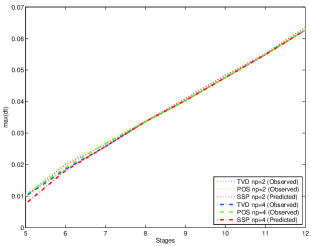
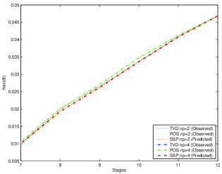
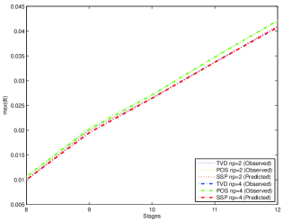
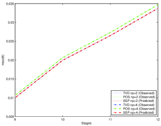
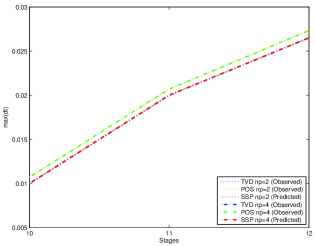
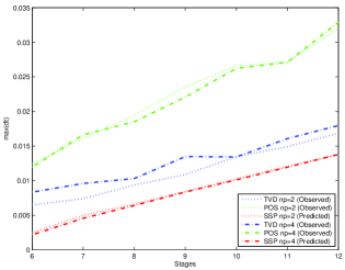
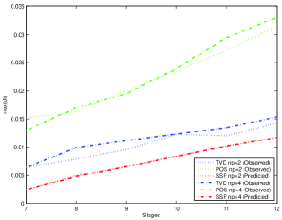
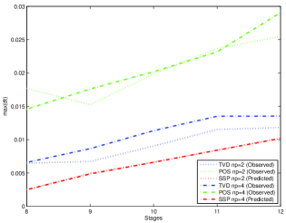
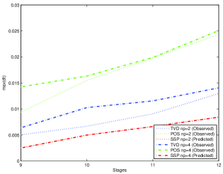
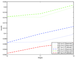
on the domain $[0,1]$ with periodic boundary conditions. We used a first-order forward difference to semi-discretized this problem on a grid with $N=101$ points and evolved it to a final time of $t=\frac{1}{8}$. For this problem it is known that Euler’s method is TVD and positive for step sizes up to $\Delta t_{\textup{FE}}=\Delta x$. We computed the numerical solution using all the $p=2$ and $p=4$ SSP LNL Runge–Kutta methods described in Section 4 and, for each one, found the largest $\Delta t$ for which TVD and positivity are preserved. In Figure 8 we plot these values (blue for TVD, green for positivity) compared to the time-step guaranteed by the theory, $\mathcal{C}\Delta t_{FE}$ (in red). We observe that the theoretical value is an excellent predictor of the observed TVD time-step; In fact, the blue line is frequently indistinguishable from the red line. The positivity preserving time-step is slightly larger, but follows a similar line.

Example 6: TVD and positivity for Buckley-Leverett with centered scheme and Koren limiter. We solve the Buckley-Leverett equation, a nonlinear PDE used to model two-phase flow through porous media:

$$u_{t}+f(u)_{x} =0, \text{ where }f(u)=\frac{u^{2}}{u^{2}+a(1-u)^{2}},$$

on $x\in[0,1]$, with periodic boundary conditions. We take $a=\frac{1}{3}$ and initial condition

$$u(x,0)=\begin{cases}1/2,&\text{if }x\geq 1/2\\ 0,&\text{otherwise.}\end{cases}$$ (24)

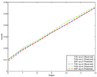
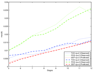
The problem is semi-discretized using a second order conservative scheme with a Koren Limiter as in [9] with $\Delta x=\frac{1}{100}$, and run to $t_{f}=\frac{1}{8}$. For this problem Euler’s method is TVD for $\Delta t\leq\Delta t_{FE}=\frac{1}{4}\Delta x=0.0025$. We computed the numerical solution using all the $p=2,3,4$ SSP LNL Runge–Kutta methods described in Section 4 and, as above found the largest $\Delta t$ for which TVD and positivity are preserved. In Figure 9 we plot these values (blue for TVD, green for positivity) compared to the time-step guaranteed by the theory, $\mathcal{C}\Delta t_{FE}$ (in red). The observed TVD and positivity time-step are typically significantly larger than the theoretical value. As before, the positivity preserving time-step is larger than the TVD time-step.

6 Conclusions

Using the optimization procedure described in [2, 5], we find SSP-optimized explicit Runge–Kutta methods that have nonlinear order of $p=3$ and $p=4$ and a higher $p_{lin}>4$ order of convergence on linear autonomous problems. The order barrier of $p\leq 4$ for explicit SSP Runge–Kutta methods indicates the critical importance of the nonlinear order on the SSP property. Nevertheless, we find that the size of the SSP coefficient is typically more constrained by the linear order conditions. As the number of stages increases, the SSP coefficient becomes primarily a function of the relationship between the number of stages and the linear order of the method, and not the nonlinear order. This means that in many cases, we can obtain methods of nonlinear order $p=4$ and linear order $p_{lin}>4$ that have the same SSP coefficient as methods with nonlinear order $p=2$ and linear order $p_{lin}>4$. We verified the linear and nonlinear orders of convergence of the new methods on a variety of test cases. We also showed the behavior of these new LNL time-stepping methods coupled with the WENO method for both linear and nonlinear problems, which suggests that these LNL methods may be useful for problems that have regions that are dominated by linear, smooth solutions and other regions where the solution is discontinuous or dominated by nonlinear behavior. Finally, we studied the total variation diminishing and positivity preserving properties of these LNL methods on linear and nonlinear problems, and showed that for the linear problems, the theoretical SSP time-step is a very accurate predictor of the observed behavior, while serving only as a lower bound in the nonlinear case. We conclude that where methods with high linear order are desirable, it is usually advantageous to pick those methods that also have higher nonlinear order ($p>2$).

Acknowledgment. The authors wish to thank Prof. Bram van Leer for the motivation for studying this problem, and Prof. David Ketcheson for many helpful discussions. This publication is based on work supported by AFOSR grant FA-9550-12-1-0224 and KAUST grant FIC/2010/05.

(a) Fifth order methods

(b) Sixth order methods

(c) Seventh order methods

(d) Eighth order methods

(e) Ninth order methods

(f) Tenth order methods

Figure 8: The time-step required for TVD (blue) and positivity (green) compared to the theoretical (red) for SSP linear (dotted) and LNL (dashed) Runge–Kutta methods of order $p_{lin}=5,...,10$ for a linear advection equation (Example 5).The red and blue lines overlap.

(a) Fifth order methods

(b) Sixth order methods

(c) Seventh order methods

(d) Eighth order methods

(e) Ninth order methods

(f) Tenth order methods

Figure 9: The time-step required for TVD (blue) and positivity (green) compared to the theoretical (red) for SSP linear (dotted) and LNL (dashed) Runge–Kutta methods of order $p_{lin}=5,...,10$ for a nonlinear PDE (Example 6).

References

- [1] S. Gottlieb and L.-A. Gottlieb, Strong stability preserving properties of Runge-Kutta time discretization methods for linear constant coefficient operators, Journal of Scientific Computing, 18 (2003), pp. 83–109.
- [2] S. Gottlieb, D. I. Ketcheson, and C.-W. Shu, Strong Stability Preserving Runge–Kutta and Multistep Time Discretizations, World Scientific Press, 2011.
- [3] S. Gottlieb and C.-W. Shu, Total variation diminishing runge–kutta methods, Mathematics of Computation, 67 (1998), pp. 73–85.
- [4] J. Hesthaven, S. Gottlieb, and D. Gottlieb, Spectral methods for time dependent problems, Cambridge Monographs of Applied and Computational Mathematics, Cambridge University Press, 2007.
- [5] D. I. Ketcheson, Rk-opt numerical optimization codes. https://github.com/ketch/RK-opt.
- [6] D. I. Ketcheson, Highly efficient strong stability preserving Runge–Kutta methods with low-storage implementations, SIAM Journal on Scientific Computing, 30 (2008), pp. 2113–2136.
- [7] D. I. Ketcheson, Computation of optimal monotonicity preserving general linear methods, Mathematics of Computation, 78 (2009), pp. 1497–1513.
- [8] D. I. Ketcheson, Runge-Kutta methods with minimum storage implementations, Journal of Computational Physics, 229 (2010), pp. 1763–1773.
- [9] D. I. Ketcheson, S. Gottlieb, and C. B. Macdonald, Strong stability preserving two-step runge-kutta methods, SIAM Journal on Numerical Analysis, (2012), pp. 2618–2639.
- [10] D. I. Ketcheson, D. Higgs, and S. Gottlieb, Strong stability preserving site. www.sspsite.org.
- [11] D. I. Ketcheson, C. B. Macdonald, and S. Gottlieb, Optimal implicit strong stability preserving Runge–Kutta methods, Applied Numerical Mathematics, 52 (2009), p. 373.
- [12] J. F. B. M. Kraaijevanger, Absolute monotonicity of polynomials occurring in the numerical solution of initial value problems, Numerische Mathematik, 48 (1986), pp. 303–322.
- [13] , Contractivity of Runge–Kutta methods, BIT, 31 (1991), pp. 482–528.
- [14] S. J. Ruuth and R. J. Spiteri, Two barriers on strong-stability-preserving time discretization methods, Journal of Scientific Computation, 17 (2002), pp. 211–220.
- [15] C.-W. Shu, Total-variation diminishing time discretizations, SIAM J. Sci. Stat. Comp., 9 (1988), pp. 1073–1084.
- [16] C.-W. Shu and S. Osher, Efficient implementation of essentially non-oscillatory shock-capturing schemes, Journal of Computational Physics, 77 (1988), pp. 439–471.
- [17] M. Spijker, Stepsize conditions for general monotonicity in numerical initial value problems, SIAM Journal on Numerical Analysis, 45 (2008), pp. 1226–1245.
- [18] R. J. Spiteri and S. J. Ruuth, A new class of optimal high-order strong-stability-preserving time discretization methods, SIAM J. Numer. Anal., 40 (2002), pp. 469–491.