The Stagger-grid: A Grid of 3D Stellar Atmosphere Models

Abstract

Aims. We present a theoretical study of the effects and signatures of realistic velocity field and atmospheric inhomogeneities associated with convective motions at the surface of cool late-type stars on the emergent profiles of iron spectral lines for a large range in stellar parameters.

Methods. We compute 3D spectral line flux profiles under the assumption of local thermodynamic equilibrium (LTE) by employing state-of-the-art, time-dependent, 3D, radiative-hydrodynamical atmosphere models from the Stagger-grid. A set of 35 real unblended, optical ${Fe\textsc{i}}$ and ${Fe\textsc{ii}}$ lines of varying excitation potential are considered. Additionally, fictitious ${Fe\textsc{i}}$ and ${Fe\textsc{ii}}$ lines ($5000\,\mathring{A}$ and $0,2,4\,\mathrm{eV}$) are used to construct general curves of growth and enable comparison of line profiles with the same line strength to illustrate systematical trends stemming from the intrinsic structural differences among 3D model atmospheres with different stellar parameters. Theoretical line shifts and bisectors are derived to analyze the shapes, shifts, and asymmetries imprinted in the full 3D line profiles emerging self-consistently from the convective simulations with velocity fields and atmospheric inhomogeneities.

Results. We find systematic variations in line strength, shift, width, and bisectors, that can be related to the respective physical conditions at the height of the line formation in the stellar atmospheric environment, in particular the amplitude of the vertical velocity field.

Conclusions. Line shifts and asymmetries arise due to the presence of convective velocities and the granulation pattern that are ubiquitously found in observed stellar spectra of cool stars.

1 Introduction

In recent years, capabilities for very high-resolution and very high signal-to-noise spectroscopical observations have raised the level of accuracy in stellar abundance analyses substantially (e.g., Asplund et al. 2005; Meléndez et al. 2009). In addition truly large-scale, comprehensive high-resolution spectroscopic surveys are currently conducted, and further ones are planned. For the accurate interpretation of these sterling data, improved theoretical atmosphere models were also needed.

Cool stars are characterized by convective envelopes that extend to the optical surface. The concomitant velocity field manifests itself in the stellar photosphere with a typical granulation pattern that imprints wavelength shifts and asymmetries in the observed spectral line profiles (e.g., Dravins et al. 1981; Nordlund et al. 2009). The strength of a spectral line depends mainly on the number of absorbers (atomic level population), therefore, it is very sensitive to the temperature due to exponential and power dependence of excitation and ionization equilibria (in LTE: $\propto e^{-\chi/kT}$; see Gray 2005 for more details on the theory of line formation in stellar atmospheres). In addition, owing to the presence of convective velocities, additional non-thermal broadening takes place in form of Doppler shifts. The wings of spectral lines are formed in deeper layers close to the continuum forming depth, while the cores are formed above in higher layers, therefore, the line profile samples different heights with distinctive physical conditions, in terms of velocity amplitudes, correlation between temperature and density inhomogeneities, asymmetries between regions with up- and downflowing material. This lead to characteristic asymmetries in the emergent intensity and flux line profiles (e.g., Asplund et al. 2000a).

Classical theoretical atmosphere models make use of several simplifications in order to facilitate calculations with the computing power at hand in the past (e.g., Gustafsson et al. 2008; Cassisi et al. 2004). The treatment of convection is a partially challenging part in modeling stellar atmospheres, since a complete theory of convection is still absent. In one-dimensional (1D) modeling, simplified treatments of convective energy transport have been adopted, such as the mixing-length theory (MLT; see Böhm-Vitense 1958; Henyey et al. 1965) or the full spectrum of turbulence model (Canuto & Mazzitelli 1991) with a priori unknown free-parameters that has to be calibrated by observations. Furthermore, for the 1D line formation calculations the lack of knowledge on the convective velocity fields is partially compensated by introducing two fudge parameters micro- and macroturbulence to account for convective broadening of spectral lines (e.g., Gray 2005).

For the precise modeling of realistic line profiles, including predicting their asymmetries, one has to rely on realistic three-dimensional (3D) atmosphere models, in which the convective velocity field emerges from first principles, i.e. from the solution of the hydrodynamic equations coupled with non-grey radiative transfer (e.g., Nordlund 1982; Steffen et al. 1989; Stein & Nordlund 1998; Vögler & Schüssler 2003; Nordlund et al. 2009; Freytag et al. 2012). A major application for 3D radiative hydrodynamic (RHD) atmosphere models is the computation of synthetic full 3D line profiles or spectra as post-processing based on the former in order to derive accurate stellar parameters and abundances (Asplund et al. 2000a, b, 2009). The 3D RHD models demonstrated their predictive capabilities powerfully in comparison with observed line profiles for several different stars. Asplund et al. (2000a) found almost perfect agreement between observed solar iron line profiles and theoretical predictions without any trends in the derived abundances with line strength. Furthermore, comparisons of line shifts and asymmetries derived from high-resolution spectroscopical observations of different types of cool stars advocated additionally for the realistic nature of the theoretical 3D RHD models (e.g., Nordlund & Dravins 1990; Atroshchenko & Gadun 1994; Allende Prieto et al. 2002; Ramírez et al. 2008, 2009, 2010; Gray 2009).

With the present theoretical work we intend to tackle the following key question: how do line properties vary with stellar parameters? More specifically, we intend to analyze line shifts and asymmetries carefully for a selection of ${Fe\textsc{i}}$ and ${Fe\textsc{ii}}$ lines, in order to better understand the variation of spectral line features with stellar parameters. Iron lines are often considered most useful for this purpose, since it is an abundant element with a very rich spectrum of energy levels and transitions with a variety of strengths and accurate atomic data at hand.

In Sec. 2 we explain the methods for the computations of the 3D atmosphere models and line profiles. Subsequently, we discuss the properties of lines in terms of shape, strength, width, and depth (Sec. 3, 4 and 5), as well as the line asymmetries and shifts (Sec. 6 and 7). In Sec. 8, we consider the physical conditions prevailing at the height of line forming region and link them with the findings on the line profiles. Finally in Sec. 9, we summarize our results.

2 3D atmosphere models and 3D spectral lines

Figure 1: Normalized disk-center ($\mu=1$) intensity profile as a function of wavelength for a single ${Fe\textsc{i}}$ line ($\lambda=5705.5,\,\chi_{\mathrm{exc}}=4.3$) with intermediate strength synthesized using the solar simulation (filled circles). The bisector information is plotted in the inset on the right-hand side of the figure. The line is decomposed into its contribution from upflows (blue) and downflows (red line), and the sum of both (black solid line).

Figure 2: Normalized flux vs. wavelength for a ${Fe\textsc{i}}$ ($\lambda=5705.5,\,\chi_{\mathrm{exc}}=4.3$; top panel) and ${Fe\textsc{ii}}$ line ($\lambda=5414.1,\,\chi_{\mathrm{exc}}=3.221$; bottom panel) with solid lines for different stellar parameters with an enlarged view of the bisector (dashed lines). In each column, only one stellar parameter is varied, while the other two are fixed (indicated); left panel: effective temperature; middle panel: surface gravity; right panel: metallicity. Furthermore, the respective lines computed with the $\left\langle\mathrm{3D}\right\rangle$ models are also shown (dotted lines). Note the different the ordinates between the top and bottom rows.

We have computed the Stagger-grid, a large grid of 3D RHD atmosphere models, which has been introduced in Magic et al. (2013a, hereafter paper I). The stellar parameters of the Stagger-grid span in effective temperature $T_{\mathrm{eff}}=[4000,7000]\,\mathrm{K}$ in steps of $500\,\mathrm{K}$, surface gravity $\log g=\left[1.5,5.0\right]$ in steps of 0.5 dex, and metallicity $\left[\mathrm{Fe}/\mathrm{H}\right]=\left[-4.0,+0.5\right]$ in steps of $0.5$ and $1.0\,\mathrm{dex}$. We employ a realistic equation-of-state (EOS) taken from (Mihalas et al. 1988), and the continuum and line opacity taken primarily from the MARCS package (Gustafsson et al. 2008). In the "star-in-a-box" setup, the rather small simulation box represents the statistical properties of the stellar subsurface and atmosphere. The numerical resolution of the Eulerian mesh of the box is $n_{xyz}=240^{3}$ for all Stagger-grid models. The horizontal boundaries are periodic and the vertical ones are open. The radiative transfer equation is solved along long characteristics for 8 inclined rays plus the vertical crossing for each grid-point at the surface of the simulation domain. The effects of non-grey radiative transfer are accounted for in the computations via the the opacity binning method (Nordlund 1982; Skartlien 2000), i.e. by sorting wavelengths into a number of opacity bins and properly averaging the opacities in each bin before solving the radiative transfer equation. We compute approximately two turn-over times, resulting in 100 - 150 equidistant snapshots. Furthermore, we obtain the mean $\left\langle\mathrm{3D}\right\rangle$ stratifications from the latter, with the temporal and spatial averaging methods as described in Magic et al. (2013b, hereafter paper II). For more details on the 3D atmosphere models we refer to paper I and II.

For the calculations of the spectral absorption line profiles, we utilize our 3D radiative transfer code Scate (Hayek et al. 2011). We consider a subset of 20 equidistant snapshots from the complete 3D simulation sequence and solve the radiative transfer along four polar $\mu$-angles, four azimutal $\varphi$-angles and the vertical for $n_{\lambda}=101$ wavelength points by applying consistently the same EOS and opacities as are used in the 3D atmosphere computations. In order to ease the computational burden for the individual line formation calculations, we assume local thermodynamic equilibrium (LTE), i.e. $S_{\lambda}=B_{\lambda}$, and neglect scattering. Furthermore, we reduce the number of columns in each direction from $240$ to 60, we have sorted that this does not alter the line profile noticeably, since the subsample is still large enough. The resulting intensity profiles are spatially averaged for each snapshot. In order to compute disk-averaged flux profiles, we integrate the various intensity profiles at all inclined angles using a Gauss-Legendre quadrature scheme. Lastly, we average the intensity and flux profiles temporally. In this work, we prefer to discuss flux profiles over intensity profiles, since the former are that what we observe in real stellar spectra except for the Sun, whose surface can be spatially resolved.

For this investigation we employ ${Fe\textsc{i}}$ and ${Fe\textsc{ii}}$ lines, which are the same as considered by Asplund et al. (2009). These lines consist of carefully selected unblended lines. In Table 1 we list the complete line list with their respective line parameters. From the total of 35 lines, 26 are from neutral (${Fe\textsc{i}}$), while 9 lines are from singly ionized iron (${Fe\textsc{ii}}$). As one can gather from the line parameters, we cover the visible wavelength range with $\lambda=\left[4445.5,8293.5\right]\,\mathring{A}$, and we match the ranges in lower excitation potential energy with $\chi_{\mathrm{exc}}=\left[0.087,4.608\right]\,\mathrm{eV}$ and oscillator strength with $\log gf=\left[-5.412,-1.355\right]$. For the solar simulation, the line strengths range from $W_{\lambda}=\left[9.2,64.3\right]\,\mathrm{m\mathring{A}}$, i.e. we cover from weak to intermediate line strength, however the $W_{\lambda}$ varies with stellar parameters, and we get stronger lines with a global maximum of $165.5\,\mathrm{m\mathring{A}}$.

In addition, we compute fictitious ${Fe\textsc{i}}$ and ${Fe\textsc{ii}}$ lines for a single wavelength ($\lambda=5000\,\mathring{A}$) covering three different lower excitation potential energies ($\chi_{\mathrm{exc}}=0,2,4\,\mathrm{eV}$) in order to facilitate a comparison between 3D models with different stellar parameters based on the same line strengths. For the so-called "curve-of-growth" method we consider ten equidistant $\log gf$ values resulting in a range of line strengths from weak to intermediate ($W_{\lambda}=5-100\,\mathrm{m\mathring{A}}$ for all models). We then interpolate the computed line profiles to construct a series of line profiles regularly distributed in line strength, from $W_{\lambda}=10$ to $100\,\mathrm{m\mathring{A}}$ in steps of $10\,\mathrm{m\mathring{A}}$. Finally, the line asymmetries (shift, width, depth and bisector) are determined from the resulting interpolated line profiles. The line shift is derived after the line profile is spline-interpolated to a finer resolution around the line core, while the bisector is determined for 100 points with spline interpolation.

3 Line shape

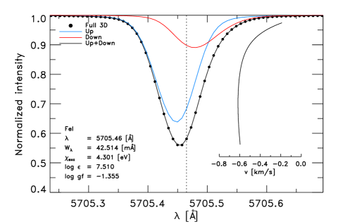
Real spectral absorption lines exhibit a more complex shape than just a Gaussian or Lorentzian profile due to the properties of the convective velocity field and inhomogeneities in the atmospheres of cool stars. In order to elucidate the individual contribution from the granules and the intergranular lane on the line shape and asymmetry, we show in Fig. 1 a ${Fe\textsc{i}}$ line computed from the solar simulation considering a single snapshot. We separated the line profiles of the individual columns into (bright) granules and (dark) intergranular lane (up- and downflows) based on a threshold at 90% from the mean continuum intensity. As expected, upflows show stronger blue-shifted profiles, while downflows have weaker, red-shifted lines (Asplund et al. 2000a). Furthermore, one can a notice distinct difference in the line depth of the individual components, which unveils the fact that the effect of the downflows is restricted mainly to the upper part of the bisector, while the lower part is predominantly contributed by the upflows in the granules.

In Fig. 2, we illustrate for a single ${Fe\textsc{i}}$ and ${Fe\textsc{ii}}$ line (top and bottom panel respectively) overviews of profiles including the bisectors, where one stellar parameter is varied, while the two others are fixed, in order to illustrate the individual influence of $T_{\mathrm{eff}},\,\log g$ and $\left[\mathrm{Fe}/\mathrm{H}\right]$ on the line shape and asymmetry.

The variations of line profiles and asymmetries with stellar parameters are systematic. Namely, the line strength decreases for ${Fe\textsc{i}}$ (increasing for ${Fe\textsc{ii}}$) with hotter $T_{\mathrm{eff}}$; the overall strength of spectral lines decreases, naturally, with lower $\left[\mathrm{Fe}/\mathrm{H}\right]$; asymmetries become more pronounced at higher $T_{\mathrm{eff}}$ and lower $\left[\mathrm{Fe}/\mathrm{H}\right]$ for both ${Fe\textsc{i}}$ and ${Fe\textsc{ii}}$. The opposing trends of the ${Fe\textsc{i}}$ and ${Fe\textsc{ii}}$ line strength with $T_{\mathrm{eff}}$ stems from the ionization of neutral iron at higher temperatures. In the case of the ${Fe\textsc{i}}$ line, line strength varies only marginally as $\log g$ decreases, while for ${Fe\textsc{ii}}$ line, the line strength increases significantly. In fact, the ${Fe\textsc{ii}}$ line strength shows always a clear rise for lower $\log g$, while for ${Fe\textsc{i}}$ lines this is the case only for cooler $T_{\mathrm{eff}}$, and hotter ones show even smaller trends with $\log g$. This behavior is easily understood if one considers that when most of the iron is in singly ionized form and ${Fe\textsc{i}}$ is a minority species, the line opacity is proportional to the electron number density which in turn is sensitive to the surface gravity. Also, in the atmospheres of late-type stars, the main source of continuum opacity in the optical is $\mathrm{H}^{-}$ and that also scales proportionally to the electron number density. Since the line strength of a normalized profile is proportional to the ratio of line and continuum opacity, this means that, to first-order approximation the dependence on electron density and, hence, on surface gravity cancels out in the case of ${Fe\textsc{i}}$ lines. Concerning the line shapes, towards giants (lower $\log g$) the asymmetries increase considerably for both lines due to the larger amplitude and velocity asymmetry between up- and downflows (see Fig. 8a). The wider and stronger line profiles in giants exhibit a more pronounced redshift in the upper bisector (see lines with $\log g=2.0$ in middle panel of Fig. 2) due to the increasing influence of the contribution from downflows on the red wing. For the highest $T_{\mathrm{eff}}$ ($6500\,\mathrm{K}$) or the lowest $\log g$ ($2.0$) the largest span in asymmetry is achieved for both lines (see Fig. 2; also bottom panel of Fig. 4b).

The height of line formation is in general very important, namely weaker lines show more pronounced line shifts and asymmetries, since they tend to form in deeper layers, where the maximum velocities and temperature contrasts happen ($\tau_{\mathrm{Ross}}\sim 1$; see Sec. 8). Stronger lines have their formation height shifted outwards where the velocity and contrast is lower and less well anti-correlated (see Fig. 8a). Similarly, ${Fe\textsc{ii}}$ lines are formed deeper than ${Fe\textsc{i}}$, since their number density increases in the deeper layers.

The wings are formed in deeper layers leading to a $/$-shape in the bisector arising from the granules (see Fig. 1), while the line core originates from higher layers. Therefore, with increasing line strength the line shift is receding after a maximum, leading to the $\backslash$-shape to the typical C-shape of the bisector (see Fig. 2). The line profile is often dominated by the granules, since these exhibit a brighter intensity, steeper temperature gradients and more importantly larger area contribution (filling factor) compared to the downflowing intergranular lane. However, this correlation decreases quickly above the optical surface, where convection ceases. Furthermore, the line shape and bisector depend on the vertical velocity field, its amplitude, asymmetry and the extent of overshooting into convective stable layers. The radial p-mode oscillations generally broaden the line profile, without however altering the overall line strength noticeably, since the nearly Lagrangian vertical oscillations do not influence the atmospheric stratification on an optical depth scale.

Additionally, we included in Fig. 2 also the symmetric line profiles resulting from the corresponding mean $\left\langle\mathrm{3D}\right\rangle$ models, in order to depict the influence from the inhomogeneities and in particular the vertical velocity field resulting from convection and granulation. The homogenous $\left\langle\mathrm{3D}\right\rangle$ models include micro- and macroturbulence in order to yield the same line strength and depth respectively as the considered full 3D line, therefore, one can isolate visually the Doppler shifts arising from the realistic 3D velocity field. At cooler $T_{\mathrm{eff}}$ the line shape is more symmetric, and the effects of velocities are rather small, while towards higher $T_{\mathrm{eff}}$ the differences grow more apparent. Due to the Doppler shifts the 3D lines are more blue-shifted.

4 Line strength

Figure 3: The relative difference between full 3D and $\left\langle\mathrm{3D}\right\rangle$ line strength, $\delta W_{\lambda}$, vs. $T_{\mathrm{eff}}$ averaged over all ${Fe\textsc{i}}$ and ${Fe\textsc{ii}}$ lines separately (top and bottom panel respectively).

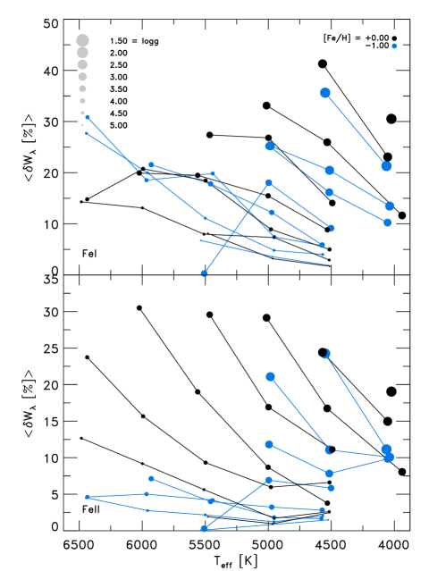
We evaluate the relative difference $\delta W_{\lambda}=W_{\mathrm{3D}}/W_{\left\langle\mathrm{3D}\right\rangle}-1$ between the predicted line strengths from the calculations with full 3D and with $\left\langle\mathrm{3D}\right\rangle$ models without any microturbulence. In Fig. 3, we display the average difference separated in ${Fe\textsc{i}}$ and ${Fe\textsc{ii}}$ lines with stellar parameters. We remark that the individual lines exhibit distinctive values between different lines, however, the average values depict qualitatively an overview of the variations. The difference $\delta W_{\lambda}$ quantifies the effects of atmospheric inhomogeneities as well as non-thermal Doppler broadening, since the $\left\langle\mathrm{3D}\right\rangle$ models include no velocity field or microturbulence. As expected the Doppler broadening due to the convective velocities is enhancing the line strength of the full 3D lines, with the consequence of the latter being stronger than the $\left\langle\mathrm{3D}\right\rangle$ lines. The enhancement in $W_{\lambda}$ is increasing for hotter $T_{\mathrm{eff}}$, lower $\log g$, and higher $\left[\mathrm{Fe}/\mathrm{H}\right]$, which corresponds to the variation of the vertical rms-velocity (see Fig. 8b). The trends of $\delta W_{\lambda}$ with stellar parameters are between ${Fe\textsc{i}}$ and ${Fe\textsc{ii}}$ in general qualitatively rather similar. Lines with higher excitation potential energy feature a smaller range in $\delta W_{\lambda}$.

5 Line width and depth

(a)

(b)

Figure 4: Left figure: Line width $l_{\mathrm{w}}$ (top) and depth $l_{\mathrm{d}}$ (bottom panel) derived from the flux profile of the fictitious ${Fe\textsc{i}}$ line ($W_{\lambda}=80\,\mathrm{m\mathring{A}},\,\chi_{\mathrm{exc}}=4.0\,\mathrm{eV}$) vs. effective temperature $T_{\mathrm{eff}}$ for different stellar parameters. Right figure: The mean (${Fe\textsc{i}}$) line shift and maximal bisector for different stellar parameters. Note the inverted ordinate in the top panel, which increases towards higher blue-shifts (negative velocity).

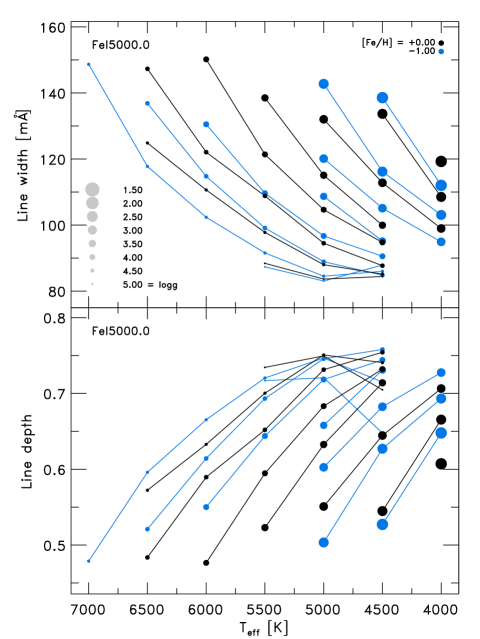
In order to study the intrinsic variations of shape of line profiles with stellar parameters, we determine the line width and depth from fictitious ${Fe\textsc{i}}$ lines with the same line strength ($W_{\lambda}=80\,\mathrm{m\mathring{A}}$). We define the line width, $l_{\mathrm{w}}$ as the full width at half maximum (FWHM) of the line profile, which is a measure of the range in Doppler shifts induced by the velocity field. From Fig. 4a (top panel), one can observe that the line width increases for higher $T_{\mathrm{eff}}$ and $\left[\mathrm{Fe}/\mathrm{H}\right]$, and lower $\log g$, which correlates with the variations of the vertical rms-velocity for the atmosphere models (see Fig. 8b). The line depth is the relative flux or intensity of the line core, $l_{\mathrm{d}}=1-\min\left[F_{\lambda}/F_{c}\right]$, and depicts the maximal absorption from the continuum radiation of a line. The line depth is clearly anti-correlated with the line width for different stellar parameters (bottom panel in Fig. 4a). However, the line depth declines faster than the line width rises, which signifies that the line profile is becoming flatter and broader, when considering the same line strength. This broadening of the line profile for different stellar parameters is a consequence of the higher velocity amplitudes (convection and oscillations) leading to larger Doppler shifts. The aspect ratio between depth and width, $a_{\mathrm{dw}}=l_{\mathrm{d}}/l_{\mathrm{w}}$, diminishes very quickly for hotter $T_{\mathrm{eff}}$, lower $\log g$ and $\left[\mathrm{Fe}/\mathrm{H}\right]$ for ${Fe\textsc{i}}$ lines. In the case of ${Fe\textsc{ii}}$ lines, the variation with $T_{\mathrm{eff}}$ is slightly different, namely the aspect ratio increases towards higher $T_{\mathrm{eff}}$ until $5500\,\mathrm{K}$ and drops above, and the largest $a_{\mathrm{dw}}$ being slightly smaller. In general the aspect ratio is increasing with $W_{\lambda}$, reaching a maximum around $50\,\mathrm{m\mathring{A}}$, and then decreasing, while for higher $\chi_{\mathrm{exc}}$ it is smaller. The changes of the width, depth and their aspect ratio are for $\left\langle\mathrm{3D}\right\rangle$ qualitatively similar, however their amplitude is rather different. This indicates that the flattening of line profile is partly due to thermal broadening as well.

6 Line asymmetry

Figure 5: Bisectors from fictitious ${Fe\textsc{i}}$ lines with three line strengths ($20,\,40$ and $80\,\mathrm{m\mathring{A}}$; top, middle and bottom panel, respectively) and three different excitation potential energies ($0,2,4\,\mathrm{eV}$; solid, dotted and dashed lines respectively) for different stellar parameters. In each column, one stellar parameter is varied, while the other two are fixed (indicated); left panel: effective temperature; middle panel: surface gravity; right panel: metallicity.

The bisector of a spectral line profile is the locus of the midpoints of the segments identified by the points at constant flux on the line profile. A line without asymmetries (e.g. 1D or $\left\langle\mathrm{3D}\right\rangle$ line) has a straight vertical bisector, while a realistic profile of a spectral line from a late-type stellar spectrum exhibits a bisector with the characteristic C-shape (Dravins et al. 1981) that results from the superposition of the contribution from the strong, blue-shifted, dominant granules and the weak, red-shifted, intergranular lanes (see Fig. 1).

In Fig. 3, we show ${Fe\textsc{i}}$ and ${Fe\textsc{ii}}$ bisectors for different stellar parameters. In general, the typical C-shape is present in most of the bisectors, however more or less pronounced depending on the line strength. Weak lines feature a blue-shifted bisector with a typical $/$-shape depicting only the upper part of the C-shape, where the line core coincides with the maximal line asymmetry, $\max\left[\left|v\right|\right]$, i.e. maximal absolute velocity shift of the entire bisector. On the other hand, the regions of formation of stronger lines cover larger ranges of optical depths and the cores of these lines are forming in higher layers above the overshooting region, therefore, the line centers are less blue-shifted and tend towards zero, thereby outlining a more defined C-shape. The maximal asymmetry of strong lines is located around the half height of the line depth.

For higher $T_{\mathrm{eff}}$ the bisectors increase significantly their range, while the line strength becomes weaker and also more blue-shifted, until the C-shape finally disappears ($6500\,K$). Towards giants (lower $\log g$) the line asymmetries (range of bisectors) become larger in general, and the C-shape is getting more pronounced until $\log g=3.0$ and less so below that. Furthermore, the upper part of the bisector recedes towards lower velocity shifts and are even red-shifted for the lowest surface gravity ($\log g=2.0$), since the contribution on the red wing from the downdraft is then dominating towards the continuum flux. With lower metallicity the lines are weaker and the bisectors lose their C-shape until it vanishes eventually. Also, the range in bisector diminishes. The variations in the line asymmetry with stellar parameters result from the differences in line strength, continuum level, filling factor and Doppler shift. We note that considering the variations of a single line with different stellar parameters changes significantly its shape (see Fig. 2).

In Fig. 5 we illustrate bisectors from the fictitious ${Fe\textsc{i}}$ line flux profiles for different stellar parameters, with the same line strength, considering weak ($20,\,40\,\mathrm{m\mathring{A}}$) and intermediate ($80\,\mathrm{m\mathring{A}}$) line strength (top, middle and bottom panel, respectively). The basic idea behind this comparison is to isolate and illustrate the effect and signature on the line profile due to the intrinsic structural differences among individual 3D atmosphere models arising solely from the variations in the convective flow properties. We vary one stellar parameter individually, while the other two are fixed ($T_{\mathrm{eff}}$, $\log g$ and $\left[\mathrm{Fe}/\mathrm{H}\right]$). Three different excitation potential energies ($\chi_{\mathrm{exc}}=0,2,4$ eV) are also considered (solid, dotted and dashed, respectively).

The intermediate strong lines feature often a more explicit C-shape compared to the weak lines with smaller maximal bisectors, otherwise, the changes with stellar parameters are qualitatively rather similar. For hotter $T_{\mathrm{eff}}$ and lower $\log g$, their effect on the weak and intermediate strong lines is rather similar, namely the line depth is decreasing (for the same line strength) and the line width is rising, which means that the line shape becomes increasingly flatter and broader (see also Sec. 5), while the line shift and maximal bisector is considerably enhanced, primarily due to concomitant higher velocity and $T$-contrast (see Sec. 8). On the other hand, at lower metallicity the changes in line shape are less pronounced, only the exhibited blue-shifts are lower due to the smaller level in velocity and $T$-contrast. In the case of the weak lines (top panel) with lower $T_{\mathrm{eff}}$ and $\left[\mathrm{Fe}/\mathrm{H}\right]$, higher $\log g$ the bisectors are increasingly uniform over the entire line depth, and the C-shape is less distinct, since weak lines are arising from a smaller extent in height. The variations of the fictitious ${Fe\textsc{ii}}$ are rather similar to those by ${Fe\textsc{i}}$, therefore we refrain from showing them. The only noteworthy differences are the slightly smaller ranges in line shift, depth and maximal bisector for fictitious ${Fe\textsc{ii}}$ lines, and the fact that giants feature a stronger influence from the red-shifted downflows. Lines with higher excitation potential energy show in general more blue-shifted bisectors, since these lines form in deeper layers with higher velocity and temperature contrasts.

Figure 6: The maximal bisector vs. maximal vertical rms-velocity for different stellar parameters. A linear fit is included (red line).

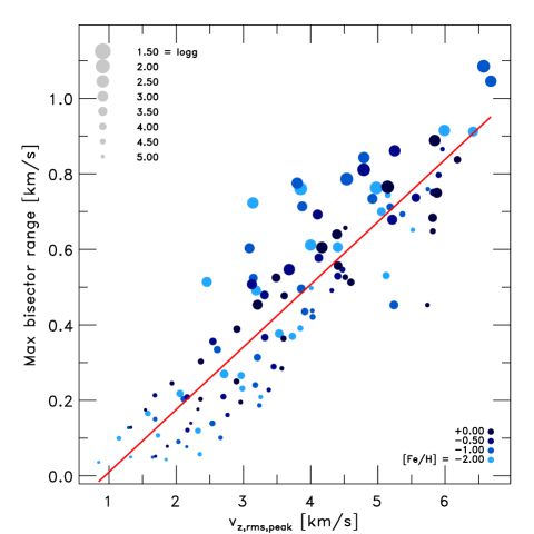
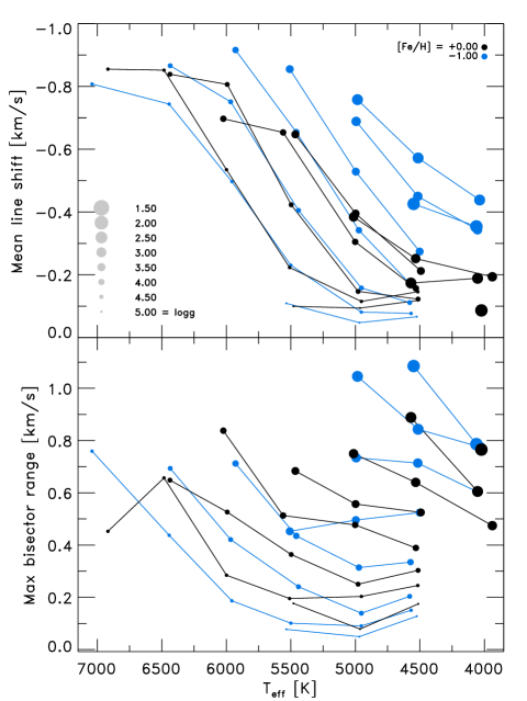
In Fig. 4b (bottom panel) we show the maximal range of the bisectors with stellar parameters, which are increasing for higher $T_{\mathrm{eff}}$ and $\left[\mathrm{Fe}/\mathrm{H}\right]$, lower $\log g$ similar to the vertical rms-velocity in the 3D atmosphere models (see Fig. 8a). One would assume the line asymmetries correlate with the velocity field, since these arise from the Doppler shifts. Therefore, we compare the maximal range of the bisectors with the maximal vertical rms-velocity for different stellar parameters in Fig. 6. The line asymmetries correlate clearly with amplitude of the vertical velocity, only there is a slight scatter due to the different heights of line formation.

7 Line shift

Figure 7: Line core shift vs. line strength for the ${Fe\textsc{i}}$ and ${Fe\textsc{ii}}$ lines (circles and triangles, respectively) for different stellar parameter. Also, the corresponding trends for fictitious ${Fe\textsc{i}}$ and ${Fe\textsc{ii}}$ lines are shown (blue solid and dashed lines). The excitation potential energy $\chi_{\mathrm{exc}}$ (blue colors, where lighter refers to higher $\chi_{\mathrm{exc}}$) and wavelength $\lambda$ are indicated (symbol sizes, where bigger refers to higher $\lambda$). In each row, one stellar parameter is varied, while the other two are fixed (indicated); top panel: effective temperature; middle panel: surface gravity; bottom panel: metallicity.

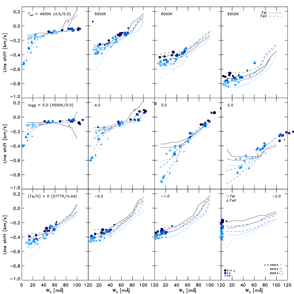
In Fig. 4b (top panel), we show an overview of the mean line shift of the ${Fe\textsc{i}}$ lines with stellar parameters. Furthermore, we show in Fig. 7 an overview of the line shift against the line strength for various stellar parameters, in order to depict the influence of $T_{\mathrm{eff}}$, $\log g$ and $\left[\mathrm{Fe}/\mathrm{H}\right]$ individually (from top to bottom respectively) for the complete ${Fe\textsc{i}}$ and ${Fe\textsc{ii}}$ line set (circles and triangles respectively). The lower excitation potential energy, $\chi_{\mathrm{exc}}$, and line wavelength of the lines are indicated to illustrate trends with line parameters (blue colors and symbol size respectively).

In the following we discuss the ${Fe\textsc{i}}$ lines first. Towards hotter effective temperatures (top panel of Fig. 7) we find the maximum shifts of ${Fe\textsc{i}}$ lines to rise considerably (from $\sim 0.1$ to $0.8\,\mathrm{km/s}$), while the maximal line strength is diminishing (from $140$ to $40\,\mathrm{m\mathring{A}}$). At higher $T_{\mathrm{eff}}$, one finds convection to operate less efficiently and therefore with more vigorous flows, with both higher $T$-contrast and rms-velocity (Fig. 8a). On the other hand, at higher $T_{\mathrm{eff}}$, iron is more likely to be ionized and also the (continuum) $\mathrm{H}^{-}$-opacity increases, hence, both effects are reducing the line strength. We note that weaker lines typically originate from lower depth, where the velocity and $T$-contrast are larger, therefore imprinting a larger line shift. The line cores of stronger lines form higher up in the atmosphere, therefore, their line shifts are smaller (notice the generally smaller line shifts towards stronger lines in Fig. 7). Moreover, for higher $T_{\mathrm{eff}}$ the range in line shift is decreasing. For lower surface gravity (middle panel), the line shift, its range and the slope of the linear fits are increasing, reach a maximum at $\log g=3.0$ and decrease again, while the range in line strength is almost unaffected. For lower metallicity (bottom panel), the line shifts and line strength are reducing, and the slope of the linear fit are becoming steeper.

We find in general that the line shifts and strengths are anti-correlated, i.e. for weaker (stronger) lines their shifts are higher (lower), which arises from the deeper (higher) location of line formation, and the respectively larger (lower) velocity amplitude. On the other hand, lines with lower (higher) excitation potential energy, $\chi_{\mathrm{exc}}$, exhibit smaller (larger) line shifts. The lines are on average blue-shifted (negative line shift; see top panel of Fig. 4b), since the granules occupy a higher filling factors and intensity contribution over downdrafts. The mean line shift is increasing for higher $T_{\mathrm{eff}}$, lower $\log g$ and enhanced $\left[\mathrm{Fe}/\mathrm{H}\right]$. Only a few of the strongest lines in giants exhibit red-shifted line cores, since the relative contribution of the red-shifted downflows in these are pronounced. We find that the fictitious ${Fe\textsc{i}}$ and ${Fe\textsc{ii}}$ lines have qualitatively very similar line shifts as the mean line shifts shown in Fig. 4b. The latter show a distinct dependence on the line strength.

The ${Fe\textsc{ii}}$ lines exhibit in general similar trends for line strength and shift with stellar parameter as found for the ${Fe\textsc{i}}$ lines. However, the ranges in line strength are distinctively smaller and its variations are much less pronounced, in particular the line strength is less sensitive to $T_{\mathrm{eff}}$, since it is the majority species. Furthermore, the mean line shift and the slope of the linear fits are in general higher compared to the ${Fe\textsc{i}}$ values.

8 Conditions at the height of line formation

(a)

(b)

Figure 8: Left figure: The vertical rms-velocity and its asymmetry (top); $T$-constrast and its asymmetry (middle); correlation function $C\left[v_{z},T\right]$ and filling factor (bottom panel) shown against the optical depth for models with $\log g=4.5$ and solar metallicity. The different $T_{\mathrm{eff}}$’s are color-coded (red/orange colors). Right figure: Maximal vertical rms-velocity and maximal temperature contrast vs. $T_{\mathrm{eff}}$ (top and bottom panel respectively) for different stellar parameters.

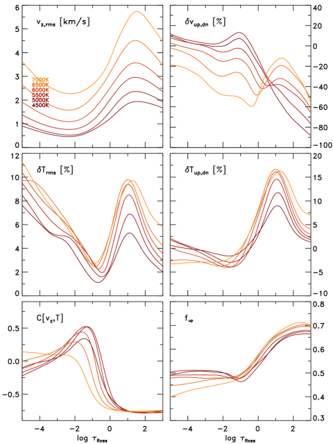
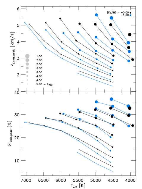
In the following we want to discuss the different physical conditions based on the properties of the velocity and temperature prevailing in the 3D RHD model atmospheres, which are in the end responsible for the various line asymmetries we seen above. In Fig. 8a, we show the vertical rms-velocity, $v_{z,\mathrm{rms}}$, the asymmetry between up- and downflow rms-velocity, $\delta v_{\mathrm{up,dn}}$, temperature contrast, $\delta T_{\mathrm{rms}}$, the temperature difference between up- and downflows, $\delta T_{\mathrm{up,dn}}$, the correlation function of the temperature and vertical velocity, $C\left[v_{z},T\right]$, and the filling factor of the upflows $f_{\mathrm{up}}$.

In the superadiabatic region (SAR) just below the optical surface ($\log\tau_{\mathrm{Ross}}>0$) the vertical rms-velocities and temperature contrasts are reaching their maxima, since at the thin photospheric transition region the radiative losses from the upflows generate large entropy fluctuations, that drive stellar surface convection (see paper I and Nordlund et al. 2009, for more details). Further above the top of the convection zone, $v_{z,\mathrm{rms}}$ and $\delta T_{\mathrm{rms}}$ decline with height. Also, the asymmetries between the up- and downflows in velocity and temperature drop fast with height, while in convection zone, in particular the SAR, $\delta v_{\mathrm{up,dn}}$ and $\delta T_{\mathrm{up,dn}}$ are rather large. Furthermore, below the optical surface, one finds a tight anti-correlation between the vertical rms-velocity and temperature due to convective transport of energy, while above the correlation is distinctively smaller (see $C\left[v_{z},T\right]$ in Fig. 8a). The extent of overshooting can be determined with the zero crossing of the correlation function, $C\left[v_{z},T\right]$, and for higher $T_{\mathrm{eff}}$’s with concomitant higher velocity the overshooting is clearly shifting towards higher layers. On the other hand, the convective properties obviously change with stellar parameters. In order to illustrate this, we show the maxima of $v_{z,\mathrm{rms}}$ and $\delta T_{\mathrm{rms}}$ in Fig. 8b for different stellar parameters. Both quantities clearly increase for hotter $T_{\mathrm{eff}}$, lower $\log g$, and higher metallicity (see Paper I for a detailed discussion).

Therefore, one finds in general that lines forming in deeper layers carry larger signatures from the velocity field and temperature contrast, i.e. resulting in larger line broadening and Doppler shifts, and in higher layers the opposite is the case. And also the variations of the line shifts and asymmetries with stellar parameters, which we discussed above, are in agreement with the properties in the 3D RHD models.

9 Conclusions and summary

We have explored the properties of synthetic spectral lines from neutral and singly ionized iron in late-type stars with the aid of 3D hydrodynamical model atmospheres. We have studied the variations with stellar parameters of aspects such as the strength, width, and depth of spectral lines, as well as line asymmetries and wavelength shifts. We have related such variations and the morphology of the asymmetries to the structural and thermal properties of the 3D models, with particular focus on velocity and temperature inhomogeneities and their correlation with depth in the stellar atmosphere.

In Table 2 we list our results (line strength, shift, width, depth and bisectors). A possible application of the theoretical predictions of the line asymmetries can be the derivation of radial velocity and gravitational red-shift from high resolution observations by comparison with 3D line bisectors.

Appendix A Tables

Table 1: The he ${Fe\textsc{i}}$ and ${Fe\textsc{ii}}$ line parameters with reference number, ionization degree, wavelength $\lambda$, lower excitation potential $\chi_{\mathrm{exc}}$, oscillator strength $\log gf$, weighting factor $g_{u}$, radiation damping $\log\gamma_{\mathrm{rad}}$, lower level $l_{l}$, upper level $l_{u}$.

#	id	$\lambda$	$\chi_{\mathrm{exc}}$	$\log gf$	$g_{u}$	$\log\gamma_{\mathrm{rad}}$	$l_{l}$	$l_{u}$
1	1	4445.4717	0.087	-5.412	1	4.22	s	p
2	1	5247.0503	0.087	-4.961	1	3.63	s	p
3	1	5491.8315	4.186	-2.188	2	8.09	d	p
4	1	5600.2242	4.260	-1.420	2	8.01	p	s
5	1	5661.3457	4.284	-1.756	2	8.00	p	s
6	1	5696.0896	4.548	-1.720	2	8.33	p	d
7	1	5705.4648	4.301	-1.355	2	8.38	p	s
8	1	5778.4531	2.588	-3.440	2	8.21	s	p
9	1	5784.6582	3.396	-2.532	3	8.05	p	s
10	1	5855.0767	4.608	-1.478	2	8.33	p	d
11	1	5956.6943	0.859	-4.552	1	4.00	s	p
12	1	6151.6182	2.176	-3.282	1	8.29	s	p
13	1	6240.6460	2.223	-3.287	3	6.81	s	p
14	1	6311.5003	2.831	-3.141	2	8.20	s	p
15	1	6498.9390	0.958	-4.695	1	4.36	s	p
16	1	6518.3671	2.831	-2.448	2	8.21	s	p
17	1	6574.2285	0.990	-5.010	1	4.22	s	p
18	1	6609.1104	2.559	-2.682	1	7.99	s	p
19	1	6699.1416	4.593	-2.101	2	8.09	s	p
20	1	6739.5220	1.557	-4.794	3	7.24	s	p
21	1	6793.2593	4.076	-2.326	2	7.56	d	p
22	1	6837.0059	4.593	-1.687	2	7.85	s	p
23	1	6854.8228	4.593	-1.926	2	7.81	s	p
24	1	7401.6851	4.186	-1.500	2	8.01	d	p
25	1	7912.8670	0.859	-4.848	1	3.68	s	p
26	1	8293.5146	3.301	-2.203	2	8.20	s	p
27	2	4620.5129	2.828	-3.210	31	8.56	s	p
28	2	5264.8042	3.230	-3.130	31	8.56	s	p
29	2	5414.0717	3.221	-3.580	31	8.56	s	p
30	2	6432.6757	2.891	-3.570	31	8.49	s	p
31	2	6516.0767	2.891	-3.310	31	8.49	s	p
32	2	7222.3923	3.889	-3.260	31	8.56	s	p
33	2	7224.4790	3.889	-3.200	31	8.56	s	p
34	2	7515.8309	3.903	-3.390	31	8.56	s	p
35	2	7711.7205	3.903	-2.500	31	8.56	s	p

In Table 1, we present the ${Fe\textsc{i}}$ and ${Fe\textsc{ii}}$ line parameters that are used for the line formation calculations, in the present work. While in Table 2 we show a subset from the main results we presented in our work retrieved for the solar simulation. The complete list is online available on CDS.

Table 2: Table with main results from synthetic spectral flux profiles: line strength, width, depth, shift, minimum and maximum of bisector for the solar simulation. The line number in the first column is the same as used in Table 1.

#	$W_{\lambda}$	$l_{\mathrm{s}}$	$l_{\mathrm{w}}$	$l_{\mathrm{d}}$	min	max
1	43.948	-0.374	4.850	0.561	-0.373	-0.248
2	67.517	-0.192	5.381	0.664	-0.276	-0.195
3	13.965	-0.501	4.867	0.145	-0.500	-0.288
4	41.099	-0.420	5.213	0.382	-0.432	-0.241
5	25.989	-0.475	5.040	0.246	-0.473	-0.247
6	18.203	-0.476	5.037	0.172	-0.490	-0.254
7	43.520	-0.420	5.312	0.385	-0.421	-0.242
8	24.787	-0.432	4.757	0.248	-0.431	-0.254
9	30.014	-0.440	4.965	0.282	-0.434	-0.237
10	25.239	-0.483	5.108	0.227	-0.473	-0.249
11	54.501	-0.272	4.997	0.505	-0.303	-0.202
12	51.801	-0.310	5.085	0.453	-0.332	-0.203
13	49.442	-0.315	5.027	0.432	-0.337	-0.204
14	28.465	-0.422	4.802	0.258	-0.412	-0.235
15	45.180	-0.318	4.802	0.399	-0.321	-0.214
16	59.973	-0.286	5.283	0.476	-0.308	-0.191
17	29.505	-0.375	4.595	0.267	-0.371	-0.224
18	63.179	-0.224	5.325	0.487	-0.295	-0.190
19	8.560	-0.481	4.802	0.073	-0.481	-0.237
20	16.198	-0.392	4.541	0.145	-0.403	-0.236
21	14.832	-0.442	4.880	0.122	-0.443	-0.243
22	18.876	-0.473	4.880	0.155	-0.463	-0.226
23	12.255	-0.476	4.807	0.102	-0.474	-0.229
24	44.531	-0.357	5.134	0.317	-0.360	-0.203
25	48.607	-0.280	4.773	0.353	-0.291	-0.187
26	58.154	-0.297	5.216	0.360	-0.306	-0.193
27	56.562	-0.352	5.702	0.584	-0.425	-0.279
28	45.612	-0.372	5.453	0.433	-0.414	-0.259
29	28.478	-0.495	5.210	0.278	-0.487	-0.264
30	42.298	-0.314	5.268	0.341	-0.344	-0.209
31	53.208	-0.247	5.458	0.410	-0.306	-0.205
32	19.331	-0.456	5.141	0.143	-0.470	-0.226
33	21.188	-0.448	5.141	0.156	-0.457	-0.226
34	15.578	-0.488	5.105	0.112	-0.483	-0.224
35	48.518	-0.238	5.437	0.312	-0.304	-0.204