On Compressive Sensing in Coding Problems: A Rigorous Approach

Wasim Huleihel,  Neri Merhav,  Shlomo Shamai (Shitz)
Department of Electrical Engineering
Technion - Israel Institute of Technology
Haifa 32000, ISRAEL
E-mail: {wh@tx, merhav@ee, sshlomo@ee}.technion.ac.il
The work of Huleihel and Merhav was partially supported by The Israeli Science Foundation (ISF), Grant no. 412/12. The work of Shamai was supported by The Israeli Science Foundation (ISF), the European Commission in the framework of the FP7 Network of Excellence in Wireless COMmunications NEWCOM# and by S. and N. Grand Research Fund.
Abstract

We take an information theoretic perspective on a classical sparse-sampling noisy linear model and present an analytical expression for the mutual information, which plays central role in a variety of communications/processing problems. Such an expression was addressed previously either by bounds, by simulations and by the (non-rigorous) replica method. The expression of the mutual information is based on techniques used in [1], addressing the minimum mean square error (MMSE) analysis. Using these expressions, we study specifically a variety of sparse linear communications models which include coding in different settings, accounting also for multiple access channels and different wiretap problems. For those, we provide single-letter expressions and derive achievable rates, capturing the communications/processing features of these timely models.

Index Terms:
Channel coding, state dependent channels channel, wiretap channel, multiple access channel (MAC), replica method, random matrix theory.

I Introduction

Compressed sensing [2, 3] is a collection of signal processing techniques that compress sparse analog vectors by means of linear transformations. Using some prior knowledge on the signal sparsity, and by designing efficient encoders and decoders, the goal is to achieve effective compression in the sense of taking a much smaller number of measurements than the dimension of the original signal. Recently, a vast amount of research was conducted concerning sparse random Gaussian signals which are very relevant to wireless communications, see, for example, [1, 4, 5, 6] and many references therein.

A general setup of compressed sensing is shown in Fig. 1. The mechanism is as follows: A real vector 𝑿n𝑿superscript𝑛\mbox{\boldmath$X$}\in\mathbb{R}^{n} is mapped into 𝑽k𝑽superscript𝑘\mbox{\boldmath$V$}\in\mathbb{R}^{k} by an encoder (or compressor) f:nk:𝑓superscript𝑛superscript𝑘f:\mathbb{R}^{n}\to\mathbb{R}^{k}. The decoder (decompressor) g:kn:𝑔superscript𝑘superscript𝑛g:\mathbb{R}^{k}\to\mathbb{R}^{n} receives 𝒀𝒀Y, which is a noisy version of 𝑽𝑽V, and outputs 𝑿^^𝑿\hat{\mbox{\boldmath$X$}} as the estimation of 𝑿𝑿X. The sampling rate, or the compression ratio, is defined as

q=kn.superscript𝑞𝑘𝑛\displaystyle q\stackrel{{\scriptstyle\triangle}}{{=}}\frac{k}{n}. (1)

In this paper, the encoder is constrained to be a linear mapping, denoted by a matrix 𝑯k×n𝑯superscript𝑘𝑛\mbox{\boldmath$H$}\in\mathbb{R}^{k\times n}, usually called the sensing matrix or measurement matrix, where 𝑯𝑯H is assumed to be a random matrix with i.i.d. entries of zero mean and variance 1/n1𝑛1/n. On the decoder side, most of the compressed sensing literature focuses on low-complexity decoding algorithms which are robust to noise, for example, decoders based on convex optimization, greedy algorithms, etc. (see, for example [5, 7, 8, 9]). Although the decoding is, of course, an important issue, it is not in the focus of this work. The input vector 𝑿𝑿X is assumed to be random, distributed according some probability density that models the sparsity. Finally, the noise is assumed to additive white and Gaussian.

Encoderfn:nk:subscript𝑓𝑛superscript𝑛superscript𝑘f_{n}:\;\mathbb{R}^{n}\to\mathbb{R}^{k}Decodergn:kn:subscript𝑔𝑛superscript𝑘superscript𝑛g_{n}:\;\mathbb{R}^{k}\to\mathbb{R}^{n}𝑿^^𝑿\hat{\mbox{\boldmath$X$}}𝒀𝒀Y𝑾𝑾W𝑽𝑽V𝑿𝑿X
Figure 1: Noisy compressed sensing setup.

In the literature, there is a great interest in finding asymptotic formulas of some information and estimation measures, e.g., the minimum mean squared error (MMSE), mutual information rates, and other information measures. Finding these formulas is, in general, extremely complicated, and most of the works (e.g., [4, 6, 10]) that deal with this problem resort to using the replica method which is borrowed from the field of statistical physics. Although the replica method is powerful, it is non-rigorous. Recently, in [1] a rigorous derivation of the asymptotic MMSE was carried out, and it was shown that the results obtained support the previously known replica predictions. The key idea in our analysis is the fact that by using some direct relationship between optimum estimation and certain partition functions [11], the MMSE can be represented in some mathematically convenient form which (due to the previously mentioned input and noise Gaussian statistics assumptions) consists of functionals of the Stieltjes and Shannon transforms. This observation allows us to use some powerful results from random matrix theory, concerning the asymptotic behavior (a.k.a. deterministic equivalents) of the Stieltjes and Shannon transforms (see e.g., [12, 13] and many references therein). Here, however, we are concerned with some input-output mutual information rates, rather than the asymptotic MMSE. Nonetheless, we show that these information rates are readily obtained from the results of [1]. It is worthwhile to emphasize that these kind of mutual information rates formulas are useful and important. For example, with relation to this paper, recently, in [14], the capacity was derived for single-user discrete-time channels subject to both frequency-selective and time-selective fading, where the channel output is observed in additive Gaussian noise. This result is indeed important due to the fact that various mobile wireless systems are subject to both frequency-selective fading and to time-selective fading.

The works cited above focus on uncoded continuous signals, while in this paper, we concentrate on coded communication, similarly to [15]. In other words, we use coded sparse signals, and the objective is to achieve reliable reconstruction of the signal and its support. In [15], sparse sampling of coded signals at sub-Landau sampling rates was considered. It was shown that with coded and with discrete signals, the Landau condition may be relaxed, and the sampling rates required for signal reconstruction and for support detection can be lower than the effective bandwidth. Equivalently, the number of measurements in the corresponding sparse sensing problem can be smaller than the support size. Tight bounds on information rates and on signal and support detection performance are derived for the Gaussian sparsely sampled channel and for the frequency-sparse channel using the context of state dependent channels. It should be emphasized that part of the coding principles and problems that we will consider in this paper have already appeared in [15], but relying on bounds. Here, the new results facilitate a rigorous discussion.

The main goal of this paper is to use the previously mentioned mutual information rates in order to give some new closed-form achievable rates in various channel coding problems, in the wiretap channel model, and in the multiple access channel (MAC). Particularity, in the first part of these channel coding problems, we will consider three different cases that differ in the assumptions about the knowledge available at the transmitter and the receivers. For example, in Subsection IV-B, we will consider the case in which the sparsity pattern cannot be controlled by the transmitter, but it is given beforehand. This falls within the well-known framework of state dependent channels [16] (e.g., the Shannon settings [17] and the Gel’fand-Pinsker channel [18]). Another interesting result is that when the sparsity pattern is controlled by the transmitter, a memoryless source maximizes the mutual information rate. It is important to comment that this result is attributed to the fact that our mutual information rate formula is valid for sources with memory, which is not the case in previously reported results that were based on the replica method. In the second and third parts of the applications, which deal with the wiretap and the MAC models, respectively, we will consider several cases in the same spirit. For each of these cases, we provide practical motivations and present numerical examples in order to gain some quantitative feeling of what is possible.

The remaining part of this paper is organized as follows. In Section II, the model is presented and the problem is formulated. In Section IV, the main results concerning channel coding problems are presented and discussed along with a numerical example that demonstrates the theoretical results. In Section V, achievable rates for the wiretap channel model are presented. Then, in Section VI, we present an implication for the MAC, and finally, our conclusions appear in Section VII.

II Model and Problem Formulation

Consider the following stochastic model: Each component, Xisubscript𝑋𝑖X_{i}, 1in1𝑖𝑛1\leq i\leq n, of 𝑿=(X1,,Xn)𝑿subscript𝑋1subscript𝑋𝑛\mbox{\boldmath$X$}=\left(X_{1},\ldots,X_{n}\right), is given by Xi=SiUisubscript𝑋𝑖subscript𝑆𝑖subscript𝑈𝑖X_{i}=S_{i}U_{i} where {Ui}subscript𝑈𝑖\left\{U_{i}\right\} are i.i.d. Gaussian random variables with zero mean and variance σ2superscript𝜎2\sigma^{2}, and {Si}subscript𝑆𝑖\left\{S_{i}\right\} are binary random variables, taking values in {0,1}01\left\{0,1\right\}, independently of {Ui}subscript𝑈𝑖\left\{U_{i}\right\}. Concerning the random vector 𝑺=(S1,,Sn)𝑺subscript𝑆1subscript𝑆𝑛\mbox{\boldmath$S$}=\left(S_{1},\ldots,S_{n}\right) (or, pattern sequence), similarly as in [1], we postulate that the probability (𝑺)𝑺\mathbb{P}\left(\mbox{\boldmath$S$}\right) depends only on the “magnetization"111The term “magnetization” is borrowed from the field of statistical mechanics of spin array systems, in which Sisubscript𝑆𝑖S_{i} is taking values in {1,1}11\left\{-1,1\right\}. Nevertheless, for the sake of convince, we will use this term also in our problem.

ms=1ni=1nSi.superscriptsubscript𝑚𝑠1𝑛superscriptsubscript𝑖1𝑛subscript𝑆𝑖\displaystyle m_{s}\stackrel{{\scriptstyle\triangle}}{{=}}\frac{1}{n}\sum_{i=1}^{n}S_{i}. (2)

In particular, we assume that

(𝑺)=Cnexp{nf(ms)}𝑺subscript𝐶𝑛𝑛𝑓subscript𝑚𝑠\displaystyle\mathbb{P}\left(\mbox{\boldmath$S$}\right)=C_{n}\cdot\exp\left\{nf\left(m_{s}\right)\right\} (3)

where f()𝑓f\left(\cdot\right) is a certain function that is independent of n𝑛n, and Cnsubscript𝐶𝑛C_{n} is a normalization constant. Note that for the customary i.i.d. assumption, f𝑓f is a linear function. By using the method of types [19], we obtain222Throughout this paper, for two positive sequences {an}subscript𝑎𝑛\left\{a_{n}\right\} and {bn}subscript𝑏𝑛\left\{b_{n}\right\}, the notations an=bnsuperscriptsubscript𝑎𝑛subscript𝑏𝑛a_{n}\stackrel{{\scriptstyle\cdot}}{{=}}b_{n} and anbnsubscript𝑎𝑛subscript𝑏𝑛a_{n}\approx b_{n} mean equivalence in the exponential order, i.e., limn1nlog(an/bn)=0subscript𝑛1𝑛subscript𝑎𝑛subscript𝑏𝑛0\lim_{n\to\infty}\frac{1}{n}\log\left(a_{n}/b_{n}\right)=0, and limn(an/bn)=1subscript𝑛subscript𝑎𝑛subscript𝑏𝑛1\lim_{n\to\infty}\left(a_{n}/b_{n}\right)=1, respectively. For two sequences {an}subscript𝑎𝑛\left\{a_{n}\right\} and {bn}subscript𝑏𝑛\left\{b_{n}\right\}, the notation anbnasymptotically-equalssubscript𝑎𝑛subscript𝑏𝑛a_{n}\asymp b_{n} means that limn(anbn)=0subscript𝑛subscript𝑎𝑛subscript𝑏𝑛0\lim_{n\to\infty}\left(a_{n}-b_{n}\right)=0.

Cnsubscript𝐶𝑛\displaystyle C_{n} =(𝒔{0,1}nexp{nf(ms)})1absentsuperscriptsubscript𝒔superscript01𝑛𝑛𝑓subscript𝑚𝑠1\displaystyle=\left(\sum_{\mbox{\footnotesize\boldmath$s$}\in\left\{0,1\right\}^{n}}\exp\left\{nf\left(m_{s}\right)\right\}\right)^{-1}
=(m[0,1]Ω(m)exp{nf(m)})1absentsuperscriptsubscript𝑚01Ω𝑚𝑛𝑓𝑚1\displaystyle=\left(\sum_{m\in\left[0,1\right]}\Omega\left(m\right)\exp\left\{nf\left(m\right)\right\}\right)^{-1}
=exp{nmaxm{2(m)+f(m)}}superscriptabsent𝑛subscript𝑚subscript2𝑚𝑓𝑚\displaystyle\stackrel{{\scriptstyle\cdot}}{{=}}\exp\left\{-n\cdot\max_{m}\left\{{\cal H}_{2}\left(m\right)+f\left(m\right)\right\}\right\} (4)
=exp{n[2(ma)+f(ma)]},absent𝑛delimited-[]subscript2subscript𝑚𝑎𝑓subscript𝑚𝑎\displaystyle=\exp\left\{-n\left[{\cal H}_{2}\left(m_{a}\right)+f\left(m_{a}\right)\right]\right\}, (5)

where Ω(m)Ω𝑚\Omega\left(m\right) designates the number of binary n𝑛n-vectors with magnetization m𝑚m, 2()subscript2{\cal H}_{2}\left(\cdot\right) denotes the binary entropy function, and masubscript𝑚𝑎m_{a} is the maximizer of 2(m)+f(m)subscript2𝑚𝑓𝑚{\cal H}_{2}\left(m\right)+f\left(m\right) over [0,1]01\left[0,1\right]. In other words, masubscript𝑚𝑎m_{a} is the a-priori magnetization that dominates (𝑺)𝑺\mathbb{P}\left(\mbox{\boldmath$S$}\right). Finally, note that in the i.i.d. case, each Xisubscript𝑋𝑖X_{i} is distributed according to following mixture distribution (a.k.a. Bernoulli-Gaussian measure)

P(x)=(1p)δ(x)+pPG(x)𝑃𝑥1𝑝𝛿𝑥𝑝subscript𝑃𝐺𝑥\displaystyle P\left(x\right)=\left(1-p\right)\cdot\delta\left(x\right)+p\cdot P_{G}\left(x\right) (6)

where δ(x)𝛿𝑥\delta\left(x\right) is the Dirac function, PG(x)subscript𝑃𝐺𝑥P_{G}\left(x\right) is a Gaussian density function and 0p10𝑝10\leq p\leq 1. Then, by the law of large numbers (LLN), 1n𝑿0psuperscript1𝑛subscriptnorm𝑿0𝑝\frac{1}{n}\left\|\mbox{\boldmath$X$}\right\|_{0}\stackrel{{\scriptstyle\mathbb{P}}}{{\rightarrow}}p, where 𝑿0subscriptnorm𝑿0\left\|\mbox{\boldmath$X$}\right\|_{0} designates the number of non-zero elements of a vector 𝑿𝑿X. Thus, it is clear that the weight p𝑝p parametrizes the signal sparsity and PGsubscript𝑃𝐺P_{G} is the prior distribution of the non-zero entries.

Finally, we consider the following observation model

𝒀=𝑨𝑯𝑿+𝑾,𝒀𝑨𝑯𝑿𝑾\displaystyle\mbox{\boldmath$Y$}=\mbox{\boldmath$A$}\mbox{\boldmath$H$}\mbox{\boldmath$X$}+\mbox{\boldmath$W$}, (7)

where 𝒀𝒀Y is the observed channel output vector of dimension n𝑛n, 𝑨𝑨A is n×n𝑛𝑛n\times n diagonal matrix with i.i.d. diagonal elements with {𝑨i,i=1}=q=1{𝑨i,i=0}subscript𝑨𝑖𝑖1𝑞1subscript𝑨𝑖𝑖0\mathbb{P}\left\{\mbox{\boldmath$A$}_{i,i}=1\right\}=q=1-\mathbb{P}\left\{\mbox{\boldmath$A$}_{i,i}=0\right\} where 𝑨i,isubscript𝑨𝑖𝑖\mbox{\boldmath$A$}_{i,i} denotes the i𝑖ith diagonal element, 𝑯𝑯H is n×n𝑛𝑛n\times n random matrix, with i.i.d. entries of zero mean and variance 1/n1𝑛1/n. The components of the noise 𝑾𝑾W are i.i.d. Gaussian random variables with zero mean and unit variance. The matrix 𝑨𝑨A𝑯𝑯H is also known as the sensing matrix. We will assume that 𝑨𝑨A and 𝑯𝑯H are available at the receiver, and that 𝑨𝑨A is fixed, namely, given some realization, which determines the number of ones on the diagonal, which will be denoted by k𝑘k. We denote by q=k/nsuperscript𝑞𝑘𝑛q\stackrel{{\scriptstyle\triangle}}{{=}}k/n the sampling rate, or the compression ratio.

In this paper, we are concerned with the following mutual information rates

1=lim supnI(𝒀;𝑿|𝑨,𝑯)n,superscriptsubscript1subscriptlimit-supremum𝑛𝐼𝒀conditional𝑿𝑨𝑯𝑛\displaystyle{\cal I}_{1}\stackrel{{\scriptstyle\triangle}}{{=}}\limsup_{n\to\infty}\frac{I\left(\mbox{\boldmath$Y$};\mbox{\boldmath$X$}|\mbox{\boldmath$A$},\mbox{\boldmath$H$}\right)}{n}, (8)

and

2=lim supnI(𝒀;𝑼|𝑨,𝑯,𝑺)n,superscriptsubscript2subscriptlimit-supremum𝑛𝐼𝒀conditional𝑼𝑨𝑯𝑺𝑛\displaystyle{\cal I}_{2}\stackrel{{\scriptstyle\triangle}}{{=}}\limsup_{n\to\infty}\frac{I\left(\mbox{\boldmath$Y$};\mbox{\boldmath$U$}|\mbox{\boldmath$A$},\mbox{\boldmath$H$},\mbox{\boldmath$S$}\right)}{n}, (9)

which are central in a variety of communications and processing models, see [14, 6, 15], and references therein. Usually, 1subscript1{\cal I}_{1} is evaluated using the replica method (see, e.g., [6, 10]), while for 2subscript2{\cal I}_{2} a classical closed-form expression exists [6]. Based on the results in [1], we provide an analytic expression for 1subscript1{\cal I}_{1}, which is derived rigorously, and is numerically consistent with the replica predictions. The analytic expressions of 1subscript1{\cal I}_{1} and 2subscript2{\cal I}_{2} will lead us to the main objective of this paper, which is to explore the various applications of these quantities in some channel coding problems.

III Mutual Information Rates

In this subsection, we provide the analytic expressions for 1subscript1{\cal I}_{1} and 2subscript2{\cal I}_{2}. In the following, we first provide a simple formula for 1subscript1{\cal I}_{1} which is based on the replica heuristics, and is proved in [6]. For i.i.d. sources, where f()𝑓f\left(\cdot\right) is linear, we have the following result [6, Claim 1].

Claim 1 (1subscript1{\cal I}_{1} via the replica method)

Let B0,X0,Zsubscript𝐵0subscript𝑋0𝑍B_{0},X_{0},Z be independent random variables, with B0Bernoulli-psimilar-tosubscript𝐵0Bernoulli-𝑝B_{0}\sim\text{Bernoulli-}p, X0𝒩(0,σ2)similar-tosubscript𝑋0𝒩0superscript𝜎2X_{0}\sim{\cal N}\left(0,\sigma^{2}\right), and Z𝒩(0,1)similar-to𝑍𝒩01Z\sim{\cal N}\left(0,1\right), and define V0=B0X0superscriptsubscript𝑉0subscript𝐵0subscript𝑋0V_{0}\stackrel{{\scriptstyle\triangle}}{{=}}B_{0}X_{0}. Then, the limit supremum in (8) is, in fact, an ordinary limit, and

1=I(V0;V0+η1/2Z)+q[logqη+(ηq1)loge]subscript1𝐼subscript𝑉0subscript𝑉0superscript𝜂12𝑍𝑞delimited-[]𝑞𝜂𝜂𝑞1𝑒\displaystyle{\cal I}_{1}=I\left(V_{0};V_{0}+\eta^{-1/2}Z\right)+q\left[\log\frac{q}{\eta}+\left(\frac{\eta}{q}-1\right)\log e\right] (10)

where η𝜂\eta is the non-negative solution of

1η=1q(1+mmse(V0|V0+η1/2Z)).1𝜂1𝑞1mmseconditionalsubscript𝑉0subscript𝑉0superscript𝜂12𝑍\displaystyle\frac{1}{\eta}=\frac{1}{q}\left(1+\text{mmse}\left(V_{0}|V_{0}+\eta^{-1/2}Z\right)\right). (11)

If the solution of (11) is not unique, then we select the solution that minimizes 1subscript1{\cal I}_{1} given in (10).

The replica method is not rigorous. Nevertheless, based on a recent paper [1], where methods from statistical physics and random matrix theory are used, it is possible to derive 1subscript1{\cal I}_{1} rigorously. Before we state the result, we define some auxiliary functions of a generic variable x[0,1]𝑥01x\in\left[0,1\right]:

b(x)=[1+σ2(qx)]+[1+σ2(qx)]2+4σ2x2σ2x,superscript𝑏𝑥delimited-[]1superscript𝜎2𝑞𝑥superscriptdelimited-[]1superscript𝜎2𝑞𝑥24superscript𝜎2𝑥2superscript𝜎2𝑥\displaystyle b\left(x\right)\stackrel{{\scriptstyle\triangle}}{{=}}\frac{-\left[1+\sigma^{2}\left(q-x\right)\right]+\sqrt{\left[1+\sigma^{2}\left(q-x\right)\right]^{2}+4\sigma^{2}x}}{2\sigma^{2}x}, (12)
g(x)=1+σ2xb(x),superscript𝑔𝑥1superscript𝜎2𝑥𝑏𝑥\displaystyle g\left(x\right)\stackrel{{\scriptstyle\triangle}}{{=}}1+\sigma^{2}xb\left(x\right), (13)
I¯(x)=qxlng(x)lnb(x)σ2qb(x)g(x),superscript¯𝐼𝑥𝑞𝑥𝑔𝑥𝑏𝑥superscript𝜎2𝑞𝑏𝑥𝑔𝑥\displaystyle\bar{I}\left(x\right)\stackrel{{\scriptstyle\triangle}}{{=}}\frac{q}{x}\ln{g\left(x\right)}-\ln{b\left(x\right)}-\frac{\sigma^{2}qb\left(x\right)}{g\left(x\right)}, (14)
V(x)=σ4b2(x)x22g2(x),superscript𝑉𝑥superscript𝜎4superscript𝑏2𝑥superscript𝑥22superscript𝑔2𝑥\displaystyle V\left(x\right)\stackrel{{\scriptstyle\triangle}}{{=}}\frac{\sigma^{4}b^{2}\left(x\right)x^{2}}{2g^{2}\left(x\right)}, (15)
L(x)=σ2b(x)2g2(x),superscript𝐿𝑥superscript𝜎2𝑏𝑥2superscript𝑔2𝑥\displaystyle L\left(x\right)\stackrel{{\scriptstyle\triangle}}{{=}}\frac{\sigma^{2}b\left(x\right)}{2g^{2}\left(x\right)}, (16)

and

t(x)=f(x)x2I¯(x)+V(x)[maqσ2+q].superscript𝑡𝑥𝑓𝑥𝑥2¯𝐼𝑥𝑉𝑥delimited-[]subscript𝑚𝑎𝑞superscript𝜎2𝑞\displaystyle t\left(x\right)\stackrel{{\scriptstyle\triangle}}{{=}}f\left(x\right)-\frac{x}{2}\bar{I}\left(x\right)+V\left(x\right)\left[m_{a}q\sigma^{2}+q\right]. (17)

The mutual information rate 1subscript1{\cal I}_{1} is given in the following theorem.

Theorem 1 (1subscript1{\cal I}_{1} via the results of [1])

Let Q𝑄Q be a random variable, distributed according to

Q(w)=1ma2πPyexp(w22Py)+ma2π(Py+q2σ2)exp(w22(Py+q2σ2))subscript𝑄𝑤1subscript𝑚𝑎2𝜋subscript𝑃𝑦superscript𝑤22subscript𝑃𝑦subscript𝑚𝑎2𝜋subscript𝑃𝑦superscript𝑞2superscript𝜎2superscript𝑤22subscript𝑃𝑦superscript𝑞2superscript𝜎2\displaystyle\mathbb{P}_{Q}\left(w\right)=\frac{1-m_{a}}{\sqrt{2\pi P_{y}}}\exp\left(-\frac{w^{2}}{2P_{y}}\right)+\frac{m_{a}}{\sqrt{2\pi\left(P_{y}+q^{2}\sigma^{2}\right)}}\exp\left(-\frac{w^{2}}{2\left(P_{y}+q^{2}\sigma^{2}\right)}\right) (18)

where masubscript𝑚𝑎m_{a} is defined as in (5) and Py=maσ2q+qsuperscriptsubscript𝑃𝑦subscript𝑚𝑎superscript𝜎2𝑞𝑞P_{y}\stackrel{{\scriptstyle\triangle}}{{=}}m_{a}\sigma^{2}q+q. Let us define

K(Q,α1,α2)=12[1+tanh(L(α1)Q2α22)]superscript𝐾𝑄subscript𝛼1subscript𝛼212delimited-[]1𝐿subscript𝛼1superscript𝑄2subscript𝛼22\displaystyle K\left(Q,\alpha_{1},\alpha_{2}\right)\stackrel{{\scriptstyle\triangle}}{{=}}\frac{1}{2}\left[1+\tanh\left(\frac{L\left(\alpha_{1}\right)Q^{2}-\alpha_{2}}{2}\right)\right] (19)

where α1[0,1]subscript𝛼101\alpha_{1}\in\left[0,1\right] and α2subscript𝛼2\alpha_{2}\in\mathbb{R}. Let L(m)superscript𝐿𝑚L^{\prime}\left(m\right) and t(m)superscript𝑡𝑚t^{\prime}\left(m\right) designate the derivatives of L(m)𝐿𝑚L\left(m\right) and t(m)𝑡𝑚t\left(m\right) w.r.t. m𝑚m, respectively, and let msubscript𝑚m_{\circ} and γsubscript𝛾\gamma_{\circ} be solutions of the system of equations

γ=𝔼{K(Q,m,γ)Q2L(m)}t(m),superscriptsubscript𝛾𝔼𝐾𝑄subscript𝑚subscript𝛾superscript𝑄2superscript𝐿subscript𝑚superscript𝑡subscript𝑚\displaystyle\gamma_{\circ}\stackrel{{\scriptstyle\triangle}}{{=}}-\mathbb{E}\left\{K\left(Q,m_{\circ},\gamma_{\circ}\right)Q^{2}L^{\prime}\left(m_{\circ}\right)\right\}-t^{\prime}\left(m_{\circ}\right), (20a)
m=𝔼{K(Q,m,γ)}.superscriptsubscript𝑚𝔼𝐾𝑄subscript𝑚subscript𝛾\displaystyle m_{\circ}\stackrel{{\scriptstyle\triangle}}{{=}}\mathbb{E}\left\{K\left(Q,m_{\circ},\gamma_{\circ}\right)\right\}. (20b)

In case of more than one solution, (m,γ)subscript𝑚subscript𝛾\left(m_{\circ},\gamma_{\circ}\right) is the pair with the largest value of

t(m)+(m12)γ+𝔼{12L(m)Q2+ln[2cosh(L(m)Q2γ2)]}.𝑡subscript𝑚subscript𝑚12subscript𝛾𝔼12𝐿subscript𝑚superscript𝑄22𝐿subscript𝑚superscript𝑄2subscript𝛾2\displaystyle t\left(m_{\circ}\right)+\left(m_{\circ}-\frac{1}{2}\right)\gamma_{\circ}+\mathbb{E}\left\{\frac{1}{2}L\left(m_{\circ}\right)Q^{2}+\ln\left[2\cosh\left(\frac{L\left(m_{\circ}\right)Q^{2}-\gamma_{\circ}}{2}\right)\right]\right\}. (21)

Finally, define

h(γ,m)=γ(m12)+𝔼{12L(m)Q2+ln[2cosh(L(m)Q2γ2)]}.subscript𝛾subscript𝑚subscript𝛾subscript𝑚12𝔼12𝐿subscript𝑚superscript𝑄22𝐿subscript𝑚superscript𝑄2subscript𝛾2\displaystyle h\left(\gamma_{\circ},m_{\circ}\right)=\gamma_{\circ}\left(m_{\circ}-\frac{1}{2}\right)+\mathbb{E}\left\{\frac{1}{2}L\left(m_{\circ}\right)Q^{2}+\ln\left[2\cosh\left(\frac{L\left(m_{\circ}\right)Q^{2}-\gamma_{\circ}}{2}\right)\right]\right\}. (22)

Then, the limit supremum in (8) is, in fact, an ordinary limit, and

1subscript1\displaystyle{\cal I}_{1} =12σ2maq+2(ma)+f(ma)t(m)h(γ,m).absent12superscript𝜎2subscript𝑚𝑎𝑞subscript2subscript𝑚𝑎𝑓subscript𝑚𝑎𝑡subscript𝑚subscript𝛾subscript𝑚\displaystyle=\frac{1}{2}\sigma^{2}m_{a}q+{\cal H}_{2}\left(m_{a}\right)+f\left(m_{a}\right)-t\left(m_{\circ}\right)-h\left(\gamma_{\circ},m_{\circ}\right). (23)

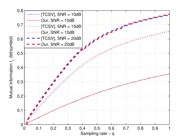
The proof of Theorem 1 is a special case of the one in [1], where the asymptotic MMSE was considered. Nonetheless, we provide in Appendix A a proof outline. Comparing Claim 1 and Theorem 1, it is seen that the results appear to be analytically quite different. Nevertheless, numerical calculations indicate that they are, in fact, equivalent. A representative comparison appears in Fig. 2.
Refer to caption

Figure 2: Mutual information rate 1subscript1{\cal I}_{1} as a function of the sampling rate q𝑞q, for SNR = 10dB, 15dB, 20dB and p=0.2𝑝0.2p=0.2.

Contrary to 1subscript1{\cal I}_{1}, the mutual information rate 2subscript2{\cal I}_{2} can be fairly easily calculated using, again, random matrix theory. Let

(x,y)=(x(1+y)2+1x(1y)2+1)2.superscript𝑥𝑦superscript𝑥superscript1𝑦21𝑥superscript1𝑦212\displaystyle{\cal F}\left(x,y\right)\stackrel{{\scriptstyle\triangle}}{{=}}\left(\sqrt{x\left(1+\sqrt{y}\right)^{2}+1}-\sqrt{x\left(1-\sqrt{y}\right)^{2}+1}\right)^{2}. (24)

The information rate 2subscript2{\cal I}_{2} is given in the following theorem.

Theorem 2

([6, Theorem 2]) The information rate 2subscript2{\cal I}_{2} is given by

2=plog[1+qσ214(qσ2,pq)]+qlog[1+pσ214(qσ2,pq)]14σ2(qσ2,pq)loge.subscript2𝑝1𝑞superscript𝜎214𝑞superscript𝜎2𝑝𝑞𝑞1𝑝superscript𝜎214𝑞superscript𝜎2𝑝𝑞14superscript𝜎2𝑞superscript𝜎2𝑝𝑞𝑒\displaystyle{\cal I}_{2}=p\log\left[1+q\sigma^{2}-\frac{1}{4}{\cal F}\left(q\sigma^{2},\frac{p}{q}\right)\right]+q\log\left[1+p\sigma^{2}-\frac{1}{4}{\cal F}\left(q\sigma^{2},\frac{p}{q}\right)\right]-\frac{1}{4\sigma^{2}}{\cal F}\left(q\sigma^{2},\frac{p}{q}\right)\log e. (25)

Equipped with closed-from expressions of 1subscript1{\cal I}_{1} and 2subscript2{\cal I}_{2}, we are now in a position to propose and explore several applications of these information rates.

IV Channel Coding

In this section, we consider three different cases that are related to channel coding problems. Generally speaking, the main differences among these cases is in the available knowledge of the transmitter and the receiver about the source. In the following applications, it is assumed that both 𝑨𝑨A and 𝑯𝑯H are available at the receiver, but are unavailable to the transmitter. Accordingly, the matrix 𝑨𝑨A𝑯𝑯H can be considered as part of the channel output, and the mutual information of interest is I(𝒀,𝑨,𝑯;𝑿)𝐼𝒀𝑨𝑯𝑿I\left(\mbox{\boldmath$Y$},\mbox{\boldmath$A$},\mbox{\boldmath$H$};\mbox{\boldmath$X$}\right). Thus, by using the chain rule of the mutual information and the fact that 𝑨𝑨A and 𝑯𝑯H are statistically independent of the source 𝑿𝑿X, we readily obtain that

I(𝒀,𝑨,𝑯;𝑿)=I(𝒀;𝑿|𝑨,𝑯),𝐼𝒀𝑨𝑯𝑿𝐼𝒀conditional𝑿𝑨𝑯\displaystyle I\left(\mbox{\boldmath$Y$},\mbox{\boldmath$A$},\mbox{\boldmath$H$};\mbox{\boldmath$X$}\right)=I\left(\mbox{\boldmath$Y$};\mbox{\boldmath$X$}|\mbox{\boldmath$A$},\mbox{\boldmath$H$}\right), (26)

and

I(𝒀,𝑨,𝑯;𝑼|𝑺)=I(𝒀;𝑼|𝑨,𝑯,𝑺),𝐼𝒀𝑨𝑯conditional𝑼𝑺𝐼𝒀conditional𝑼𝑨𝑯𝑺\displaystyle I\left(\mbox{\boldmath$Y$},\mbox{\boldmath$A$},\mbox{\boldmath$H$};\mbox{\boldmath$U$}|\mbox{\boldmath$S$}\right)=I\left(\mbox{\boldmath$Y$};\mbox{\boldmath$U$}|\mbox{\boldmath$A$},\mbox{\boldmath$H$},\mbox{\boldmath$S$}\right), (27)

which are simply identified as (8) and (9), respectively. Keeping these observations in mind, our goal is to provide achievable rates in various channel coding problems, which will only require us to know the mutual information rates 1subscript1{\cal I}_{1} and 2subscript2{\cal I}_{2}. Finally, note that part of the following coding principles have already appeared in [15], but relying on bounds.

The input 𝑿𝑿X in the previous section was considered as continuous uncoded signal. However, in the following applications, we will deal with coding problems. Accordingly, we use codes and allow the use of the channel (7) for n𝑛n times as required by the code length. The whole codebook is of size 2nRsuperscript2𝑛𝑅2^{nR} codewords. The transmitter chooses a codeword 𝑿𝑿X and transmits it over the channel.

IV-A Controlled sparsity pattern

Here, the sparsity pattern 𝑺𝑺S, as well as the Gaussian signal 𝑼𝑼U, are assumed to be controlled and given at the transmitter. The constraints are on the average support power, σ2superscript𝜎2\sigma^{2}, and the sparsity rate, that is the probability p=(Si=1)superscript𝑝subscript𝑆𝑖1p\stackrel{{\scriptstyle\triangle}}{{=}}\mathbb{P}\left(S_{i}=1\right). One motivation for this setting is, for example, in case where the transmit antennas (conveying 𝑿𝑿X) are remote, and “green" communications constraints enforce shutting off a fraction (1p)1𝑝\left(1-p\right) of the antennas, corresponding to the sparsity of the pattern 𝑺𝑺S. Here, since the shut-off pattern can be controlled, it can be used to convey information as well. We have the following immediate result.

Theorem 3 (reliable coding rate)

Assume the source-channel statistics assumptions that are given in Section II, and assume that 𝑺𝑺S and 𝑼𝑼U can be controlled by the transmitter. Then, 1subscript1{\cal I}_{1} in (23) (or in (10)) is an achievable information rate for reliable communication.

Proof 1

Since both 𝑺𝑺S and 𝑼𝑼U are controlled, then 𝑿𝑿X is also controlled. Note, however, that 𝑺𝑺S is not provided to the receiver beforehand. Thus, this is just a channel with inputs (𝑺,𝑼)𝑺𝑼\left(\mbox{\boldmath$S$},\mbox{\boldmath$U$}\right) and output 𝒀𝒀Y, where the matrices 𝑯𝑯H and 𝑨𝑨A are provided to the receiver only (the transmitter is aware of the statistics of course). Therefore, an achievable coding rate is given by (recall (26))

lim supnI(𝑺,𝑼;𝒀|𝑨,𝑯)n=lim supnI(𝑿;𝒀|𝑨,𝑯)n,subscriptlimit-supremum𝑛𝐼𝑺𝑼conditional𝒀𝑨𝑯𝑛subscriptlimit-supremum𝑛𝐼𝑿conditional𝒀𝑨𝑯𝑛\displaystyle\limsup_{n\to\infty}\frac{I\left(\mbox{\boldmath$S$},\mbox{\boldmath$U$};\mbox{\boldmath$Y$}|\mbox{\boldmath$A$},\mbox{\boldmath$H$}\right)}{n}=\limsup_{n\to\infty}\frac{I\left(\mbox{\boldmath$X$};\mbox{\boldmath$Y$}|\mbox{\boldmath$A$},\mbox{\boldmath$H$}\right)}{n}, (28)

which is exactly 1subscript1{\cal I}_{1}.

Recall that the information rate 1subscript1{\cal I}_{1}, given in Theorem 1, is valid also for sources that are not necessarily memoryless, as we allowed the model given in (3) with a general function f𝑓f. It is then interesting to check whether optimization over this class of sources can help to increase 1subscript1{\cal I}_{1}. Let

={f:[0,1](,0],f𝒜[0,1]}superscriptconditional-set𝑓formulae-sequence010𝑓𝒜01\displaystyle\mathscr{F}\stackrel{{\scriptstyle\triangle}}{{=}}\left\{f:\left[0,1\right]\to\left(-\infty,0\right],\;f\in{\cal A}\left[0,1\right]\right\} (29)

where 𝒜[0,1]𝒜01{\cal A}\left[0,1\right] is the class of analytic functions on the interval [0,1]01\left[0,1\right]. Then, according to (3), our class of sources is uniquely determined by the set of functions \mathscr{F}. Also, let fLsubscript𝑓𝐿f_{L} designate the affine function fL(m)=am+bsubscript𝑓𝐿𝑚𝑎𝑚𝑏f_{L}\left(m\right)=am+b, where a,b𝑎𝑏a,b\in\mathbb{R}, and recall that substitution of fLsubscript𝑓𝐿f_{L} in the pattern measure (3) corresponds to a memoryless assumption of the sparsity pattern. We have the following result. Finally, let 𝒫ssubscript𝒫𝑠\mathscr{P}_{s} be the set of probability distributions of the form of (3).

Theorem 4 (memoryless pattern is optimal over 𝒫ssubscript𝒫𝑠\mathscr{P}_{s})

Under the asymptotic average sparseness constraint, defined as

limn1n𝔼{i=1nSi}=p,subscript𝑛1𝑛𝔼superscriptsubscript𝑖1𝑛subscript𝑆𝑖𝑝\displaystyle\lim_{n\to\infty}\frac{1}{n}\mathbb{E}\left\{\sum_{i=1}^{n}S_{i}\right\}=p, (30)

the following holds

max𝒫s1max1=1|f=fL.subscriptsubscript𝒫𝑠subscript1subscriptsubscript1evaluated-atsubscript1𝑓subscript𝑓𝐿\displaystyle\max_{\mathscr{P}_{s}}\;{\cal I}_{1}\equiv\max_{\mathscr{F}}\;{\cal I}_{1}=\left.{\cal I}_{1}\right|_{f=f_{L}}. (31)

In words, memoryless patterns give the maximum achievable rate over 𝒫ssubscript𝒫𝑠\mathscr{P}_{s}.

Proof 2

See Appendix B

Intuitively speaking, Theorem 4 is essentially expected due to the natural symmetry in our model induced by the assumptions on 𝑨𝑨A and 𝑯𝑯H, that are given only at the receiver side (had these matrices been known to the transmitter, this result may no longer be true). Also, note that when 𝑺=(1,1,,1)𝑺111\mbox{\boldmath$S$}=\left(1,1,\ldots,1\right), namely, the source is not sparse, we obtain a MIMO setting, in which it is well-known that the Gaussian i.i.d. process achieves capacity [20]. In the following, we show that the optimal distribution of the pattern sequence must be invariant to permutations.

Theorem 5 (permutation invariant distribution)

Let 𝒮𝒮\mathscr{S} be the set of all probability distributions of 𝑺𝑺S, and let 𝒮Πsubscript𝒮Π\mathscr{S}_{\Pi} denote the set of all probability distributions that are invariant to permutations. Then,

max𝒮1=max𝒮Π1.subscript𝒮subscript1subscriptsubscript𝒮Πsubscript1\displaystyle\max_{\mathscr{S}}\;{\cal I}_{1}=\max_{\mathscr{S}_{\Pi}}\;{\cal I}_{1}. (32)
Proof 3

The maximization of I(𝒀;𝑿|𝑨,𝑯)𝐼𝒀conditional𝑿𝑨𝑯I\left(\mbox{\boldmath$Y$};\mbox{\boldmath$X$}|\mbox{\boldmath$A$},\mbox{\boldmath$H$}\right) over 𝒮𝒮\mathscr{S} boils down to the maximization of the conditional entropy H(𝒀|𝑨,𝑯)𝐻conditional𝒀𝑨𝑯H\left(\mbox{\boldmath$Y$}|\mbox{\boldmath$A$},\mbox{\boldmath$H$}\right), namely,

argmax𝒮I(𝒀;𝑿|𝑨,𝑯)subscript𝒮𝐼𝒀conditional𝑿𝑨𝑯\displaystyle\arg\max_{\mathscr{S}}\;I\left(\mbox{\boldmath$Y$};\mbox{\boldmath$X$}|\mbox{\boldmath$A$},\mbox{\boldmath$H$}\right) =argmax𝒮H(𝒀|𝑨,𝑯)absentsubscript𝒮𝐻conditional𝒀𝑨𝑯\displaystyle=\arg\max_{\mathscr{S}}\;H\left(\mbox{\boldmath$Y$}|\mbox{\boldmath$A$},\mbox{\boldmath$H$}\right) (33)
=argmax𝒮𝔼[log1(𝒀|𝑨,𝑯)].absentsubscript𝒮𝔼delimited-[]1conditional𝒀𝑨𝑯\displaystyle=\arg\max_{\mathscr{S}}\;\mathbb{E}\left[\log\frac{1}{\mathbb{P}\left(\mbox{\boldmath$Y$}|\mbox{\boldmath$A$},\mbox{\boldmath$H$}\right)}\right]. (34)

Recall that

(𝒀|𝑨,𝑯)=nd𝒙(𝒙)(𝒀|𝑨,𝑯,𝒙).conditional𝒀𝑨𝑯subscriptsuperscript𝑛differential-d𝒙𝒙conditional𝒀𝑨𝑯𝒙\displaystyle\mathbb{P}\left(\mbox{\boldmath$Y$}|\mbox{\boldmath$A$},\mbox{\boldmath$H$}\right)=\int_{\mathbb{R}^{n}}\mathrm{d}\mbox{\boldmath$x$}\mathbb{P}\left(\mbox{\boldmath$x$}\right)\mathbb{P}\left(\mbox{\boldmath$Y$}|\mbox{\boldmath$A$},\mbox{\boldmath$H$},\mbox{\boldmath$x$}\right). (35)

Since the columns of 𝑨𝑨A𝑯𝑯H are i.i.d. and (𝑨,𝑯)𝑨𝑯\left(\mbox{\boldmath$A$},\mbox{\boldmath$H$}\right) are known solely to the receiver, it is evident that the conditional entropy H(𝒀|𝑨,𝑯)𝐻conditional𝒀𝑨𝑯H\left(\mbox{\boldmath$Y$}|\mbox{\boldmath$A$},\mbox{\boldmath$H$}\right) is invariant to permutations of 𝑺𝑺S in (𝑺)𝑺\mathbb{P}\left(\mbox{\boldmath$S$}\right). To see this, let π(𝑺)subscript𝜋𝑺\mathbb{P}_{\pi}\left(\mbox{\boldmath$S$}\right) denote some permuted version of (𝑺)𝑺\mathbb{P}\left(\mbox{\boldmath$S$}\right), namely, π(𝑺)=(𝚷𝑺)subscript𝜋𝑺𝚷𝑺\mathbb{P}_{\pi}\left(\mbox{\boldmath$S$}\right)=\mathbb{P}\left({\mbox{\boldmath$\Pi$}}\mbox{\boldmath$S$}\right) where 𝚷𝚷\Pi is a permutation matrix corresponding to some permutation. Accordingly, let π(𝑿)subscript𝜋𝑿\mathbb{P}_{\pi}\left(\mbox{\boldmath$X$}\right) be the probability distribution of 𝑿𝑿X induced by the permuted distribution π(𝑺)subscript𝜋𝑺\mathbb{P}_{\pi}\left(\mbox{\boldmath$S$}\right). Finally, let Hπ(𝒀|𝑨,𝑯)subscript𝐻𝜋conditional𝒀𝑨𝑯H_{\pi}\left(\mbox{\boldmath$Y$}|\mbox{\boldmath$A$},\mbox{\boldmath$H$}\right) designate the conditional entropy of 𝒀𝒀Y given (𝑨,𝑯)𝑨𝑯\left(\mbox{\boldmath$A$},\mbox{\boldmath$H$}\right) where 𝑿𝑿X is distributed according to π(𝑿)subscript𝜋𝑿\mathbb{P}_{\pi}\left(\mbox{\boldmath$X$}\right). Then,

Hπ(𝒀|𝑨,𝑯)subscript𝐻𝜋conditional𝒀𝑨𝑯\displaystyle H_{\pi}\left(\mbox{\boldmath$Y$}|\mbox{\boldmath$A$},\mbox{\boldmath$H$}\right) =𝔼{lognd𝒙π(𝒙)(𝒀|𝑨,𝑯,𝒙)}absent𝔼subscriptsuperscript𝑛differential-d𝒙subscript𝜋𝒙conditional𝒀𝑨𝑯𝒙\displaystyle=-\mathbb{E}\left\{\log\int_{\mathbb{R}^{n}}\mathrm{d}\mbox{\boldmath$x$}\mathbb{P}_{\pi}\left(\mbox{\boldmath$x$}\right)\mathbb{P}\left(\mbox{\boldmath$Y$}|\mbox{\boldmath$A$},\mbox{\boldmath$H$},\mbox{\boldmath$x$}\right)\right\} (36)
=𝔼{lognd𝒙π(𝚷𝒙)(𝒀|𝑨,𝑯,𝚷𝒙)}absent𝔼subscriptsuperscript𝑛differential-d𝒙subscript𝜋𝚷𝒙conditional𝒀𝑨𝑯𝚷𝒙\displaystyle=-\mathbb{E}\left\{\log\int_{\mathbb{R}^{n}}\mathrm{d}\mbox{\boldmath$x$}\mathbb{P}_{\pi}\left({\mbox{\boldmath$\Pi$}}\mbox{\boldmath$x$}\right)\mathbb{P}\left(\mbox{\boldmath$Y$}|\mbox{\boldmath$A$},\mbox{\boldmath$H$},{\mbox{\boldmath$\Pi$}}\mbox{\boldmath$x$}\right)\right\} (37)
=𝔼{lognd𝒙(𝒙)(𝒀|𝑨,𝑯,𝚷𝒙)}absent𝔼subscriptsuperscript𝑛differential-d𝒙𝒙conditional𝒀𝑨𝑯𝚷𝒙\displaystyle=-\mathbb{E}\left\{\log\int_{\mathbb{R}^{n}}\mathrm{d}\mbox{\boldmath$x$}\mathbb{P}\left(\mbox{\boldmath$x$}\right)\mathbb{P}\left(\mbox{\boldmath$Y$}|\mbox{\boldmath$A$},\mbox{\boldmath$H$},{\mbox{\boldmath$\Pi$}}\mbox{\boldmath$x$}\right)\right\} (38)

where in the second equality we changed the variable 𝒙𝚷𝒙maps-to𝒙𝚷𝒙\mbox{\boldmath$x$}\mapsto{\mbox{\boldmath$\Pi$}}\mbox{\boldmath$x$} which permutes the vector 𝒙𝒙x according to the permutation used in π(𝑺)subscript𝜋𝑺\mathbb{P}_{\pi}\left(\mbox{\boldmath$S$}\right). Now,

Hπ(𝒀|𝑨,𝑯)=𝔼{logn1(2π)k/2d𝒙(𝒙)exp(12𝒀𝑨𝑯𝚷𝒙2)}subscript𝐻𝜋conditional𝒀𝑨𝑯𝔼subscriptsuperscript𝑛1superscript2𝜋𝑘2differential-d𝒙𝒙12superscriptnorm𝒀𝑨𝑯𝚷𝒙2\displaystyle H_{\pi}\left(\mbox{\boldmath$Y$}|\mbox{\boldmath$A$},\mbox{\boldmath$H$}\right)=-\mathbb{E}\left\{\log\int_{\mathbb{R}^{n}}\frac{1}{\left(2\pi\right)^{k/2}}\mathrm{d}\mbox{\boldmath$x$}\mathbb{P}\left(\mbox{\boldmath$x$}\right)\exp\left(-\frac{1}{2}\left\|\mbox{\boldmath$Y$}-\mbox{\boldmath$A$}\mbox{\boldmath$H$}{\mbox{\boldmath$\Pi$}}\mbox{\boldmath$x$}\right\|^{2}\right)\right\} (39)
=d(𝒚|𝑨,𝑯)d(𝑨,𝑯)[logn1(2π)k/2d𝒙(𝒙)exp(12𝒚𝑨𝑯𝚷𝒙2)]absentdifferential-dconditional𝒚𝑨𝑯differential-d𝑨𝑯delimited-[]subscriptsuperscript𝑛1superscript2𝜋𝑘2differential-d𝒙𝒙12superscriptnorm𝒚𝑨𝑯𝚷𝒙2\displaystyle=-\int\mathrm{d}\mathbb{P}\left(\mbox{\boldmath$y$}|\mbox{\boldmath$A$},\mbox{\boldmath$H$}\right)\mathrm{d}\mathbb{P}\left(\mbox{\boldmath$A$},\mbox{\boldmath$H$}\right)\left[\log\int_{\mathbb{R}^{n}}\frac{1}{\left(2\pi\right)^{k/2}}\mathrm{d}\mbox{\boldmath$x$}\mathbb{P}\left(\mbox{\boldmath$x$}\right)\exp\left(-\frac{1}{2}\left\|\mbox{\boldmath$y$}-\mbox{\boldmath$A$}\mbox{\boldmath$H$}{\mbox{\boldmath$\Pi$}}\mbox{\boldmath$x$}\right\|^{2}\right)\right] (40)
=d(𝒚|𝑨,𝑯𝚷T)d(𝑨,𝑯𝚷T)[logn1(2π)k/2d𝒙(𝒙)exp(12𝒚𝑨(𝑯𝚷T)𝚷𝒙2)]absentdifferential-dconditional𝒚𝑨superscript𝑯𝚷𝑇differential-d𝑨superscript𝑯𝚷𝑇delimited-[]subscriptsuperscript𝑛1superscript2𝜋𝑘2differential-d𝒙𝒙12superscriptnorm𝒚𝑨superscript𝑯𝚷𝑇𝚷𝒙2\displaystyle=-\int\mathrm{d}\mathbb{P}\left(\mbox{\boldmath$y$}|\mbox{\boldmath$A$},\mbox{\boldmath$H$}{\mbox{\boldmath$\Pi$}}^{T}\right)\mathrm{d}\mathbb{P}\left(\mbox{\boldmath$A$},\mbox{\boldmath$H$}{\mbox{\boldmath$\Pi$}}^{T}\right)\left[\log\int_{\mathbb{R}^{n}}\frac{1}{\left(2\pi\right)^{k/2}}\mathrm{d}\mbox{\boldmath$x$}\mathbb{P}\left(\mbox{\boldmath$x$}\right)\exp\left(-\frac{1}{2}\left\|\mbox{\boldmath$y$}-\mbox{\boldmath$A$}(\mbox{\boldmath$H$}{\mbox{\boldmath$\Pi$}}^{T}){\mbox{\boldmath$\Pi$}}\mbox{\boldmath$x$}\right\|^{2}\right)\right] (41)
=d(𝒚|𝑨,𝑯)d(𝑨,𝑯)[logn1(2π)k/2d𝒙(𝒙)exp(12𝒚𝑨𝑯𝒙2)]absentdifferential-dconditional𝒚𝑨𝑯differential-d𝑨𝑯delimited-[]subscriptsuperscript𝑛1superscript2𝜋𝑘2differential-d𝒙𝒙12superscriptnorm𝒚𝑨𝑯𝒙2\displaystyle=-\int\mathrm{d}\mathbb{P}\left(\mbox{\boldmath$y$}|\mbox{\boldmath$A$},\mbox{\boldmath$H$}\right)\mathrm{d}\mathbb{P}\left(\mbox{\boldmath$A$},\mbox{\boldmath$H$}\right)\left[\log\int_{\mathbb{R}^{n}}\frac{1}{\left(2\pi\right)^{k/2}}\mathrm{d}\mbox{\boldmath$x$}\mathbb{P}\left(\mbox{\boldmath$x$}\right)\exp\left(-\frac{1}{2}\left\|\mbox{\boldmath$y$}-\mbox{\boldmath$A$}\mbox{\boldmath$H$}\mbox{\boldmath$x$}\right\|^{2}\right)\right] (42)
=H(𝒀|𝑨,𝑯)absent𝐻conditional𝒀𝑨𝑯\displaystyle=H\left(\mbox{\boldmath$Y$}|\mbox{\boldmath$A$},\mbox{\boldmath$H$}\right) (43)

where in the third equality we changed the variable 𝑯𝑯𝚷Tmaps-to𝑯superscript𝑯𝚷𝑇\mbox{\boldmath$H$}\mapsto\mbox{\boldmath$H$}{\mbox{\boldmath$\Pi$}}^{T}, and the forth equality follows from the facts that 𝑯𝚷T𝚷𝒙=𝑯𝒙superscript𝑯𝚷𝑇𝚷𝒙𝑯𝒙\mbox{\boldmath$H$}{\mbox{\boldmath$\Pi$}}^{T}{\mbox{\boldmath$\Pi$}}\mbox{\boldmath$x$}=\mbox{\boldmath$H$}\mbox{\boldmath$x$} and that (𝑨,𝑯)𝑨𝑯\left(\mbox{\boldmath$A$},\mbox{\boldmath$H$}\right) are i.i.d. and thus (𝑨,𝑯𝚷T)=(𝑨,𝑯)𝑨superscript𝑯𝚷𝑇𝑨𝑯\mathbb{P}\left(\mbox{\boldmath$A$},\mbox{\boldmath$H$}{\mbox{\boldmath$\Pi$}}^{T}\right)=\mathbb{P}\left(\mbox{\boldmath$A$},\mbox{\boldmath$H$}\right).

Continuing, let 𝒮subscript𝒮\mathbb{P}_{*}\in\mathscr{S} denote the probability distribution that maximize I(𝒀;𝑿|𝑨,𝑯)𝐼𝒀conditional𝑿𝑨𝑯I\left(\mbox{\boldmath$Y$};\mbox{\boldmath$X$}|\mbox{\boldmath$A$},\mbox{\boldmath$H$}\right). Let ΠsubscriptΠ\Pi_{*} denote the set of probability distributions obtained from subscript\mathbb{P}_{*} by all possible permutations of 𝑺𝑺S, and thus each is achieving the maximal I(𝒀;𝑿|𝑨,𝑯)𝐼𝒀conditional𝑿𝑨𝑯I\left(\mbox{\boldmath$Y$};\mbox{\boldmath$X$}|\mbox{\boldmath$A$},\mbox{\boldmath$H$}\right). Also, let

inv(𝑺)=1|Π|Π(𝑺).superscriptsubscriptinv𝑺1subscriptΠsubscriptsubscriptΠ𝑺\displaystyle\mathbb{P}_{\text{inv}}\left(\mbox{\boldmath$S$}\right)\stackrel{{\scriptstyle\triangle}}{{=}}\frac{1}{\left|\Pi_{*}\right|}\sum_{\mathbb{P}\in\Pi_{*}}\mathbb{P}\left(\mbox{\boldmath$S$}\right). (44)

Note that inv(𝑺)𝒮Πsubscriptinv𝑺subscript𝒮Π\mathbb{P}_{\text{inv}}\left(\mbox{\boldmath$S$}\right)\in\mathscr{S}_{\Pi}, namely, inv(𝑺)subscriptinv𝑺\mathbb{P}_{\text{inv}}\left(\mbox{\boldmath$S$}\right) is invariant to permutations. Finally, let H(𝒀|𝑨,𝑯)|invevaluated-at𝐻conditional𝒀𝑨𝑯subscriptinvH\left(\mbox{\boldmath$Y$}|\mbox{\boldmath$A$},\mbox{\boldmath$H$}\right)|_{\mathbb{P}_{\text{inv}}} and H(𝒀|𝑨,𝑯)|evaluated-at𝐻conditional𝒀𝑨𝑯subscriptH\left(\mbox{\boldmath$Y$}|\mbox{\boldmath$A$},\mbox{\boldmath$H$}\right)|_{\mathbb{P}_{*}} designate the conditional entropies of 𝒀𝒀Y given (𝑨,𝑯)𝑨𝑯\left(\mbox{\boldmath$A$},\mbox{\boldmath$H$}\right) where 𝑺𝑺S is distributed according to invsubscriptinv\mathbb{P}_{\text{inv}} and subscript\mathbb{P}_{*}, respectively. Thus, from the concavity of H(𝒀|𝑨,𝑯)𝐻conditional𝒀𝑨𝑯H\left(\mbox{\boldmath$Y$}|\mbox{\boldmath$A$},\mbox{\boldmath$H$}\right) w.r.t. (|𝑨,𝑯)\mathbb{P}\left(\cdot|\mbox{\boldmath$A$},\mbox{\boldmath$H$}\right), we have that

H(𝒀|𝑨,𝑯)|invevaluated-at𝐻conditional𝒀𝑨𝑯subscriptinv\displaystyle H\left(\mbox{\boldmath$Y$}|\mbox{\boldmath$A$},\mbox{\boldmath$H$}\right)|_{\mathbb{P}_{\text{inv}}} =𝔼{log𝒔{0,1}nπ(𝑺)(𝒀|𝑨,𝑯,𝑺)}superscriptabsent𝔼subscript𝒔superscript01𝑛subscript𝜋𝑺conditional𝒀𝑨𝑯𝑺\displaystyle\stackrel{{\scriptstyle\triangle}}{{=}}-\mathbb{E}\left\{\log\sum_{\mbox{\footnotesize\boldmath$s$}\in\left\{0,1\right\}^{n}}\mathbb{P}_{\pi}\left(\mbox{\boldmath$S$}\right)\mathbb{P}\left(\mbox{\boldmath$Y$}|\mbox{\boldmath$A$},\mbox{\boldmath$H$},\mbox{\boldmath$S$}\right)\right\} (45)
1|Π|Π𝔼{log𝒔{0,1}n(𝑺)(𝒀|𝑨,𝑯,𝑺)}absent1subscriptΠsubscriptsubscriptΠ𝔼subscript𝒔superscript01𝑛𝑺conditional𝒀𝑨𝑯𝑺\displaystyle\geq-\frac{1}{\left|\Pi_{*}\right|}\sum_{\mathbb{P}\in\Pi_{*}}\mathbb{E}\left\{\log\sum_{\mbox{\footnotesize\boldmath$s$}\in\left\{0,1\right\}^{n}}\mathbb{P}\left(\mbox{\boldmath$S$}\right)\mathbb{P}\left(\mbox{\boldmath$Y$}|\mbox{\boldmath$A$},\mbox{\boldmath$H$},\mbox{\boldmath$S$}\right)\right\} (46)
=H(𝒀|𝑨,𝑯)|absentevaluated-at𝐻conditional𝒀𝑨𝑯subscript\displaystyle=H\left(\mbox{\boldmath$Y$}|\mbox{\boldmath$A$},\mbox{\boldmath$H$}\right)|_{\mathbb{P}_{*}} (47)

where (47) follows from the fact that the conditional entropy is the same for all members of ΠsubscriptΠ\Pi_{*} as was mentioned previously.

It is tempting to tie Theorems 4 and 5 to infer that the optimal distribution of 𝑺𝑺S over 𝒮𝒮\mathscr{S} is memoryless. However, there is still a little gap. Indeed, despite the fact that permutation invariant distributions must depend on the pattern only through the magnetization, not every such distribution can be expressed as the one in (3), due to the smoothness requirement of f𝑓f. For example, in case of uniform distributions over types, the function f𝑓f is not continuous. Nonetheless, roughly speaking, it is evident that one can approximate arbitrarily closely such non-smooth behaviors by a respectively smooth function f𝑓f. So, we conjecture that the maximum mutual information is indeed achieved by a memoryless source.

Finally, we present in Fig. 3 the mutual information rate 1subscript1{\cal I}_{1} as a function of the sampling rate q𝑞q and the SNR for p=0.2𝑝0.2p=0.2. It can be seen that increase of the rate or/and the SNR results in an increase of 1subscript1{\cal I}_{1}, as one should expect.

Refer to caption

Figure 3: Mutual information rate 1subscript1{\cal I}_{1} as a function of q𝑞q and the SNR for p=0.2𝑝0.2p=0.2.

IV-B Unknown sparsity pattern

In this subsection, we consider the case where the sparsity pattern is unknown to all parties. The vector 𝑼𝑼U is treated as the information to be transmitted over the channel.

(𝑺)𝑺\mathbb{P}(\mbox{\boldmath$S$})𝑿(𝑼,𝑺)𝑿𝑼𝑺\mbox{\boldmath$X$}\left(\mbox{\boldmath$U$},\mbox{\boldmath$S$}\right)𝑼𝑼U𝒀𝒀Y(𝒀|𝑿,𝑨,𝑯)conditional𝒀𝑿𝑨𝑯\mathbb{P}(\mbox{\boldmath$Y$}|\mbox{\boldmath$X$},\mbox{\boldmath$A$},\mbox{\boldmath$H$})𝑿𝑿X
Figure 4: Gel’fand-Pinsker channel.

In this setting, we have the following result.

Theorem 6 (unknown sparsity pattern)

The channel (|𝑿,𝑨,𝑯)\mathbb{P}\left(\cdot|\mbox{\boldmath$X$},\mbox{\boldmath$A$},\mbox{\boldmath$H$}\right), defined in Section II, has an achievable rate given by

R=12(ma).𝑅subscript1subscript2subscript𝑚𝑎\displaystyle R={\cal I}_{1}-{\cal H}_{2}\left(m_{a}\right). (48)
Proof 4

This is a channel with input 𝑼𝑼U and output 𝒀𝒀Y, where the matrices 𝑨𝑨A and 𝑯𝑯H are known only to the receiver. Therefore,

I(𝑼;𝒀|𝑨,𝑯,𝑺)𝐼𝑼conditional𝒀𝑨𝑯𝑺\displaystyle I\left(\mbox{\boldmath$U$};\mbox{\boldmath$Y$}|\mbox{\boldmath$A$},\mbox{\boldmath$H$},\mbox{\boldmath$S$}\right) I(𝑼;𝒀|𝑨,𝑯)absent𝐼𝑼conditional𝒀𝑨𝑯\displaystyle\geq I\left(\mbox{\boldmath$U$};\mbox{\boldmath$Y$}|\mbox{\boldmath$A$},\mbox{\boldmath$H$}\right) (49)
=I(𝑼,𝑺;𝒀|𝑨,𝑯)I(𝑺;𝒀|𝑼,𝑨,𝑯)absent𝐼𝑼𝑺conditional𝒀𝑨𝑯𝐼𝑺conditional𝒀𝑼𝑨𝑯\displaystyle=I\left(\mbox{\boldmath$U$},\mbox{\boldmath$S$};\mbox{\boldmath$Y$}|\mbox{\boldmath$A$},\mbox{\boldmath$H$}\right)-I\left(\mbox{\boldmath$S$};\mbox{\boldmath$Y$}|\mbox{\boldmath$U$},\mbox{\boldmath$A$},\mbox{\boldmath$H$}\right) (50)
I(𝑿;𝒀|𝑨,𝑯)H(𝑺),absent𝐼𝑿conditional𝒀𝑨𝑯𝐻𝑺\displaystyle\geq I\left(\mbox{\boldmath$X$};\mbox{\boldmath$Y$}|\mbox{\boldmath$A$},\mbox{\boldmath$H$}\right)-H(\mbox{\boldmath$S$}), (51)

and the result follow, after normalizing by n𝑛n and taking the limit n𝑛n\to\infty.

Yet another interesting setting is the case in which the transmitter cannot control the sparsity pattern that is given beforehand. This pattern, 𝑺𝑺S, is considered to be channel state available non-causally/causally to the transmitter solely. The vector 𝑼𝑼U is treated as the information to be transmitted over the channel. This framework falls within the well-known Gel’fand-Pinsker channel [18] and the Shannon settings [17], for non-causal and causal knowledge of 𝑺𝑺S, respectively. This is illustrated in Fig. 4. A possible motivation for this setting is when the transmitter, that produces the input 𝑼𝑼U, knows the pattern of switched antennas/shut-off pattern (“green" wireless), but cannot control it. In the following, customary to the Gel’fand-Pinsker and the Shannon settings, the channel state is assumed an i.i.d. process such that p=(Si=1)superscript𝑝subscript𝑆𝑖1p\stackrel{{\scriptstyle\triangle}}{{=}}\mathbb{P}\left(S_{i}=1\right).

For the case where the side information is available at the transmitter only causally, the capacity expression has been found by Shannon in [17], and is given by

max(𝒗),𝒖(𝒗,𝒔)I(𝑽;𝒀|𝑨,𝑯)subscript𝒗𝒖𝒗𝒔𝐼𝑽conditional𝒀𝑨𝑯\displaystyle\max_{\mathbb{P}\left(\mbox{\footnotesize\boldmath$v$}\right),\mbox{\footnotesize\boldmath$u$}\left(\mbox{\footnotesize\boldmath$v$},\mbox{\footnotesize\boldmath$s$}\right)}\;I\left(\mbox{\boldmath$V$};\mbox{\boldmath$Y$}|\mbox{\boldmath$A$},\mbox{\boldmath$H$}\right) (52)

where 𝑼(𝑽,𝑺)𝑼𝑽𝑺\mbox{\boldmath$U$}\left(\mbox{\boldmath$V$},\mbox{\boldmath$S$}\right) is a deterministic function of 𝑽𝑽V and 𝑺𝑺S. Note that the auxiliary 𝑽𝑽V should be chosen independently of the state [21], while the transmitted signal can depend on the state. Now, since the sparsity pattern is given, we can adapt the power of the transmitted signal accordingly, that is, we do not transmit at times when Si=0subscript𝑆𝑖0S_{i}=0. Accordingly, let us choose 𝑽=𝑼𝑽superscript𝑼\mbox{\boldmath$V$}=\mbox{\boldmath$U$}^{\prime}, where 𝑼superscript𝑼\mbox{\boldmath$U$}^{\prime} is a Gaussian random vector with independent elements, each with zero mean and variance p1σ2superscript𝑝1superscript𝜎2p^{-1}\sigma^{2}. The transmitted signal is 𝑼=𝑺𝑽𝑼direct-product𝑺𝑽\mbox{\boldmath$U$}=\mbox{\boldmath$S$}\odot\mbox{\boldmath$V$} (which maintains the average power constraint), where direct-product\odot denotes the Hadamard product, and thus 𝑿=𝑺𝑼=𝑺𝑽𝑿direct-product𝑺𝑼direct-product𝑺𝑽\mbox{\boldmath$X$}=\mbox{\boldmath$S$}\odot\mbox{\boldmath$U$}=\mbox{\boldmath$S$}\odot\mbox{\boldmath$V$}, where we have used the fact that 𝑺𝑺=𝑺direct-product𝑺𝑺𝑺\mbox{\boldmath$S$}\odot\mbox{\boldmath$S$}=\mbox{\boldmath$S$}. Therefore, (52) reads

I(𝑽;𝒀|𝑨,𝑯)=I(𝑼;𝒀|𝑨,𝑯).𝐼𝑽conditional𝒀𝑨𝑯𝐼superscript𝑼conditional𝒀𝑨𝑯\displaystyle I\left(\mbox{\boldmath$V$};\mbox{\boldmath$Y$}|\mbox{\boldmath$A$},\mbox{\boldmath$H$}\right)=I\left(\mbox{\boldmath$U$}^{\prime};\mbox{\boldmath$Y$}|\mbox{\boldmath$A$},\mbox{\boldmath$H$}\right). (53)

Unfortunately, we were unable to derive a closed-from expression for the information rate corresponding to I(𝑼;𝒀|𝑨,𝑯)𝐼superscript𝑼conditional𝒀𝑨𝑯I\left(\mbox{\boldmath$U$}^{\prime};\mbox{\boldmath$Y$}|\mbox{\boldmath$A$},\mbox{\boldmath$H$}\right). Nonetheless, we note that

I(𝑼;𝒀|𝑨,𝑯)𝐼superscript𝑼conditional𝒀𝑨𝑯\displaystyle I\left(\mbox{\boldmath$U$}^{\prime};\mbox{\boldmath$Y$}|\mbox{\boldmath$A$},\mbox{\boldmath$H$}\right) =I(𝑼,𝑺;𝒀|𝑨,𝑯)I(𝑺;𝒀|𝑼,𝑨,𝑯)absent𝐼superscript𝑼𝑺conditional𝒀𝑨𝑯𝐼𝑺conditional𝒀superscript𝑼𝑨𝑯\displaystyle=I\left(\mbox{\boldmath$U$}^{\prime},\mbox{\boldmath$S$};\mbox{\boldmath$Y$}|\mbox{\boldmath$A$},\mbox{\boldmath$H$}\right)-I\left(\mbox{\boldmath$S$};\mbox{\boldmath$Y$}|\mbox{\boldmath$U$}^{\prime},\mbox{\boldmath$A$},\mbox{\boldmath$H$}\right) (54)
=I(𝑿;𝒀|𝑨,𝑯)I(𝑺;𝒀|𝑨,𝑯)absent𝐼𝑿conditional𝒀𝑨𝑯𝐼𝑺conditional𝒀𝑨𝑯\displaystyle=I\left(\mbox{\boldmath$X$};\mbox{\boldmath$Y$}|\mbox{\boldmath$A$},\mbox{\boldmath$H$}\right)-I\left(\mbox{\boldmath$S$};\mbox{\boldmath$Y$}|\mbox{\boldmath$A$},\mbox{\boldmath$H$}\right) (55)
I(𝑿;𝒀|𝑨,𝑯)H(𝑺).absent𝐼𝑿conditional𝒀𝑨𝑯𝐻𝑺\displaystyle\geq I\left(\mbox{\boldmath$X$};\mbox{\boldmath$Y$}|\mbox{\boldmath$A$},\mbox{\boldmath$H$}\right)-H\left(\mbox{\boldmath$S$}\right). (56)

Accordingly, the achievable rate is given by 1,S2(p)subscript1𝑆subscript2𝑝{\cal I}_{1,S}-{\cal H}_{2}\left(p\right), where 1,Ssubscript1𝑆{\cal I}_{1,S} is given in (10) with σ2superscript𝜎2\sigma^{2} replaced by p1σ2superscript𝑝1superscript𝜎2p^{-1}\sigma^{2}, that is the overall SNR is scaled from pσ2𝑝superscript𝜎2p\sigma^{2} to σ2superscript𝜎2\sigma^{2}. Thus, the improvement due to the knowledge of 𝑺𝑺S at the transmitter side compared to Theorem 6 is evident. For the non-causal case, namely, the Gel’fand-Pinsker channel, we could not find a good choice for the auxiliary variable 𝑽𝑽V. In [22], the related case of fading (which may be binary) given as side information known to the transmitter only was considered.

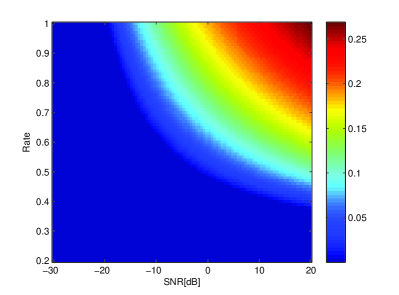
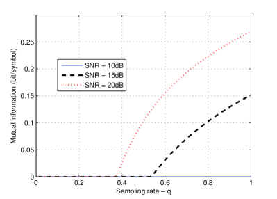
Theorems 3 and 6 demonstrate how important it is to be able to control the sparsity pattern 𝑺𝑺S. Indeed, it can be seen that the gap between these two achievable rates is exactly 2(p)subscript2𝑝{\cal H}_{2}\left(p\right) which quantifies our uncertainty at the receiver regarding the source support. This is illustrated in Fig. 5, which shows the achievable rate as a function of q𝑞q and the SNR, for p=0.2𝑝0.2p=0.2. It can be seen that there is a significant region of rates and SNR’s for which the achievable rate is zero (within this region, the subtractive term in (48) dominates). This is attributed to the fact that the sparsity pattern is uncontrolled, and can be interpreted as the overhead required to the transmitter to adapt to the channel state.
Refer to caption
(a)
Refer to caption
(b)
Figure 5: Achievable rate in the uncontrolled sparsity pattern case, as a function of q𝑞q and the SNR, for p=0.2𝑝0.2p=0.2.

IV-C The sparsity pattern is carrying the information

In this subsection, we consider the case where the information is conveyed via 𝑺𝑺S, while 𝑼𝑼U plays the role of a fading process, known to nobody. In this case, we have the following result.

Theorem 7 (informative sparsity pattern)

Consider the case in which 𝑺𝑺S is carrying the information and 𝑼𝑼U is unknown both to the receiver and the transmitter. Then, the achievable rate is given by R=12𝑅subscript1subscript2R={\cal I}_{1}-{\cal I}_{2}.

Proof 5

Evidently, under the theorem settings, what matters is the mutual information I(𝑺;𝒀|𝑨,𝑯)𝐼𝑺conditional𝒀𝑨𝑯I\left(\mbox{\boldmath$S$};\mbox{\boldmath$Y$}|\mbox{\boldmath$A$},\mbox{\boldmath$H$}\right) which readily can be expressed as

I(𝑺;𝒀|𝑨,𝑯)𝐼𝑺conditional𝒀𝑨𝑯\displaystyle I\left(\mbox{\boldmath$S$};\mbox{\boldmath$Y$}|\mbox{\boldmath$A$},\mbox{\boldmath$H$}\right) =I(𝒀;𝑼,𝑺|𝑨,𝑯)I(𝒀;𝑼|𝑨,𝑯,𝑺)absent𝐼𝒀𝑼conditional𝑺𝑨𝑯𝐼𝒀conditional𝑼𝑨𝑯𝑺\displaystyle=I\left(\mbox{\boldmath$Y$};\mbox{\boldmath$U$},\mbox{\boldmath$S$}|\mbox{\boldmath$A$},\mbox{\boldmath$H$}\right)-I\left(\mbox{\boldmath$Y$};\mbox{\boldmath$U$}|\mbox{\boldmath$A$},\mbox{\boldmath$H$},\mbox{\boldmath$S$}\right) (57)
=I(𝒀;𝑼,𝑺|𝑨,𝑯)I(𝒀;𝑼|𝑨,𝑯,𝑺)absent𝐼𝒀𝑼conditional𝑺𝑨𝑯𝐼𝒀conditional𝑼𝑨𝑯𝑺\displaystyle=I\left(\mbox{\boldmath$Y$};\mbox{\boldmath$U$},\mbox{\boldmath$S$}|\mbox{\boldmath$A$},\mbox{\boldmath$H$}\right)-I\left(\mbox{\boldmath$Y$};\mbox{\boldmath$U$}|\mbox{\boldmath$A$},\mbox{\boldmath$H$},\mbox{\boldmath$S$}\right) (58)
=I(𝒀;𝑿|𝑨,𝑯)I(𝒀;𝑼|𝑨,𝑯,𝑺),absent𝐼𝒀conditional𝑿𝑨𝑯𝐼𝒀conditional𝑼𝑨𝑯𝑺\displaystyle=I\left(\mbox{\boldmath$Y$};\mbox{\boldmath$X$}|\mbox{\boldmath$A$},\mbox{\boldmath$H$}\right)-I\left(\mbox{\boldmath$Y$};\mbox{\boldmath$U$}|\mbox{\boldmath$A$},\mbox{\boldmath$H$},\mbox{\boldmath$S$}\right), (59)

and thus Theorem 7 follows, after normalizing by n𝑛n and taking the limit n𝑛n\to\infty.

Note that similarly to Subsection IV-A, an optimization over the input distribution can be considered. Nonetheless, by using the same arguments it can be shown that there is no gain by using sources with memory. In the following, we consider the high SNR regime. It is not difficult to show that for large σ2superscript𝜎2\sigma^{2}, the behavior of 2subscript2{\cal I}_{2} is as follows [6, Eq. (34)]

2=min{q,p}log(1+4min{q,p}σ2)+𝒪(1)subscript2𝑞𝑝14𝑞𝑝superscript𝜎2𝒪1\displaystyle{\cal I}_{2}=\min\left\{q,p\right\}\log\left(1+4\min\left\{q,p\right\}\sigma^{2}\right)+{\cal O}\left(1\right) (60)

Note that the prelog constant (a.k.a. the degree of freedom) in the above term of 2subscript2{\cal I}_{2} is just the asymptotic almost-sure rank of the matrix 𝑨𝑨A𝑯𝑯H𝑺𝑺S, as one should expect. Similarly, the prelog of 1subscript1{\cal I}_{1} is also min{q,p}𝑞𝑝\min\left\{q,p\right\}. Thus, if we let

=limnI(𝑺;𝒀|𝑨,𝑯)n,superscriptsubscript𝑛𝐼𝑺conditional𝒀𝑨𝑯𝑛\displaystyle{\cal I}\stackrel{{\scriptstyle\triangle}}{{=}}\lim_{n\to\infty}\frac{I\left(\mbox{\boldmath$S$};\mbox{\boldmath$Y$}|\mbox{\boldmath$A$},\mbox{\boldmath$H$}\right)}{n}, (61)

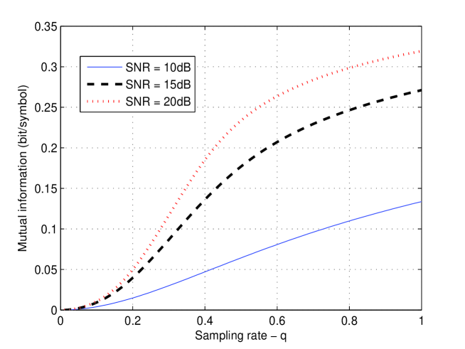
then following the last observations regarding the prelogs of 1subscript1{\cal I}_{1} and 2subscript2{\cal I}_{2}, it can be seen that the information rate {\cal I} converges in the high SNR regime to a finite value that is independent of σ2superscript𝜎2\sigma^{2}. This is not surprising due to the obvious fact that 2(p)subscript2𝑝{\cal I}\leq{\cal H}_{2}\left(p\right). Fig. 6 shows the achievable rate for p=0.2𝑝0.2p=0.2. It is evident that due to the fading induced by 𝑼𝑼U, there is a significant decrease in the achievable rate.
Refer to caption

Figure 6: Achievable rate when the sparsity pattern is carrying the information, as a function of q𝑞q and the SNR, for p=0.2𝑝0.2p=0.2.

V The Wiretap Channel

In the wiretap channel [23], symbols that are transmitted through a main channel to a legitimate receiver are observed by an eavesdropper across a wiretap channel. The goal of coding for wiretap channels is to facilitate error-free decoding across the main channel, while ensuring that the information transfer rate across the wiretap channel would be as small as possible. A desirable property here is weak secrecy, which means that the normalized mutual information between the source and the wiretap channel output will tend to zero.

In our problem, we consider the case in which the legitimate user receives

𝒀1=𝑨1𝑯1𝑿+𝑾1,subscript𝒀1subscript𝑨1subscript𝑯1𝑿subscript𝑾1\displaystyle\mbox{\boldmath$Y$}_{1}=\mbox{\boldmath$A$}_{1}\mbox{\boldmath$H$}_{1}\mbox{\boldmath$X$}+\mbox{\boldmath$W$}_{1}, (62)

while the eavesdropper receives

𝒀2=𝑨2𝑯2𝑿+𝑾2.subscript𝒀2subscript𝑨2subscript𝑯2𝑿subscript𝑾2\displaystyle\mbox{\boldmath$Y$}_{2}=\mbox{\boldmath$A$}_{2}\mbox{\boldmath$H$}_{2}\mbox{\boldmath$X$}+\mbox{\boldmath$W$}_{2}. (63)

We assume that the statistics of 𝑯1subscript𝑯1\mbox{\boldmath$H$}_{1} and 𝑯2subscript𝑯2\mbox{\boldmath$H$}_{2} are the same, namely, both are random matrices with i.i.d. elements having variance 1/n1𝑛1/n. So is the case for the Gaussian noises 𝑾1subscript𝑾1\mbox{\boldmath$W$}_{1} and 𝑾2subscript𝑾2\mbox{\boldmath$W$}_{2}. The difference is, however, between the matrices 𝑨1subscript𝑨1\mbox{\boldmath$A$}_{1} and 𝑨2subscript𝑨2\mbox{\boldmath$A$}_{2}, where for 𝑨1subscript𝑨1\mbox{\boldmath$A$}_{1} we define q1=(𝑨i,i(1)=1)superscriptsubscript𝑞1superscriptsubscript𝑨𝑖𝑖11q_{1}\stackrel{{\scriptstyle\triangle}}{{=}}\mathbb{P}\left(\mbox{\boldmath$A$}_{i,i}^{\left(1\right)}=1\right), for 𝑨2subscript𝑨2\mbox{\boldmath$A$}_{2} we define q2=(𝑨i,i(2)=1)superscriptsubscript𝑞2superscriptsubscript𝑨𝑖𝑖21q_{2}\stackrel{{\scriptstyle\triangle}}{{=}}\mathbb{P}\left(\mbox{\boldmath$A$}_{i,i}^{\left(2\right)}=1\right), and it is assumed that q1q2subscript𝑞1subscript𝑞2q_{1}\geq q_{2}. The motivation could be processing limitations, that is the legitimate receiver has stronger processors, and hence can process more outputs/measurements, going via different jamming patterns, as well as cloud processing (that is the legitimate receiver gets controlled access to more outputs, than the non-legitimate one which has to collect these by chance).

In a fashion similar to the previous section, we consider here two different cases: Controlled or uncontrolled sparsity pattern (by the transmitter), and unavailable a-priori to both the legitimate and the eavesdropper users. Another configuration that can be considered is when the sparsity pattern 𝑺𝑺S is available to both the legitimate user and the eavesdropper, which was already studied in [24].

V-A Controlled sparsity pattern

In this subsection, we consider the case where 𝑺𝑺S is controlled by the transmitter, but, is unavailable a-priori to both the legitimate user and the eavesdropper. The secrecy capacity is the highest achievable rate that allows perfect weak secrecy, or, in other words, maximal equivocation for the wiretapper. Accordingly, as we deal with degraded channels, our setting is just a special case of [25], and the secrecy rate is given by

limn1n[I(𝒀1;𝑿|𝑨1,𝑯1)I(𝒀2;𝑿|𝑨2,𝑯2)]subscript𝑛1𝑛delimited-[]𝐼subscript𝒀1conditional𝑿subscript𝑨1subscript𝑯1𝐼subscript𝒀2conditional𝑿subscript𝑨2subscript𝑯2\displaystyle\lim_{n\to\infty}\frac{1}{n}\left[I\left(\mbox{\boldmath$Y$}_{1};\mbox{\boldmath$X$}|\mbox{\boldmath$A$}_{1},\mbox{\boldmath$H$}_{1}\right)-I\left(\mbox{\boldmath$Y$}_{2};\mbox{\boldmath$X$}|\mbox{\boldmath$A$}_{2},\mbox{\boldmath$H$}_{2}\right)\right] (64)

which involves only 1subscript1{\cal I}_{1} terms. Thus, we have the following result.

Theorem 8 (controlled sparsity pattern)

Assume that 𝑺𝑺S is controlled by the transmitter, but is available a-priori to neither the legitimate user nor the eavesdropper. Then, the achievable secrecy rate is given by R=1,L1,E𝑅subscript1𝐿subscript1𝐸R={\cal I}_{1,L}-{\cal I}_{1,E}, where 1,Lsubscript1𝐿{\cal I}_{1,L} and 1,Esubscript1𝐸{\cal I}_{1,E} are the information rates of the legitimate user and the eavesdropper, given in (10), with q𝑞q replaced by q1subscript𝑞1q_{1} and q2subscript𝑞2q_{2}, respectively.

Note that similarly to the discussion in Subsection IV-A, one can consider an optimization of the above achievable rate over the class of sources defined in (3), namely, exploiting the fact that 𝑺𝑺S does not have to be Bernoulli. However, by repeating the same steps as in Theorem 4, it can be shown that there is no gain by using any other source pattern other than the Bernoulli one.

Theorem 9 (memoryless pattern is optimal over 𝒫ssubscript𝒫𝑠\mathscr{P}_{s})

Let \mathscr{F} be defined as in (29), and let 𝒫ssubscript𝒫𝑠\mathscr{P}_{s} be the set of probability measures in the form of (3). Then, under the asymptotic average sparsity constraint, namely,

limn1n𝔼{i=1nSi}=p,subscript𝑛1𝑛𝔼superscriptsubscript𝑖1𝑛subscript𝑆𝑖𝑝\displaystyle\lim_{n\to\infty}\frac{1}{n}\mathbb{E}\left\{\sum_{i=1}^{n}S_{i}\right\}=p, (65)

the following holds

max𝒫s{1,L1,E}=max{1,L1,E}={1,L1,E}|f=fL.subscriptsubscript𝒫𝑠subscript1𝐿subscript1𝐸subscriptsubscript1𝐿subscript1𝐸evaluated-atsubscript1𝐿subscript1𝐸𝑓subscript𝑓𝐿\displaystyle\max_{\mathscr{P}_{s}}\;\left\{{\cal I}_{1,L}-{\cal I}_{1,E}\right\}=\max_{\mathscr{F}}\;\left\{{\cal I}_{1,L}-{\cal I}_{1,E}\right\}=\left.\left\{{\cal I}_{1,L}-{\cal I}_{1,E}\right\}\right|_{f=f_{L}}. (66)

In words, memoryless patterns give the maximum achievable rate over 𝒫ssubscript𝒫𝑠\mathscr{P}_{s}.

Proof 6

See Appendix C.

Again, this result is expected due to the symmetry of the assumed model, and the fact that 𝑨𝑨A and 𝑯𝑯H are available only at the receivers side. Had these matrices been known also to the transmitter, then by controlling the sparsity pattern better secrecy is expected. Finally, similarly to the discussion in Subsection IV-C, in the high SNR regime, it is evident that for q1q2psubscript𝑞1subscript𝑞2𝑝q_{1}\geq q_{2}\geq p the achievable secrecy rate is converges in the high SNR regime to a finite value that is independent of the SNR. However, if q1p>q2subscript𝑞1𝑝subscript𝑞2q_{1}\geq p>q_{2}, then the secrecy rate grows without bound with σ2superscript𝜎2\sigma^{2} with prelog constant given by (pq2)𝑝subscript𝑞2\left(p-q_{2}\right).

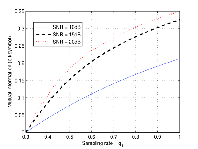
Fig. 7 shows the secrecy rate as a function of q1subscript𝑞1q_{1} and the SNR for p=0.2𝑝0.2p=0.2 and q2=0.3subscript𝑞20.3q_{2}=0.3. It can be seen that when q1=q2subscript𝑞1subscript𝑞2q_{1}=q_{2} the secrecy rate vanishes, as one should expect. Also, for any q1>0.3subscript𝑞10.3q_{1}>0.3, increasing the SNR resulting in an increasing of the secrecy rate, and similarly stronger legitimate receivers can achieve higher secrecy rate.
Refer to caption

Figure 7: Secrecy rate when the sparsity pattern is controlled, as a function of q1subscript𝑞1q_{1} and the SNR, for p=0.2𝑝0.2p=0.2 and q2=0.3subscript𝑞20.3q_{2}=0.3.

V-B Unavailable sparsity pattern

In this subsection, we consider the case where the sparsity pattern is known to nobody, and the vector 𝑼𝑼U is treated as the information to be transmitted over the channel. As before, since we deal with degraded channels, our setting is just a special case of [25], and the secrecy rate is now given by

limn1n[I(𝒀1;𝑼|𝑨1,𝑯1)I(𝒀2;𝑼|𝑨2,𝑯2)]subscript𝑛1𝑛delimited-[]𝐼subscript𝒀1conditional𝑼subscript𝑨1subscript𝑯1𝐼subscript𝒀2conditional𝑼subscript𝑨2subscript𝑯2\displaystyle\lim_{n\to\infty}\frac{1}{n}\left[I\left(\mbox{\boldmath$Y$}_{1};\mbox{\boldmath$U$}|\mbox{\boldmath$A$}_{1},\mbox{\boldmath$H$}_{1}\right)-I\left(\mbox{\boldmath$Y$}_{2};\mbox{\boldmath$U$}|\mbox{\boldmath$A$}_{2},\mbox{\boldmath$H$}_{2}\right)\right] (67)

Thus, we have the following result.

Theorem 10 (unavailable sparsity pattern)

Assume that 𝑺𝑺S is known to nobody. Then, an achievable secrecy rate is given by

1,L2,E2(p)subscript1𝐿subscript2𝐸subscript2𝑝\displaystyle{\cal I}_{1,L}-{\cal I}_{2,E}-{\cal H}_{2}\left(p\right) (68)
Proof 7

Using (67), we note that

I(𝒀1;𝑼|𝑨1,𝑯1)I(𝒀2;𝑼|𝑨2,𝑯2)𝐼subscript𝒀1conditional𝑼subscript𝑨1subscript𝑯1𝐼subscript𝒀2conditional𝑼subscript𝑨2subscript𝑯2\displaystyle I\left(\mbox{\boldmath$Y$}_{1};\mbox{\boldmath$U$}|\mbox{\boldmath$A$}_{1},\mbox{\boldmath$H$}_{1}\right)-I\left(\mbox{\boldmath$Y$}_{2};\mbox{\boldmath$U$}|\mbox{\boldmath$A$}_{2},\mbox{\boldmath$H$}_{2}\right) =(a)I(𝑿;𝒀1|𝑨1,𝑯1)I(𝑺;𝒀1|𝑼,𝑨1,𝑯1)superscript𝑎absent𝐼𝑿conditionalsubscript𝒀1subscript𝑨1subscript𝑯1𝐼𝑺conditionalsubscript𝒀1𝑼subscript𝑨1subscript𝑯1\displaystyle\stackrel{{\scriptstyle(a)}}{{=}}I\left(\mbox{\boldmath$X$};\mbox{\boldmath$Y$}_{1}|\mbox{\boldmath$A$}_{1},\mbox{\boldmath$H$}_{1}\right)-I\left(\mbox{\boldmath$S$};\mbox{\boldmath$Y$}_{1}|\mbox{\boldmath$U$},\mbox{\boldmath$A$}_{1},\mbox{\boldmath$H$}_{1}\right)
I(𝑿;𝒀2|𝑨2,𝑯2)+I(𝑺;𝒀2|𝑼,𝑨2,𝑯2)𝐼𝑿conditionalsubscript𝒀2subscript𝑨2subscript𝑯2𝐼𝑺conditionalsubscript𝒀2𝑼subscript𝑨2subscript𝑯2\displaystyle\ \ \ -I\left(\mbox{\boldmath$X$};\mbox{\boldmath$Y$}_{2}|\mbox{\boldmath$A$}_{2},\mbox{\boldmath$H$}_{2}\right)+I\left(\mbox{\boldmath$S$};\mbox{\boldmath$Y$}_{2}|\mbox{\boldmath$U$},\mbox{\boldmath$A$}_{2},\mbox{\boldmath$H$}_{2}\right) (69)
(b)I(𝑿;𝒀1|𝑨1,𝑯1)H(𝑺)superscript𝑏absent𝐼𝑿conditionalsubscript𝒀1subscript𝑨1subscript𝑯1𝐻𝑺\displaystyle\stackrel{{\scriptstyle(b)}}{{\geq}}I\left(\mbox{\boldmath$X$};\mbox{\boldmath$Y$}_{1}|\mbox{\boldmath$A$}_{1},\mbox{\boldmath$H$}_{1}\right)-H\left(\mbox{\boldmath$S$}\right)
I(𝑿;𝒀2|𝑨2,𝑯2)+I(𝑺;𝒀2|𝑨2,𝑯2)𝐼𝑿conditionalsubscript𝒀2subscript𝑨2subscript𝑯2𝐼𝑺conditionalsubscript𝒀2subscript𝑨2subscript𝑯2\displaystyle\ \ \ -I\left(\mbox{\boldmath$X$};\mbox{\boldmath$Y$}_{2}|\mbox{\boldmath$A$}_{2},\mbox{\boldmath$H$}_{2}\right)+I\left(\mbox{\boldmath$S$};\mbox{\boldmath$Y$}_{2}|\mbox{\boldmath$A$}_{2},\mbox{\boldmath$H$}_{2}\right) (70)
(c)I(𝑿;𝒀1|𝑨1,𝑯1)H(𝑺)I(𝑼;𝒀2|𝑨2,𝑯2,𝑺)superscript𝑐absent𝐼𝑿conditionalsubscript𝒀1subscript𝑨1subscript𝑯1𝐻𝑺𝐼𝑼conditionalsubscript𝒀2subscript𝑨2subscript𝑯2𝑺\displaystyle\stackrel{{\scriptstyle(c)}}{{\geq}}I\left(\mbox{\boldmath$X$};\mbox{\boldmath$Y$}_{1}|\mbox{\boldmath$A$}_{1},\mbox{\boldmath$H$}_{1}\right)-H\left(\mbox{\boldmath$S$}\right)-I\left(\mbox{\boldmath$U$};\mbox{\boldmath$Y$}_{2}|\mbox{\boldmath$A$}_{2},\mbox{\boldmath$H$}_{2},\mbox{\boldmath$S$}\right) (71)

where (a)𝑎(a) follows from the chain rule of the mutual information, (b)𝑏(b) follows from the fact that I(𝑺;𝒀2|𝑼,𝑨2,𝑯2)I(𝑺;𝒀2|𝑨2,𝑯2)𝐼𝑺conditionalsubscript𝒀2𝑼subscript𝑨2subscript𝑯2𝐼𝑺conditionalsubscript𝒀2subscript𝑨2subscript𝑯2I\left(\mbox{\boldmath$S$};\mbox{\boldmath$Y$}_{2}|\mbox{\boldmath$U$},\mbox{\boldmath$A$}_{2},\mbox{\boldmath$H$}_{2}\right)\geq I\left(\mbox{\boldmath$S$};\mbox{\boldmath$Y$}_{2}|\mbox{\boldmath$A$}_{2},\mbox{\boldmath$H$}_{2}\right), which in turn is due to

I(𝑺;𝒀2|𝑨2,𝑯2)𝐼𝑺conditionalsubscript𝒀2subscript𝑨2subscript𝑯2\displaystyle I\left(\mbox{\boldmath$S$};\mbox{\boldmath$Y$}_{2}|\mbox{\boldmath$A$}_{2},\mbox{\boldmath$H$}_{2}\right) I(𝑺;𝒀2,𝑼|𝑨2,𝑯2)absent𝐼𝑺subscript𝒀2conditional𝑼subscript𝑨2subscript𝑯2\displaystyle\leq I\left(\mbox{\boldmath$S$};\mbox{\boldmath$Y$}_{2},\mbox{\boldmath$U$}|\mbox{\boldmath$A$}_{2},\mbox{\boldmath$H$}_{2}\right) (72)
=I(𝑺;𝑼|𝑨2,𝑯2)+I(𝑺;𝒀2|𝑼𝑨2,𝑯2)absent𝐼𝑺conditional𝑼subscript𝑨2subscript𝑯2𝐼𝑺conditionalsubscript𝒀2subscript𝑼𝑨2subscript𝑯2\displaystyle=I\left(\mbox{\boldmath$S$};\mbox{\boldmath$U$}|\mbox{\boldmath$A$}_{2},\mbox{\boldmath$H$}_{2}\right)+I\left(\mbox{\boldmath$S$};\mbox{\boldmath$Y$}_{2}|\mbox{\boldmath$U$}\mbox{\boldmath$A$}_{2},\mbox{\boldmath$H$}_{2}\right) (73)
=I(𝑺;𝒀2|𝑼,𝑨2,𝑯2)absent𝐼𝑺conditionalsubscript𝒀2𝑼subscript𝑨2subscript𝑯2\displaystyle=I\left(\mbox{\boldmath$S$};\mbox{\boldmath$Y$}_{2}|\mbox{\boldmath$U$},\mbox{\boldmath$A$}_{2},\mbox{\boldmath$H$}_{2}\right) (74)

where the first passage is due to the data processing inequality. Finally, (b)𝑏(b) follows from (59). Therefore, (68) readily follows from (71).

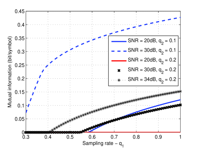
Fig. 8 shows the secrecy rate as a function of q1subscript𝑞1q_{1} for p=0.2𝑝0.2p=0.2, various values of the SNR, and q2=0.1subscript𝑞20.1q_{2}=0.1 and q2=0.2subscript𝑞20.2q_{2}=0.2. The results illustrate, again, the importance of controlling the sparsity pattern.
Refer to caption

Figure 8: Secrecy rate when the sparsity pattern is unavailable, as a function of q1subscript𝑞1q_{1} and the SNR, for p=0.2𝑝0.2p=0.2 and q2=0.3subscript𝑞20.3q_{2}=0.3.

V-C Uncontrolled sparsity pattern

Finally, we consider the case in which 𝑺𝑺S is non-causally available to the transmitter, but cannot be controlled, that is, 𝑺𝑺S plays the role of a state as in Subsection IV-B. The problem of secrecy capacity here, is not fully solved, but an insightful achievable region was found in [26]. This achievable rate is given by

limn1n[I(𝑽;𝒀1|𝑨1,𝑯1)max{I(𝑽;𝑺),I(𝑽;𝒀2|𝑨2,𝑯2)}]subscript𝑛1𝑛delimited-[]𝐼𝑽conditionalsubscript𝒀1subscript𝑨1subscript𝑯1𝐼𝑽𝑺𝐼𝑽conditionalsubscript𝒀2subscript𝑨2subscript𝑯2\displaystyle\lim_{n\to\infty}\frac{1}{n}\left[I\left(\mbox{\boldmath$V$};\mbox{\boldmath$Y$}_{1}|\mbox{\boldmath$A$}_{1},\mbox{\boldmath$H$}_{1}\right)-\max\left\{I\left(\mbox{\boldmath$V$};\mbox{\boldmath$S$}\right),I\left(\mbox{\boldmath$V$};\mbox{\boldmath$Y$}_{2}|\mbox{\boldmath$A$}_{2},\mbox{\boldmath$H$}_{2}\right)\right\}\right] (75)

where 𝑽(𝑼,𝑺)(𝒀1,𝒀2)𝑽𝑼𝑺subscript𝒀1subscript𝒀2\mbox{\boldmath$V$}-\left(\mbox{\boldmath$U$},\mbox{\boldmath$S$}\right)-\left(\mbox{\boldmath$Y$}_{1},\mbox{\boldmath$Y$}_{2}\right). Note that, as before, 𝒀2subscript𝒀2\mbox{\boldmath$Y$}_{2} can be represented as a degraded version of 𝒀1subscript𝒀1\mbox{\boldmath$Y$}_{1}. Evidently, this achievable rate is again composed of 1subscript1{\cal I}_{1} terms, as well as I(𝑽;𝑺)𝐼𝑽𝑺I\left(\mbox{\boldmath$V$};\mbox{\boldmath$S$}\right). Taking 𝑽=𝑺𝑼𝑽𝑺𝑼\mbox{\boldmath$V$}=\mbox{\boldmath$S$}\mbox{\boldmath$U$}, we obtain the following result.

Theorem 11 (uncontrolled sparsity pattern)

Assume that 𝑺𝑺S is a non-causal state information, that is unavailable a-priori to both the legitimate user and the eavesdropper. Then, the achievable secrecy rate is given by

R=1,Lmax{2(p),1,E}.𝑅subscript1𝐿subscript2𝑝subscript1𝐸\displaystyle R={\cal I}_{1,L}-\max\left\{{\cal H}_{2}\left(p\right),{\cal I}_{1,E}\right\}. (76)

Theorems 8 and 11 demonstrate some gain that results from the ability to control the sparsity pattern control the sparsity pattern 𝑺𝑺S. Indeed, it can be seen that for high SNR there is no difference between the two achievable secrecy rates. However, below some SNR level, when the sparsity pattern cannot be controlled, the binary entropy 2(p)subscript2𝑝{\cal H}_{2}\left(p\right) dominates 1,Esubscript1𝐸{\cal I}_{1,E}, and the resulting secrecy rate is smaller than the secrecy rate in case of controlled sparsity pattern.

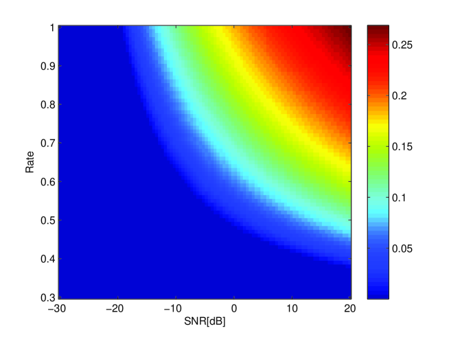
Fig. 9 shows the achievable rate as a function of q1subscript𝑞1q_{1} and the SNR, for p=0.2𝑝0.2p=0.2 and q2=0.3subscript𝑞20.3q_{2}=0.3. It can be seen that the result is similar to Fig. 6, that is

1,Lmax{2(p),1,E}=1,L2(p).subscript1𝐿subscript2𝑝subscript1𝐸subscript1𝐿subscript2𝑝\displaystyle{\cal I}_{1,L}-\max\left\{{\cal H}_{2}\left(p\right),{\cal I}_{1,E}\right\}={\cal I}_{1,L}-{\cal H}_{2}\left(p\right). (77)

Accordingly, this means that under the above specific choice of p𝑝p and q2subscript𝑞2q_{2}, the loss in the secrecy rate is attributed more to the fact that the sparsity pattern cannot be controlled, than due to the presence of a wiretapper.
Refer to caption

Figure 9: Secrecy rate in case of an uncontrolled sparsity pattern, as a function of q1subscript𝑞1q_{1} and the SNR, for p=0.2𝑝0.2p=0.2 and q2=0.3subscript𝑞20.3q_{2}=0.3.

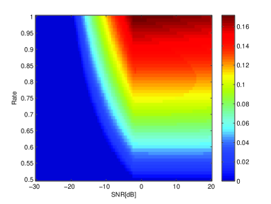
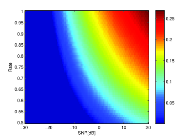
In order to illustrate the loss due to the wiretapper, we consider the following example. Figures 10a and 10b show, respectively, the achievable rate and 1,L2(p)subscript1𝐿subscript2𝑝{\cal I}_{1,L}-{\cal H}_{2}\left(p\right), as a function of q1subscript𝑞1q_{1} and the SNR, for p=0.2𝑝0.2p=0.2 and q2=0.5subscript𝑞20.5q_{2}=0.5. In this case the eavesdropper has a strong processor, so it can process more measurements compared to the previous example. Accordingly, it is evident that in this case the wiretapper plays a role, and the loss in the secrecy rate is now more significant.
Refer to caption
(a)
Refer to caption
(b)
Figure 10: (a) Secrecy rate and (b) 1,L2(p)subscript1𝐿subscript2𝑝{\cal I}_{1,L}-{\cal H}_{2}\left(p\right) in case of an uncontrolled sparsity pattern as a function of q1subscript𝑞1q_{1} and the SNR, for p=0.2𝑝0.2p=0.2 and q2=0.5subscript𝑞20.5q_{2}=0.5.

VI The Multiple Access Channel

In this section, we consider the symmetric333The symmetry is in the sense that all the users transmit at equal power levels. MAC settings [27], in which several senders send information to a common receiver. In our case, we have the following setting: The sequence {Ui}subscript𝑈𝑖\left\{U_{i}\right\} are now the signals corresponding to different non-cooperative remote users, and the constraint is that on the average, one cannot employ more than pn𝑝𝑛pn transmit antennas. The pattern sequence is assumed to be i.i.d. Here, the i𝑖ith user can control the signal Uisubscript𝑈𝑖U_{i}, as well as Sisubscript𝑆𝑖S_{i} (adhering, of course, to the rule that (Si=1)=psubscript𝑆𝑖1𝑝\mathbb{P}\left(S_{i}=1\right)=p). We have the following result.

Theorem 12 (MAC)

Consider the MAC under the aforementioned assumptions, and let (R1,,Rn)subscript𝑅1subscript𝑅𝑛\left(R_{1},\ldots,R_{n}\right) denote the rates of the n𝑛n users. Then,

α(1α)11,αsubscript𝛼superscript1𝛼1subscript1𝛼\displaystyle{\cal R}_{\alpha}\leq\left(1-\alpha\right)^{-1}{\cal I}_{1,\alpha} (78)

where αsubscript𝛼{\cal R}_{\alpha} is the sum-rates of n(1α)𝑛1𝛼n\left(1-\alpha\right) users (no matter which ones, due to symmetry), where 0α<10𝛼10\leq\alpha<1, and 1,αsubscript1𝛼{\cal I}_{1,\alpha} equals to 1subscript1{\cal I}_{1} but with p𝑝p replaced by (1α)p1𝛼𝑝\left(1-\alpha\right)p. Particularity, the sum-rates (corresponding to α=0𝛼0\alpha=0) is given by 1subscript1{\cal I}_{1}.

Proof 8

The case of α=0𝛼0\alpha=0 follows directly from the MAC capacity region [27]. For the second part, we wish to find the achievable rate of n(1α)𝑛1𝛼n\left(1-\alpha\right) users, namely, in the MAC capacity region we condition on the signals produced by the other nα𝑛𝛼n\alpha users, and the achievable is given by

I(𝑿(1α);𝒀|𝑿α,𝑨,𝑯)𝐼subscript𝑿1𝛼conditional𝒀subscript𝑿𝛼𝑨𝑯\displaystyle I\left(\mbox{\boldmath$X$}_{\left(1-\alpha\right)};\mbox{\boldmath$Y$}|\mbox{\boldmath$X$}_{\alpha},\mbox{\boldmath$A$},\mbox{\boldmath$H$}\right) (79)

where 𝑿αsubscript𝑿𝛼\mbox{\boldmath$X$}_{\alpha} (and similarly for 𝑿(1α)subscript𝑿1𝛼\mbox{\boldmath$X$}_{\left(1-\alpha\right)}) correspond to the nα𝑛𝛼n\alpha users. This can be thought as

𝒀𝒀Y =𝑨𝑯𝑿+𝑾absent𝑨𝑯𝑿𝑾\displaystyle=\mbox{\boldmath$A$}\mbox{\boldmath$H$}\mbox{\boldmath$X$}+\mbox{\boldmath$W$} (80)
=𝑨𝑯𝑿(1α)+𝑨𝑯𝑿α+𝑾,absentsubscript𝑨𝑯𝑿1𝛼subscript𝑨𝑯𝑿𝛼𝑾\displaystyle=\mbox{\boldmath$A$}\mbox{\boldmath$H$}\mbox{\boldmath$X$}_{\left(1-\alpha\right)}+\mbox{\boldmath$A$}\mbox{\boldmath$H$}\mbox{\boldmath$X$}_{\alpha}+\mbox{\boldmath$W$}, (81)

and thus (79) is equivalent as to examine 1subscript1{\cal I}_{1} but with p(1α)pmaps-to𝑝1𝛼𝑝p\mapsto\left(1-\alpha\right)p. Finally, due to the fact that 1subscript1{\cal I}_{1} is normalized by n𝑛n, we need to re-normalize the result by multiplying it by (1α)1superscript1𝛼1(1-\alpha)^{-1}.

VII Conclusions

In this paper, we examine the problem of sparse sampling of coded signals under several basic channel coding problems. In the first part, we present closed-form single-letter expressions for the input-output mutual information rates, assuming a compressed Gaussian linear channel model. These results are based on rigorous analytical derivations which agree with previously derived results of the replica method. In the second part, we present achievable rates in several channel coding problems, in the wiretap channel model, and in the multiple access channel (MAC). Specifically, for channel coding problem, we consider three cases that differ in the available knowledge of the transmitter and the receiver about the source, and particularity, regarding the sparsity pattern. The results quantify, for example, how important is it to be able to control the sparsity pattern. Also, we show that when this pattern can be controlled by the transmitted, then, a memoryless source maximizes the mutual information rate, given some sparsity average constraint. Then, we consider the wiretap channel model for which several cases were studied. The problems considered are timely and motivated by processing limitations, where the legitimate receiver has stronger processors, and hence can process more outputs/measurements, going via different jamming patterns, as well as cloud processing. Here, the results demonstrate, for example, our inherent limits in achieving some degree of secrecy as a function of the sampling rates of the legitimate user and the eavesdropper. Finally, in a fashion similar to the previous discussion, in case that the sparsity pattern can be controlled by the transmitter, we show that the secrecy rate cannot be increased by using sparsity patterns that are not memoryless.

Appendix A Proof Outline of Theorem 1

In this appendix, we give a proof outline of Theorem 1. It should be emphasized that Theorem 1 is a special case of the problem considered in [1], and here we emphasize the required modifications. The analysis consists of three main steps, which will be presented in the sequel, along with specific pointers to the proof in [1].

The first step in the analysis is to find a generic expression of the mutual information for fixed k,n𝑘𝑛k,n. This is done by using a relationship between the mutual information and some partition function [28]. To this end, we define the following function,

Z(𝒚,𝑯,𝑨)=nμ(d𝒙)exp[𝒚𝑨𝑯𝒙2/2].superscript𝑍𝒚𝑯𝑨subscriptsuperscript𝑛𝜇d𝒙superscriptnorm𝒚𝑨𝑯𝒙22\displaystyle Z\left(\mbox{\boldmath$y$},\mbox{\boldmath$H$},\mbox{\boldmath$A$}\right)\stackrel{{\scriptstyle\triangle}}{{=}}\int_{\mathbb{R}^{n}}\mu\left(\mathrm{d}\mbox{\boldmath$x$}\right)\exp\left[-\left\|\mbox{\boldmath$y$}-\mbox{\boldmath$A$}\mbox{\boldmath$H$}\mbox{\boldmath$x$}\right\|^{2}/2\right]. (A.1)

According to our source model assumptions, the input distribution is given by

μ(𝒙)=𝒔{0,1}n(𝒔)i:si=0δ(xi)i:si=112πσ2e12σ2xi2.𝜇𝒙subscript𝒔superscript01𝑛𝒔subscriptproduct:𝑖subscript𝑠𝑖0𝛿subscript𝑥𝑖subscriptproduct:𝑖subscript𝑠𝑖112𝜋superscript𝜎2superscript𝑒12superscript𝜎2superscriptsubscript𝑥𝑖2\displaystyle\mu\left(\mbox{\boldmath$x$}\right)=\sum_{\mbox{\footnotesize\boldmath$s$}\in\left\{0,1\right\}^{n}}\mathbb{P}\left(\mbox{\boldmath$s$}\right)\prod_{i:\;s_{i}=0}\delta\left(x_{i}\right)\prod_{i:\;s_{i}=1}\frac{1}{\sqrt{2\pi\sigma^{2}}}e^{-\frac{1}{2\sigma^{2}}x_{i}^{2}}. (A.2)

Now,

I(𝒀;𝑿|𝑨,𝑯)𝐼𝒀conditional𝑿𝑨𝑯\displaystyle I\left(\mbox{\boldmath$Y$};\mbox{\boldmath$X$}|\mbox{\boldmath$A$},\mbox{\boldmath$H$}\right) =𝔼{logexp(𝒀𝑨𝑯𝑿2/2)Z(𝒚,𝑯,𝑨)}absent𝔼superscriptnorm𝒀𝑨𝑯𝑿22𝑍𝒚𝑯𝑨\displaystyle=\mathbb{E}\left\{\log\frac{\exp\left(-\left\|\mbox{\boldmath$Y$}-\mbox{\boldmath$A$}\mbox{\boldmath$H$}\mbox{\boldmath$X$}\right\|^{2}/2\right)}{Z\left(\mbox{\boldmath$y$},\mbox{\boldmath$H$},\mbox{\boldmath$A$}\right)}\right\} (A.3)
=12𝔼{𝒀𝑨𝑯𝑿2}𝔼{logZ(𝒚,𝑯,𝑨)}absent12𝔼superscriptnorm𝒀𝑨𝑯𝑿2𝔼𝑍𝒚𝑯𝑨\displaystyle=-\frac{1}{2}\mathbb{E}\left\{\left\|\mbox{\boldmath$Y$}-\mbox{\boldmath$A$}\mbox{\boldmath$H$}\mbox{\boldmath$X$}\right\|^{2}\right\}-\mathbb{E}\left\{\log Z\left(\mbox{\boldmath$y$},\mbox{\boldmath$H$},\mbox{\boldmath$A$}\right)\right\} (A.4)
=n2𝔼{logZ(𝒀,𝑯,𝑨)}.absent𝑛2𝔼𝑍𝒀𝑯𝑨\displaystyle=-\frac{n}{2}-\mathbb{E}\left\{\log Z\left(\mbox{\boldmath$Y$},\mbox{\boldmath$H$},\mbox{\boldmath$A$}\right)\right\}. (A.5)

Next, as shown in444In the notation of [1], 𝑯𝑯H and 𝑯𝒔subscript𝑯𝒔\mbox{\boldmath$H$}_{\mbox{\footnotesize\boldmath$s$}} correspond to 𝑨𝑨A𝑯𝑯H and 𝑨𝑯𝒔subscript𝑨𝑯𝒔\mbox{\boldmath$A$}\mbox{\boldmath$H$}_{\mbox{\footnotesize\boldmath$s$}} in our notations. [1, Eqs. (57)-(64)]

Z(𝒚,𝑨,𝑯)𝑍𝒚𝑨𝑯\displaystyle Z\left(\mbox{\boldmath$y$},\mbox{\boldmath$A$},\mbox{\boldmath$H$}\right) =exp(12𝒚2)𝒔{0,1}n(𝒔)𝒢(𝒚,𝑨,𝑯𝒔)absent12superscriptnorm𝒚2subscript𝒔superscript01𝑛𝒔𝒢𝒚𝑨subscript𝑯𝒔\displaystyle=\exp\left(-\frac{1}{2}\left\|\mbox{\boldmath$y$}\right\|^{2}\right)\cdot\sum_{\mbox{\boldmath$s$}\in\left\{0,1\right\}^{n}}\mathbb{P}\left(\mbox{\boldmath$s$}\right){\cal G}\left(\mbox{\boldmath$y$},\mbox{\boldmath$A$},\mbox{\boldmath$H$}_{\mbox{\footnotesize\boldmath$s$}}\right) (A.6)

where

𝒢(𝒚,𝑨,𝑯𝒔)=exp{12𝒚T𝑨𝑯𝒔𝓗𝒔𝑯𝒔T𝑨T𝒚}det(σ2𝑯𝒔T𝑨T𝑨𝑯𝒔+𝑰𝒔),superscript𝒢𝒚𝑨subscript𝑯𝒔12superscript𝒚𝑇subscript𝑨𝑯𝒔superscriptsubscript𝓗𝒔𝑯𝒔𝑇superscript𝑨𝑇𝒚superscript𝜎2superscriptsubscript𝑯𝒔𝑇superscript𝑨𝑇subscript𝑨𝑯𝒔subscript𝑰𝒔\displaystyle{\cal G}\left(\mbox{\boldmath$y$},\mbox{\boldmath$A$},\mbox{\boldmath$H$}_{\mbox{\footnotesize\boldmath$s$}}\right)\stackrel{{\scriptstyle\triangle}}{{=}}\frac{\exp\left\{\frac{1}{2}\mbox{\boldmath$y$}^{T}\mbox{\boldmath$A$}\mbox{\boldmath$H$}_{\mbox{\footnotesize\boldmath$s$}}\mbox{\boldmath${\cal H}^{\mbox{\footnotesize\boldmath$s$}}$}\mbox{\boldmath$H$}_{\mbox{\footnotesize\boldmath$s$}}^{T}\mbox{\boldmath$A$}^{T}\mbox{\boldmath$y$}\right\}}{\sqrt{\det\left(\sigma^{2}\mbox{\boldmath$H$}_{\mbox{\footnotesize\boldmath$s$}}^{T}\mbox{\boldmath$A$}^{T}\mbox{\boldmath$A$}\mbox{\boldmath$H$}_{\mbox{\footnotesize\boldmath$s$}}+\mbox{\boldmath$I$}_{\mbox{\footnotesize\boldmath$s$}}\right)}}, (A.7)

where 𝑯𝒔subscript𝑯𝒔\mbox{\boldmath$H$}_{\mbox{\footnotesize\boldmath$s$}} denotes the restriction of 𝑯𝑯H on the support 𝒮={i:Si0}𝒮conditional-set𝑖subscript𝑆𝑖0{\cal S}=\left\{i\in\mathbb{N}:S_{i}\neq 0\right\}, and 𝓗𝒔=(𝑯𝒔T𝑨T𝑨𝑯𝒔+1σ2𝑰𝒔)1superscriptsuperscript𝓗𝒔superscriptsuperscriptsubscript𝑯𝒔𝑇superscript𝑨𝑇subscript𝑨𝑯𝒔1superscript𝜎2subscript𝑰𝒔1\mbox{\boldmath${\cal H}^{\mbox{\footnotesize\boldmath$s$}}$}\stackrel{{\scriptstyle\triangle}}{{=}}\left(\mbox{\boldmath$H$}_{\mbox{\footnotesize\boldmath$s$}}^{T}\mbox{\boldmath$A$}^{T}\mbox{\boldmath$A$}\mbox{\boldmath$H$}_{\mbox{\footnotesize\boldmath$s$}}+\frac{1}{\sigma^{2}}\mbox{\boldmath$I$}_{\mbox{\footnotesize\boldmath$s$}}\right)^{-1}. Thus,

I(𝒀;𝑿|𝑨,𝑯)n𝐼𝒀conditional𝑿𝑨𝑯𝑛\displaystyle\frac{I\left(\mbox{\boldmath$Y$};\mbox{\boldmath$X$}|\mbox{\boldmath$A$},\mbox{\boldmath$H$}\right)}{n} =12+12[maσ2q+1]1n𝔼{log𝒔{0,1}n(𝒔)𝒢(𝒀,𝑨,𝑯𝒔)}absent1212delimited-[]subscript𝑚𝑎superscript𝜎2𝑞11𝑛𝔼subscript𝒔superscript01𝑛𝒔𝒢𝒀𝑨subscript𝑯𝒔\displaystyle=-\frac{1}{2}+\frac{1}{2}\left[m_{a}\sigma^{2}q+1\right]-\frac{1}{n}\mathbb{E}\left\{\log\sum_{\mbox{\boldmath$s$}\in\left\{0,1\right\}^{n}}\mathbb{P}\left(\mbox{\boldmath$s$}\right){\cal G}\left(\mbox{\boldmath$Y$},\mbox{\boldmath$A$},\mbox{\boldmath$H$}_{\mbox{\footnotesize\boldmath$s$}}\right)\right\}
=12σ2maq1n𝔼{log𝒔{0,1}n(𝒔)𝒢(𝒀,𝑨,𝑯𝒔)},absent12superscript𝜎2subscript𝑚𝑎𝑞1𝑛𝔼subscript𝒔superscript01𝑛𝒔𝒢𝒀𝑨subscript𝑯𝒔\displaystyle=\frac{1}{2}\sigma^{2}m_{a}q-\frac{1}{n}\mathbb{E}\left\{\log\sum_{\mbox{\boldmath$s$}\in\left\{0,1\right\}^{n}}\mathbb{P}\left(\mbox{\boldmath$s$}\right){\cal G}\left(\mbox{\boldmath$Y$},\mbox{\boldmath$A$},\mbox{\boldmath$H$}_{\mbox{\footnotesize\boldmath$s$}}\right)\right\}, (A.8)

and therefore, in view of (A.8), we wish to calculate the limit

limn1n𝔼{log𝒵n(𝒀,𝑨,𝑯)}=limn1n𝔼{log𝒔{0,1}n(𝒔)𝒢(𝒚,𝑨,𝑯𝒔)}.superscriptsubscript𝑛1𝑛𝔼subscript𝒵𝑛𝒀𝑨𝑯subscript𝑛1𝑛𝔼subscript𝒔superscript01𝑛𝒔𝒢𝒚𝑨subscript𝑯𝒔\displaystyle\lim_{n\to\infty}\frac{1}{n}\mathbb{E}\left\{\log\mathscr{Z}_{n}\left(\mbox{\boldmath$Y$},\mbox{\boldmath$A$},\mbox{\boldmath$H$}\right)\right\}\stackrel{{\scriptstyle\triangle}}{{=}}\lim_{n\to\infty}\frac{1}{n}\mathbb{E}\left\{\log\sum_{\mbox{\boldmath$s$}\in\left\{0,1\right\}^{n}}\mathbb{P}\left(\mbox{\boldmath$s$}\right){\cal G}\left(\mbox{\boldmath$y$},\mbox{\boldmath$A$},\mbox{\boldmath$H$}_{\mbox{\footnotesize\boldmath$s$}}\right)\right\}. (A.9)

This concludes the first step. Now, it can be seen from (A.7) that (A.9) contains terms that are recognized as an extended version of the Stieltjes and Shannon transforms [29] of the matrix 𝑯𝒔T𝑨T𝑨𝑯𝒔superscriptsubscript𝑯𝒔𝑇superscript𝑨𝑇subscript𝑨𝑯𝒔\mbox{\boldmath$H$}_{\mbox{\footnotesize\boldmath$s$}}^{T}\mbox{\boldmath$A$}^{T}\mbox{\boldmath$A$}\mbox{\boldmath$H$}_{\mbox{\footnotesize\boldmath$s$}}. In the field of random matrix theory, there is a great interest in exploring the asymptotic behavior, and in particular finding the deterministic equivalent of such transforms (see, for example, [12, 13]). Evidently, under some conditions, it is well-known that these transforms asymptotically converge for a fairly wide family of matrices.

Following the last observation, in the second step, we show that these functions converge, with probability tending to one, as n𝑛n\to\infty, to some random functions that are much easier to work with. Accordingly, the following lemma is essentially the core of our analysis; it provides approximations (which are asymptotically exact in the almost sure (a.s.) sense) of 𝒢𝒢{\cal G} and (A.9). For simplicity of notations, we let ms=n1i=1nsisuperscriptsubscript𝑚𝑠superscript𝑛1superscriptsubscript𝑖1𝑛subscript𝑠𝑖m_{s}\stackrel{{\scriptstyle\triangle}}{{=}}n^{-1}\sum_{i=1}^{n}s_{i}, and recall the auxiliary variables defined in (12)-(17). The following lemma is proved in [1, Appendix B, C].

Lemma 1 (asymptotic equivalence)

Under the assumptions and definition presented earlier, the following relations hold in the almost sure (a.s.) sense:

limn1nlndet(σ2𝑯𝒔T𝑨T𝑨𝑯𝒔+𝑰𝒔)=msI¯(ms),subscript𝑛1𝑛superscript𝜎2superscriptsubscript𝑯𝒔𝑇superscript𝑨𝑇subscript𝑨𝑯𝒔subscript𝑰𝒔subscript𝑚𝑠¯𝐼subscript𝑚𝑠\displaystyle\lim_{n\to\infty}\frac{1}{n}\ln\det\left(\sigma^{2}\mbox{\boldmath$H$}_{\mbox{\footnotesize\boldmath$s$}}^{T}\mbox{\boldmath$A$}^{T}\mbox{\boldmath$A$}\mbox{\boldmath$H$}_{\mbox{\footnotesize\boldmath$s$}}+\mbox{\boldmath$I$}_{\mbox{\footnotesize\boldmath$s$}}\right)=m_{s}\bar{I}\left(m_{s}\right), (A.10)

and

limn1n[𝒚T𝑨𝑯𝒔𝓗𝒔𝑯𝒔T𝑨T𝒚fn]=0,subscript𝑛1𝑛delimited-[]superscript𝒚𝑇subscript𝑨𝑯𝒔superscriptsubscript𝓗𝒔𝑯𝒔𝑇superscript𝑨𝑇𝒚subscript𝑓𝑛0\displaystyle\lim_{n\to\infty}\frac{1}{n}\left[\mbox{\boldmath$y$}^{T}\mbox{\boldmath$A$}\mbox{\boldmath$H$}_{\mbox{\footnotesize\boldmath$s$}}\mbox{\boldmath${\cal H}^{\mbox{\footnotesize\boldmath$s$}}$}\mbox{\boldmath$H$}_{\mbox{\footnotesize\boldmath$s$}}^{T}\mbox{\boldmath$A$}^{T}\mbox{\boldmath$y$}-f_{n}\right]=0, (A.11)

where

fn=2V(ms)𝒚2n+2L(ms)𝑯𝒔T𝑨T𝒚2n.superscriptsubscript𝑓𝑛2𝑉subscript𝑚𝑠superscriptnorm𝒚2𝑛2𝐿subscript𝑚𝑠superscriptnormsuperscriptsubscript𝑯𝒔𝑇superscript𝑨𝑇𝒚2𝑛\displaystyle f_{n}\stackrel{{\scriptstyle\triangle}}{{=}}2\cdot V\left(m_{s}\right)\frac{\left\|\mbox{\boldmath$y$}\right\|^{2}}{n}+2\cdot L\left(m_{s}\right)\frac{\left\|\mbox{\boldmath$H$}_{\mbox{\footnotesize\boldmath$s$}}^{T}\mbox{\boldmath$A$}^{T}\mbox{\boldmath$y$}\right\|^{2}}{n}. (A.12)

Finally, for large n𝑛n and k𝑘k, and for (𝒚,𝑨,𝑯)𝒚𝑨𝑯\left(\mbox{\boldmath$y$},\mbox{\boldmath$A$},\mbox{\boldmath$H$}\right)-typical sequences, the function 𝒵n(𝒚,𝑨,𝑯)subscript𝒵𝑛𝒚𝑨𝑯\mathscr{Z}_{n}\left(\mbox{\boldmath$y$},\mbox{\boldmath$A$},\mbox{\boldmath$H$}\right) is lower and upper bounded as follows

𝒵(𝒚,𝑨,𝑯)𝒵n(𝒚,𝑨,𝑯)𝒵+(𝒚,𝑨,𝑯),subscript𝒵𝒚𝑨𝑯subscript𝒵𝑛𝒚𝑨𝑯subscript𝒵𝒚𝑨𝑯\displaystyle\mathscr{Z}_{-}\left(\mbox{\boldmath$y$},\mbox{\boldmath$A$},\mbox{\boldmath$H$}\right)\leq\mathscr{Z}_{n}\left(\mbox{\boldmath$y$},\mbox{\boldmath$A$},\mbox{\boldmath$H$}\right)\leq\mathscr{Z}_{+}\left(\mbox{\boldmath$y$},\mbox{\boldmath$A$},\mbox{\boldmath$H$}\right), (A.13)

where

𝒵±(𝒚,𝑨,𝑯)=Cn𝒔{0,1}nexp{n(t~(ms)+L(ms)1ni=1n|𝒚T𝒉i|2si±φ)},superscriptsubscript𝒵plus-or-minus𝒚𝑨𝑯subscript𝐶𝑛subscript𝒔superscript01𝑛𝑛plus-or-minus~𝑡subscript𝑚𝑠𝐿subscript𝑚𝑠1𝑛superscriptsubscript𝑖1𝑛superscriptsuperscript𝒚𝑇subscript𝒉𝑖2subscript𝑠𝑖𝜑\displaystyle\mathscr{Z}_{\pm}\left(\mbox{\boldmath$y$},\mbox{\boldmath$A$},\mbox{\boldmath$H$}\right)\stackrel{{\scriptstyle\triangle}}{{=}}C_{n}\cdot\sum_{\mbox{\boldmath$s$}\in\left\{0,1\right\}^{n}}\exp\left\{n\left(\tilde{t}\left(m_{s}\right)+L\left(m_{s}\right)\frac{1}{n}\sum_{i=1}^{n}\left|\mbox{\boldmath$y$}^{T}\mbox{\boldmath$h$}_{i}\right|^{2}s_{i}\pm\varphi\right)\right\}, (A.14)

in which Cnsubscript𝐶𝑛C_{n} is the normalization constant in (𝒔)𝒔\mathbb{P}\left(\mbox{\boldmath$s$}\right) (see (3)), and

t~(m)=f(m)m2I¯(m)+V(m)𝒚2n,superscript~𝑡𝑚𝑓𝑚𝑚2¯𝐼𝑚𝑉𝑚superscriptnorm𝒚2𝑛\displaystyle\tilde{t}\left(m\right)\stackrel{{\scriptstyle\triangle}}{{=}}f\left(m\right)-\frac{m}{2}\bar{I}\left(m\right)+V\left(m\right)\frac{\left\|\mbox{\boldmath$y$}\right\|^{2}}{n}, (A.15)

and the fluctuation term φ𝜑\varphi is typically lower and upper bounded by a vanishing term that is uniform in 𝒔𝒔s, namely, |φ|𝒪(1/n)𝜑𝒪1𝑛\left|\varphi\right|\leq{\cal O}\left(1/n\right)555Physically, over the typical set, this fluctuation will not affect the asymptotic behavior of any intensive quantity, namely, a quantity that does not depend on n𝑛n (e.g., the dominant magnetization)..

The proof of Lemma 1 is obtained by invoking recent powerful methods from random matrix theory, such as, the Bai-Silverstein method [30]. Equipped with Lemma 1, our next and last step is to assess the exponential order of 𝒵±(𝒚,𝑨,𝑯)subscript𝒵plus-or-minus𝒚𝑨𝑯\mathscr{Z}_{\pm}\left(\mbox{\boldmath$y$},\mbox{\boldmath$A$},\mbox{\boldmath$H$}\right) using large deviations theory. The following analysis can be found in detail in [1, Appendix C]. For completeness, we provide the main ideas here as well.

First, note that 𝒵±(𝒚,𝑨,𝑯)subscript𝒵plus-or-minus𝒚𝑨𝑯\mathscr{Z}_{\pm}\left(\mbox{\boldmath$y$},\mbox{\boldmath$A$},\mbox{\boldmath$H$}\right) can be equivalently rewritten as

𝒵±(𝒚,𝑨,𝑯)=Cnmsexp{n(t~(ms)±φ)}𝒵^(𝒚,𝑨,𝑯,ms)subscript𝒵plus-or-minus𝒚𝑨𝑯subscript𝐶𝑛subscriptsubscript𝑚𝑠𝑛plus-or-minus~𝑡subscript𝑚𝑠𝜑^𝒵𝒚𝑨𝑯subscript𝑚𝑠\displaystyle\mathscr{Z}_{\pm}\left(\mbox{\boldmath$y$},\mbox{\boldmath$A$},\mbox{\boldmath$H$}\right)=C_{n}\cdot\sum_{m_{s}}\exp\left\{n\left(\tilde{t}\left(m_{s}\right)\pm\varphi\right)\right\}\hat{\mathscr{Z}}\left(\mbox{\boldmath$y$},\mbox{\boldmath$A$},\mbox{\boldmath$H$},m_{s}\right) (A.16)

where the summation is over ms[0/n,1/n,,n/n]subscript𝑚𝑠0𝑛1𝑛𝑛𝑛m_{s}\in\left[0/n,1/n,\ldots,n/n\right], and

𝒵^(𝒚,𝑨,𝑯,ms)=𝒔:m(𝒔)=msexp(L(ms)i=1n|𝒚T𝒉i|2si)superscript^𝒵𝒚𝑨𝑯subscript𝑚𝑠subscript:𝒔𝑚𝒔subscript𝑚𝑠𝐿subscript𝑚𝑠superscriptsubscript𝑖1𝑛superscriptsuperscript𝒚𝑇subscript𝒉𝑖2subscript𝑠𝑖\displaystyle\hat{\mathscr{Z}}\left(\mbox{\boldmath$y$},\mbox{\boldmath$A$},\mbox{\boldmath$H$},m_{s}\right)\stackrel{{\scriptstyle\triangle}}{{=}}\sum_{\mbox{\footnotesize\boldmath$s$}:\;m\left(\mbox{\footnotesize\boldmath$s$}\right)=m_{s}}\exp\left(L\left(m_{s}\right)\sum_{i=1}^{n}\left|\mbox{\boldmath$y$}^{T}\mbox{\boldmath$h$}_{i}\right|^{2}s_{i}\right) (A.17)

where with slight abuse of notations, the summation is performed over sequences 𝒔𝒔s with magnetization, m(𝒔)=n1i=1nsisuperscript𝑚𝒔superscript𝑛1superscriptsubscript𝑖1𝑛subscript𝑠𝑖m\left(\mbox{\boldmath$s$}\right)\stackrel{{\scriptstyle\triangle}}{{=}}n^{-1}\sum_{i=1}^{n}s_{i}, fixed to mssubscript𝑚𝑠m_{s}. For the sake of brevity, we will omit the ±plus-or-minus\pm sign. In the following, we will find the asymptotic behavior of 𝒵^(𝒚,𝑨,𝑯,ms)^𝒵𝒚𝑨𝑯subscript𝑚𝑠\hat{\mathscr{Z}}\left(\mbox{\boldmath$y$},\mbox{\boldmath$A$},\mbox{\boldmath$H$},m_{s}\right), and then the asymptotic behavior of 𝒵±(𝒚,𝑨,𝑯)subscript𝒵plus-or-minus𝒚𝑨𝑯\mathscr{Z}_{\pm}\left(\mbox{\boldmath$y$},\mbox{\boldmath$A$},\mbox{\boldmath$H$}\right). For 𝒵^(𝒚,𝑨,𝑯,ms)^𝒵𝒚𝑨𝑯subscript𝑚𝑠\hat{\mathscr{Z}}\left(\mbox{\boldmath$y$},\mbox{\boldmath$A$},\mbox{\boldmath$H$},m_{s}\right), we will need to count the number of sequences {𝒔}𝒔\left\{\mbox{\boldmath$s$}\right\}, having a given magnetization mssubscript𝑚𝑠m_{s}, and also admit some linear constraint. Accordingly, consider the following set

δ(ρ,m)={𝒗{0,1}n:|i=1nvinm|δ,|i=1nviuinρ|δ}superscriptsubscript𝛿𝜌𝑚conditional-set𝒗superscript01𝑛formulae-sequencesuperscriptsubscript𝑖1𝑛subscript𝑣𝑖𝑛𝑚𝛿superscriptsubscript𝑖1𝑛subscript𝑣𝑖subscript𝑢𝑖𝑛𝜌𝛿\displaystyle\mathcal{F}_{\delta}\left(\rho,m\right)\stackrel{{\scriptstyle\triangle}}{{=}}\left\{\mbox{\boldmath$v$}\in\left\{0,1\right\}^{n}:\;\left|\sum_{i=1}^{n}v_{i}-nm\right|\leq\delta,\;\left|\sum_{i=1}^{n}v_{i}u_{i}-n\rho\right|\leq\delta\right\} (A.18)

where {ui}i=1nsuperscriptsubscriptsubscript𝑢𝑖𝑖1𝑛\left\{u_{i}\right\}_{i=1}^{n} is a given sequence of real numbers. Thus, the above set contains binary sequences that admit two linear constraints. We will upper and lower bound the cardinality of δ(ρ,m)subscript𝛿𝜌𝑚\mathcal{F}_{\delta}\left(\rho,m\right) for a given δ>0𝛿0\delta>0, m𝑚m, and ρ𝜌\rho. Then, we will use the result in order to approximate 𝒵^(𝒚,𝑨,𝑯,ms)^𝒵𝒚𝑨𝑯subscript𝑚𝑠\hat{\mathscr{Z}}\left(\mbox{\boldmath$y$},\mbox{\boldmath$A$},\mbox{\boldmath$H$},m_{s}\right). Using methods that are customary to statistical mechanics, we have the following result which is proved in [1, Appendix C, eqs. (C.15)-(C.32)].

Lemma 2

For large n𝑛n and any τ>0𝜏0\tau>0 the cardinality of δ(ρ,m)subscript𝛿𝜌𝑚\mathcal{F}_{\delta}\left(\rho,m\right) is upper and lower bounded as follows

(1τ)𝒱δ|δ(ρ,m)|𝒱δ1𝜏subscript𝒱𝛿subscript𝛿𝜌𝑚subscript𝒱𝛿\displaystyle\left(1-\tau\right){\cal V}_{-\delta}\leq\left|\mathcal{F}_{\delta}\left(\rho,m\right)\right|\leq{\cal V}_{\delta} (A.19)

where

log𝒱±δ=12(αi=1nuinγ)[α(nρδ)γ(nmδ)]+i=1nlog[2cosh(αuiγ2)],superscriptsubscript𝒱plus-or-minus𝛿12superscript𝛼superscriptsubscript𝑖1𝑛subscript𝑢𝑖𝑛superscript𝛾delimited-[]superscript𝛼minus-or-plus𝑛𝜌𝛿superscript𝛾minus-or-plus𝑛𝑚𝛿superscriptsubscript𝑖1𝑛2superscript𝛼subscript𝑢𝑖superscript𝛾2\displaystyle\log{\cal V}_{\pm\delta}\stackrel{{\scriptstyle\triangle}}{{=}}\frac{1}{2}\left(\alpha^{\circ}\sum_{i=1}^{n}u_{i}-n\gamma^{\circ}\right)-\left[\alpha^{\circ}\left(n\rho\mp\delta\right)-\gamma^{\circ}\left(nm\mp\delta\right)\right]+\sum_{i=1}^{n}\log\left[2\cosh\left(\frac{\alpha^{\circ}u_{i}-\gamma^{\circ}}{2}\right)\right], (A.20)

in which α,γsuperscript𝛼superscript𝛾\alpha^{\circ},\gamma^{\circ} are given by the solution of the following equations

ρ=δn+12ni=1nui+12ni=1ntanh(αuiγ2)ui,𝜌𝛿𝑛12𝑛superscriptsubscript𝑖1𝑛subscript𝑢𝑖12𝑛superscriptsubscript𝑖1𝑛superscript𝛼subscript𝑢𝑖superscript𝛾2subscript𝑢𝑖\displaystyle\rho=\frac{\delta}{n}+\frac{1}{2n}\sum_{i=1}^{n}u_{i}+\frac{1}{2n}\sum_{i=1}^{n}\tanh\left(\frac{\alpha^{\circ}u_{i}-\gamma^{\circ}}{2}\right)u_{i}, (A.21)

and

m=δn+12+12ni=1ntanh(αuiγ2).𝑚𝛿𝑛1212𝑛superscriptsubscript𝑖1𝑛superscript𝛼subscript𝑢𝑖superscript𝛾2\displaystyle m=\frac{\delta}{n}+\frac{1}{2}+\frac{1}{2n}\sum_{i=1}^{n}\tanh\left(\frac{\alpha^{\circ}u_{i}-\gamma^{\circ}}{2}\right). (A.22)

For the purpose of assessing the exponential behavior of 𝒵^(𝒚,𝑨,𝑯,ms)^𝒵𝒚𝑨𝑯subscript𝑚𝑠\hat{\mathscr{Z}}\left(\mbox{\boldmath$y$},\mbox{\boldmath$A$},\mbox{\boldmath$H$},m_{s}\right), let us define ui=|𝒚T𝒉i|2subscript𝑢𝑖superscriptsuperscript𝒚𝑇subscript𝒉𝑖2u_{i}=\left|\mbox{\boldmath$y$}^{T}\mbox{\boldmath$h$}_{i}\right|^{2}. The main observation here is that 𝒵^(𝒚,𝑨,𝑯,ms)^𝒵𝒚𝑨𝑯subscript𝑚𝑠\hat{\mathscr{Z}}\left(\mbox{\boldmath$y$},\mbox{\boldmath$A$},\mbox{\boldmath$H$},m_{s}\right) can be represented as

𝒵^(𝒚,𝑨,𝑯,ms)=2n𝒟exp(nL(ms)ρ)𝒞n(dρ)^𝒵𝒚𝑨𝑯subscript𝑚𝑠superscript2𝑛subscript𝒟𝑛𝐿subscript𝑚𝑠𝜌subscript𝒞𝑛d𝜌\displaystyle\hat{\mathscr{Z}}\left(\mbox{\boldmath$y$},\mbox{\boldmath$A$},\mbox{\boldmath$H$},m_{s}\right)=2^{n}\int_{{\cal D}\subset\mathbb{R}}\exp\left(nL\left(m_{s}\right)\rho\right)\mathscr{C}_{n}\left(\mathrm{d}\rho\right) (A.23)

where 𝒟𝒟{\cal D} is the codomain666Note that we do not need to explicitly define 𝒟𝒟{\cal D} simply due to the fact that the exponential term in (A.23) is concave (see (A.26)), and thus the dominating ρ𝜌\rho are the same over 𝒟𝒟{\cal D} or over \mathbb{R}. of ρ𝜌\rho, and {𝒞n}subscript𝒞𝑛\left\{\mathscr{C}_{n}\right\} is a sequence of probability measures that are proportional to the number of sequences 𝒔𝒔s with i=1nsiuinρsuperscriptsubscript𝑖1𝑛subscript𝑠𝑖subscript𝑢𝑖𝑛𝜌\sum_{i=1}^{n}s_{i}u_{i}\approx n\rho, and i=1nsinmssuperscriptsubscript𝑖1𝑛subscript𝑠𝑖𝑛subscript𝑚𝑠\sum_{i=1}^{n}s_{i}\approx nm_{s}. These probability measures satisfy the large deviations principle [31, 32], with the following respective lower semi-continuous rate function

I(ρ)={log2n1log𝒱0,ifρ𝒟,else𝐼𝜌cases2superscript𝑛1subscript𝒱0if𝜌𝒟else\displaystyle I\left(\rho\right)=\begin{cases}\log 2-n^{-1}\log{\cal V}_{0},&\text{if}\;\rho\in{\cal D}\\ \infty,&\text{else}\end{cases} (A.24)

where 𝒱0=limδ0𝒱δsuperscriptsubscript𝒱0subscript𝛿0subscript𝒱𝛿{\cal V}_{0}\stackrel{{\scriptstyle\triangle}}{{=}}\lim_{\delta\to 0}{\cal V}_{\delta} given in (A.20). Indeed, by definition, the probability measure 𝒞nsubscript𝒞𝑛\mathscr{C}_{n} is the ratio between |δ(ρ,ms)|subscript𝛿𝜌subscript𝑚𝑠\left|\mathcal{F}_{\delta}\left(\rho,m_{s}\right)\right| and 2nsuperscript2𝑛2^{n} (the number of possible sequences). Thus, for any Borel set 𝒟𝒟{\cal B}\subset{\cal D}, we have that limnn1log𝒞n()=I(ρ)subscript𝑛superscript𝑛1subscript𝒞𝑛𝐼𝜌\lim_{n\to\infty}n^{-1}\log\mathscr{C}_{n}\left({\cal B}\right)=-I\left(\rho\right). Accordingly, due to it large deviations properties, applying Varadhan’s theorem [31, 32] on (A.23), one obtains

𝒵^(𝒚,𝑨,𝑯,ms)^𝒵𝒚𝑨𝑯subscript𝑚𝑠\displaystyle\hat{\mathscr{Z}}\left(\mbox{\boldmath$y$},\mbox{\boldmath$A$},\mbox{\boldmath$H$},m_{s}\right) exp[n(log2+L(ms)ρI(ρ))]absent𝑛2𝐿subscript𝑚𝑠superscript𝜌𝐼superscript𝜌\displaystyle\to\exp\left[n\left(\log 2+L\left(m_{s}\right)\rho^{\circ}-I\left(\rho^{\circ}\right)\right)\right] (A.25)

where ρsuperscript𝜌\rho^{\circ} is given by (using the fact that the exponential term is convex)

ρsuperscript𝜌\displaystyle\rho^{\circ} =argmaxρ{log2+L(ms)ρI(ρ)}absentsubscript𝜌2𝐿subscript𝑚𝑠𝜌𝐼𝜌\displaystyle=\arg\max_{\rho\in\mathbb{R}}\left\{\log 2+L\left(m_{s}\right)\rho-I\left(\rho\right)\right\}
=argmaxρ{L(ms)ρ+n1log𝒱0}.absentsubscript𝜌𝐿subscript𝑚𝑠𝜌superscript𝑛1subscript𝒱0\displaystyle=\arg\max_{\rho\in\mathbb{R}}\left\{L\left(m_{s}\right)\rho+n^{-1}\log{\cal V}_{0}\right\}. (A.26)

The maximizer, ρsuperscript𝜌\rho^{\circ}, is the solution of the following equation

L(ms)+1nρlog𝒱0=0.𝐿subscript𝑚𝑠1𝑛𝜌subscript𝒱00\displaystyle L\left(m_{s}\right)+\frac{1}{n}\frac{\partial}{\partial\rho}\log{\cal V}_{0}=0. (A.27)

Now, it can be readily shown that (see, [1, Appendix C, eqs. (C.40)-(C.42)])

1nρlog𝒱01𝑛𝜌subscript𝒱0\displaystyle\frac{1}{n}\frac{\partial}{\partial\rho}\log{\cal V}_{0} =α.absentsuperscript𝛼\displaystyle=-\alpha^{\circ}. (A.28)

Thus, using (A.28) and (A.27), we may conclude that α=L(ms)superscript𝛼𝐿subscript𝑚𝑠\alpha^{\circ}=L\left(m_{s}\right). Now,

L(ms)ρ+n1log𝒱0|ρ𝐿subscript𝑚𝑠superscript𝜌evaluated-atsuperscript𝑛1subscript𝒱0superscript𝜌\displaystyle L\left(m_{s}\right)\rho^{\circ}+\left.n^{-1}\log{\cal V}_{0}\right|_{\rho^{\circ}} =msγ+1ni=1nL(ms)uiγ2+1ni=1nlog[2cosh(L(ms)uiγ2)]absentsubscript𝑚𝑠superscript𝛾1𝑛superscriptsubscript𝑖1𝑛𝐿subscript𝑚𝑠subscript𝑢𝑖superscript𝛾21𝑛superscriptsubscript𝑖1𝑛2𝐿subscript𝑚𝑠subscript𝑢𝑖superscript𝛾2\displaystyle=m_{s}\gamma^{\circ}+\frac{1}{n}\sum_{i=1}^{n}\frac{L\left(m_{s}\right)u_{i}-\gamma^{\circ}}{2}+\frac{1}{n}\sum_{i=1}^{n}\log\left[2\cosh\left(\frac{L\left(m_{s}\right)u_{i}-\gamma^{\circ}}{2}\right)\right]
=h~(γ,ms).superscriptabsent~superscript𝛾subscript𝑚𝑠\displaystyle\stackrel{{\scriptstyle\triangle}}{{=}}\tilde{h}\left(\gamma^{\circ},m_{s}\right). (A.29)

Therefore,

𝒵^(𝒚,𝑨,𝑯,ms)exp(nh~(γ,ms))^𝒵𝒚𝑨𝑯subscript𝑚𝑠𝑛~superscript𝛾subscript𝑚𝑠\displaystyle\hat{\mathscr{Z}}\left(\mbox{\boldmath$y$},\mbox{\boldmath$A$},\mbox{\boldmath$H$},m_{s}\right)\to\exp\left(n\tilde{h}\left(\gamma^{\circ},m_{s}\right)\right) (A.30)

where γsuperscript𝛾\gamma^{\circ} solves the following equation (see (A.22))

ms=12ni=1n[1+tanh(L(ms)|𝒚T𝒉i|2γ2)].subscript𝑚𝑠12𝑛superscriptsubscript𝑖1𝑛delimited-[]1𝐿subscript𝑚𝑠superscriptsuperscript𝒚𝑇subscript𝒉𝑖2superscript𝛾2\displaystyle m_{s}=\frac{1}{2n}\sum_{i=1}^{n}\left[1+\tanh\left(\frac{L\left(m_{s}\right)\left|\mbox{\boldmath$y$}^{T}\mbox{\boldmath$h$}_{i}\right|^{2}-\gamma^{\circ}}{2}\right)\right]. (A.31)

Thus far, we approximated 𝒵^(𝒚,𝑨,𝑯,ms)^𝒵𝒚𝑨𝑯subscript𝑚𝑠\hat{\mathscr{Z}}\left(\mbox{\boldmath$y$},\mbox{\boldmath$A$},\mbox{\boldmath$H$},m_{s}\right). Recalling (A.16), the next step is to approximate 𝒵±(𝒚,𝑨,𝑯)subscript𝒵plus-or-minus𝒚𝑨𝑯\mathscr{Z}_{\pm}\left(\mbox{\boldmath$y$},\mbox{\boldmath$A$},\mbox{\boldmath$H$}\right). Using (A.30), and applying once again Varadhan’s theorem (or simply, the Laplace method [33, 34]) on (A.16), one obtains that

𝒵±(𝒚,𝑨,𝑯)subscript𝒵plus-or-minus𝒚𝑨𝑯\displaystyle{\mathscr{Z}_{\pm}}\left(\mbox{\boldmath$y$},\mbox{\boldmath$A$},\mbox{\boldmath$H$}\right) =Cnmsexp[n(t~(ms)±φ)]𝒵^(𝒚,𝑨,𝑯,ms)absentsubscript𝐶𝑛subscriptsubscript𝑚𝑠𝑛plus-or-minus~𝑡subscript𝑚𝑠𝜑^𝒵𝒚𝑨𝑯subscript𝑚𝑠\displaystyle=C_{n}\cdot\sum_{m_{s}}\exp\left[n\left(\tilde{t}\left(m_{s}\right)\pm\varphi\right)\right]\hat{\mathscr{Z}}\left(\mbox{\boldmath$y$},\mbox{\boldmath$A$},\mbox{\boldmath$H$},m_{s}\right) (A.32)
=Cnexp{n(h~(γ,ms)+t~(ms)±φ)}superscriptabsentsubscript𝐶𝑛𝑛plus-or-minus~superscript𝛾superscriptsubscript𝑚𝑠~𝑡superscriptsubscript𝑚𝑠𝜑\displaystyle\stackrel{{\scriptstyle\cdot}}{{=}}C_{n}\cdot\exp\left\{n\left(\tilde{h}\left(\gamma^{\circ},m_{s}^{\circ}\right)+\tilde{t}\left(m_{s}^{\circ}\right)\pm\varphi\right)\right\} (A.33)

where the dominating mssuperscriptsubscript𝑚𝑠m_{s}^{\circ} is the saddle point, i.e., one of the solutions to the equation

mf(m)12I¯(m)m2mI¯(m)+mV(m)𝒚2n+mh~(γ,m)=0𝑚𝑓𝑚12¯𝐼𝑚𝑚2𝑚¯𝐼𝑚𝑚𝑉𝑚superscriptnorm𝒚2𝑛𝑚~superscript𝛾𝑚0\displaystyle\frac{\partial}{\partial m}f\left(m\right)-\frac{1}{2}\bar{I}\left(m\right)-\frac{m}{2}\frac{\partial}{\partial m}\bar{I}\left(m\right)+\frac{\partial}{\partial m}V\left(m\right)\frac{\left\|\mbox{\boldmath$y$}\right\|^{2}}{n}+\frac{\partial}{\partial m}\tilde{h}\left(\gamma^{\circ},m\right)=0 (A.34)

where we have used the fact that t~(m)=f(m)mI¯(m)/2+n1V(m)𝒚2~𝑡𝑚𝑓𝑚𝑚¯𝐼𝑚2superscript𝑛1𝑉𝑚superscriptnorm𝒚2\tilde{t}\left(m\right)=f\left(m\right)-m\bar{I}\left(m\right)/2+n^{-1}V\left(m\right)\left\|\mbox{\boldmath$y$}\right\|^{2}. Simple calculations reveal that the derivative of h(γ,m)superscript𝛾𝑚h\left(\gamma^{\circ},m\right) w.r.t. m𝑚m is given by

mh~(γ,m)=γ+12ni=1n[1+tanh(L(m)|𝒚T𝒉i|2γ2)]L(m)m|𝒚T𝒉i|2.𝑚~superscript𝛾𝑚superscript𝛾12𝑛superscriptsubscript𝑖1𝑛delimited-[]1𝐿𝑚superscriptsuperscript𝒚𝑇subscript𝒉𝑖2superscript𝛾2𝐿𝑚𝑚superscriptsuperscript𝒚𝑇subscript𝒉𝑖2\displaystyle\frac{\partial}{\partial m}\tilde{h}\left(\gamma^{\circ},m\right)=\gamma^{\circ}+\frac{1}{2n}\sum_{i=1}^{n}\left[1+\tanh\left(\frac{L\left(m\right)\left|\mbox{\boldmath$y$}^{T}\mbox{\boldmath$h$}_{i}\right|^{2}-\gamma^{\circ}}{2}\right)\right]\frac{\partial L\left(m\right)}{\partial m}\left|\mbox{\boldmath$y$}^{T}\mbox{\boldmath$h$}_{i}\right|^{2}. (A.35)

Thus, substituting the last result in (A.34), we have that

γ(ms)=superscript𝛾superscriptsubscript𝑚𝑠absent\displaystyle\gamma^{\circ}\left(m_{s}^{\circ}\right)= 12ni=1n[1+tanh(L(ms)|𝒚T𝒉i|2γ2)]L(ms)ms|𝒚T𝒉i|2msf(ms)+12I¯(ms)12𝑛superscriptsubscript𝑖1𝑛delimited-[]1𝐿superscriptsubscript𝑚𝑠superscriptsuperscript𝒚𝑇subscript𝒉𝑖2superscript𝛾2𝐿superscriptsubscript𝑚𝑠superscriptsubscript𝑚𝑠superscriptsuperscript𝒚𝑇subscript𝒉𝑖2superscriptsubscript𝑚𝑠𝑓superscriptsubscript𝑚𝑠12¯𝐼superscriptsubscript𝑚𝑠\displaystyle-\frac{1}{2n}\sum_{i=1}^{n}\left[1+\tanh\left(\frac{L\left(m_{s}^{\circ}\right)\left|\mbox{\boldmath$y$}^{T}\mbox{\boldmath$h$}_{i}\right|^{2}-\gamma^{\circ}}{2}\right)\right]\frac{\partial L\left(m_{s}^{\circ}\right)}{\partial m_{s}^{\circ}}\left|\mbox{\boldmath$y$}^{T}\mbox{\boldmath$h$}_{i}\right|^{2}-\frac{\partial}{\partial m_{s}^{\circ}}f\left(m_{s}^{\circ}\right)+\frac{1}{2}\bar{I}\left(m_{s}^{\circ}\right)
+ms2msI¯(ms)msV(ms)𝒚2n.superscriptsubscript𝑚𝑠2superscriptsubscript𝑚𝑠¯𝐼superscriptsubscript𝑚𝑠superscriptsubscript𝑚𝑠𝑉superscriptsubscript𝑚𝑠superscriptnorm𝒚2𝑛\displaystyle+\frac{m_{s}^{\circ}}{2}\frac{\partial}{\partial m_{s}^{\circ}}\bar{I}\left(m_{s}^{\circ}\right)-\frac{\partial}{\partial m_{s}^{\circ}}V\left(m_{s}^{\circ}\right)\frac{\left\|\mbox{\boldmath$y$}\right\|^{2}}{n}. (A.36)

So, hitherto, we obtained that the asymptotic behavior of Z~±(𝒚,𝑯,𝒔)subscript~𝑍plus-or-minus𝒚𝑯𝒔\tilde{Z}_{\pm}\left(\mbox{\boldmath$y$},\mbox{\boldmath$H$},\mbox{\boldmath$s$}\right) is given by (A.33), and the various dominating terms are given by

γ(ms)=12ni=1n[1+tanh(L(ms)|𝒚T𝒉i|2γ2)]L(ms)ms|𝒚T𝒉i|2msf(ms)+12I¯(ms)superscript𝛾superscriptsubscript𝑚𝑠12𝑛superscriptsubscript𝑖1𝑛delimited-[]1𝐿superscriptsubscript𝑚𝑠superscriptsuperscript𝒚𝑇subscript𝒉𝑖2superscript𝛾2𝐿superscriptsubscript𝑚𝑠superscriptsubscript𝑚𝑠superscriptsuperscript𝒚𝑇subscript𝒉𝑖2superscriptsubscript𝑚𝑠𝑓superscriptsubscript𝑚𝑠12¯𝐼superscriptsubscript𝑚𝑠\displaystyle\gamma^{\circ}\left(m_{s}^{\circ}\right)=-\frac{1}{2n}\sum_{i=1}^{n}\left[1+\tanh\left(\frac{L\left(m_{s}^{\circ}\right)\left|\mbox{\boldmath$y$}^{T}\mbox{\boldmath$h$}_{i}\right|^{2}-\gamma^{\circ}}{2}\right)\right]\frac{\partial L\left(m_{s}^{\circ}\right)}{\partial m_{s}^{\circ}}\left|\mbox{\boldmath$y$}^{T}\mbox{\boldmath$h$}_{i}\right|^{2}-\frac{\partial}{\partial m_{s}^{\circ}}f\left(m_{s}^{\circ}\right)+\frac{1}{2}\bar{I}\left(m_{s}^{\circ}\right)
+ms2msI¯(ms)msV(ms)𝒚2n,superscriptsubscript𝑚𝑠2superscriptsubscript𝑚𝑠¯𝐼superscriptsubscript𝑚𝑠superscriptsubscript𝑚𝑠𝑉superscriptsubscript𝑚𝑠superscriptnorm𝒚2𝑛\displaystyle\ \ \ \ \ \ \ \ \ \ +\frac{m_{s}^{\circ}}{2}\frac{\partial}{\partial m_{s}^{\circ}}\bar{I}\left(m_{s}^{\circ}\right)-\frac{\partial}{\partial m_{s}^{\circ}}V\left(m_{s}^{\circ}\right)\frac{\left\|\mbox{\boldmath$y$}\right\|^{2}}{n}, (A.37a)
ms=12ni=1n[1+tanh(L(ms)|𝒚T𝒉i|2γ2)].superscriptsubscript𝑚𝑠12𝑛superscriptsubscript𝑖1𝑛delimited-[]1𝐿superscriptsubscript𝑚𝑠superscriptsuperscript𝒚𝑇subscript𝒉𝑖2superscript𝛾2\displaystyle m_{s}^{\circ}=\frac{1}{2n}\sum_{i=1}^{n}\left[1+\tanh\left(\frac{L\left(m_{s}^{\circ}\right)\left|\mbox{\boldmath$y$}^{T}\mbox{\boldmath$h$}_{i}\right|^{2}-\gamma^{\circ}}{2}\right)\right]. (A.37b)

Therefore, using (A.16) we obtain

limn1nlog𝒵(𝒚,𝑨,𝑯)=limn1nlogCn+limn[h~(γ,ms)+t~(ms)].subscript𝑛1𝑛𝒵𝒚𝑨𝑯subscript𝑛1𝑛subscript𝐶𝑛subscript𝑛delimited-[]~superscript𝛾superscriptsubscript𝑚𝑠~𝑡superscriptsubscript𝑚𝑠\displaystyle\lim_{n\to\infty}\frac{1}{n}\log\mathscr{Z}\left(\mbox{\boldmath$y$},\mbox{\boldmath$A$},\mbox{\boldmath$H$}\right)=\lim_{n\to\infty}\frac{1}{n}\log C_{n}+\lim_{n\to\infty}\left[\tilde{h}\left(\gamma^{\circ},m_{s}^{\circ}\right)+\tilde{t}\left(m_{s}^{\circ}\right)\right]. (A.38)

The last thing that is left is to show a concentration property of the saddle point equations given in (A.37), and obtain instead the saddle point equations given in (20), which will be also used to assess the limit in (A.38). Accordingly, we finally obtain that

limn1nlog𝔼{𝒵(𝒚,𝑨,𝑯)}=limn1nlogCn+h(γ,ms)+t(ms).subscript𝑛1𝑛𝔼𝒵𝒚𝑨𝑯subscript𝑛1𝑛subscript𝐶𝑛superscript𝛾superscriptsubscript𝑚𝑠𝑡superscriptsubscript𝑚𝑠\displaystyle\lim_{n\to\infty}\frac{1}{n}\log\mathbb{E}\left\{\mathscr{Z}\left(\mbox{\boldmath$y$},\mbox{\boldmath$A$},\mbox{\boldmath$H$}\right)\right\}=\lim_{n\to\infty}\frac{1}{n}\log C_{n}+h\left(\gamma^{\circ},m_{s}^{\circ}\right)+t\left(m_{s}^{\circ}\right). (A.39)

This is done by using the theory of convergence of backwards martingale processes, and can be found in [1, Appendix C, eqs. (C.73)-(C.97)]. So, eventually, using the relation in (A.8), we finally obtain that

limn1nI(𝒀;𝑿|𝑨,𝑯)subscript𝑛1𝑛𝐼𝒀conditional𝑿𝑨𝑯\displaystyle\lim_{n\to\infty}\frac{1}{n}I\left(\mbox{\boldmath$Y$};\mbox{\boldmath$X$}|\mbox{\boldmath$A$},\mbox{\boldmath$H$}\right) =12σ2maqlimn1nlogCnh(γ,ms)t(m)absent12superscript𝜎2subscript𝑚𝑎𝑞subscript𝑛1𝑛subscript𝐶𝑛superscript𝛾superscriptsubscript𝑚𝑠𝑡superscript𝑚\displaystyle=\frac{1}{2}\sigma^{2}m_{a}q-\lim_{n\to\infty}\frac{1}{n}\log C_{n}-h\left(\gamma^{\circ},m_{s}^{\circ}\right)-t\left(m^{\circ}\right) (A.40)
=12σ2maq+2(ma)+f(ma)h(γ,ms)t(m),absent12superscript𝜎2subscript𝑚𝑎𝑞subscript2subscript𝑚𝑎𝑓subscript𝑚𝑎superscript𝛾superscriptsubscript𝑚𝑠𝑡superscript𝑚\displaystyle=\frac{1}{2}\sigma^{2}m_{a}q+{\cal H}_{2}\left(m_{a}\right)+f\left(m_{a}\right)-h\left(\gamma^{\circ},m_{s}^{\circ}\right)-t\left(m^{\circ}\right), (A.41)

where in the last equality we have used (5) in order to calculate the limit limnn1logCnsubscript𝑛superscript𝑛1subscript𝐶𝑛\lim_{n\to\infty}n^{-1}\log C_{n}.

Appendix B Proof of Theorem 4

The first equality is obvious. First, by definition (see, (5)), masubscript𝑚𝑎m_{a} is the solution of the following equation

ma=12[1+tanh(f(ma)2)].subscript𝑚𝑎12delimited-[]1superscript𝑓subscript𝑚𝑎2\displaystyle m_{a}=\frac{1}{2}\left[1+\tanh\left(\frac{f^{\prime}\left(m_{a}\right)}{2}\right)\right]. (B.1)

Note that according to (30), ma=psubscript𝑚𝑎𝑝m_{a}=p. Consider first a polynomial function

f(x)=k=1Mαkxkk𝑓𝑥superscriptsubscript𝑘1𝑀subscript𝛼𝑘superscript𝑥𝑘𝑘\displaystyle f\left(x\right)=\sum_{k=1}^{M}\alpha_{k}\frac{x^{k}}{k} (B.2)

for x[0,1]𝑥01x\in\left[0,1\right], where M>0𝑀0M>0 is natural, and {al}subscript𝑎𝑙\left\{a_{l}\right\} are parameters. Substituting f𝑓f in (23), we see that maximizing 1subscript1{\cal I}_{1} amounts to maximizing the following function

κ(α1,,αM)=k=1Mαkmakkk=1Mαkmkkt~(m)h(γ,m)superscript𝜅subscript𝛼1subscript𝛼𝑀superscriptsubscript𝑘1𝑀subscript𝛼𝑘superscriptsubscript𝑚𝑎𝑘𝑘superscriptsubscript𝑘1𝑀subscript𝛼𝑘superscriptsubscript𝑚𝑘𝑘~𝑡subscript𝑚subscript𝛾subscript𝑚\displaystyle\kappa\left(\alpha_{1},\ldots,\alpha_{M}\right)\stackrel{{\scriptstyle\triangle}}{{=}}\sum_{k=1}^{M}\alpha_{k}\frac{m_{a}^{k}}{k}-\sum_{k=1}^{M}\alpha_{k}\frac{m_{\circ}^{k}}{k}-\tilde{t}\left(m_{\circ}\right)-h\left(\gamma_{\circ},m_{\circ}\right) (B.3)

where

t~(m)=t(m)f(m).superscript~𝑡subscript𝑚𝑡subscript𝑚𝑓subscript𝑚\displaystyle\tilde{t}\left(m_{\circ}\right)\stackrel{{\scriptstyle\triangle}}{{=}}t\left(m_{\circ}\right)-f\left(m_{\circ}\right). (B.4)

Now, we take the partial derivative of κ(α1,,αM)𝜅subscript𝛼1subscript𝛼𝑀\kappa\left(\alpha_{1},\ldots,\alpha_{M}\right) w.r.t. αlsubscript𝛼𝑙\alpha_{l} for 1lM1𝑙𝑀1\leq l\leq M, and readily obtain that

αlκ(α1,,αM)subscript𝛼𝑙𝜅subscript𝛼1subscript𝛼𝑀\displaystyle\frac{\partial}{\partial\alpha_{l}}\kappa\left(\alpha_{1},\ldots,\alpha_{M}\right) =mallmllk=1Mαlmk1mαlmαlt~(m)mh(γ,m)αlabsentsuperscriptsubscript𝑚𝑎𝑙𝑙superscriptsubscript𝑚𝑙𝑙superscriptsubscript𝑘1𝑀subscript𝛼𝑙superscriptsubscript𝑚𝑘1subscript𝑚subscript𝛼𝑙subscript𝑚subscript𝛼𝑙~𝑡subscript𝑚subscript𝑚subscript𝛾subscript𝑚subscript𝛼𝑙\displaystyle=\frac{m_{a}^{l}}{l}-\frac{m_{\circ}^{l}}{l}-\sum_{k=1}^{M}\alpha_{l}m_{\circ}^{k-1}\frac{\partial m_{\circ}}{\partial\alpha_{l}}-\frac{\partial m_{\circ}}{\partial\alpha_{l}}\frac{\partial\tilde{t}\left(m_{\circ}\right)}{\partial m_{\circ}}-\frac{\partial h\left(\gamma_{\circ},m_{\circ}\right)}{\partial\alpha_{l}} (B.5)
=mallmllmαlt(m)mh(γ,m)αlabsentsuperscriptsubscript𝑚𝑎𝑙𝑙superscriptsubscript𝑚𝑙𝑙subscript𝑚subscript𝛼𝑙𝑡subscript𝑚subscript𝑚subscript𝛾subscript𝑚subscript𝛼𝑙\displaystyle=\frac{m_{a}^{l}}{l}-\frac{m_{\circ}^{l}}{l}-\frac{\partial m_{\circ}}{\partial\alpha_{l}}\frac{\partial t\left(m_{\circ}\right)}{\partial m_{\circ}}-\frac{\partial h\left(\gamma_{\circ},m_{\circ}\right)}{\partial\alpha_{l}} (B.6)

where (B.6) follows from (B.4). Using (22) we obtain

h(γ,m)αlsubscript𝛾subscript𝑚subscript𝛼𝑙\displaystyle\frac{\partial h\left(\gamma_{\circ},m_{\circ}\right)}{\partial\alpha_{l}} =γαl(m12)+γmαl+𝔼{12L(m)mmαlQ2}absentsubscript𝛾subscript𝛼𝑙subscript𝑚12subscript𝛾subscript𝑚subscript𝛼𝑙𝔼12𝐿subscript𝑚subscript𝑚subscript𝑚subscript𝛼𝑙superscript𝑄2\displaystyle=\frac{\partial\gamma_{\circ}}{\partial\alpha_{l}}\left(m_{\circ}-\frac{1}{2}\right)+\gamma_{\circ}\frac{\partial m_{\circ}}{\partial\alpha_{l}}+\mathbb{E}\left\{\frac{1}{2}\frac{\partial L\left(m_{\circ}\right)}{\partial m_{\circ}}\frac{\partial m_{\circ}}{\partial\alpha_{l}}Q^{2}\right\}
+𝔼{12tanh(L(m)Q2γ2)[L(m)mmαlQ2γαl]}𝔼12𝐿subscript𝑚superscript𝑄2subscript𝛾2delimited-[]𝐿subscript𝑚subscript𝑚subscript𝑚subscript𝛼𝑙superscript𝑄2subscript𝛾subscript𝛼𝑙\displaystyle\ +\mathbb{E}\left\{\frac{1}{2}\tanh\left(\frac{L\left(m_{\circ}\right)Q^{2}-\gamma_{\circ}}{2}\right)\left[\frac{\partial L\left(m_{\circ}\right)}{\partial m_{\circ}}\frac{\partial m_{\circ}}{\partial\alpha_{l}}Q^{2}-\frac{\partial\gamma_{\circ}}{\partial\alpha_{l}}\right]\right\} (B.7)
=γmαl+𝔼{K(Q,m,γ)L(m)mmαlQ2}absentsubscript𝛾subscript𝑚subscript𝛼𝑙𝔼𝐾𝑄subscript𝑚subscript𝛾𝐿subscript𝑚subscript𝑚subscript𝑚subscript𝛼𝑙superscript𝑄2\displaystyle=\gamma_{\circ}\frac{\partial m_{\circ}}{\partial\alpha_{l}}+\mathbb{E}\left\{K\left(Q,m_{\circ},\gamma_{\circ}\right)\frac{\partial L\left(m_{\circ}\right)}{\partial m_{\circ}}\frac{\partial m_{\circ}}{\partial\alpha_{l}}Q^{2}\right\} (B.8)

where the last equality follows from (20b) and the definition in (19). Thus, on substituting (B.8) in (B.6), one obtains

αlκ(α1,,αM)subscript𝛼𝑙𝜅subscript𝛼1subscript𝛼𝑀\displaystyle\frac{\partial}{\partial\alpha_{l}}\kappa\left(\alpha_{1},\ldots,\alpha_{M}\right) =mallmllmαlt(m)mγmαl𝔼{K(Q,m,γ)L(m)mmαlQ2}absentsuperscriptsubscript𝑚𝑎𝑙𝑙superscriptsubscript𝑚𝑙𝑙subscript𝑚subscript𝛼𝑙𝑡subscript𝑚subscript𝑚subscript𝛾subscript𝑚subscript𝛼𝑙𝔼𝐾𝑄subscript𝑚subscript𝛾𝐿subscript𝑚subscript𝑚subscript𝑚subscript𝛼𝑙superscript𝑄2\displaystyle=\frac{m_{a}^{l}}{l}-\frac{m_{\circ}^{l}}{l}-\frac{\partial m_{\circ}}{\partial\alpha_{l}}\frac{\partial t\left(m_{\circ}\right)}{\partial m_{\circ}}-\gamma_{\circ}\frac{\partial m_{\circ}}{\partial\alpha_{l}}-\mathbb{E}\left\{K\left(Q,m_{\circ},\gamma_{\circ}\right)\frac{\partial L\left(m_{\circ}\right)}{\partial m_{\circ}}\frac{\partial m_{\circ}}{\partial\alpha_{l}}Q^{2}\right\}
=mallmllmαl[γ+t(m)m+𝔼{K(Q,m,γ)L(m)mQ2}]absentsuperscriptsubscript𝑚𝑎𝑙𝑙superscriptsubscript𝑚𝑙𝑙subscript𝑚subscript𝛼𝑙delimited-[]subscript𝛾𝑡subscript𝑚subscript𝑚𝔼𝐾𝑄subscript𝑚subscript𝛾𝐿subscript𝑚subscript𝑚superscript𝑄2\displaystyle=\frac{m_{a}^{l}}{l}-\frac{m_{\circ}^{l}}{l}-\frac{\partial m_{\circ}}{\partial\alpha_{l}}\left[\gamma_{\circ}+\frac{\partial t\left(m_{\circ}\right)}{\partial m_{\circ}}+\mathbb{E}\left\{K\left(Q,m_{\circ},\gamma_{\circ}\right)\frac{\partial L\left(m_{\circ}\right)}{\partial m_{\circ}}Q^{2}\right\}\right]
=mallmllabsentsuperscriptsubscript𝑚𝑎𝑙𝑙superscriptsubscript𝑚𝑙𝑙\displaystyle=\frac{m_{a}^{l}}{l}-\frac{m_{\circ}^{l}}{l} (B.9)

where the last equality follows from (20a). Setting the above derivatives (for 1lM1𝑙𝑀1\leq l\leq M) to zero, we see that the stationary sequence of parameters {αk}subscript𝛼𝑘\left\{\alpha_{k}\right\} is determined by the solution of the equation

ma=m.subscript𝑚𝑎subscript𝑚\displaystyle m_{a}=m_{\circ}. (B.10)

To wit, this equation means that the optimal sequence is to be chosen such that the prior and the posterior magnetizations, namely, masubscript𝑚𝑎m_{a} and msubscript𝑚m_{\circ}, respectively, be the same. Accordingly, using (B.3) and (B.10), we obtain that

κ(α1,,αM)|ma=m=t~(ma)h(γ,ma),evaluated-at𝜅subscript𝛼1subscript𝛼𝑀subscript𝑚𝑎subscript𝑚~𝑡subscript𝑚𝑎subscript𝛾subscript𝑚𝑎\displaystyle\left.\kappa\left(\alpha_{1},\ldots,\alpha_{M}\right)\right|_{m_{a}=m_{\circ}}=-\tilde{t}\left(m_{a}\right)-h\left(\gamma_{\circ},m_{a}\right), (B.11)

which according to the definitions of msubscript𝑚m_{\circ}, h(γ,ma)subscript𝛾subscript𝑚𝑎h\left(\gamma_{\circ},m_{a}\right), and t~(ma)~𝑡subscript𝑚𝑎\tilde{t}\left(m_{a}\right) given in (20), (22), and (B.4), respectively, is a function of f()𝑓f\left(\cdot\right) (or, equivalently of {ai}subscript𝑎𝑖\left\{a_{i}\right\}) only through f(ma)superscript𝑓subscript𝑚𝑎f^{\prime}\left(m_{a}\right). However, by (B.1), we see that the average sparseness constraint fixes the value of f(ma)superscript𝑓subscript𝑚𝑎f^{\prime}\left(m_{a}\right) to

f(ma)=2arctan(2ma1).superscript𝑓subscript𝑚𝑎22subscript𝑚𝑎1\displaystyle f^{\prime}\left(m_{a}\right)=2\cdot\arctan\left(2m_{a}-1\right). (B.12)

Therefore, κ(α1,,αM)|ma=mevaluated-at𝜅subscript𝛼1subscript𝛼𝑀subscript𝑚𝑎subscript𝑚\left.\kappa\left(\alpha_{1},\ldots,\alpha_{M}\right)\right|_{m_{a}=m_{\circ}} given in (B.11) is essentially independent of the specific choice of {al}subscript𝑎𝑙\left\{a_{l}\right\} that admit ma=msubscript𝑚𝑎subscript𝑚m_{a}=m_{\circ}. Now, in terms of {αi}subscript𝛼𝑖\left\{\alpha_{i}\right\}, the solution to (B.10) may not be unique. More importantly, there must be a solution corresponding to the memoryless source assumptions, as one can simply fix αi=0subscript𝛼𝑖0\alpha_{i}=0 for 2iM2𝑖𝑀2\leq i\leq M, and then tune α1subscript𝛼1\alpha_{1} such that (B.10) holds true. Thus, due to the fact that 1subscript1{\cal I}_{1} is a concave functional w.r.t. f()𝑓f\left(\cdot\right), we may conclude that this specific choice cannot decrease the maximal value of κ()𝜅\kappa\left(\cdot\right), and hence also that of 1subscript1{\cal I}_{1}. Finally, using standard approximation arguments, since the above derivation is valid for any polynomial, one can approximate any function f()𝑓f\left(\cdot\right) by using its Taylor series expansion, and obtain the same conclusion.

Appendix C Proof of Theorem 9

The first equality is obvious. The second equality is proved exactly in the same way as in the proof of Theorem 4. Let us start with polynomial f𝑓f given by

f(x)=k=1Mαkxkk𝑓𝑥superscriptsubscript𝑘1𝑀subscript𝛼𝑘superscript𝑥𝑘𝑘\displaystyle f\left(x\right)=\sum_{k=1}^{M}\alpha_{k}\frac{x^{k}}{k} (C.1)

for x[0,1]𝑥01x\in\left[0,1\right], where M>0𝑀0M>0 is natural, and {al}subscript𝑎𝑙\left\{a_{l}\right\} are parameters. Then, substituting f𝑓f in (23), we see that maximizing 1,L1,Esubscript1𝐿subscript1𝐸{\cal I}_{1,L}-{\cal I}_{1,E} amounts to maximizing the following function (recall that masubscript𝑚𝑎m_{a} is fixed under the average sparseness constraint)

κ(α1,,αM)=superscript𝜅subscript𝛼1subscript𝛼𝑀absent\displaystyle\kappa\left(\alpha_{1},\ldots,\alpha_{M}\right)\stackrel{{\scriptstyle\triangle}}{{=}} k=1Mαkm,Lkkt~L(m,L)hL(γ,L,m,L)superscriptsubscript𝑘1𝑀subscript𝛼𝑘superscriptsubscript𝑚𝐿𝑘𝑘subscript~𝑡𝐿subscript𝑚𝐿subscript𝐿subscript𝛾𝐿subscript𝑚𝐿\displaystyle-\sum_{k=1}^{M}\alpha_{k}\frac{m_{\circ,L}^{k}}{k}-\tilde{t}_{L}\left(m_{\circ,L}\right)-h_{L}\left(\gamma_{\circ,L},m_{\circ,L}\right)
+k=1Mαkm,Ekkt~E(m,E)+hE(γ,E,m,E)superscriptsubscript𝑘1𝑀subscript𝛼𝑘superscriptsubscript𝑚𝐸𝑘𝑘subscript~𝑡𝐸subscript𝑚𝐸subscript𝐸subscript𝛾𝐸subscript𝑚𝐸\displaystyle+\sum_{k=1}^{M}\alpha_{k}\frac{m_{\circ,E}^{k}}{k}-\tilde{t}_{E}\left(m_{\circ,E}\right)+h_{E}\left(\gamma_{\circ,E},m_{\circ,E}\right) (C.2)

where the subscripts “L𝐿L" and “E𝐸E" are referring to the legitimate user and the eavesdropper, respectively. For example, m,Lsubscript𝑚𝐿m_{\circ,L} and m,Esubscript𝑚𝐸m_{\circ,E} designate the posterior magnetizations of the legitimate and the eavesdropper users, respectively. Also, similarly to the notations used in the proof of Theorem 4, we define

t~L(m,L)=tL(mL)f(m,L),superscriptsubscript~𝑡𝐿subscript𝑚𝐿subscript𝑡𝐿subscript𝑚subscript𝐿𝑓subscript𝑚𝐿\displaystyle\tilde{t}_{L}\left(m_{\circ,L}\right)\stackrel{{\scriptstyle\triangle}}{{=}}t_{L}\left(m_{\circ_{L}}\right)-f\left(m_{\circ,L}\right), (C.3)

and similarly for t~E(m,E)subscript~𝑡𝐸subscript𝑚𝐸\tilde{t}_{E}\left(m_{\circ,E}\right). Now, we take the partial derivative of κ(α1,,αM)𝜅subscript𝛼1subscript𝛼𝑀\kappa\left(\alpha_{1},\ldots,\alpha_{M}\right) w.r.t. αlsubscript𝛼𝑙\alpha_{l} for 1lM1𝑙𝑀1\leq l\leq M, and similarly to (B.6), we obtain that

αlκ(α1,,αM)subscript𝛼𝑙𝜅subscript𝛼1subscript𝛼𝑀\displaystyle\frac{\partial}{\partial\alpha_{l}}\kappa\left(\alpha_{1},\ldots,\alpha_{M}\right) =m,Lll+m,Ell.absentsuperscriptsubscript𝑚𝐿𝑙𝑙superscriptsubscript𝑚𝐸𝑙𝑙\displaystyle=-\frac{m_{\circ,L}^{l}}{l}+\frac{m_{\circ,E}^{l}}{l}. (C.4)

Setting the above derivatives (for 1lM1𝑙𝑀1\leq l\leq M) to zero, we see that the stationary sequence of parameters {αk}subscript𝛼𝑘\left\{\alpha_{k}\right\} is determined by the solution of the equation

m,L=m,E.subscript𝑚𝐿subscript𝑚𝐸\displaystyle m_{\circ,L}=m_{\circ,E}. (C.5)

To wit, this equation means that the optimal sequence is to be chosen such that the posterior magnetizations (of the legitimate user and the eavesdropper) be the same. Accordingly, using the last result and (B.3), we obtain that

κ(α1,,αM)|m,L=m,E=t~L(m,L)hL(γ,L,m,L)+t~E(m,L)+hE(γ,E,m,L),evaluated-at𝜅subscript𝛼1subscript𝛼𝑀subscript𝑚𝐿subscript𝑚𝐸subscript~𝑡𝐿subscript𝑚𝐿subscript𝐿subscript𝛾𝐿subscript𝑚𝐿subscript~𝑡𝐸subscript𝑚𝐿subscript𝐸subscript𝛾𝐸subscript𝑚𝐿\displaystyle\left.\kappa\left(\alpha_{1},\ldots,\alpha_{M}\right)\right|_{m_{\circ,L}=m_{\circ,E}}=-\tilde{t}_{L}\left(m_{\circ,L}\right)-h_{L}\left(\gamma_{\circ,L},m_{\circ,L}\right)+\tilde{t}_{E}\left(m_{\circ,L}\right)+h_{E}\left(\gamma_{\circ,E},m_{\circ,L}\right), (C.6)

which according to the definitions of the various quantities in (C.6) depends on f𝑓f (or, equivalently of {ai}subscript𝑎𝑖\left\{a_{i}\right\}) only through its derivative f(m,L)superscript𝑓subscript𝑚𝐿f^{\prime}\left(m_{\circ,L}\right) (or, equivalently f(m,E)superscript𝑓subscript𝑚𝐸f^{\prime}\left(m_{\circ,E}\right)). However, equation (C.5) essentially fixes the value of f(m,L)superscript𝑓subscript𝑚𝐿f^{\prime}\left(m_{\circ,L}\right), and thus κ|m,L=m,Eevaluated-at𝜅subscript𝑚𝐿subscript𝑚𝐸\left.\kappa\right|_{m_{\circ,L}=m_{\circ,E}} is independent of the specific choice of source parameters {al}subscript𝑎𝑙\left\{a_{l}\right\} that admit m,L=m,Esubscript𝑚𝐿subscript𝑚𝐸m_{\circ,L}=m_{\circ,E}. Whence, using exactly the same arguments as in the proof of Theorem 4, we conclude that the memoryless choice cannot decrease the maximal value of κ()𝜅\kappa\left(\cdot\right), and hence also that of 1,L1,Esubscript1𝐿subscript1𝐸{\cal I}_{1,L}-{\cal I}_{1,E}.

References

  • [1] W. Huleihel and N. Merhav, “Asymptotic MMSE analysis under sparse representation modeling,” submitted to IEEE Trans. Inf. Theory, Dec. 2013. [Online]. Available: http://arxiv.org/abs/1312.3417
  • [2] E. Candés, J. Romberg, and T. Tao, “Robust uncertainty principles: Exact signal reconstruction from highly incomplete frequency information,” IEEE Trans. Inf. Theory, vol. 52, no. 2, pp. 489–509, Feb. 2006.
  • [3] D. L. Donoho, “Compressed sensing,” IEEE Trans. Inf. Theory, vol. 52, no. 4, pp. 1289–1306, Apr. 2006.
  • [4] Y. Wu and S. Verdú, “Optimal phase transitions in compressed sensing,” IEEE Trans. Inf. Theory, vol. 58, no. 10, pp. 6241–6263, Oct. 2012.
  • [5] G. Reeves and M. Gastpar, “The sampling rate-distortion tradeoff for sparsity pattern recovery in compressed sensing,” IEEE Trans. Inf. Theory, vol. 58, no. 5, pp. 3065–3092, May 2012.
  • [6] A. Tulino, G. Caire, S. Verdú, and S. Shamai (Shitz), “Support recovery with sparsely sampled free random matrices,” IEEE Trans. Inf. Theory, vol. 59, no. 7, pp. 4243–4271, July 2013.
  • [7] S. S. Chen, D. L. Donoho, and M. A. Saundres, “Atomic decomposition by basis pursuit,” SIAM Journal on Scientific Computing, vol. 20, no. 1, pp. 33–61, 1999.
  • [8] R. Tibshirani, “Regression shrinkage and selection via the lasso,” Journal of the Royal Statistical Society, Series B, vol. 58, no. 1, pp. 267–288, 1996.
  • [9] D. L. Donoho, A. Maleki, and A. Montanari, “Message-passing algorithms for compressed sensing,” in Proceedings of the National Academy of Sciences, vol. 106, Nov. 2009, pp. 18 914–18 919.
  • [10] D. Guo, D. Baron, and S. Shamai (Shitz), “A single-letter characterization of optimal noisy compressed sensing,” in Forty-Seventh Annual Allerton Conference on Communication, Control, and Computing.   Allerton Retreat Center, Monticello, Illinois, Sep. 30-Oct. 2, 2009.
  • [11] N. Merhav, “Optimum estimation via gradients of partition functions and information measures: A statistical-mechanical perspective,” IEEE Trans. Inf. Theory, vol. 57, no. 6, pp. 3887–3898, June 2011.
  • [12] Z. Bai and J. W. Silverstein, Spectral Analysis of Large Dimensional Random Matrices.   Springer, 2010.
  • [13] R. Couillet and M. Debbah, Random Matrix Methods for Wireless Communications.   Cambridge University Press, 2011.
  • [14] A. Tulino, G. Caire, S. Shamai, and S. Verdú, “Capacity of channels with frequency-selective and time-selective fading,” IEEE Trans. on Inf. Theory, vol. 56, no. 3, pp. 1187–1215, Mar. 2010.
  • [15] M. Peleg and S. Shamai, “On sparse sensing and sparse sampling of coded signals at sub-landau rates,” Transactions on Emerging Telecommunications Technologies, Dec. 2013.
  • [16] A. El Gamal and Y. H. Kim, Network Information Theory.   Cambridge University Press, 2012.
  • [17] C. Shannon, “Channels with side information at the transmitter,” IBM J. Res. and Dev., vol. 2, no. 4, pp. 289–293, Oct. 1958.
  • [18] S. I. Gel’fand and M. S. Pinsker, “Coding for channels with random parameters,” Probl. Contr. Inf. Theory, vol. 9, no. 1, pp. 19–31, 1980.
  • [19] I. Csiszár, “The method of types,” IEEE Trans. Inf. Theory, vol. 44, no. 6, pp. 2505–2523, Oct. 1998.
  • [20] E. Telatar, “Capacity of multi-antenna gaussian channels,” European transactions on telecommunications, vol. 10, no. 6, pp. 585–595, 1999.
  • [21] G. Keshet, Y. Steinberg, and N. Merhav, Channel Coding in the Presence of Side Information.   Foundations and Trends in Communications and Information Theory, NOW Publishers, Hanover, MA, USA. vol. 4, Issue 6, pp. 1-144, 2007.
  • [22] D. Goldsmith, Fading Channels with Transmitter Side Information.   MSc Thesis, EE Department, Technion-Israel Institute of Technology, Haifa, Israel, Dec. 2004.
  • [23] A. D. Wyner, “A bound on the number of distinguishable functions which are time-limited and,” SIAM J. Appl. Math., vol. 24, no. 3, pp. 289–297, May 1973.
  • [24] Y. Liang, V. H. Poor, and S. Shamai, Information Theoretic Security.   Foundations and Trends in Communications and NOW Publishers, Hanover, MA, USA, 2009.
  • [25] A. D. Wyner, “The wire-tap channel,” Bell Syst. Tech. J., vol. 54, no. 8, pp. 1355–1387, 1975.
  • [26] Y. Chen and H. Vinck, “Wiretap channel with side information,” IEEE Trans. on Inf. Theory, vol. 54, no. 1, pp. 395–402, Jan. 2008.
  • [27] T. M. Cover and J. A. Thomas, Elements of Information Theory.   Wiley Series in Telecommunications and Signal Processing, 2nd Edition, 2006.
  • [28] N. Merhav, D. Guo, and S. Shamai, “Statistical physics of signal estimation in Gaussian noise: theory and examples of phase transitions,” IEEE Trans. Inf. Theory, vol. 56, no. 3, pp. 1400–1416, Mar. 2010.
  • [29] A. M. Tulino and S. Verdú, “Random matrix theory and wireless communications,” Foundations and Trends In Communications and Information Theory, vol. 1, no. 1, pp. 1–184, Jan. 2004.
  • [30] J. W. Silverstein and Z. D. Bai, “On the empirical distribution of eigenvalues of a class of large dimensional random matrices,” Journal of Multivariate Analysis, vol. 54, no. 2, pp. 175–192, 1995.
  • [31] A. Dembo and O. Zeitouni, Large Deviations Techniques and Applications.   Springer, 1998.
  • [32] F. Den Hollander, Large Deviations.   American Mathematical Society (Fields Institute Monographs), 2000.
  • [33] N. Merhav, “Statistical physics and information theory,” Foundations and Trends in Communications and Information Theory, vol. 6, no. 1-2, pp. 1–212, Dec. 2010.
  • [34] N. G. De Bruijn, Asymptotic Methods in Analysis.   Dover Publications, Inc. New York, 1981.