Odd-frequency pairing effect on the superfluid density and the Pauli spin susceptibility in spatially nonuniform spin-singlet superconductors

Abstract

A theoretical study is presented on the odd-frequency spin-singlet pairing that arises in nonuniform even-frequency superconductors as a consequence of broken translation symmetry. The effect of the odd-frequency pairing on the superfluid density and the spin susceptibility is analyzed by using the quasiclassical theory of superconductivity. It is shown that (1) the superfluid density is reduced by the formation of the odd-frequency singlet pairs and (2) the odd-frequency pairing increases the spin susceptibility even though its spin symmetry is singlet. The two unusual phenomena are related to each other through a generalized Yosida formula by taking into account both the even- and odd-frequency pairing effects.

I Introduction

The concept of odd-frequency pairing offers interesting symmetry aspects of nonuniform superconductivity and superfluidity.TanakaJPSJ2012 Although the odd-frequency pairing state was originally proposed as a uniform superfluid state in bulk,BerezinskiiJETPL1974 it may also emerge in, e.g., superconducting proximity structures. Bergeret, Volkov, and Efetov pointed out, in their theoretical work on a ferromagnet-superconductor proximity structure, that triplet $s$-wave pairs are created in a ferromagnet attached to a conventional singlet $s$-wave superconductor.BergeretPRL2001 In the ferromagnet, spin-rotation symmetry is broken and the resulting singlet-triplet spin mixing generates the triplet pairs from the singlet pairs penetrating from the superconductor. The Pauli principle requires that the triplet $s$-wave pair amplitude be an odd function of the Matsubara frequency, and thus this pairing state belongs to the odd-frequency symmetry class. Similar odd-frequency pairing takes place even in a normal metal when a superconductor is in contact with it through a spin-active interface.EschrigJPSJ2007 ; LinderPRL2009 ; LinderPRB2010 In proximity structures, broken translation symmetry resulting from the presence of the interface/surface provides another mechanism responsible for the emergence of odd-frequency states. The symmetry breaking in real space causes mixing of different orbital-parity states, so that admixtures of even- and odd-frequency states arise around the interface/surface. TanakaPRL2007 ; TanakaPRB2007 ; HigashitaniJLTP2009 ; HigashitaniPRB2012 This creation mechanism works without any magnetism and suggests a ubiquitous existence of odd-frequency pairing states in nonuniform systems.

Recently, Yokoyama, Tanaka, and Nagaosa examined the effect of odd-frequency pairing on the magnetic response of a normal metal–superconductor junction with a spin-active interface.YokoyamaPRL2011 On the basis of Usadel’s dirty-limit theory,UsadelPRL1970 ; AlexanderPRB1985 it was shown that the proximity-induced odd-frequency pairing state exhibits paramagnetic Meissner response and gives rise to oscillation of the penetrating magnetic field. The origin of this anomalous phenomenon can be found in the dirty-limit formula for the superfluid fraction (the ratio of the superfluid density $n_{s}$ to the total number density $n$),UsadelPRL1970 ; AlexanderPRB1985

$$\frac{n_{s}}{n}=\frac{2\tau_{\rm tr}}{\hbar}\frac{\pi}{\beta}\sum_{\epsilon_{n}}\left(-\frac{1}{2}{\rm Tr}\left[F(\epsilon_{n})F(\epsilon_{n})^{*}\right]\right),$$ (1)

where $\tau_{\rm tr}$ is the transport mean free time, $\beta=1/k_{B}T$ is the inverse temperature, $\epsilon_{n}=(2n+1)\pi/\beta$ is the Matsubara frequency, and $F(\epsilon_{n})$ is an $s$-wave pair amplitude defined as a spin-space matrix. Conventional $s$-wave superconductivity is described by $F_{\rm singlet}(\epsilon_{n})=f(\epsilon_{n})i\sigma_{2}$ with $f(\epsilon_{n})$ being an even-frequency amplitude and $\sigma_{2}$ being the second component of the Pauli matrix $\bm{\sigma}=(\sigma_{1},\sigma_{2},\sigma_{3})$. The expression in parentheses in Eq. (1) then gives the pair density $|f(\epsilon_{n})|^{2}$. In contrast, odd-frequency $s$-wave pairing is characterized by $F_{\rm triplet}(\epsilon_{n})=\bm{f}(\epsilon_{n})\cdot\bm{\sigma}i\sigma_{2}$. We then obtain the negative pair density $-\bm{f}(\epsilon_{n})\cdot\bm{f}(\epsilon_{n})^{*}$ from the same expression as above. This means that the odd-frequency pairs carry paramagnetic Meissner current. The negative pair density causes not only the paramagnetic Meissner effect but also an unusual behavior of surface impedance.AsanoPRL2011 ; AsanoPRB2012

An anomaly resulting from odd-frequency pairing also manifests itself in Pauli spin susceptibility $\chi$.HigashitaniPRL2013 It was predicted that odd-frequency ($\uparrow\downarrow$$+$$\downarrow\uparrow$)-triplet pairing in nonuniform superfluid ³He increases the susceptibility $\chi$, contrary to the conventional wisdom that antiparallel spin pairing reduces $\chi$ in superfluids and superconductors. The question then naturally arises and still remains whether the odd-frequency singlet pairing also increases the susceptibility $\chi$. In bulk singlet $s$-wave superconductors, the susceptibility $\chi^{\rm bulk}$ can be represented in terms of the superfluid density $n_{s}^{\rm bulk}$ as

$$\frac{\chi^{\rm bulk}}{\chi_{0}}=1-\frac{n_{s}^{\rm bulk}}{n}.$$ (2)

This so-called Yosida formula shows explicitly that the susceptibility decreases as the number of singlet pairs increases.

This paper addresses how the odd-frequency singlet pairing induced in nonuniform systems contributes to the superfluid density and the spin susceptibility. To do that, we consider the following model system that allows systematic analytical calculation of the physical quantities of interest here. A singlet $s$-wave pairing state occupies the semi-infinite space $-L<z$ with a specular surface at $z=-L$ (Fig. 1) and is characterized by the nonuniform gap function

$$\Delta(z)=\begin{cases}\Delta_{1}&(-L<z<0),\\ \Delta_{2}&(0<z),\\ \end{cases}$$ (3)

with $\Delta_{1}$ and $\Delta_{2}$ being real constants. The system is assumed to be clean (impurity free) because the odd-frequency singlet pairs have odd-parity orbital symmetry and are consequently fragile against impurity scattering. The gap $\Delta_{1}$ is treated as a parameter taking values from $-\Delta_{2}$ to $\Delta_{2}$. The case of $\Delta_{1}=\Delta_{2}$ [Fig. 1(a)] corresponds to a semi-infinite $s$-wave superconductor with a uniform gap. The $s$-wave state is, as is well known, not affected by surface scattering, so odd-frequency pairing does not occur in this case. When $\Delta_{1}=0$ [Fig. 1(b)], the system is analogous to a normal metal–superconductor (NS) proximity structure with a transparent interface. It is known that odd-frequency pairing is induced in the N layer owing to parity mixing at the interface of the NS structure.TanakaPRB2007 When the sign of $\Delta_{1}$ is opposite to that of $\Delta_{2}$, the so-called midgap Andreev bound states appear around $z=0$.OhashiJPSJ1996 As was shown in Ref. HigashitaniPRB2012, , the odd-frequency pair amplitude has a midgap-state pole and there is a close relationship between the midgap (zero-energy) density of states and the odd-frequency pair amplitude (see also the Appendix). In the particular case of $\Delta_{1}=-\Delta_{2}$ and $L\to\infty$ [Fig. 1(c)], the pair amplitude at $z=0$ is dominated by the odd-frequency pairs (see Sec. III).

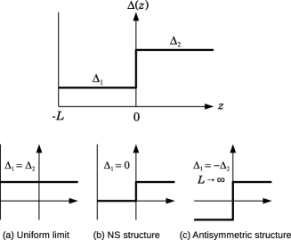
Figure 1: Model of nonuniform system. Upper panel: a spin-singlet $s$-wave pairing state occupying the semi-infinite space $-L<z$ with a specular surface at $z=-L$. Lower panel: three particular cases.

Using the quasiclassical theory of superconductivity,Serene-Rainer we can analyze the pair amplitude, the superfluid density, and the spin susceptibility in the region $z<0$ of the above model system. It is shown that the induced odd-frequency singlet pairing yields a negative pair density, as in the case of the odd-frequency triplet $s$-wave pairing. To investigate the odd-frequency pairing effect on the spin susceptibility, we generalize the Yosida formula (2) to the nonuniform singlet state. The resulting formula describes how the spin susceptibility is related to the even- and odd-frequency pair amplitudes. It is found from the generalized Yosida formula that the odd-frequency singlet pairs increase the spin susceptibility owing to the negative pair density.

Section II outlines the framework of the quasiclassical theory. In Sec. III, the quasiclassical theory is applied to the nonuniform system in Fig. 1 and explicit expressions for the even- and odd-frequency pair amplitudes in $z<0$ are derived. The odd-frequency pairing effect on the superfluid density is discussed in Sec. IV. The Meissner effect in NS proximity structures is also discussed in this section, with a focus on why the Meissner current is not induced in the proximity region of a clean N layer with infinitely large layer width.HigashitaniJPSJ1995 Finally, the spin susceptibility is analyzed in Sec. V.

II Quasiclassical theory

The quasiclassical theory is formulated in terms of a 4 $\times$ 4 matrix Green’s function $\hat{g}(\hat{p},\epsilon,\bm{r})$ in the Nambu space, where $\hat{p}$ is the unit vector specifying the direction of the Fermi momentum $\bm{p}_{F}=\hbar\bm{k}_{F}$ (and where a spherical Fermi surface is assumed below), $\epsilon$ is a complex energy variable, and $\bm{r}$ is the spatial coordinate. The quasiclassical Green’s function $\hat{g}$ obeys the Eilenberger equation

$$i\hbar v_{F}\hat{p}\cdot\nabla\hat{g}+[\hat{\epsilon}(\hat{p},\epsilon,\bm{r}),\ \hat{g}]=0$$ (4)

with the normalization condition $\hat{g}^{2}=-1$. In Eq. (4), $v_{F}$ is the Fermi velocity and $\hat{\epsilon}$ is an energy matrix of the form

$$\hat{\epsilon}(\hat{p},\epsilon,\bm{r})=\epsilon\hat{\rho}_{3}-\hat{v}(\hat{p},\bm{r})+\hat{\Delta}(\hat{p},\bm{r}),$$ (5)

where $\hat{\rho}_{3}$ is the third Pauli matrix in particle-hole space, $\hat{v}$ is a perturbation including Fermi liquid corrections, and $\hat{\Delta}$ is a mean field (gap function) resulting from Cooper pairing. In singlet pairing states, $\hat{\Delta}$ is expressed as

$$\hat{\Delta}(\hat{p},\bm{r})=\begin{bmatrix}0&\Delta(\hat{p},\bm{r})i\sigma_{2}\\ \Delta(\hat{p},\bm{r})^{*}i\sigma_{2}&0\\ \end{bmatrix}.$$ (6)

In the present work, the Fermi liquid corrections in $\hat{v}$ are neglected for simplicity. We can then determine the superfluid density and the spin susceptibility by calculating the linear response to the spatially uniform perturbation

$$\hat{v}(\hat{p})=v_{\hat{p}}\hat{\rho}_{3}-h\sigma_{3}\hat{1},$$ (7)

where $v_{\hat{p}}=p_{F}\hat{p}\cdot\bm{v}_{s}$, with $\bm{v}_{s}$ the superfluid velocity, $h=\mu_{0}H$ is the Zeeman coupling of the spin magnetic moment $\mu_{0}$ to the external field $H$, and $\hat{1}$ is the unit matrix in particle-hole space.

In the absence of the perturbation, the 4 $\times$ 4 energy matrix $\hat{\epsilon}$ for singlet states has the form

$$\hat{\epsilon}=\begin{bmatrix}\epsilon&0&0&\Delta\\ 0&\epsilon&-\Delta&0\\ 0&\Delta^{*}&-\epsilon&0\\ -\Delta^{*}&0&0&-\epsilon\end{bmatrix}.$$ (8)

The energy matrix $\hat{\epsilon}$ is separated into two $2\times 2$ subspaces (outer and inner subspaces). The singlet states can therefore be described by the $2\times 2$ matrix Eilenberger equation

$$i\hbar v_{F}\hat{p}\cdot\nabla\hat{g}_{2\times 2}+[\hat{\epsilon}_{2\times 2}(\hat{p},\epsilon,\bm{r}),\ \hat{g}_{2\times 2}]=0$$ (9)

with

$$\hat{\epsilon}_{2\times 2}(\hat{p},\epsilon,\bm{r})=\begin{bmatrix}\epsilon&\Delta(\hat{p},\bm{r})\\ -\Delta(\hat{p},\bm{r})^{*}&-\epsilon\\ \end{bmatrix}.$$ (10)

The perturbation shifts the energy variable $\epsilon$, and the quasiclassical Green’s functions in the outer and inner subspaces are given by

$$\hat{g}_{\rm outer}=\hat{g}_{2\times 2}(\hat{p},\epsilon-v_{\hat{p}}+h,\bm{r}),$$ (11)

$$\hat{g}_{\rm inner}=\hat{\rho}_{3}\hat{g}_{2\times 2}(\hat{p},\epsilon-v_{\hat{p}}-h,\bm{r})\hat{\rho}_{3}.$$ (12)

The Green’s function $\hat{g}_{2\times 2}$ has the matrix structure

$$\hat{g}_{2\times 2}(\hat{p},\epsilon,\bm{r})=\begin{bmatrix}g(\hat{p},\epsilon,\bm{r})&f(\hat{p},\epsilon,\bm{r})\\ -\widetilde{f}(\hat{p},\epsilon,\bm{r})&-g(\hat{p},\epsilon,\bm{r})\end{bmatrix},$$ (13)

where

$$\widetilde{f}(\hat{p},\epsilon,\bm{r})=f(-\hat{p},-\epsilon^{*},\bm{r})^{*}.$$ (14)

The diagonal and off-diagonal elements have the symmetries

$$g(\hat{p},\epsilon,\bm{r})=g(\hat{p},\epsilon^{*},\bm{r})^{*},$$ (15)

$$f(\hat{p},\epsilon,\bm{r})=f(-\hat{p},-\epsilon,\bm{r}).$$ (16)

The function $g$ carries information on quasiparticle excitation. The local density of states is calculated from $g$ as

$$\begin{split}n(\hat{p},E,\bm{r})&={\rm Im}[g(\hat{p},E+i0,\bm{r})]\\ &=\frac{1}{2i}[g(\hat{p},E+i0,\bm{r})-g(\hat{p},E-i0,\bm{r})],\end{split}$$ (17)

where $E$ is a real energy variable. By using $g$ in the Matsubara representation ($\epsilon=i\epsilon_{n}$), the supercurrent $\bm{J}(\bm{r})$ and the spin magnetization $M(\bm{r})$ are obtained from

$$\bm{J}(\bm{r})=-2N(0)v_{F}\frac{\pi}{\beta}\sum_{\epsilon_{n}}\left\langle\hat{p}\,g(\hat{p},i\epsilon_{n}-v_{\hat{p}},\bm{r})\right\rangle_{\hat{p}},$$ (18)

$$\frac{M(\bm{r})}{\chi_{0}H}=1-\frac{1}{h}\frac{\pi}{\beta}\sum_{\epsilon_{n}}\sum_{\sigma=\pm}\left\langle\frac{\sigma}{2}\,g(\hat{p},i\epsilon_{n}+\sigma h,\bm{r})\right\rangle_{\hat{p}},$$ (19)

where $N(0)$ is the density of states per spin at the Fermi level in the normal state and $\chi_{0}=2N(0)\mu_{0}^{2}$ is the susceptibility in the normal state.

The function $f$ corresponds to the singlet pair amplitude defined on the complex $\epsilon$ plane. Equation (16) represents a general symmetry relation for $f$, showing that an even-parity (odd-parity) singlet pair amplitude has even-frequency (odd-frequency) symmetry.

A more explicit expression for $\hat{g}_{\rm 2\times 2}$ can be obtained by expressing it in the form

$$\hat{g}_{\rm 2\times 2}=\frac{2i}{\left\langle\bm{r}\right|\left.\!\!\bm{r}\right\rangle}\left|\bm{r}\right\rangle\left\langle\bm{r}\right|-i,$$ (20)

where $\left|\bm{r}\right\rangle$ and $\left\langle\bm{r}\right|$ are the column and row vectors satisfying

$$i\hbar v_{F}\hat{p}\cdot\nabla\left|\bm{r}\right\rangle =-\hat{\epsilon}_{2\times 2}(\hat{p},\epsilon,\bm{r})\left|\bm{r}\right\rangle,$$ (21)

$$i\hbar v_{F}\hat{p}\cdot\nabla\left\langle\bm{r}\right| =\left\langle\bm{r}\right|\hat{\epsilon}_{2\times 2}(\hat{p},\epsilon,\bm{r}).$$ (22)

Noting that $\left\langle\bm{r}\right|\left.\!\!\bm{r}\right\rangle$ is independent of $\bm{r}$, we can easily show that $\hat{g}_{\rm 2\times 2}$ of Eq. (20) satisfies the Eilenberger equation (9) with the normalization condition $\hat{g}_{\rm 2\times 2}^{2}=-1$. The column and row vectors can be parameterized as

$$\left|\bm{r}\right\rangle=a\begin{bmatrix}1\\ \widetilde{\mathcal{F}}\end{bmatrix},\quad\left\langle\bm{r}\right|=a^{\prime}\begin{bmatrix}1&\mathcal{F}\end{bmatrix}.$$ (23)

Substitution of Eq. (23) into Eq. (20) yields the following parameterization for $\hat{g}_{2\times 2}$:

$$\hat{g}_{2\times 2}+i=\frac{2i}{1+\mathcal{F}\widetilde{\mathcal{F}}}\begin{bmatrix}1\\ \widetilde{\mathcal{F}}\end{bmatrix}\begin{bmatrix}1&\mathcal{F}\end{bmatrix}.$$ (24)

The functions $\mathcal{F}$ and $\widetilde{\mathcal{F}}$ satisfy the Riccati-type differential equations

$$i\hbar v_{F}\hat{p}\cdot\nabla\mathcal{F} =-2\epsilon\mathcal{F}+\Delta(\hat{p},\bm{r})+\Delta(\hat{p},\bm{r})^{*}\mathcal{F}^{2},$$ (25)

$$i\hbar v_{F}\hat{p}\cdot\nabla\widetilde{\mathcal{F}} =2\epsilon\widetilde{\mathcal{F}}+\Delta(\hat{p},\bm{r})^{*}+\Delta(\hat{p},\bm{r})\widetilde{\mathcal{F}}^{2}.$$ (26)

In bulk systems with a constant gap function $\Delta(\hat{p})$, the Riccati equations have solutions

$$\mathcal{F}^{\rm bulk}=\frac{\Delta(\hat{p})}{\epsilon+i\sqrt{|\Delta(\hat{p})|^{2}-\epsilon^{2}}},$$ (27)

$$\widetilde{\mathcal{F}}^{\rm bulk}=-\frac{\Delta(\hat{p})^{*}}{\epsilon+i\sqrt{|\Delta(\hat{p})|^{2}-\epsilon^{2}}}.$$ (28)

Substituting Eqs. (27) and (28) into Eq. (24), we obtain the well-known bulk solution of $\hat{g}_{2\times 2}$, i.e.,

$$\hat{g}_{2\times 2}^{\rm bulk}(\hat{p},\epsilon)=\frac{1}{\sqrt{|\Delta(\hat{p})|^{2}-\epsilon^{2}}}\begin{bmatrix}\epsilon&\Delta(\hat{p})\\ -\Delta(\hat{p})^{*}&-\epsilon\\ \end{bmatrix}.$$ (29)

One can show from Eqs. (25)–(28) that $\widetilde{\mathcal{F}}$ is related to $\mathcal{F}$ by the transformation

$$\widetilde{\mathcal{F}}(\hat{p},\epsilon,\bm{r})=\mathcal{F}(-\hat{p},-\epsilon^{*},\bm{r})^{*}.$$ (30)

Moreover, $\mathcal{F}$ and $\widetilde{\mathcal{F}}$ are found to have the symmetries

$$\mathcal{F}(\hat{p},\epsilon,\bm{r})={1}/{\mathcal{F}(\hat{p},\epsilon^{*},\bm{r})^{*}},$$ (31)

$$\widetilde{\mathcal{F}}(\hat{p},\epsilon,\bm{r})={1}/{\widetilde{\mathcal{F}}(\hat{p},\epsilon^{*},\bm{r})^{*}}.$$ (32)

Equations (31) and (32) can be used to check the Green’s function symmetries of Eqs. (15) and (16).

III Pair amplitude

We now consider the model system in Fig. 1. The function $\mathcal{F}$ obeys

$$i\hbar v_{F}\hat{p}_{z}\partial_{z}\mathcal{F}=-2\epsilon\mathcal{F}+\Delta(z)(1+\mathcal{F}^{2})$$ (33)

with the following boundary conditions: (i) $\mathcal{F}\to\mathcal{F}^{\rm bulk}$ at $z\to\infty$, (ii) $\mathcal{F}$ is continuous at $z=0$, and (iii) $\mathcal{F}$ satisfies the specular-surface boundary condition $\mathcal{F}(\hat{p}_{z})=\mathcal{F}(-\hat{p}_{z})$ at $z=-L$.

Since $\Delta(z)$ is a real function, $\mathcal{F}$ has the symmetry

$$\mathcal{F}(\hat{p},\epsilon,z)=-\mathcal{F}(\hat{p},-\epsilon^{*},z)^{*}.$$ (34)

The corresponding symmetry for the pair amplitude is

$$f(\hat{p},\epsilon,z)=f(\hat{p},-\epsilon^{*},z)^{*}.$$ (35)

This shows that $f$ for $\epsilon=i\epsilon_{n}$ is a real quantity.

In general, the pair amplitude has even-frequency (EF) and odd-frequency (OF) components,

$$f(\hat{p},\epsilon,z)=f^{\rm EF}(\hat{p},\epsilon,z)+f^{\rm OF}(\hat{p},\epsilon,z).$$ (36)

Combining the symmetries (35) and (16), we find that $\widetilde{f}$ can be decomposed as

$$\widetilde{f}(\hat{p},\epsilon,z)=f^{\rm EF}(\hat{p},\epsilon,z)-f^{\rm OF}(\hat{p},\epsilon,z).$$ (37)

In the model system, we can solve analytically the Riccati equation (33). The general solution can be written in the form

$$\mathcal{F}(z<0)=\frac{\mathcal{F}_{1}+C_{1}e^{-s_{p}\kappa_{1}z}}{1+\mathcal{F}_{1}C_{1}e^{-s_{p}\kappa_{1}z}},$$ (38)

$$\mathcal{F}(z>0)=\frac{\mathcal{F}_{2}+C_{2}e^{-s_{p}\kappa_{2}z}}{1+\mathcal{F}_{2}C_{2}e^{-s_{p}\kappa_{2}z}},$$ (39)

where

$$\mathcal{F}_{i}=\frac{\Delta_{i}}{\epsilon+i\sqrt{\Delta_{i}^{2}-\epsilon^{2}}}\ \ (i=1,2),$$ (40)

$$\kappa_{i}=\frac{2\sqrt{\Delta_{i}^{2}-\epsilon^{2}}}{\hbar v_{F}|\hat{p}_{z}|},$$ (41)

$$s_{p}={\rm sgn}(\hat{p}_{z}),$$ (42)

and $C_{i}$s are constants to be determined from the boundary conditions. Imposing the boundary conditions, we obtain

$$\mathcal{F}(z<0) =\frac{1+s_{p}}{2}\frac{\mathcal{F}_{1}+Ce^{-\kappa_{1}(z+2L)}}{1+\mathcal{F}_{1}Ce^{-\kappa_{1}(z+2L)}}$$

$$+\frac{1-s_{p}}{2}\frac{\mathcal{F}_{1}+Ce^{\kappa_{1}z}}{1+\mathcal{F}_{1}Ce^{\kappa_{1}z}},$$ (43)

$$\mathcal{F}(z>0) =\frac{1+s_{p}}{2}\frac{\mathcal{F}_{2}-C^{\prime}e^{-\kappa_{2}z}}{1-\mathcal{F}_{2}C^{\prime}e^{-\kappa_{2}z}}$$

$$+\frac{1-s_{p}}{2}\mathcal{F}_{2},$$ (44)

where

$$C=\frac{\mathcal{F}_{2}-\mathcal{F}_{1}}{1-\mathcal{F}_{1}\mathcal{F}_{2}},\quad C^{\prime}=\frac{C(1-e^{-2\kappa_{1}L})}{1-C^{2}e^{-2\kappa_{1}L}}.$$ (45)

The factors $(1+s_{p})/2$ and $(1-s_{p})/2$ in Eqs. (43) and (44) select $\mathcal{F}$ with $\hat{p}_{z}>0$ and with $\hat{p}_{z}<0$, respectively.

In what follows, we shall focus on the region $z<0$. Using Eq. (43), we find that the quasiclassical Green’s function $\hat{g}_{2\times 2}$ in $z<0$ is given as

$$\hat{g}_{2\times 2}(z<0)+i =\frac{(1+s_{p})i}{D}\biggl{(}\begin{bmatrix}1\\ -\mathcal{F}_{1}\end{bmatrix}+Ce^{\kappa_{1}z}\begin{bmatrix}\mathcal{F}_{1}\\ -1\end{bmatrix}\biggr{)}\biggl{(}\begin{bmatrix}1&\mathcal{F}_{1}\end{bmatrix}+Ce^{-\kappa_{1}(z+2L)}\begin{bmatrix}\mathcal{F}_{1}&1\end{bmatrix}\biggr{)}$$

$$+\frac{(1-s_{p})i}{D}\biggl{(}\begin{bmatrix}1\\ -\mathcal{F}_{1}\end{bmatrix}+Ce^{-\kappa_{1}(z+2L)}\begin{bmatrix}\mathcal{F}_{1}\\ -1\end{bmatrix}\biggr{)}\biggl{(}\begin{bmatrix}1&\mathcal{F}_{1}\end{bmatrix}+Ce^{\kappa_{1}z}\begin{bmatrix}\mathcal{F}_{1}&1\end{bmatrix}\biggr{)}$$ (46)

with $D=(1-\mathcal{F}_{1}^{2})(1-C^{2}e^{-2\kappa_{1}L})$.

Equation (46) depends on $\Delta_{2}$ via the constant $C$. When $\Delta_{1}=\Delta_{2}$ (the uniform limit), $C$ vanishes and then Eq. (46) is reduced to the bulk solution, as expected from the fact that the $s$-wave pairing state is not affected by surface scattering. However, the spatial inhomogeneity arising from $\Delta_{1}\neq\Delta_{2}$ makes $C$ finite. For example, in the NS structure, we have $\mathcal{F}_{1}=0$ for $\epsilon=E+i0$ and then $C=\mathcal{F}_{2}$. Note that, in this case, Eq. (46) for $\hat{p}_{z}>0$ and $L\to\infty$ can be expressed in the form

$$\hat{g}_{2\times 2}(z<0)+i=2i\hat{\rho}_{3}\left(\begin{bmatrix}1\\ 0\end{bmatrix}e^{iqz}+\mathcal{F}_{2}\begin{bmatrix}0\\ 1\end{bmatrix}e^{-iqz}\right)\begin{bmatrix}1&0\end{bmatrix}e^{-iqz},$$ (47)

where $q=E/\hbar v_{F}|\hat{p}_{z}|$. The two column vectors on the right-hand side of Eq. (47) represent the Andreev scattering process in N of the NS structure. This shows that $\mathcal{F}_{2}$ for real energies gives the Andreev reflection amplitude.

The upper-right matrix element of Eq. (46) gives the pair amplitude $f$ in $z<0$. In the expression for $f$, the terms $\propto s_{p}$ are odd-parity pair amplitudes and therefore have OF symmetry. We can check the frequency symmetry using the relation $\mathcal{F}_{i}(-\epsilon)=-\mathcal{F}_{i}^{-1}(\epsilon)$ ($i=1,2$). We thus find that in the region $z<0$ there coexist EF and OF pairs with amplitudes

$$f^{\rm EF}(\hat{p},\epsilon,z<0)=i\,\frac{2\mathcal{F}_{1}\left(1+C^{2}e^{-2\kappa_{1}L}\right)+(1+\mathcal{F}_{1}^{2})C\left(e^{\kappa_{1}z}+e^{-\kappa_{1}(z+2L)}\right)}{(1-\mathcal{F}_{1}^{2})\left(1-C^{2}e^{-2\kappa_{1}L}\right)},$$ (48)

$$f^{\rm OF}(\hat{p},\epsilon,z<0)=-s_{p}i\,\frac{C\left(e^{\kappa_{1}z}-e^{-\kappa_{1}(z+2L)}\right)}{1-C^{2}e^{-2\kappa_{1}L}},$$ (49)

respectively. The OF pair amplitude is proportional to $C$. This means that it vanishes in the uniform limit and then the EF pair amplitude takes the bulk form $f^{\rm bulk}=\Delta_{1}/\sqrt{\Delta_{1}^{2}-\epsilon^{2}}$.

When $\Delta_{1}=0$ (NS structure), the EF and OF pairs for $\epsilon=E+i0$ have amplitudes

$$f^{\rm EF}(\hat{p},\epsilon,z<0)=i\,\frac{\mathcal{F}_{2}\left(e^{\kappa_{1}z}+e^{-\kappa_{1}(z+2L)}\right)}{1-\mathcal{F}_{2}^{2}e^{-2\kappa_{1}L}},$$ (50)

$$f^{\rm OF}(\hat{p},\epsilon,z<0)=-s_{p}i\,\frac{\mathcal{F}_{2}\left(e^{\kappa_{1}z}-e^{-\kappa_{1}(z+2L)}\right)}{1-\mathcal{F}_{2}^{2}e^{-2\kappa_{1}L}},$$ (51)

respectively. The pair amplitudes are proportional to the Andreev reflection amplitude $\mathcal{F}_{2}$. The denominator with $\mathcal{F}_{2}$ describes the multiple Andreev scattering effect in an N layer of finite width $L$. Equations (50) and (51) can also be applied to the case of $\epsilon=i\epsilon_{n}$ with $\epsilon_{n}>0$. Then, the spatial dependence of the pair amplitudes is characterized by

$$\kappa_{1}=\frac{2|\epsilon_{n}|}{\hbar v_{F}|\hat{p}_{z}|}=\frac{|2n+1|}{\xi_{N}(T)|\hat{p}_{z}|}$$ (52)

with $\xi_{N}(T)=\hbar v_{F}/2\pi k_{B}T$ being the coherence length in the N layer. The Matsubara pair amplitudes in the N layer decay exponentially from $z=0$ and penetrate to a distance $\sim\xi_{N}(T)$. The EF and OF pair amplitudes have the same magnitude in the limit $L/\xi_{N}(T)\gg 1$. This is because in that limit the total propagator $f$ with $\hat{p}_{z}>0$ does not carry information on the proximity effect, i.e., $f(\hat{p},\epsilon,z<0)=0$ for $\hat{p}_{z}>0$.

Let us consider infinite systems with $\Delta_{1}\neq 0$. Taking the limit $L\to\infty$ in Eqs. (48) and (49), we obtain

$$f^{\rm EF}(\hat{p},\epsilon,z<0)=i\,\frac{2\mathcal{F}_{1}+(1+\mathcal{F}_{1}^{2})Ce^{\kappa_{1}z}}{1-\mathcal{F}_{1}^{2}},$$ (53)

$$f^{\rm OF}(\hat{p},\epsilon,z<0)=-s_{p}i\,Ce^{\kappa_{1}z}.$$ (54)

It should be noted here that $C$ diverges at $\epsilon=0$ when ${\rm sgn}(\Delta_{1}\Delta_{2})<0$. This corresponds to the pole of the midgap Andreev bound states localized around $z=0$. The OF pair amplitude has the midgap-state pole, whereas the EF pair amplitude does not, because $1+\mathcal{F}_{1}^{2}\propto\epsilon$ in the low-energy limit. As shall be shown in the Appendix, the midgap (zero-energy) density of states can be written in terms of the OF pair amplitude.

In the particular case of $L\to\infty$ and $\Delta_{1}=-\Delta_{2}$ (antisymmetric structure), we get from Eqs. (53) and (54) the following explicit expressions for the EF and OF pair amplitudes:

$$f^{\rm EF}(\hat{p},\epsilon,z<0) =\frac{\Delta_{1}}{\sqrt{\Delta_{1}^{2}-\epsilon^{2}}}(1-e^{\kappa_{1}z}),$$ (55)

$$f^{\rm OF}(\hat{p},\epsilon,z<0) =s_{p}\frac{i\Delta_{1}}{\epsilon}e^{\kappa_{1}z}.$$ (56)

In this case, the total pair amplitude at $z=0$ is dominated by the OF pairs.

IV Superfluid density

In the system considered above, supercurrent can flow along the surface (perpendicular to the $z$ axis). The corresponding superfluid density can be obtained by calculating the linear response of $g$ to $v_{\hat{p}}=p_{F}\hat{p}_{x}v_{s}$. The linear deviation $\delta g$ of the Matsubara $g$ function is given as

$$\delta g(\hat{p},i\epsilon_{n}-v_{\hat{p}},z)=-v_{\hat{p}}\,g^{\prime}(\hat{p},i\epsilon_{n},z)$$ (57)

with

$$g^{\prime}(\hat{p},i\epsilon_{n},z)=(-i)\frac{\partial}{\partial\epsilon_{n}}g(\hat{p},i\epsilon_{n},z).$$ (58)

Equation (58) relates explicitly the response function $g^{\prime}$ to the unperturbed Green’s function $g$. Such a definition of $g^{\prime}$ is, however, not so convenient for the analysis of the Cooper pairing effect on the superfluid density. A more useful formula can be obtained by starting with Eq. (24), giving the expression

$$g+i=\frac{2i}{1+\mathcal{F}\widetilde{\mathcal{F}}}.$$ (59)

Let $\delta\mathcal{F}$ be the linear deviation of $\mathcal{F}$. Replacing $\mathcal{F}$ in Eq. (59) by $\mathcal{F}+\delta\mathcal{F}$, we obtain

$$\delta g=-v_{\hat{p}}\,g^{\prime}=-\frac{2i}{(1+\mathcal{F}\widetilde{\mathcal{F}})^{2}}(\delta\mathcal{F}\widetilde{\mathcal{F}}+\mathcal{F}\delta\widetilde{\mathcal{F}}).$$ (60)

Moreover, using the expression

$$f=\frac{2i\mathcal{F}}{1+\mathcal{F}\widetilde{\mathcal{F}}}$$ (61)

for the pair amplitude, we get the following formula for the response function:

$$g^{\prime}(\hat{p},i\epsilon_{n},z)=\Lambda(\hat{p},i\epsilon_{n},z)f(\hat{p},i\epsilon_{n},z)\widetilde{f}(\hat{p},i\epsilon_{n},z)$$ (62)

with

$$\Lambda(\hat{p},i\epsilon_{n},z)=-\frac{1}{2iv_{\hat{p}}}\left\{\frac{\delta\mathcal{F}}{\mathcal{F}}+\frac{\delta\widetilde{\mathcal{F}}}{\widetilde{\mathcal{F}}}\right\}{(\hat{p},i\epsilon_{n},z)}.$$ (63)

In Eq. (63), the notation $\{\cdots\}{(\hat{p},i\epsilon_{n},z)}$ denotes that all the functions in the curly braces have the same argument $(\hat{p},i\epsilon_{n},z)$.

From Eqs. (62), (57), and (18), we find that the superfluid fraction is given by

$$\frac{n_{s}(z)}{n}=\frac{\pi}{\beta}\sum_{\epsilon_{n}}\left\langle 3\hat{p}_{x}^{2}\left\{\Lambda P\right\}{(\hat{p},i\epsilon_{n},z)}\right\rangle_{\hat{p}}$$ (64)

with

$$P=f\widetilde{f}=(f^{\rm EF})^{2}-(f^{\rm OF})^{2}.$$ (65)

Since $f$ with $\epsilon=i\epsilon_{n}$ is a real function, $P(\hat{p},i\epsilon_{n},z)$ is a real quantity. The function $\Lambda(\hat{p},i\epsilon_{n},z)$ is also a real quantity because $\mathcal{F}$ and $\delta\mathcal{F}$ in the Matsubara representation are purely imaginary and real, respectively. Moreover, one can show that $\Lambda$ has the symmetry

$$\Lambda(\hat{p},i\epsilon_{n},z)=\Lambda(-\hat{p},i\epsilon_{n},z)=\Lambda(\hat{p},-i\epsilon_{n},z).$$ (66)

Namely, $\Lambda$ is even in $\hat{p}$ and in $\epsilon_{n}$.

It is instructive to compare Eq. (64) with the corresponding formula for a dirty singlet superconductor, i.e., Eq. (1). The superfluid fraction in the dirty system is obtained by the replacement

$$\Lambda\to 2\tau_{\rm tr}/\hbar,\quad P\to(f^{\rm EF}_{\rm SW})^{2},$$ (67)

where $f^{\rm EF}_{\rm SW}$ denotes the even-frequency $s$-wave pair amplitude. Note that $\hbar v_{F}\Lambda/2$ coincides with the mean free path $v_{F}\tau_{\rm tr}$. This implies that the quantity $\hbar v_{F}\Lambda/2$ corresponds to the range of the linear response kernel; in other words, $n_{s}(z)$ is determined depending only on $\bm{v}_{s}$ in the region of width $\sim\hbar v_{F}\Lambda/2$ around position $z$. The pair density $P$ in the dirty singlet superconductor does not contain the OF pair amplitude. This is because impurity scattering destroys non-$s$-wave pairs and singlet $s$-wave pairing has even-frequency symmetry.

However, in the clean systems under consideration, the OF pairs exist except at the uniform limit. Equation (65) shows that the OF pairing yields a negative pair density.

The rest of this section is devoted to a discussion of the superfluid density in the three particular clean system cases: the uniform limit [Fig. 1(a)], the NS structure [Fig. 1(b)], and the antisymmetric structure [Fig. 1(c)].

IV.1 Uniform limit

In the case of $\Delta_{1}=\Delta_{2}\equiv\Delta$, we have

$$\mathcal{F}=\mathcal{F}^{\rm bulk},\quad f^{\rm EF}=f^{\rm bulk},\quad f^{\rm OF}=0.$$ (68)

Using

$$\frac{\partial\mathcal{F}^{\rm bulk}}{\partial\epsilon_{n}}=\frac{\partial}{\partial\epsilon_{n}}\frac{-i\Delta}{\epsilon_{n}+\sqrt{\Delta^{2}+\epsilon_{n}^{2}}}=-\frac{\mathcal{F}^{\rm bulk}}{\sqrt{\Delta^{2}+\epsilon_{n}^{2}}},$$ (69)

we can obtain

$$\Lambda=\frac{1}{\sqrt{\Delta^{2}+\epsilon_{n}^{2}}}.$$ (70)

Note that $\hbar v_{F}\Lambda/2$ coincides with the $\epsilon_{n}$-dependent coherence length $\xi(\epsilon_{n},\Delta)=\hbar v_{F}/2\sqrt{\Delta^{2}+\epsilon_{n}^{2}}$ , which determines the range of the linear response kernel in the clean superconductor with gap $\Delta$. The pair density in the uniform superconductor is

$$P=(f^{\rm bulk})^{2}=\frac{\Delta^{2}}{\Delta^{2}+\epsilon_{n}^{2}}.$$ (71)

Substitution of Eqs. (70) and (71) into Eq. (64) leads to

$$\frac{n_{s}}{n}=\frac{\pi}{\beta}\sum_{\epsilon_{n}}\frac{\Delta^{2}}{(\Delta^{2}+\epsilon_{n}^{2})^{3/2}},$$ (72)

which is the well-known result for the superfluid fraction in clean bulk $s$-wave superconductors.

IV.2 NS structure

This subsection focuses on the N layer of the NS structure.

In the clean N layer, the superfluid density is known to take a spatially constant value despite the existence of the spatially varying pair amplitude. This property can be readily shown from the Eilenberger equation in the normal state,

$$i\hbar v_{F}\hat{p}_{z}\partial_{z}\hat{g}_{2\times 2}^{N}+[(i\epsilon_{n}-v_{\hat{p}})\hat{\rho}_{3},\ \hat{g}_{2\times 2}^{N}]=0.$$ (73)

The spatial dependence of $\hat{g}_{2\times 2}^{N}(z)$ is described by

$$\hat{g}_{2\times 2}^{N}(z)=e^{-\kappa_{N}(z-z^{\prime})\hat{\rho}_{3}}\hat{g}_{2\times 2}^{N}(z^{\prime})e^{\kappa_{N}(z-z^{\prime})\hat{\rho}_{3}}$$ (74)

with $\kappa_{N}=(\epsilon_{n}+iv_{\hat{p}})/\hbar v_{F}\hat{p}_{z}$. It follows that the diagonal element $g^{N}(z)$ of $\hat{g}_{2\times 2}^{N}(z)$ is independent of $z$. This also means that the Meissner response of the clean N layer is completely nonlocal.HigashitaniJPSJ1995

From the $n_{s}$ formula (64), the superfluid density in the N layer is obtained as follows. The function $\Lambda$ is determined from Eq. (43) with $\mathcal{F}_{1}=0$ and $\kappa_{1}=2|\epsilon_{n}|/\hbar v_{F}|\hat{p}_{z}|$. The result is

$$\Lambda=\frac{2L}{\hbar v_{F}|\hat{p}_{z}|}+\frac{1}{\sqrt{\Delta_{2}^{2}+\epsilon_{n}^{2}}}.$$ (75)

The first term is proportional to $L$ because of the nonlocal response of the clean N layer. The second term implies that the N-side superfluid density includes information on $\bm{v}_{s}$ in the region of $0<z\lesssim\xi(\epsilon_{n},\Delta_{2})$ on the S side. The pair density $P$ in the N layer is obtained from Eqs. (50) and (51) as

$$P=(f^{\rm EF})^{2}-(f^{\rm OF})^{2}=\left|\frac{2\mathcal{F}_{2}}{1-\mathcal{F}_{2}^{2}e^{-2\kappa_{1}L}}\right|^{2}e^{-2\kappa_{1}L}.$$ (76)

The spatially dependent terms in $(f^{\rm EF})^{2}$ and $(f^{\rm OF})^{2}$ cancel out in $P$.

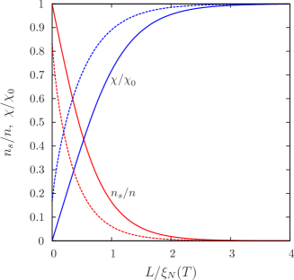
Figure 2: (Color online) $n_{s}/n$ and $\chi/\chi_{0}$ in the clean N layer of the NS structure as a function of $L/\xi_{N}(T)$. The solid lines are the results for $T/T_{c}=0.1$ and the dashed lines are for $T/T_{c}=0.5$ (where $T_{c}$ is the transition temperature of the superconductor).

In Fig. 2, the superfluid fraction $n_{s}/n$ in the N layer is plotted as a function of $L$ scaled by $\xi_{N}(T)$ at given reduced temperatures $T/T_{c}=0.1$ and 0.5. In the limit $L\to 0$, the superfluid fraction coincides with that in the uniform state with gap $\Delta_{2}$. As $L$ increases, $n_{s}/n$ decreases and becomes exponentially small for $L\gg\xi_{N}(T)$. In the limit $L/\xi_{N}(T)\to\infty$, the superfluid density vanishes because $|f^{\rm OF}|$ is then equal to $|f^{\rm EF}|$ and consequently $P=0$.

The vanishing superfluid density in the clean N layer for $L/\xi_{N}(T)\gg 1$ has been noted in a study of the Meissner effect in NS structures.HigashitaniJPSJ1995 Mathematically, this is a consequence of $g^{N}(z)$ being constant and therefore being equal to the normal-state value everywhere in an N layer of infinitely large layer width. The question, however, remains as to why supercurrent does not flow even in the proximity region with a finite pair amplitude. The present theory provides the following answer: because the pair density associated with OF pairing is negative, the supercurrent carried by OF pairs flows in the opposite direction to $\bm{v}_{s}$ and compensates for the conventional supercurrent carried by EF pairs.

In dirty systems, in contrast, the OF singlet pairs are destroyed by impurity scattering. As a result, the dirty N layer exhibits a (diamagnetic) Meissner effect similar to that in conventional superconductors. The diamagnetic Meissner current also flows in the clean N layer when $L/\xi_{N}(T)\lesssim 1$. In this case, imbalance between $|f^{\rm EF}|$ and $|f^{\rm OF}|$ ($|f^{\rm EF}|>|f^{\rm OF}|$) is caused by surface scattering.

IV.3 Antisymmetric structure

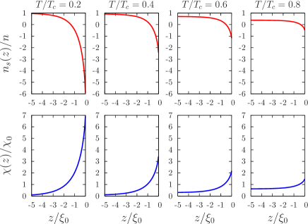
Figure 3: (Color online) Spatial dependence of $n_{s}(z<0)/n$ and $\chi(z<0)/\chi_{0}$ in the antisymmetric structure at $T/T_{c}=0.2$, 0.4, 0.6, and 0.8.

We now turn to the antisymmetric structure. Plotted in the upper part of Fig. 3 is $n_{s}(z<0)/n$ in the antisymmetric structure as a function of $z/\xi_{0}$, where $\xi_{0}=\hbar v_{F}/2\pi k_{B}T_{c}$. The superfluid density $n_{s}(z)$ depends strongly on position $z$, unlike that in the N layer of the NS system. In the antisymmetric structure, $n_{s}(z)$ has the bulk value in the region $z\ll-\xi_{0}$ but takes a negative value around $z=0$. The magnitude of the negative superfluid density at $z=0$ increases with decreasing temperature $T$.

Let us discuss $n_{s}(z=0)$. The function $\Lambda$ at $z=0$ has the form

$$\Lambda(z=0)=\frac{1}{2}\sum_{i=1,2}\frac{1}{\sqrt{\Delta_{i}^{2}+\epsilon_{n}^{2}}}=\frac{1}{\sqrt{\Delta_{1}^{2}+\epsilon_{n}^{2}}}.$$ (77)

The pair density at $z=0$ is dominated by the OF pairs and takes the negative value

$$P(z=0)=-\frac{\Delta_{1}^{2}}{\epsilon_{n}^{2}}.$$ (78)

The resulting superfluid density at $z=0$ is

$$\frac{n_{s}(0)}{n}=-\frac{\pi}{\beta}\sum_{\epsilon_{n}}\frac{\Delta_{1}^{2}}{\epsilon_{n}^{2}\sqrt{\Delta_{1}^{2}+\epsilon_{n}^{2}}}<0.$$ (79)

Equation (79) predicts the temperature dependence of $n_{s}(0)/n$ as shown in the upper-left panel of Fig. 4. The superfluid fraction has a large negative value at low temperatures and diverges in the $T\to 0$ limit. It is obvious that the low-temperature divergence is due to the midgap-state pole of the OF pair amplitude $f^{\rm OF}$. Strictly, however, $n_{s}(0)/n$ does not diverge. The divergence is due to the breakdown of linear response theory at low temperatures. To demonstrate this, the low-temperature behavior of $J(z=0)/nv_{s}$ calculated from the general current formula (18) with $p_{F}v_{s}/k_{B}T_{c}=0.05$ is plotted with a dotted line in the upper-right panel of Fig. 4. The dotted line deviates from the linear response result (solid line) below $T/T_{c}\sim p_{F}v_{s}/k_{B}T_{c}$.

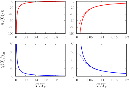
Figure 4: (Color online) Temperature dependence of $n_{s}(z)/n$ and $\chi(z)/\chi_{0}$ at $z=0$ in the antisymmetric structure. In the calculations, $\Delta_{1}$ is assumed to have the same temperature dependence as that of the bulk $s$-wave gap. The solid lines are the results from linear response theory. The dotted lines are the full numerical results obtained from the current formula (18) with $p_{F}v_{s}/k_{B}T_{c}=0.05$ and the magnetization formula (19) with $\mu_{0}H/k_{B}T_{c}=0.05$. The right panels demonstrate the breakdown of linear response theory at low temperatures below $\sim\negthickspace p_{F}v_{s}/k_{B}$ or $\sim\negthickspace\mu_{0}H/k_{B}$.

The origin of the deviation can be understood by expressing Eq. (18) in terms of the local density of states, $n(\hat{p},E,z)$,

$$J(z)=2N(0)v_{F}\int_{-\infty}^{\infty}dE\,n_{F}(E)\left\langle\hat{p}_{x}\,n(\hat{p},E_{\hat{p}},z)\right\rangle_{\hat{p}}.$$ (80)

Here, $E_{\hat{p}}=E-v_{\hat{p}}$ and $n_{F}(E)=1/(e^{\beta E}+1)$ is the Fermi function. The midgap-state pole of $f^{\rm OF}$ yields the zero-energy peak in the local density of states at $z=0$ (see the Appendix),

$$n_{\rm midgap}(\hat{p},E,0)=\pi|\Delta_{1}|\delta(E).$$ (81)

The contribution from the midgap states to $J(0)$ is evaluated to be

$$J_{\rm midgap}(0)=2N(0)v_{F}\pi|\Delta_{1}|\left\langle\hat{p}_{x}n_{F}(v_{\hat{p}})\right\rangle_{\hat{p}}.$$ (82)

Taking the $T\to 0$ limit, we obtain

$$J_{\rm midgap}(0)\xrightarrow{T\to 0}-\frac{1}{2}N(0)v_{F}\pi|\Delta_{1}|=-n\frac{3\pi|\Delta_{1}|}{4p_{F}}.$$ (83)

This result is independent of $v_{s}$ and suggests the breakdown of linear response theory. Since $n_{F}(v_{\hat{p}})$ in Eq. (82) cannot be expanded in powers of $v_{\hat{p}}$ at low temperatures $k_{B}T\lesssim p_{F}v_{s}$, linear response theory does not give the correct value of the midgap-state current at $T=0$. Linear response theory can still be used to evaluate the contribution from continuum states. At $T=0$, the continuum states carry the supercurrent $nv_{s}$. Adding the two contributions, we find that

$$J(0)\xrightarrow{T\to 0}n\left(v_{s}-\frac{3\pi|\Delta_{1}|}{4p_{F}}\right).$$ (84)

We see that the superfluid fraction defined as $J(0)/nv_{s}$ takes the zero-temperature value

$$1-\frac{3\pi|\Delta_{1}|}{4p_{F}v_{s}}\simeq-\frac{3\pi|\Delta_{1}|}{4p_{F}v_{s}},$$

which is finite, though it has a large negative value for small $v_{s}$, as suggested by linear response theory.

Equation (83) shows that the magnitude of $J_{\rm midgap}$ is as large as the critical current density $\sim n|\Delta_{1}|/p_{F}$, as was noted in Ref. HigashitaniJPSJ1997, . The fact that the midgap states carry such a large current can be understood as follows. Since the antisymmetric structure has one midgap state for each parallel momentum $\bm{p}_{\|}=(p_{x},p_{y})$, the magnitude of the total midgap-state current $\int dz\,J_{\rm midgap}(z)$ is of the order of $k_{F}^{2}v_{F}$. The midgap states are localized in the region $|z|\sim\hbar v_{F}/|\Delta_{1}|$. Hence, $J_{\rm midgap}\sim k_{F}^{2}v_{F}/(\hbar v_{F}/|\Delta_{1}|)\sim n|\Delta_{1}|/p_{F}$.

V Spin susceptibility

The spin susceptibility can be calculated from

$$\delta g(\hat{p},i\epsilon_{n}+\sigma h,z)=\sigma h\,g^{\prime}(\hat{p},i\epsilon_{n},z).$$ (85)

From Eqs. (85), (62), and (19), we obtain the following formula for the local susceptibility $\chi(z)=M(z)/H$:

$$\frac{\chi(z)}{\chi_{0}}=1-\frac{\pi}{\beta}\sum_{\epsilon_{n}}\left\langle\{\Lambda P\}(\hat{p},i\epsilon_{n},z)\right\rangle_{\hat{p}}.$$ (86)

Equation (86) provides a natural generalization of the Yosida formula (2) to the nonuniform $s$-wave state. It is found from the generalized Yosida formula that the OF pairing gives an anomalous contribution to the susceptibility: since OF pairing yields a negative pair density, it enhances the susceptibility even though its spin symmetry is singlet.

As with the superfluid density, the susceptibility in the N layer of the NS structure is independent of $z$, and its value strongly depends on the layer width $L$ (Fig. 2). With increasing $L$ from $0$ to $\infty$, the susceptibility in the N layer changes from the bulk $s$-wave-state value $\chi^{\rm bulk}$ to the normal-state value $\chi_{0}$. The saturation to $\chi_{0}$ in the $L\to\infty$ limit reflects the fact that $|f^{\rm EF}|$ and $|f^{\rm OF}|$ become equal to each other in that limit.

In the antisymmetric structure, the OF pairing causes substantial susceptibility enhancement at $z=0$ (Fig. 3). Linear response theory in this case gives

$$\frac{\chi(0)}{\chi_{0}}=1+\frac{\pi}{\beta}\sum_{\epsilon_{n}}\frac{\Delta_{1}^{2}}{\epsilon_{n}^{2}\sqrt{\Delta_{1}^{2}+\epsilon_{n}^{2}}}>1.$$ (87)

With decreasing $T$ from $T_{c}$, the normalized susceptibility $\chi(0)/\chi_{0}$ increases from unity and diverges in the zero-temperature limit (Fig. 4).

As in the case of the superfluid density, the susceptibility divergence results from the failure of linear response theory to evaluate correctly the contribution from the midgap states at low temperatures. In the temperature dependence of the susceptibility, the deviation from the full theory occurs below $T\lesssim\mu_{0}H/k_{B}$, as demonstrated for $\mu_{0}H/k_{B}T_{c}=0.05$ in the lower-right panel of Fig. 4. The correct low-temperature behavior can be obtained from Eq. (19) or, equivalently, from

$$\!\!\frac{M(z)}{\chi_{0}H}=1+\frac{1}{h}\int_{-\infty}^{\infty}dE\,n_{F}(E)\sum_{\sigma=\pm}\frac{\sigma}{2}\left\langle n(\hat{p},E_{\sigma},z)\right\rangle_{\hat{p}}$$ (88)

with $E_{\sigma}=E+\sigma h$. The contribution from the midgap states to $M(0)/\chi_{0}H$ is

$$\frac{M_{\rm midgap}(0)}{\chi_{0}H}=\frac{\pi|\Delta_{1}|}{2h}\tanh\frac{\beta h}{2}.$$ (89)

This result implies the breakdown of linear response theory at low temperatures with $\beta h=\mu_{0}H/k_{B}T\gtrsim 1$. Equation (89) also implies that the magnitude of the total midgap-state magnetization $\sim M_{\rm midgap}(0)\times\hbar v_{F}/|\Delta_{1}|$ at low temperature is of the order of $k_{F}^{2}\mu_{0}$, in which the factor $k_{F}^{2}$ originates from the number of midgap states.

At $T=0$, the continuum states give the contribution $-1$, which cancels out the first term in Eq. (88). It follows that

$$\frac{M(0)}{\chi_{0}H}=\frac{\chi(0)}{\chi_{0}}\xrightarrow{T\to 0}\frac{\pi|\Delta_{1}|}{2h}.$$ (90)

The zero-temperature susceptibility is inversely proportional to $H$ and takes a large positive value for small $H$.

*

Appendix A Odd-frequency pairing and the zero-energy density of states

The purpose of this appendix is to show that the zero-energy density of states can be obtained from the odd-frequency pair amplitude. The system considered here is similar to that in the upper panel in Fig. 1, but here we do not assume a specific profile of $\Delta(z)$ except that $\Delta(z)$ takes an asymptotic constant value $\Delta_{2}$ at $z\to\infty$.

We start with the following relation obtained readily from Eq. (24):

$$(\hat{g}_{2\times 2}+i)\begin{bmatrix}-\mathcal{F}\\ 1\end{bmatrix}=\begin{bmatrix}-\widetilde{\mathcal{F}}&1\end{bmatrix}(\hat{g}_{2\times 2}+i)=0.$$ (91)

This equation connects the diagonal element ($g$) and the off-diagonal elements ($f$, $\widetilde{f}$) as

$$g+i=\mathcal{F}^{-1}f=-\widetilde{\mathcal{F}}^{-1}\widetilde{f},$$ (92)

$$g-i=\mathcal{F}\widetilde{f}=-\widetilde{\mathcal{F}}f.$$ (93)

Adding (92) and (93), we get

$$g =\frac{1}{2}\left(\mathcal{F}^{-1}f+\mathcal{F}\widetilde{f}\right)$$ (94)

$$=-\frac{1}{2}\left(\widetilde{\mathcal{F}}f+\widetilde{\mathcal{F}}^{-1}\widetilde{f}\right).$$ (95)

It is worth noting that $|\mathcal{F}|^{2}$ for $\epsilon=E$ satisfies

$$i\hbar v_{F}\hat{p}_{z}\partial_{z}|\mathcal{F}|^{2}=\Delta(z)(\mathcal{F}^{*}-\mathcal{F})(1-|\mathcal{F}|^{2}).$$ (96)

Since $\mathcal{F}(z\to+\infty)=\mathcal{F}_{2}$ for $\hat{p}_{z}<0$ and $|\mathcal{F}_{2}|^{2}=1$ for $|E|<|\Delta_{2}|$, it follows from Eq. (96) that

$$|\mathcal{F}(\hat{p},E,z)|^{2}=1\ \ (\hat{p}_{z}<0,\ |E|<|\Delta_{2}|).$$ (97)

In the similar way, we can show that $\widetilde{\mathcal{F}}$ has the property

$$|\widetilde{\mathcal{F}}(\hat{p},E,z)|^{2}=1\ \ (\hat{p}_{z}>0,\ |E|<|\Delta_{2}|).$$ (98)

For the retarded Green’s function $g(\hat{p},E+i0,z)$ at the low energies $|E|<|\Delta_{2}|$, we obtain from Eqs. (97) and (94)

$${\rm Im}[g]={\rm Im}[\mathcal{F}^{*}D]\ \ (\hat{p}_{z}<0,\ |E|<|\Delta_{2}|)$$ (99)

and from Eqs. (98) and (95)

$${\rm Im}[g]=-{\rm Im}[\widetilde{\mathcal{F}}D]\ \ (\hat{p}_{z}>0,\ |E|<|\Delta_{2}|),$$ (100)

where

$$D =\frac{1}{2}[f(\hat{p},E+i0,z)-\widetilde{f}(\hat{p},E+i0,z)^{*}].$$ (101)

Since

$$\widetilde{f}(\hat{p},E+i0,z)^{*} =f(-\hat{p},-E+i0,z)$$

$$=f(\hat{p},E-i0,z),$$ (102)

we can write $D$ in the form

$$D=\frac{1}{2}\left[f(\hat{p},E+i0,z)-f(\hat{p},E-i0,z)\right].$$ (103)

Equations (99), (100), and (103) give the local density of states, $n(\hat{p},E,z)={\rm Im}[g]$, at $|E|<|\Delta_{2}|$.

In the zero-energy limit, we have

$$\lim_{E\to 0}D=f^{\rm OF}(\hat{p},\epsilon\to+i0,z),$$ (104)

$$\lim_{E\to 0}\mathcal{F}=-i\,{\rm sgn}(\Delta_{2})\ \ (\hat{p}_{z}<0),$$ (105)

$$\lim_{E\to 0}\widetilde{\mathcal{F}}=i\,{\rm sgn}(\Delta_{2})\ \ (\hat{p}_{z}>0).$$ (106)

Substituting these expressions into Eqs. (99) and (100) and considering that the density of states is positive definite, we arrive at

$$n(\hat{p},E\to 0,z)=\left|{\rm Re}[f^{\rm OF}(\hat{p},\epsilon\to+i0,z)]\right|.$$ (107)

This shows that the zero-energy density of states can be interpreted as a manifestation of odd-frequency pairing.