There is entanglement in the primes

Abstract

Large series of prime numbers can be superposed on a single quantum register and then analyzed in full parallelism. The construction of this Prime state is efficient, as it hinges on the use of a quantum version of any efficient primality test. We show that the Prime state turns out to be very entangled as shown by the scaling properties of purity, Renyi entropy and von Neumann entropy. An analytical approximation to these measures of entanglement can be obtained from the detailed analysis of the entanglement spectrum of the Prime state, which in turn produces new insights in the Hardy-Littlewood conjecture for the pairwise distribution of primes. The extension of these ideas to a Twin Prime state shows that this new state is even more entangled than the Prime state, obeying majorization relations. We further discuss the construction of quantum states that encompass relevant series of numbers and opens the possibility of applying quantum computation to Arithmetics in novel ways.

I Introduction

Prime numbers have fascinated mathematicians and physicist for centuries. They are the building blocks in Number Theory that explains its relevance for Pure Mathematics Apostol ; D . However, we do not know of any fundamental physical theory that is based on deep facts in Number Theory V . In spite of this, there have been several attempts in the past to provide a physical meaning to prime numbers, with the hope that both fields can benefit from each other. Without trying to be exhaustive, we shall mention some of these attempts that will also aid us to frame the aims of this work (for a review on this topic see SH11 and the database Wat ).

Prime numbers in Physics have been considered as classical or quantum objects. In the first category falls the gas of primons where the particles have energies proportional to the logarithm of the primes, and whose partition function is the Riemann zeta function $\zeta(s)$, with $s$ a real number related to the temperature of the gas J90 -BB91 . The divergence of $\zeta(s)$ at $s=1$ being related to a Hagedorn transition that also appears in string theory H68 . Another example of a classical interpretation of the primes appears in the spectral approach to the Riemann Hypothesis. According to Berry and collaborators, the primes correspond to the primitive periodic orbits of a classical chaotic Hamiltonian whose quantization would yield the Riemann zeros as eigenenergies B86 -B03 . This would provide a proof of the celebrated Riemann Hypothesis, that as Berry put it, would mean that “there is music in the primes” B12 -B92 . This conjecture has been very fruitful in the past, helping to establish many links between Number Theory, Quantum Chaos and Random Matrix Theory, the later theory being invented in Nuclear Physics in order to understand the spectrum of complex nuclei, and that later on found numerous applications in Condensed Matter Physics M73 -Me . This line of thought runs parallel with several physical approaches to give a physical realization of the Riemann zeros BK99b -N14 .

A quantum interpretation of the primes was given by Mussardo, who constructed a Hamiltonian whose spectrum coincides in average with the position of the prime numbers M97 . Later numerical attempts to match the precise positions of the primes, gave a potential with a multi fractal structure. A similar idea concerning the Riemann zeros, was pursued by Wu and Sprung WS , and continued by several groups, finding a fractal potential whose fractal dimension is smaller than the one associated to the prime potential R95 -SBH08 (see SH11 for a review). These results seem quite natural given that the primes satisfy an almost Poisson distribution, while the Riemann zeros follow the statistics of the Gaussian Unitary Ensemble (GUE) of Random Matrix Theory M73 -OO .

Another quantum realization of the primes was proposed by the authors of this paper using a quantum computer LS . Rather than dealing with the primes individually, they are taken as a whole using the available computational resources. The benefit of this realization is that number theoretical functions, such as the prime counting function E74 , become accessible through measurement. In this manner one can verify, but not prove, the Riemann Hypothesis beyond the current classical methods. This method provides a quantum speed up of classical algorithms, which is analogous to the well known Shor’s algorithm of factorization S97 , although the speed in our case is not exponential but polynomial since it is based in the Grover’s quantum search algorithm G96 . In both methods, the origin of the quantum gain is entanglement, that is the central concept in Quantum Information Theory NC00 . In this paper we shall apply standard techniques to analyze the entanglement hidden in the Prime state, such as von Neumann entropy, Renyi entropies, etc. We mentioned above that the primes are almost random numbers. One would then have expected that the Prime state would also be random with the highest von Neumann entropy for bipartition’s. However, this is not the case. The prime state is certainly random but not a typical random state in the Hilbert space. The von Neumann entropy grows linearly with the number of qubits, so it violates the so called area law that characterizes the low energy states of local Hamiltonians A08 -M09 . But the coefficient of the linear growth is smaller than the one of a generic random state, a property that is relevant to black-hole evaporation P93 ; P93b . This result indicates the existence of correlations built in the Prime state. That the prime numbers are correlated was famously conjectured long ago by Hardy and Littlewood, who found an heuristic formula for the probability of having pairs of primes $p$ and $p+k$ HL . Quite interestingly, we have found that the Hardy-Littlewood pair distribution law is what characterizes the bipartite entanglement properties of the Prime state. Hence the entanglement measures, such as the von Neumann entropy or Renyi entropies, can be computed from the pair correlations of primes for a large number of qubits. It is worthwhile to mention that the Hardy-Littlewood law played an important role in the derivation of the GUE statistics of the Riemann zeros that was first conjectured by Montgomery and confirmed numerical by Odlyzko (for a review see K93 ; BK99 ). In our case, the computation of the Renyi entropies involves averages of the Hardy-Littlewood law, that suggests possible links between the two approaches, namely treating the primes as quantum objects or as classical ones. Other physical oriented approaches to prime numbers can be found in references B73 -GS14 .

The plan of the paper is as follows. In Sect. II we review briefly the Prime state proposed in reference LS . In Sect. III we compute the entanglement figures of merit for the Prime state. An analytical approximation to the entanglement spectrum is proposed and exploited in Sect. IV. In Sect. V, we define new number theoretical states, that generalize the construction of the prime state. We have included four appendices with the more technical details.

II Review of the prime state

The key idea to address prime numbers using a quantum computer consists in exploiting the quantum superposition principle. To be more precise, we shall analyze the possibility of producing a single quantum state made of the superposition of prime numbers. In this way, all prime numbers can be manipulated in full parallelism as a single entity bringing the possibility of exploring their properties in a much more efficient way than in classical computations. In this section we shall review this idea as presented in LS .

The central object of our analysis is the Prime state $|\vbox{\hbox{\upright\hbox to0.0pt{I\hss}\kern 1.5ptP}}_{n}\rangle$, which corresponds to a quantum state made of the equally weighted superposition of prime numbers as written in the $n$-qubit computational basis LS

$$|\vbox{\hbox{\upright\hbox to0.0pt{I\hss}\kern 1.5ptP}}_{n}\rangle=\frac{1}{\sqrt{\pi(2^{n})}}\sum_{p\in{\rm prime}<2^{n}}|p\rangle,$$ (1)

where each prime number $p=p_{0}2^{0}+p_{1}2^{1}+\ldots+p_{n-1}2^{n-1}$ is implemented as a ket $|p\rangle=|p_{n-1},\dots,p_{0}\rangle$, $N=2^{n}$ and $\pi(N)$ is a constant that normalizes the state. As an example, we can write explicitly the Prime state for 4 qubits

$$|\vbox{\hbox{\upright\hbox to0.0pt{I\hss}\kern 1.5ptP}}_{4}\rangle = \frac{1}{\sqrt{\pi(16)}}\left(|2\rangle+|3\rangle+|5\rangle+|7\rangle+|11\rangle+|13\rangle\right)$$ (2)

$$= \frac{1}{\sqrt{6}}\left(|0010\rangle+|0011\rangle+|0101\rangle+|0111\rangle+|1011\rangle+|1101\rangle\right).$$ (3)

Note that 100 qubits would be sufficient to superpose far more primes than the ones that can be analyzed using a classical computer at present.

The normalization of the Prime state exactly corresponds to the total number of primes below $N$, that is the fundamental prime number counting function $\pi(N)$. The Prime Number Theorem (PNT) provides an estimate for this quantity in terms of the Log integral function E74

$$\pi(N)\sim Li(N)\overset{N\to\infty}{\longrightarrow}\frac{N}{\ln N}.$$ (4)

The actual count of prime numbers does necessarily fluctuate around the PNT estimation, as Littlewood Li14 proved that $\pi(N)-Li(N)$ will change sign infinitely many times. Moreover, the fluctuations of the actual $\pi(N)$ around the estimate $Li(N)$ are bounded for large $N$ if the Riemann Hypothesis holds true K01 ; S76

$$\left|\pi(N)-Li(N)\right|\leq\frac{1}{8\pi}{\sqrt{N}}\ln N\ .$$ (5)

It is then possible to falsify the Riemann Hypothesis if the actual number of prime numbers would be proven to depart from the PNT estimation beyond the bound in Eq. (5).

II.1 Construction of the Prime state

A first and critical question is whether the Prime state can in principle be constructed and, if so, whether its construction is efficient in the sense that it uses resources in space and time which only grow polynomially with the number of bits of the primes under consideration. There are two strategies to construct the Prime state that we shall briefly present.

Let us first focus on a probabilistic procedure to construct the Prime state that hinges on the action of a primality check operator. At the outset the register must be initialized as a product state of all qubits in their 0 logical value. Then a set of Hadamard gates acting on each qubit $U_{H}|0\rangle=\frac{1}{2}(|0\rangle+|1\rangle)$ generates the global superposition

$$U^{(0)}_{H}\otimes\dots\otimes U^{(n-1)}_{H}|00\ldots 0\rangle=\frac{1}{\sqrt{2^{n}}}\sum_{x=0}^{2^{n}-1}|x\rangle,$$ (6)

where $|x\rangle=|x_{n-1},\ldots,x_{1},x_{0}\rangle$. The key step in the construction of the Prime state is to use a unitary operator that discriminates primes from composites. The detailed discussion of this primality check operator will come later. Here it suffices to consider that there exists an efficient quantum circuit such that

$$U_{\rm{primality}}|x\rangle|0\rangle=\left\{\begin{array}[]{c l}|x\rangle|0\rangle&x\in{\rm primes}\\ |x\rangle|1\rangle&x\notin{\rm primes}\\ \end{array}\right..$$ (7)

The action of this unitary operation on the superposition of all states reads

$$U_{\rm{primality}}\frac{1}{\sqrt{2}^{n}}\sum_{x=0}^{2^{n}-1}|x\rangle|0\rangle=\frac{1}{\sqrt{2^{n}}}\left(\sqrt{\pi(2^{n})}|\vbox{\hbox{\upright\hbox to0.0pt{I\hss}\kern 1.5ptP}}_{n}\rangle|0\rangle+\sqrt{2^{n}-\pi(2^{n})}|\not{\vbox{\hbox{\upright\hbox to0.0pt{I\hss}\kern 1.5ptP}}}_{n}\rangle|1\rangle\right)\ ,$$ (8)

where $|\not{\vbox{\hbox{\upright\hbox to0.0pt{I\hss}\kern 1.5ptP}}}_{n}\rangle$ is a normalized quantum state made out of the superposition of all composite numbers less or equal to $2^{n}-1$. The Prime state is obtained when a measurement of the ancilla produces the 0 readout. The results of quantum measurements are in general probabilistic. In our case, the Prime state is obtained upon measurement with probability

$${\rm Prob}(\vbox{\hbox{\upright\hbox to0.0pt{I\hss}\kern 1.5ptP}}_{n})=\frac{\pi(2^{n})}{2^{n}}\sim\frac{1}{n\ln 2}\ ,$$ (9)

where we have use the PNT. This construction shows that obtaining the Prime state is an efficient task. To be precise, using the standard amplification technique the number of repetitions for this construction to produce an instance of the Prime state with probability exponentially close to 1 only grows polynomially with the number of qubits $n$.

There is a second, deterministic procedure to construct the Prime state. The basic ingredient remains the use of a primality operator with the difference that such operator is called an oracle and acts as

$$U_{\rm oracle}|x\rangle=(-1)^{\chi_{\pi}(x)}|x\rangle\ ,$$ (10)

where $\chi_{\pi}(x)=1$ for prime numbers and 0 otherwise ($\chi_{\pi}(x)$ is the characteristic function for primes). That is, $U_{\rm oracle}$ corresponds to a primality quantum oracle that can act on a superposition of states changing the sign of only prime states. Following the standard analysis of Grover’s algorithm, the Prime state can be obtained using $k$ calls to the oracle, where in our case

$$k=\frac{\pi}{4}\sqrt{\frac{N}{M}}\sim\sqrt{n}\ .$$ (11)

where $M$ is the number of states that change sign upon the action of the oracle. In our case $M=\pi(N)$, thus $\sqrt{N/M}\sim{\sqrt{n}}$. Grover’s construction is particularly powerful, as a Prime state of 100 qubits would only need 7 calls to the quantum primality oracle.

Both construction techniques, the first based on probabilistic measurements and the second on deterministic action of an oracle, show that the Prime state can be efficiently created on a quantum computer.

II.2 Primality quantum oracle

Both the probabilistic and the deterministic constructions of the Prime state make use of the possibility of checking primality on a superposition states. This is tantamount to transform a classical primality test into a quantum circuit. It is very fortunate that primality check was proven to be in class P AKS . This means that deciding whether a number is prime or not can be determined efficiently on a classical computer, as proven in Ref. AKS .

An explicit circuit for a primality quantum oracle was proposed in Ref. LS . There, rather than using the intricate algorithm from AKS , it was proposed to create a quantum version of the Rabin-Miller primality test MR . Such a test works as follows. Let us consider the problem of determining whether $x$ is prime or composite. First we write $x-1=d\ 2^{s}$, where $d$ is odd. We then choose a witness $a$, $1\leq a\leq x$ and compute

$$a^{d}\not\equiv 1\ \pmod{x}\quad$$ (12)

$$a^{2^{r}d}\not\equiv-1\pmod{x}\qquad 0\leq r\leq s-1.$$

If all these tests are verified, $x$ is declared composite. However if any of these tests fails, then $x$ can be either prime or composite so that no decision can be taken. The witness $a$ is then called a strong liar to $x$. The difficulty to use this kind of test emerges from the fact that prime numbers are not certified with certainty but only probabilistically. The way to solve the problem of strong liars is to repeat the test with different witnesses, so that the probability to be deceived by strong liars vanishes. Assuming the Generalized Riemann Hypothesis, the Miller-Rabin test is deterministic using less than $\log^{2}x$ witnesses. For instance, all numbers below $x<3\ 10^{14}$ can be correctly classified as prime or composite using as witnesses $a=2,3,5,7,11,13,17$.

The detailed construction of a quantum oracle based on the primality Rabin-Miller test is presented in Ref. LS . The computational cost of the oracle only grows as $n^{6}$, which remains polinomial and, thus, efficient.

II.3 Verification of Riemann Hypothesis

The algorithm we have presented to construct the Prime state using a primality quantum oracle can be modified to perform a verification of Riemann Hypothesis. The idea is to entangle the calls to the oracle with a set of ancillas. Then, a Quantum Fourier transform is performed on these ancillas providing a measurement of the total amount of states that verify the oracle condition. The structure of this Quantum Counting algorithm was introduced in Ref. BHT .

We here need not repeat the details of the Quantum Counting algorithm, it is enough to recall the main result. We are interested in counting the number of solutions of the primality oracle, that is $M=\pi(N)$, with a bounded error. The Quantum Counting algorithm produces an estimate $\tilde{M}=\pi_{QM}(N)$ to the actual number of solutions $M$ to the oracle such that

$$\left|\tilde{M}-M\right|<\frac{2\pi}{c}M^{1/2}+\frac{\pi^{2}}{c^{2}},$$ (13)

where $c$ is a constant, using only $c\,N^{1/2}$ calls to the oracle. The relevant fact is that using the PNT our quantum algorithm can verify the prime counting function with an accuracy

$$\left|\pi_{QM}(N)-\pi(N)\right|<\frac{2\pi}{c}\frac{N^{1/2}}{\log^{1/2}N}$$ (14)

where $\pi_{QM}(N)$ is the result of the quantum computation which only needs $c\sqrt{N}$ calls to the oracle and uses $O(n=\log(N))$ space allocation. Note that the accuracy needed for the verification of the Riemann Hypothesis should be smaller than $N^{1/2}\log N$. Therefore, quantum counting on the Prime state is indeed sufficient to verify departures from the Riemann Hypothesis.

Let us now show that our quantum counting algorithm outperforms other classical strategies. First of all, let us consider a brute force random generator of numbers checked by classical primality checks. Successive use of this strategy would deliver an estimator $\hat{\pi}(N)$ for the real $\pi(N)$ and an estimator for its variance $\hat{\rm Var}$. To first order the observed distribution of primes among all numbers can be thought as a binomial distribution, giving the output 0 for primes and 1 for composites, with a binomial probability for the former to be $p=\pi(N)/N\sim 1/n$. This approximate binomial distribution should be corrected for the fact that primes get scarcer as the numbers grow. Nevertheless we can go ahead with this approach, an try an estimator $\hat{p}$ of $p$ checking primality on $k$ numbers smaller than $N$. Then the estimator $\hat{p}$ is made out of the total number of primes $k_{p}$ found in the set of $k$ numbers, $\hat{p}=k_{p}/k$. The relevant point is that the estimator for the variance is

$$\hat{Var}=\frac{\hat{p}(1-\hat{p})}{k}=\frac{k_{p}(1-k_{p}/k)}{k^{2}}.$$ (15)

Thus, this classical randomized strategy would beat the precision needed for verifying the Riemann Hypothesis if $N$ numbers are tried, so that

$$\hat{p}\pm\sqrt{\frac{\hat{p}(1-\hat{p})}{k}}\overset{k=N}{\longrightarrow}\hat{\pi}(N)\pm\sqrt{\frac{N}{\log N}}$$ (16)

Yet, in the case where only $k\sim\sqrt{N}$ calls are made, the reduction of the variance is softer, leaving an error of the order of $N^{3/4}/\log N$, which is insufficient to verify the Riemann Hypothesis. This shows that quantum counting speeds up the computation of the fluctuations of $\pi(N)$ around $Li(N)$.

We can also compare the quantum counting approach to the best known classical algorithms to obtain $\pi(N)$ as proposed by Lagarias, Miller, and Odlyzko LMO . This algorithm uses $N^{2/3}$ bit operations and the storage needed grows as $N^{1/3}$, where both scaling costs have log corrections. Lagarias and Odlyzko have also proposed two analytic $\pi(N)$-algorithms based on the Riemann zeta function, whose order in time and space are $N^{3/5+\epsilon}\;(\epsilon>0)$ and $N^{\epsilon}$ in one case, and $N^{1/2+\epsilon}$ and $N^{1/4+\epsilon}$ in the other case LO , but none of these algorithms have been implemented numerically. Classically, it is possible to find other algorithms that trade space with time, yet the product of time and memory is always bigger than order $N^{1/2}$. Hence the power of the quantum counting $\pi_{QM}(N)$, given by Eq.(14).

II.4 Determination of Skewes number

As far as exact computations have been performed, $Li(N)>\pi(N)$ for $N<10^{25}$ (see P12 ). It is known that $Li(N)-\pi(N)$ must change sign infinitely many times, but it is not known at which value of $N_{0}$ the first change of sign will take place. A bound on this quantity is $N_{0}\sim e^{729}$, which is called Skewes number. Classical computers can handle less than a hundred bits, so they cannot address this problem.

Let us now argue that a quantum computer could bound the position of the change of sign if the fluctuation which is taking place is large enough. We can again resort to the Quantum Counting algorithm and explore the possibility to play with the relation between its precision and the goal of the computation. In the case of determining Skewes number, it is necessary to measure the sign of $Li(N)-\pi(N)$. As an example, let us consider that a fluctuation has made $\pi(N)-Li(N)>{\sqrt{N}}$, that is the sign has changed and a large fluctuation is present. Then, the algorithm presented above is sufficient to determine this fluctuation since the expected accuracy goes as $\sqrt{N/\ln N}$ using $\sqrt{(}N)$ calls to the oracle. If fluctuations are smaller, the original quantum counting algorithm can be adjusted. Indeed to obtain an increasing accuracy

$$|\pi_{QM}(N)-\pi(N)|<\frac{2\pi}{c}\sqrt{\pi_{QM}(N)}+\frac{\pi^{2}}{c^{2}},$$ (17)

it is necessary to make a total of $c{\sqrt{N}}$ calls to the oracle. The larger is $c$, the better the distance of $Li(N)$ to $\pi(N)$ can be discriminated.

II.5 Twin primes

The Prime state can be used to generate other derived states of relevance. As an instance, let us consider the case of twin primes. A state made with the superposition of twin primes is easily created using a measurement procedure as the one sketch for the construction of the Prime state itself. We first need to create a Prime state and, then, a global addition of 2 is made on the register

$$U_{+2}|\vbox{\hbox{\upright\hbox to0.0pt{I\hss}\kern 1.5ptP}}(n)\rangle=\frac{1}{\sqrt{\pi(2^{n})}}\sum_{p\in{\rm primes}}|p+2\rangle.$$ (18)

We then act with the primality operator

$$U_{primality}\frac{1}{\sqrt{\pi(2^{n})}}\sum_{p\in{\rm primes}}|p+2\rangle|0\rangle$$ (19)

$$= \frac{1}{\sqrt{\pi(2^{n})}}\left(\sum_{(p,p+2)\in{\rm primes}}|p+2\rangle|0\rangle+\sum_{p+2\in{\rm composite}}|p+2\rangle|1\rangle\right).$$

A measurement on the ancilla with result 0 will essentially deliver the Twin Prime state (only substracting 2 to every state is necessary)

$$|\vbox{\hbox{\upright\hbox to0.0pt{I\hss}\kern 1.5ptP}}_{2}(n)\rangle=\frac{1}{\sqrt{\pi_{2}(2^{n})}}\sum_{(p,p+2)\in primes}|p\rangle,$$ (20)

where $\pi_{2}(2^{n})$ is the counting function of twin primes below $2^{n}$. The probability for the whole algorithm to produce the Twin Prime state from the original product state is $1/n^{2}$, according to the conjecture by Hardy-Littlewood HL , which remains an efficient process.

Similar algorithms can be put forward to create superpositions of any sub-series of primes, including those of the form $p=a+bk$, $(p,p+2,p+6)$, etc, as described in subsection III.B. All these constructions can be also viewed as slight modifications of the original algorithm for the Prime state and remain efficient.

III Entanglement of the Prime state

The entanglement properties of the Prime state can be analyzed considering partitions of the quantum register in two sets $A$ and $B$. Then, the correlations between the two subsystems $A$ and $B$ can be quantified using different figures of merit. Here, we shall consider measures of correlations such as purity and entropies of entanglement that we shall first define. Genuine multipartite entanglement measures are not available for states with a large number of qubits.

III.1 Figures of merit of entanglement

To study the entanglement of the prime state in Eq. (1) we split the $n\geq 2$ qubits into two disjoint sets $A$ and $B$, where $A$ contains the lowest $m$ qubits and $B$ the remaining $m^{\prime}=n-m$ qubits (we take $m\in[1,n-1]$, so that $A$ and $B$ are not empty sets). This partition amounts to the decomposition of a prime number $p$ as

$$p = a+2^{m}b,$$ (21)

$$a = p_{0}2^{0}+p_{1}2^{1}+\dots p_{m-1}2^{m-1},\qquad b=p_{m}2^{0}+p_{m+1}2^{1}+\dots p_{n-1}2^{m^{\prime}-1},$$

and correspondingly, the state in Eq. (1) becomes

$$|\vbox{\hbox{\upright\hbox to0.0pt{I\hss}\kern 1.5ptP}}_{n}\rangle = \frac{1}{\sqrt{\pi(N)}}\sum_{a<2^{m},b<2^{m^{\prime}}}\psi_{b,a}\;|b\rangle\otimes|a\rangle,$$ (22)

$$\psi_{b,a} = \left\{\begin{array}[]{cl}1,&{\rm if}\,a+2^{m}b:{\rm prime}\\ 0,&{\rm else}\\ \end{array}.\right.$$ (25)

The density matrix associated to the pure state in Eq. (22) is the projector

$$|\vbox{\hbox{\upright\hbox to0.0pt{I\hss}\kern 1.5ptP}}_{n}\rangle\langle\vbox{\hbox{\upright\hbox to0.0pt{I\hss}\kern 1.5ptP}}_{n}| = \frac{1}{\pi(N)}\sum_{a,a^{\prime}<2^{m},b,b^{\prime}<2^{m^{\prime}}}\psi_{b,a}\psi_{b^{\prime},a^{\prime}}\;|b\rangle\langle b^{\prime}|\otimes|a\rangle\langle a^{\prime}|.$$ (26)

The reduced density matrices $\rho_{A}$ and $\rho_{B}$ are defined as the traces of Eq. (26) over the complementary Hilbert subspaces, namely

$$\rho_{A}={\rm Tr}_{B}\;|\vbox{\hbox{\upright\hbox to0.0pt{I\hss}\kern 1.5ptP}}_{n}\rangle\langle\vbox{\hbox{\upright\hbox to0.0pt{I\hss}\kern 1.5ptP}}_{n}| = \sum_{a,a^{\prime}<2^{m}}\rho^{A}_{a,a^{\prime}}\;|a\rangle\langle a^{\prime}|,$$ (27)

$$\rho_{B}={\rm Tr}_{A}\;|\vbox{\hbox{\upright\hbox to0.0pt{I\hss}\kern 1.5ptP}}_{n}\rangle\langle\vbox{\hbox{\upright\hbox to0.0pt{I\hss}\kern 1.5ptP}}_{n}| = \sum_{b,b^{\prime}<2^{m^{\prime}}}\rho^{B}_{b,b^{\prime}}\;|b\rangle\langle b^{\prime}|.$$

$\rho_{A}$ and $\rho_{B}$ and real symmetric matrices and satisfy the normalization conditions ${\rm Tr}_{A}\;\rho_{A}={\rm Tr}_{B}\;\rho_{B}=1$, that come from the normalization of the original state in Eq. (22). The corresponding matrix elements are given by

$$\rho^{A}_{a,a^{\prime}}=\frac{1}{\pi(N)}\sum_{b<2^{m^{\prime}}}\psi_{b,a}\,\psi_{b,a^{\prime}},\qquad\rho^{B}_{b,b^{\prime}}=\frac{1}{\pi(N)}\sum_{a<2^{m}}\psi_{b,a}\,\psi_{b^{\prime},a}.$$ (28)

A generic property of reduced density matrices $\rho^{A}$ and $\rho^{B}$ constructed from a pure state is that their eigenvalues $\lambda_{i}$ are the same (in the case where $\rho_{A}$ and $\rho_{B}$ have different dimensions, the latter statement holds for the non zero eigenvalues). The set $\lambda_{i}$, fully characterizes the bi-partite entanglement between the blocks $A$ and $B$, and satisfy the conditions $\lambda_{i}\in[0,1]$ and $\sum_{i}\lambda_{i}=1$, as follows from the properties of $\rho_{A,B}$. A figure of merit of entanglement is given by the von Neumann entropy (or entanglement entropy) of the density matrix $\rho_{A}$ (or $\rho_{B}$)

$$S_{A}=-{\rm Tr}_{A}\;\rho_{A}\,\log\,\rho_{A}=-\sum_{i}\lambda_{i}\,\log\,\lambda_{i}.$$ (29)

Other measures of entanglement are provided by the Renyi entropies

$$S_{A}^{(n)}=\frac{1}{1-n}\log{\rm Tr}_{A}\rho_{A}^{n}=\frac{1}{1-n}\log\sum_{i}\lambda_{i}^{n},$$ (30)

where $n$ is a positive integer. In some cases, as in Conformal Field Theory, one can compute $S_{A}^{(n)}$ by a replica trick and make an analytic extension in $n$, so that the entanglement entropy can be obtained in the limit W94 ; V03 ; CC

$$S_{A}=\lim_{n\rightarrow 1}S^{(n)}_{A}.$$ (31)

The entanglement entropy is a most relevant quantity that characterizes bipartite entanglement, but a more detailed characterization is encoded in the set of $\lambda_{i}^{\prime}s$, or alternatively in the so called entanglement spectrum $\varepsilon_{i}=-\log\lambda_{i}$, that can be thought of as fictitious eigenenergies of a Hamiltonian $H_{E}$ defined as $\rho_{A}=e^{-H_{E}}$ LH .

Eqs. (22) and (28) show that the density matrices $\rho_{A,B}$ should contain information about the way prime numbers are built up and about their correlations. To give their explicit expression we need to introduce several number theoretical functions.

III.2 Review of prime number functions and theorems

Let us now review some relevant functions that appear along the study of prime numbers, as the entanglement properties of the Prime state will end up relating them. Consider an arithmetic progression of the form $an+b\;(n=0,1,\dots)$, where $a$ and $b$ are coprime numbers, that is, their greatest common divisor is 1 $(gcd(a,b)=1)$. A famous theorem due to Dirichlet states the existence of an infinite number of primes for each of these progressions Apostol ; D . The number of primes of the form $an+b$, with $a$ and $b$ coprimes, is denoted as $\pi_{a,b}(x)$,

$$\pi_{a,b}(x)=\#\{p=an+b\leq x,\;p:{\rm prime},\;gcd(a,b)=1\}.$$ (32)

The number of arithmetic progressions of this form is given by the Euler totient function $\phi(a)$ that is the number of coprime divisors of $a$, that is, the $b$’s in Eq. (32). The counting function $\pi_{a,b}(x)$, satisfies a version of the PNT given by

$$\pi_{a,b}(x)\simeq\frac{1}{\phi(a)}Li(x)\rightarrow\frac{1}{\phi(a)}\frac{x}{\log x},\qquad\;x\rightarrow\infty,$$ (33)

which means that the prime numbers are equally distributed, in average, among the progressions $an+b$. As an example, take $a=4$, whose coprime divisors are 1 and 3, that is $\phi(4)=2$. Hence, Eq.(33) implies that the series $4n+1$ and $4n+3$ contain, asymptotically, half of the total number of primes.

The previous definitions concern average properties of the primes regarded as elements of infinite progressions. However, despite the fact that the prime numbers are random objects subjected to average laws, there exists correlations between them. In particular, the pairwise distribution of primes is described by the function $\pi_{2}(k,x)$, that counts the number of primes $p\leq x$ such that $p+k$ is also a prime

$$\pi_{2}(k,x)=\#\{p,\,p\leq x,\,p,p+k:{\rm primes}\}.$$ (34)

The case $k=2$ gives the counting function of twin primes. Hardy and Littlewood conjectured the asymptotic behavior of $\pi_{2}(k,x)$ HL

$$\pi_{2}(k,x)\sim C(k)Li_{2}(x)\rightarrow C(k)\frac{x}{\log^{2}\,x},\quad x\rightarrow\infty,$$ (35)

where $Li_{2}(x)=\int_{2}^{x}dt/\log^{2}t$, and $C(k)$ are the Hardy-Littlewood constants

$$C(k)=0\;\;(k:{\rm odd}),\quad C(k)=C_{2}\prod_{p>2,p|k}\left(\frac{p-1}{p-2}\right)\;\;(k:{\rm even}),$$ (36)

with

$$C_{2}=C(2)=2\prod_{q>2}\left(1-\frac{1}{(q-1)^{2}}\right)=2\times 0.6601618158..$$ (37)

The $q$-product in Eq.(37) runs over all odd primes and the $p$-product in Eq. (36) runs over all prime divisors of $k$ except $2$. $C_{2}/2$ is called the twin prime constant and has been computed with more than 40 decimals. A beautiful heuristic derivation of this result was found by Keating K93 , who also derived the asymptotic behavior of the function $C(k)$, that in turn was important to obtain the GUE statistics of the Riemann zeros from the theory of Quantum Chaos (see Appendix A3).

In the study of entanglement of the Prime state, we have to deal with pairwise correlations among arithmetic progressions, that leads us to another definition. Let us consider two arithmetic progressions $an+b$ and $an^{\prime}+b^{\prime}$, where $a$ is coprime to $b$ and $b^{\prime}$ ($b$ and $b^{\prime}$ does not have to be coprimes among them). We shall define $\pi_{a;b,b^{\prime}}(x)$ as the number of prime pairs of the form $an+b$ and $an+b^{\prime}$ (same $n$), which are less or equal to $x$ (see BK13 for similar functions)

$$\pi_{a;b,b^{\prime}}(x)=\#\{(p,p^{\prime}),\,p=an+b,p^{\prime}=an+b^{\prime},\;p,p^{\prime}:{\rm primes},\;\;p,p^{\prime}\leq x,\;\;b\neq b^{\prime},\;\;\;gcd(a,b)=gcd(a,b^{\prime})=1\}.$$ (38)

The pairs $(p,p^{\prime})$ differ in $|b-b^{\prime}|$, but not all the pairs that differ in that quantity contribute to $\pi_{a;b,b^{\prime}}(x)$, because they may not be of the form $(p=an+b,p^{\prime}=an+b^{\prime})$. In appendix A1, we give an example. We have found numerically the following asymptotic behavior of $\pi_{a,b,b^{\prime}}(x)$ (see Appendix A2)

$$\pi_{a;b,b^{\prime}}(x)\rightarrow\frac{C(|b-b^{\prime}|)}{\phi(a)}Li_{2}(x),\qquad x\rightarrow\infty,$$ (39)

that is a combination of Eqs.(33) and (35). Indeed, the denominator $\phi(a)$ comes from the fact that one is dealing with arithmetic series modulo $a$, while the remaining term comes from having two primes separated by $k=|b-b^{\prime}|$. Note that $k$ is always even because $b,b^{\prime}$ are both odd.

III.3 The density matrix $\rho_{A}$

Equipped with the previous definitions we now embark into the task of expressing the density matrix $\rho_{A}$ (Eq. (28)) in terms of the number theoretical functions $\chi_{\pi}(a),\pi(x),\pi_{a,b}(x),\pi_{a;b,b^{\prime}}(x)$. The derivation is a bit technical and is left to Appendix A1. Here we state the main results. $\rho_{A}$ is a matrix of dimension $M=2^{m}$, where $m$ is the number of qubits in $A$. The indices of $\rho^{A}_{a,a^{\prime}}$ are given an even/odd order, that is $a=(0,2,\dots,2^{m}-2;1,3,\dots,2^{m}-1)$, so that $\rho_{A}$ has the block structure

$$\rho^{A}_{a,a^{\prime}}=\frac{1}{\pi(N)}\left(\begin{array}[]{ccc}\delta_{a,2}\delta_{a^{\prime},2}&&\delta_{a,2}\,\chi_{\pi}(a^{\prime})\\ \delta_{a^{\prime},2}\,\chi_{\pi}(a)&&\delta_{a,a^{\prime}}\pi_{M,a}(N)+(1-\delta_{a,a^{\prime}})\pi_{M;a,a^{\prime}}(N)\\ \end{array}\right).$$ (40)

One can verify that

$${\rm tr}\,\rho_{A}=\frac{1}{\pi(N)}\left(1+\sum_{a:{\rm odd}}\pi_{M,a}(N)\right)=1,$$ (41)

which follows from the fact that prime numbers less or equal to $N$ are either 2, or of the form $a+Mb$, with $a$ an odd number less than $M$. Eq. (40) shows that $\rho^{A}_{a,a^{\prime}}$ vanishes if $a$ and $a^{\prime}$ are even numbers different from 2. We shall then define a truncated matrix $\hat{\rho}_{A}$ of dimension $\hat{M}=2^{m-1}+1$, which carries the same information as $\rho_{A}$, and whose labels are $a=(2,{\rm odd})$, with the odd values in the interval $[1,2^{m}-1]$,

$$\hat{\rho}^{A}_{a,a^{\prime}}=\frac{1}{\pi(N)}\left(\begin{array}[]{cc}1&\chi_{\pi}(a^{\prime})\\ \chi_{\pi}(a)&\delta_{a,a^{\prime}}\pi_{M,a}(N)+(1-\delta_{a,a^{\prime}})\pi_{M;a,a^{\prime}}(N)\\ \end{array}\right).$$ (42)

In the limit $N\gg 1$ the contribution of $a=2$ to the entanglement is negligible, so we can drop it and restrict ourselves to the density matrix involving the odd values of $a=1,3,\dots,M-1$

$${\rho}_{A;a,a^{\prime}}^{\rm odd}\equiv\frac{1}{\pi(N)-1}(\delta_{a,a^{\prime}}\pi_{M,a}(N)+(1-\delta_{a,a^{\prime}})\pi_{M;a,a^{\prime}}(N)),\qquad a,a^{\prime}=1,3,\dots,M-1,$$ (43)

that satisfies the normalization condition ${\rm tr}\,{\rho}_{A}^{\rm odd}=1$. In fact, Eq.(43) is the density matrix of a state formed by the superposition of odd prime numbers, that is, the odd prime state (note the change of the denominator $\pi(N)$ in Eq.(42), for $\pi(N)-1$ in Eq.(43), that does not modify the large asymptotic behavior of $\hat{\rho}_{A}$). In the limit $N\gg\infty$, Eqs.(4), (33) and (39) imply

$$\pi(N)\rightarrow Li(N),\quad\pi_{M,a}\rightarrow\frac{1}{\phi(M)}Li(N),\quad\pi_{M;a,a^{\prime}}\rightarrow\frac{C(|a-a^{\prime}|)}{\phi(M)}Li_{2}(N),\qquad N\rightarrow\infty,$$ (44)

hence

$$\tilde{\rho}_{A;a,a^{\prime}}^{\rm odd}\rightarrow\frac{1}{\phi(M)}\left(\delta_{a,a^{\prime}}+(1-\delta_{a,a^{\prime}})\frac{Li_{2}(N)}{Li(N)}C(|a-a^{\prime}|)\right),\qquad a,a^{\prime}=1,3,\dots,M-1.$$ (45)

The coprime divisors of $M=2^{m}$ are the odd numbers $a=1,3,\dots,M-1$, so $\phi(M)=2^{m-1}$. To simplify the notations we shall write the labels of $\tilde{\rho}_{A;a,a^{\prime}}^{\rm odd}$ as

$$a=2i-1,\quad i=1,2,\dots,d=2^{m-1}$$ (46)

and define

$$\ell_{N}\equiv\frac{Li_{2}(N)}{Li(N)}\rightarrow\frac{1}{\log N}=\frac{1}{n\log 2},\quad N\rightarrow\infty.$$ (47)

Eq. (45) implies that $\tilde{\rho}_{A;a,a^{\prime}}^{\rm odd}$ approaches asymptotically the matrix

$$\bar{\rho}_{A;i,j}\equiv\frac{1}{d}\left(\delta_{i,j}+(1-\delta_{i,j})\ell_{N}C(2|i-j|)\right),\qquad i,j=1,2,\dots,d,$$ (48)

whose diagonal entries are equal to $1/d$ and off diagonal entries are given by the Hardy-Littlewood function $C(k)$ (Eq.(36)). Therefore, in the asymptotic limit $N\rightarrow\infty$, the bipartite entanglement of the prime state is encoded into the pairwise distribution of prime numbers. Indeed, suppose that the prime numbers were pairwise uncorrelated, which amounts to the equation $C(k)=1$ (see Appendix A3). In this were so, the eigenvalues of Eq. (48) would consist of a dominant value $\lambda_{1}$, and $d-1$ degenerated values $\lambda_{i}\;(i=2,\dots,d)$ (see Appendix A4),

$${\rm If}\;\;C(k)=1\Longrightarrow\lambda_{1}=\frac{1+\ell_{N}(d-1)}{d},\qquad\lambda_{i}=\frac{1-\ell_{N}}{d}\;(i=2,\dots,d).$$ (49)

In the limit $d\gg 1$, i.e. $m\gg 1$, the Renyi entropies are controlled by the largest eigenvalue $\lambda_{1}$,

$${\rm tr}\,\bar{\rho}_{A}^{\alpha} \simeq \ell^{\alpha}_{N}\rightarrow\frac{1}{(n\log 2)^{\alpha}},\,\quad S^{(\alpha)}\simeq\frac{\alpha}{1-\alpha}\log\ell_{N}\simeq\frac{\alpha}{\alpha-1}\log(n\log 2),$$ (50)

while the von Neumann entropy is controlled by the degenerate eigenvalues

$$S_{A}\simeq(1-\ell_{N})\log d\rightarrow\left(1-\frac{1}{n\log 2}\right)(m-1)\log 2+\dots$$ (51)

that in the large $n$ limit converges towards the highest entropy of a system with $d$ states, that is $\log d$. Hence, the absence of correlations between the primes would yield a density matrix with no information at all, that is purely random P93 . However the primes are pairwise correlated, and the amount of correlation can be measured by the von Neumann and Renyi entropies of the density matrix in Eq. (48). More concretely, let us write Eq. (48) as

$$\bar{\rho}_{A}=\frac{1}{d}({\bf 1}+\ell_{N}{\bf C}_{m})$$ (52)

where ${\bf C}_{m}$ is the Toeplitz matrix constructed with $C(2k)$,

$$({\bf C}_{m})_{i,j}=(1-\delta_{i,j})C(2|i-j|),\quad i,j=1,2,\dots,d=2^{m-1}.$$ (53)

The Renyi entropies in Eq. (30), associated to Eq. (52) can then be computed from the traces of the powers of ${\bf C}_{m}$,

$${\rm Tr}\,\bar{\rho}_{A}^{\alpha}=\frac{1}{d^{\alpha}}\left(d+\sum_{r=2}^{\alpha}\left(\begin{array}[]{c}\alpha\\ r\\ \end{array}\right)\ell_{N}^{r}\,{\rm Tr}\,{\bf C}_{m}^{r}\right)$$ (54)

where we use that ${\bf C}_{m}$ is traceless. Eq. (52) can be used to express ${\bf C}_{m}$ in terms of $\bar{\rho}_{A}$ and the identity matrix, and then ${\rm Tr}\,{\bf C}_{m}^{r}$ can be obtained as a combination of ${\rm Tr}\,\bar{\rho}_{A}^{\alpha}$, with $\alpha\leq r$. The computation of the entanglement entropy $S_{A}$ is rather complicate since it requires the knowledge of the eigenvalues of ${\bf C}_{m}$.

III.4 Renyi-2 entropy/Purity

Let us consider the Renyi entropy $S^{(2)}_{A}$, or equivalently the purity ${\rm Tr}\,\rho_{A}^{2}$. The exact expression can be obtained from Eq. (40) or Eq. (42),

$$P_{A}\equiv{\rm Tr}_{A}\,{\rho}_{A}^{2} = \frac{1}{\pi^{2}(N)}\left(2\pi(M)-1+\sum_{a}\pi^{2}_{M,a}(N)+\sum_{a\neq a^{\prime}}\pi^{2}_{M;a,a^{\prime}}(N)\right).$$ (55)

while for the density matrix (52) one has

$$\bar{P}_{A}\equiv{\rm Tr}_{A}\,\bar{\rho}_{A}^{2}=\frac{1}{d^{2}}\left(d+\ell_{N}^{2}\,\sum_{i\neq j}^{d}C^{2}(2|i-j|)\right).$$ (56)

The asymptotic behavior of the sum is derived in Appendix A3 (see Eq.(144)),

$$\sum_{i\neq j}^{d}C^{2}(2|i-j|)\simeq\frac{2\alpha^{2}}{\alpha_{2}}d^{2},\qquad d\rightarrow\infty,$$ (57)

where

$$\frac{2\alpha^{2}}{\alpha_{2}}=4\prod_{p>2}\left(1+\frac{1}{(p-1)^{3}}\right)=4.60192...$$ (58)

which leads to

$${\rm Tr}_{A}\,\bar{\rho}_{A}^{2} \sim \frac{2\alpha^{2}/\alpha_{2}}{(n\log 2)^{2}},\qquad n=2m\gg 1,$$ (59)

If the prime numbers where uncorrelated, the constant in the numerator of Eq. (59) would be equal to 1 (take $\alpha=2$ in Eq.(50)). That this is not the case is a signature of correlations in the primes. The appearance of the denominator $(p-1)^{3}$ in Eq.(58) is related to the fact that in a bipartition $A/B$, one has to consider triplets of primes, say $p,q,r$, that are split into $pq$ and $pr$ (see Appendix A3). This fact suggests that Eq. (58) is another measure of correlation among prime number analogue to the twin prime constant $C_{2}/2$.

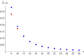
Fig. 1 shows the numerical results for $P_{A},\bar{P}_{A}$ and $P_{A}-\bar{P}_{A}$ for an equal bipartition with $n=2m$ with $n=8$ up to to 30. Notice that the $P_{A}-\bar{P}_{A}$ decreases for increasing values of $n$, that confirms the accuracy of the approximation of $\rho_{A}$ by $\bar{\rho}_{A}$.

Figure 1: Purity as a measure of entanglement for the Prime state. Left: Purity for $n=8-30$ computed with the exact density matrix $\rho_{A}$ in Eq. (40) (red on line) and the density matrix $\bar{\rho}_{A}$ in Eq. (52) (blue of line). Right: difference $\bar{P}_{A}-P_{A}$.

III.5 Numerical results for the von Neumann entanglement entropy

The von Neumann entropy provides a figure of merit for quantifying entanglement which has extensive used in other quantum contexts, as in the fields of Condensed Matter or of black hole physics. Quite remarkably, it has proven to be an adequate instrument to analyze the entanglement of the ground state of spin Hamiltonians and it is used to detect and classify quantum phase transitions. In such situations, the scaling of the von Neumann entropy with the size of the system obeys the so-called ”area law”. A similar behavior is encountered in particle physics and in the holographic description of black holes. Furthermore, the von Neumann entropy has an operational meaning. It describes the number of singlets that can be distilled from a given state as the available copies of that state go to infinity. It is, thus, natural to investigate how much entropy of entanglement is carried by the Prime state.

From a technical point of view, the von Neumann entropy is difficult to calculate. The fact that we need to compute a logarithm of the reduced density matrix makes an analytical approach not at all trivial. Here, we shall present numerical results on this entanglement entropy for the Prime state up to $n=30$. To be precise, we consider the Prime state at different values of $n$, $n=4,\ldots,30$ and shall take its bi-partitions. Given a bi-partition, we compute the reduced density matrix for such a partition and then compute its associated von Neumann entropy.

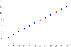
Our main numerical result on the von Neumann entropy of the Prime state $|\vbox{\hbox{\upright\hbox to0.0pt{I\hss}\kern 1.5ptP}}_{n}\rangle$ is the scaling it shows as $n$ increases. This is shown in Fig. 2, where we plot the actual results and a best fit to a line, $S(n)=\alpha n/2+\beta$. We find that the slope of this best fit is $\alpha=.886(1)$. Note that the absolute maximal entanglement would correspond to the maximum possible slope $\alpha=1$. It follows that the Prime state seems to present maximal scaling, which is proportional to $n$, with a coefficient which is less than 1. As in the case of the Renyi -2 entropy, we interpret this result as being due to the existence of correlations in the primes. In section III C we obtain an analytic estimate of the constant $\alpha$, based on the entanglement spectrum of the density matrix $\bar{\rho}_{A}$.

Let us emphasize that it is expected that the Prime state should carry very large entanglement. If this were not the case, we could apply standard efficient techniques like Matrix Product States to handle its properties (for a review see CV ). The fact that the Prime state is so highly entangled is just preventing the applicability of some powerful tools which are useful on standard physical systems. To have a better understanding of this point, we compare in Table 1 the known scaling of entanglement in different systems.

Figure 2: Von Neumann entropy as a measure of entanglement for the Prime state. Left: Entanglement entropy for $n=8-30$ computed with the exact density matrix $\rho_{A}$ (red on line) and the approximation Eq. (52) (blue of line). Right: differences $S_{A}-\bar{S}_{A}$.

infinite non-critical spin chains	$S\sim\frac{c}{6}\log\xi$, $\xi$ correlation length
critical spin chains, block of size $L$	$S\sim\frac{c}{3}\log\L$
2D systems, square of size $L$	$S\sim L$
Prime state of $n$-bits	$S\sim\alpha n/2$, $\alpha\sim.886(1)$
maximally entangled states	$S\sim n/2$

Table 1: Scaling of von Neumann entropy for different quantum systems. In the case of spin chains, $c$ is the central charge of the underlying CFT.

Figure 3: Histogram showing the entanglement entropy of 1000 random partitions of the Prime state with $n=20$ quits (the abscissa corresponds to the entropy). The right-most point, with largest entropy, corresponds to the natural partition.

The interpretations of large classical and quantum entropies are related to surprise. We may rephrase the maximal scaling of entanglement in the following way. Suppose that we know the first $n/2$ digits of a prime. Then, knowing the second $n/2$ digits provides a classical surprise which is almost maximal. Then, let us think of the quantum superposition of primes. The correlation between all the first $n/2$ digits and the rest is almost maximal. We cannot disentangle the first and second part of the register.

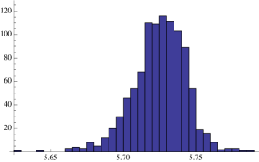
Let us now turn to the study of different partitions of the Prime state. We consider random bi-partitions of the Prime state which need not be sequential, that is the party $A$ is made out of $n/2$ qubits, randomly chosen out of the $n$ available ones. Fig.3 shows the von Neumann entropy for large sets of bi-partitions of $n=20$ qubits. It is remarkable that the maximum entropy is found for the natural partition of the Prime state. This fact is systematically observed for all values of $n$ we have been able to checked. It is unclear if this is a fundamental fact about the distribution of primes. A similar result is obtained if purity is analyzed. Again the natural partition shows more entanglement than any other one.

III.6 Majorization of twin primes by primes

Twin primes form a series which has been thoroughly analyzed in Number Theory. It was shown in section II that a Twin Prime quantum state can be constructed using the same technology as for the Prime state. We may as well ask whether the Twin Prime state is more or less entangled than the Prime state. The answer to this question is shown in Table 2.

n	S(prime)	S(twin prime)
10	3.1900	3.3450
12	4.0220	4.5221
14	4.8993	5.4438
16	5.7872	6.4812
18	6.6748	7.4908
20	7.5574	8.4834
22	8.4428	9.4796
24	9.3301	10.4729
26	10.2159	11.4644
28	11.1018	12.4551
30	11.9876

Table 2: Comparison between the von Neumann entropy for the Prime state and the Twin Prime state. The Twin Prime state carries more correlation than primes.

The Twin Prime state appears to carry more entanglement than the Prime state. This is somewhat reasonable. Twin primes are more scarce than primes, $N/\log^{2}N$ as compare to $N/\log N$. Yet, the maximum of entropy requires only $N^{1/2}$ superpositions, which is far less than the actual number of twin primes. It seems that the more dilute twin primes are then enough to carry more surprise in their appearances.

We may now wonder whether the probability density described by the entanglement spectrum of the Prime state, $\lambda_{i}^{(p)}$ with $i=1,\ldots,2^{n/2}$, is strongly ordered with respect to the equivalent entanglement spectrum in the Twin Prime state, $\lambda_{i}^{(p,p+2)}$ with $i=1,\ldots,2^{n/2}$. This is indeed the case. It is easy to verify that for large $n$ the following $2^{n/2}$ relations hold

$$\lambda^{(p)}_{1} > \lambda^{(p,p+2)}_{1}$$

$$\lambda^{(p)}_{1}+\lambda^{(p)}_{2} > \lambda^{(p,p+2)_{1}}+\lambda^{(p,p+2)}_{2}$$

$$\ldots \ldots$$

$$\lambda^{(p)}_{1}+\ldots+\lambda^{(p)}_{2^{n/2}} > \lambda^{(p,p+2)}_{1}+\ldots+\lambda^{(p,p+2)}_{2^{n/2}}.$$ (60)

Thus, the Prime state spectrum majorizes the Twin Prime spectrum

$$\vec{\lambda}^{(p,p+2)}\prec\vec{\lambda}^{(p)}.$$ (61)

This is remarkable sense of order usually named majorization. From an operational point of view, majorization is stated about the possibility of connecting quantum states using Local Operations and Classical Communication. In our case, the general theorems mean that if two parties $A$ and $B$ can carry unitaries on their local part of a quantum state and can also communicate classically, then the Twin Prime state can be transformed into the Prime state. This is a consequence of the majorization relations that they obey.

We have further explored whether there are majorization relations for triples of primes, those with the form $(p,p+2,p+6)$ or $(p,p+4,p+6)$. We have analyzed the first of these cases and found again a relation of majorization

$$\vec{\lambda}^{(p,p+2,p+6)}\prec\vec{\lambda}^{(p,p+2)}\prec\vec{\lambda}^{(p)}.$$ (62)

if $n$ is sufficiently large. At small $n$ the fluctuations of primes do spoil the majorization relation, but this transient situation goes away monotonically as $n$ grows.

It is tantalizing to conjecture that an infinite series of majorization relations, that is a deep sense of ordering, settles in the set of subseries of primes. The more sparse sub-series of primes will typically majorize the denser ones.

IV Analytical approximation to the entanglement spectrum

The different measures of entanglement we have computed for the Prime state are ultimately based on the precise distribution of eigenvalues of its Schmidt decomposition. As a matter of fact, the spacing and degeneracy of these eigenvalues contain deep information on the quantum correlations of the state. We shall shortly show that the detailed analysis of this spectrum of eigenvalues hints at an analytical approximation to the entanglement properties of the Prime state, that we shall later exploit.

The entanglement spectrum of the density matrix $\rho_{A}$ is defined in terms of its eigenvalues $\lambda_{i}$ as follows

$$\varepsilon_{i}=-\log\lambda_{i},\qquad i=1,\ldots,2^{m},$$ (63)

and they are the eigenvalues of the entanglement Hamiltonian $H_{E}$ defined as $\rho_{A}=e^{-H_{E}}$. The states with lowest entanglement energy are therefore those with highest values of $\lambda_{i}$. This definition was introduced in the context of the Fractional Quantum Hall effect, where the low energy entanglement spectrum of the ground state, at several filling fractions, was shown to correspond to the Conformal Field Theory that describes the physical edge excitations of the system LH . This result suggests a bulk-edge correspondence in strongly correlated many-body systems that is reminiscent to the holographic principle in String Theory.

Figure 4: Entanglement spectrum for $n=30$. It is plotted the lowest 89 states. Left: EE’s of $\rho_{A}$ (red on line). Right: EE’s of $\bar{\rho}_{A}$ (blue on line). Right: Superposition of EE of $\rho_{A}$ and $\bar{\rho}_{A}$.

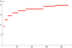
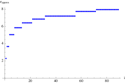
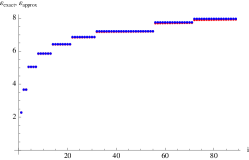
We have computed the entanglement spectrum of the Prime state using the exact density matrix $\rho_{A}$ of Eq. (40) and the approximation $\bar{\rho}_{A}$ of Eq. (48). Fig. 4 shows the lowest 89 states for $n=30$ qubits with a bipartition $m=n/2=15$. We first notice that the exact and the approximated values of $\varepsilon_{i}$ agree rather well, specially in the low energy part, and that the agreement improves increasing the number of qubits $n$. The more interesting feature is the appearance of nearly degenerated energy eigenstates, particularly visible for $\bar{\rho}_{A}$. We shall now obtain an analytical approximation to these eigenvalues and their degeneracies.

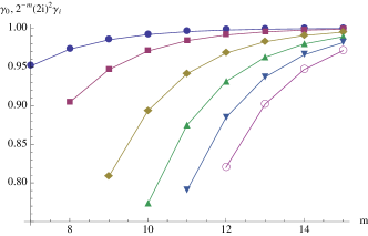
Note that the relation in Eq. (52) implies that the degeneracy in the entanglement spectrum must be originated in the eigenvalues $\gamma_{i}$ of the matrix ${\bf C}$. In our case, we work with a finite amount of primes, so that we have ${\bf C}_{m}$, where $m=n/2$, that approaches ${\bf C}$ as the number of qubits in the Prime state goes to infinity. The lowest eigenvalue, $\gamma_{0}$, is unique but the positive higher eigenvalues $\gamma_{i}\;(i\geq 1)$ have a degeneracy $2i$ and are given by

$$\gamma_{0}=2^{m},\qquad\gamma_{i}=\frac{2^{m}}{(2i)^{2}}\quad(i=1,2,\dots,k_{m}),$$ (64)

where the value of $k_{m}$ associated to the largest eigenvalue will be computed shortly. Fig. 5 shows a numerical check of this relation as a function of the number of qubits $m$ of the block $A$. Eqs.(52) and (64), imply the following approximation for the eigenvalues of the density matrix $\bar{\rho}_{A}$,

$$\lambda_{0}=2^{1-m}(1+\ell_{N}2^{m}),\qquad\lambda_{i}=2^{1-m}\left(1+\ell_{N}\frac{2^{m}}{(2i)^{2}}\right)\quad(i=1,2,\dots,k_{m}),$$ (65)

where $\ell_{N}$ is given by eq.(47) with $n=2m$. To fix the value of $k_{m}$ we shall impose the normalization of the density matrix $\bar{\rho}_{A}$, that is

Figure 5: Verification of the relation (64) for the eigenvalues of the matrix ${\bf C}_{m}$ as a function of $m=7,\ldots,15$. From top to bottom we plot $\gamma_{0},\gamma_{1},\dots,\gamma_{5}$. Notice that the relation becomes exact in the limit $m\rightarrow\infty$.

$$\lambda_{0}+\sum_{i=1}^{k_{m}}2i\,\lambda_{i}=1,$$ (66)

which for large values of $m$ yields

$$k_{m}\simeq\kappa_{0}\,2^{m/2}(1-\beta/m),\quad\kappa_{0}=\sqrt{\frac{3}{8}},\quad\kappa_{1}=1.0035..$$ (67)

The matrix ${\bf C}_{m}$ is traceless, so there are negative eigenvalues whose sum compensates the sum of the positive eigenvalues in Eq. (64). The magnitude of the former ones is small which implies that the corresponding eigenvalues of $\bar{\rho}_{A}$ will also be small. We shall show below that the positive eigenvalues (64) dominate the traces of the powers of the matrix ${\bf C}_{m}$, and consequently the Renyi and von Neumann entropies. Let us first compute

$${\rm Tr}\,{\bf C}_{m}^{s} \approx \gamma_{0}^{s}+\sum_{i=1}^{k_{m}}2i\,\gamma_{i}^{s}=2^{ms}\left(1+\sum_{i=1}^{k_{m}}\frac{1}{(2i)^{2s-1}}\right)\xrightarrow{\scriptscriptstyle m\to\infty}2^{ms}\left(1+\frac{\zeta(2s-1)}{2^{2s-1}}\right),\quad s>1.$$ (68)

where we took the limit $m\rightarrow\infty$ in the sum, which gives rise to the Riemann zeta function $\zeta(2s-1)$. Notice that the series diverges if $s\rightarrow 1$ because we have dropped the negative eigenvalues. For $s=2$, one obtains

$${\rm Tr}\,{\bf C}_{m}^{2}\xrightarrow{\scriptscriptstyle m\to\infty}2^{2m}\left(1+\frac{\zeta(3)}{8}\right)=2^{2m}\times 1.15026..$$ (69)

which agrees to order $10^{-4}$ with the exact asymptotic expression of Eq. (57) derived in Appendix A3

$${\rm Tr}\,{\bf C}_{m}^{2}\xrightarrow{\scriptscriptstyle m\to\infty}2^{2m}\prod_{p>2}\left(1+\frac{1}{(p-1)^{3}}\right)=2^{2m}\times 1.15048...$$ (70)

Based on this numerical result we conjecture the following asymptotic formula for any $s\geq 2$,

$${\rm Tr}\,{\bf C}_{m}^{s}\xrightarrow{\scriptscriptstyle m\to\infty}2^{ms}\prod_{p>2}\left(1+\frac{1}{(p-1)^{2s-1}}\right).$$ (71)

The difference between (71) and (68) is

$$\prod_{p>2}\left(1+\frac{1}{(p-1)^{2s-1}}\right)=\left(1+\frac{\zeta(2s-1)}{2^{2s-1}}\right)+\frac{1}{12^{2s-1}}-\frac{1}{14^{2s-1}}+\dots,$$ (72)

that for $s=3$ explains the proximity of the constants in Eqs. (69) and (70). Let us note that the zeta function term approximates exponentially well the infinite product over primes. In table 3 we compare Eqs. (71) and (68) with the numerical results obtained by extrapolating ${\rm Tr}\,{\bf C}_{m}^{s}$ for $m=9,\dots,15$.

$s$	$1+\frac{\zeta(2s-1)}{2^{2s-1}}$	$\prod_{p>2}(1+(p-1)^{1-2s})$	$\lim_{m\rightarrow\infty}2^{-ms}{\rm Tr}\,{\bf C}_{d}^{2}$
2	1.15025711	1.15048076	1.15048162
3	1.03240399	1.03240618	1.03241334
4	1.00787772	1.00787774	1.00788749
5	1.00195704	1.00195704	1.00197171

Table 3: Comparison of $\lim_{m\rightarrow\infty}2^{-ms}{\rm Tr}\,{\bf C}_{m}^{2}$ computed with Eqs. (68), (71) and the numerical values obtained with the fit formula $a_{0}+2^{-m}\sum_{j=0}^{3}a_{j}\,m^{j}$ with $m=9,\dots,15$.

To calculate the entanglement entropy we use Eq.(65) and replace the sum over the eigenvalues by an integral

$$S_{A} \approx -(\lambda_{0}\log\lambda_{0}+\sum_{i=1}^{k_{m}}2i\lambda_{i}\log\lambda_{i})$$

$$\approx -\int_{1}^{k_{m}}dx\,x\;2^{2-m}\left(1+\frac{\ell_{N}2^{m-2}}{x^{2}}\right)\log\left[2^{1-m}\left(1+\frac{\ell_{N}2^{m-2}}{x^{2}}\right)\right].$$

Then computing the two leading terms in the asymptotic limit $m\rightarrow\infty$ we obtain an analytical approximation to the von Neumann entropy

$$S_{A}\xrightarrow{\scriptscriptstyle m\to\infty}\frac{7}{8}m+\frac{1}{4}\log m+{\rm cte},\qquad m\rightarrow\infty.$$ (74)

For other values of the parameter $\kappa_{0}$, giving $k_{m}$ in Eq.(67), the constant of the linear term in (IV) is given by $(1+16\kappa_{0}^{2})/8$, that becomes $7/8=0.875$ for $\kappa_{0}=\sqrt{3/8}$. Observe that the latter constant is close to the numerical value $0.886(1)$ obtained from the spectrum of the density matrix $\rho_{A}$ up to sizes $m=15\;(n=30)$ given in Table 1.

V Novel number theoretical states

The prime state can be generalized to many other states associated to arithmetic functions. Consider for example the Moebius function $\mu(n)$. Factorizing $n$ into products of primes, $n=p_{1}^{r_{1}}\dots p_{s}^{r_{s}}$, then $\mu(n)=0$ if $n$ contains a prime to a power greater than one, $\exists\;i,r_{i}>1$, and if $n$ is the product of $s$ distinct primes, $r_{i}=1,\;\forall i$, then $\mu(n)=(-1)^{s}$,

$$n=p_{1}^{r_{1}}\dots p_{s}^{r_{s}},\quad\mu(n)=\left\{\begin{array}[]{cc}(-1)^{r_{1}+\dots+r_{s}}&{\rm if}\;r_{1}=\dots=r_{s}=1,\\ 1&n=1,\\ 0&{\rm else}\\ \end{array}\right.\ .$$ (75)

The Moebius state shall be defined as

$$|\mu_{n}\rangle=\frac{1}{\sqrt{C_{\mu,n}}}\sum_{a<2^{n}}\mu(a)\,|a\rangle,\quad C_{\mu,n}=\sum_{a<2^{n}}|\mu(a)|,$$ (76)

where $C_{\mu,n}$ ensures that $\langle\mu_{n}|\mu_{n}\rangle=1$. This constant can be estimated using the quantum counting protocol employed to compute $\pi(2^{N})$ LS . The similarity between the prime state of Eq. (1) and the Moebius state of Eq. (76) is made manifest writing Eq. (1) in terms of the characteristic function $\chi_{\pi}$

$$|\vbox{\hbox{\upright\hbox to0.0pt{I\hss}\kern 1.5ptP}}_{n}\rangle=\frac{1}{\sqrt{\pi(2^{n})}}\sum_{a<2^{n}}\chi_{\pi}(a)|a\rangle,\quad\pi(2^{n})=\sum_{a<2^{n}}\chi_{\pi}(a).$$ (77)

The Moebius state encodes quantum mechanically the information contained in $\mu(n)$. As in the case of the Prime state one can extract part of this information performing measurements. An example of this method is provided by the Mertens function Apostol

$$M(n)=\sum_{a\leq n}\mu(a),\quad n=1,2,\dots$$ (78)

$M(2^{n})$ can be measured projecting the Moebius state into the Hadamard state of $n$ qubits

$$|H_{n}\rangle=\frac{1}{2^{n/2}}\sum_{a<2^{n}}|a\rangle,$$ (79)

that gives

$$\langle H_{n}|\mu_{n}\rangle=\frac{1}{2^{n/2}C_{n}^{1/2}}M(2^{n}).$$ (80)

The constant $C_{\mu,n}$ is known from quantum counting so $M(2^{n})$ can be determined within some error inherent to quantum measurements. The Riemann hypothesis implies that $|M(x)|=O(x^{\frac{1}{2}+\epsilon}),\,\forall\epsilon>0$ Ti , so one could try to verify its validity, as was explained in section II C using the Prime state.

In previous sections we have shown that the Prime state contains a high degree of entanglement that is intimately connected to the pairwise correlations between the prime numbers. The Moebius state, and most of the states built using arithmetic functions, are expected to be entangled. One may ask what is the relation between the arithmetic functions and the measurements of entanglement of the corresponding states? We shall not consider here this problem, and only make some suggestions.

The arithmetic quantum states of the form in Eqs. (1) and (76) can be generalized to the Dirichlet series,

$$f(s)=\sum_{n=1}^{\infty}\frac{f(n)}{n^{s}},\qquad\Re\,s>\sigma_{c},$$ (81)

where $f(n)$ is an arithmetic function, and $s=\sigma+it$ a complex variable whose real part $\sigma$ must be bigger than some value $\sigma_{c}$ to ensure the convergence of the series Apostol . An example of Eq. (81) is the Riemann zeta function $\zeta(s)=\sum_{n=1}^{\infty}1/n^{s}$, where $\sigma_{c}=1$. We can associate to $f(s)$ the Dirichlet state

$$|f(s)_{n}\rangle=\frac{1}{\sqrt{C_{f,n}(\sigma)}}\sum_{a<2^{n}}\frac{f(a)}{a^{s}}\,|a\rangle,\quad C_{f,n}(\sigma)=\sum_{a<2^{n}}\frac{|f_{n}(a)|^{2}}{a^{2\sigma}},\quad s=\sigma+it.$$ (82)

In the limit $n\rightarrow\infty$, the normalization constant $C_{f,n}(\sigma)$, becomes a Dirichlet series whose radius of convergence will be bigger than $\sigma_{c}$. Consider again the case of $\zeta(s)$ where

$$\lim_{n\rightarrow\infty}C_{\zeta,n}(\sigma)=\sum_{n=1}^{\infty}\frac{1}{n^{2\sigma}}=\zeta(2\sigma),\qquad\sigma>\frac{1}{2},$$ (83)

that allows us to define a normalized state associated to $\zeta(s)$, including the critical region $\frac{1}{2}<\sigma\leq 1$, where Eq. (81) diverges and $\zeta(s)$ is defined by analytic extension. The Riemann state can then be defined as

$$|\zeta(s)\rangle=\frac{1}{\sqrt{\zeta(2\sigma)}}\sum_{n=1}^{\infty}\frac{1}{n^{s}}\,|n\rangle,\quad\sigma>\frac{1}{2}.$$ (84)

We expect this state, or its finite qubit version in Eq. (82), to exhibit different entanglement properties in the critical region $\frac{1}{2}<\sigma\leq 1$ and in the non-critical one $\sigma>1$, that may in turn be related to the properties of $\zeta(s)$ itself. Similarly, in the limit $n\rightarrow\infty$ we can associate a quantum state to any Dirichlet $L$-function with character $\chi$

$$L_{\chi}(s)=\sum_{n=1}^{\infty}\frac{\chi(n)}{n^{s}}\longrightarrow|L_{\chi}(s)\rangle=\frac{1}{\sqrt{\bar{L}_{\chi}(2\sigma)}}\sum_{n=1}^{\infty}\frac{\chi(n)}{n^{s}}\,|n\rangle,\quad\bar{L}_{\chi}(\sigma)=\sum_{n=1}^{\infty}\frac{|\chi(n)|}{n^{2\sigma}}.$$ (85)

These examples shows that one can assign entanglement properties not only to prime numbers and arithmetic functions, but also to the Riemann and Dirichlet $L$- functions, opening a novel approach to Number Theory using the tools of Quantum Information Theory.

VI Conclusions

Quantum Mechanics offers a completely new approach to Arithmetics, that may be called Quantum Arithmetics. The essential point is the possibility of producing a quantum superposition of series of numbers, that can then be processed and analyzed in parallel. In this paper, we have shown that the series of prime numbers can be assigned a Prime state. This Prime state can be created efficiently and can be exploited to find properties of the series of prime numbers in a way that goes beyond classical computational methods. As a relevant example, we have shown that the Prime state can be used to verify the Riemann Hypothesis in a more efficient way than any existing classical algorithm.

We have shown that the density matrix of the Prime state is characterized, asymptotically, by the Hardy-Littlewood constants that parametrize the pair correlations between prime numbers. This result establish a link between between prime correlations and entanglement of the Prime state. We have also studied the figures of merit of entanglement in this state, such as purity, von Neumann entropy and entanglement spectrum. The main result stays than the Prime state entanglement is almost maximal. As a consequence, it follows the inefficiency of using clever tensor networks algorithms to manipulate it.

Acknowledgements. The authors are grateful to J. I. Cirac, A. Córdoba, S. Iblisdir and J. Keating for helpful comments and to A. Monràs for his help on the computation of entropies. J. I. L. acknowledges financial support from FIS2011-16185, Grup de Recerca Consolidat ICREA-ACADÈMIA, and National Research Foundation & Ministry of Education, Singapore; and G. S. from the grants FIS2012-33642, QUITEMAD and the Severo-Ochoa Program.

Appendix A1: Derivation of $\rho_{A}$

In this section we shall find an explicit expression of the density matrix $\rho_{A}$ in Eq. (28) in terms of number theoretical functions whose asymptotic properties will be presented in Appendix A2. To do so we shall treat separately the blocks corresponding to $m=1$ and $m>1$. If $m=1$, the matrix $\rho_{A}$ is given by LS

$$m=1:\;\rho^{A}_{0,0}=\frac{1}{\pi(N)},\quad\rho^{A}_{1,1}=\frac{\pi(N)-1}{\pi(N)},\quad\rho^{A}_{0,1}=\frac{1}{\pi(N)}.$$ (86)

These equations follow from the observation that all the primes are odd numbers but $p=2$, which implies

$$p=2 \rightarrow \psi_{b,0}=\delta_{b,1},$$ (87)

$$p>2 \rightarrow \psi_{b,1}=\left\{\begin{array}[]{ll}1&{\rm iff}\;\;p=1+2b:{\rm prime},\\ 0&{\rm else}.\\ \end{array}\right..$$ (90)

The numerators of $\rho^{A}_{a,a^{\prime}}$, means that 2 is a prime number ($(a,a^{\prime})=(0,0)$), that there are $\pi(N)-1$ odd prime numbers ($(a,a^{\prime})=(1,1)$) and that $2$ and $3$ are primes ($(a,a^{\prime})=(0,1)$).

Let us next consider the cases where $m>1$. Since $\psi_{a,b}=0$ or 1, $\forall a,b$, one can write the diagonal entries of $\rho_{A}$ as

$$\rho^{A}_{a,a}=\frac{1}{\pi(N)}\sum_{b<2^{m^{\prime}}}\psi_{b,a}.$$ (91)

In this equation the sum gives the number of primes of the form $p=a+2^{m}\,b$ less than $N$, where $a\in[0,2^{m}-1]$ is fixed and $b$ varies in the interval $[0,2^{m^{\prime}}-1]$. If $a$ is even so is $p$, because $2^{m}b$ is always even or zero. Hence $p$ is equal to 2, and then $a=2$ and $b=0$, which yields

$$m>1,\;a:{\rm even}\rightarrow\psi_{b,a}=\delta_{b,0}\delta_{a,2}.$$ (92)

Note that the condition $m>1$ is required to allow $a$ to take the value 2. Using Eq.(92) into Eq. (91) one finds

$$m>1,\;a:{\rm even}\rightarrow\rho^{A}_{a,a}=\frac{\delta_{a,2}}{\pi(N)}.$$ (93)

If $a$ is odd, the primes $p=a+2^{m}b$, form an arithmetic progression $cn+d\,(n=0,1,\dots)$ where $c=2^{m}$ and $d=a$ are coprime numbers, that its with no common divisor. Using the standard notation $\pi_{c,d}(x)$ for the number of primes less or equal to $x$ contained in the arithmetic progression $cn+d$, where $c$ and $d$ coprime numbers, we can then write

$$m>1,\;a:{\rm odd}\rightarrow\rho^{A}_{a,a}=\frac{\pi_{M,a}(N)}{\pi(N)},\quad M=2^{m}.$$ (94)

Let us next consider the off-diagonal terms $\rho^{A}_{a,a^{\prime}}$. If $a\neq a^{\prime}$ are both even, one can use Eq.(92) to derive

$$m>1,\;a\neq a^{\prime}:{\rm even}\rightarrow\rho^{A}_{a,a^{\prime}}=0.$$ (95)

If $a$ is even and $a^{\prime}$ odd using again Eq.(92) one finds

$$m>1,\;a:{\rm even},\;a^{\prime}:{\rm odd}\rightarrow\sum_{b<2^{m^{\prime}}}\psi_{b,a}\,\psi_{b,a^{\prime}}=\delta_{a,2}\,\psi_{0,a^{\prime}}.$$ (96)

Eq. (22) implies that $\psi_{0,a}=1$ if $a$ is a prime and $\psi_{0,a}=0$ if it is not. So $\psi_{0,a}$ is equal to the characteristic function of prime numbers $\chi_{\pi}(a)$. We have then derived

$$m>1,\;a:{\rm even},\;a^{\prime}:{\rm odd}\rightarrow\rho^{A}_{a,a^{\prime}}=\frac{\delta_{a,2}\,\chi_{\pi}(a^{\prime})}{\pi(N)}.$$ (97)

Finally, in order to compute $\rho^{A}_{a,a^{\prime}}$, when $a\neq a^{\prime}$ are both odd, we shall use the counting function $\pi_{a;b,b^{\prime}}(x)$ defined by Eq.(38). The sum in the expression Eq. (28) for $\rho^{A}_{a,a^{\prime}}$, when $a<a^{\prime}$ are both odd, is the number of pairs of odd primes of the form $(p,p^{\prime})=(a+2^{m}b,a^{\prime}+2^{m}b)$, with $p\leq N$ and $p^{\prime}\leq N$. This is just the counting function $\pi_{a;b,b^{\prime}}(x)$ with $(x,a,b,b^{\prime})\rightarrow(N,M,a,a^{\prime})$, hence

$$m>1,\;a:{\rm odd},\;a^{\prime}:{\rm odd}\rightarrow\rho^{A}_{a,a^{\prime}}=\frac{\pi_{M;a,a^{\prime}}(N)}{\pi(N)}.$$ (98)

Collecting the previous results in a block form (even, odd) one finds

$$\rho_{A}=\frac{1}{\pi(N)}\left(\begin{array}[]{cc}\delta_{a,2}\delta_{a^{\prime},2}&\delta_{a,2}\,\chi_{\pi}(a^{\prime})\\ \delta_{a^{\prime},2}\,\chi_{\pi}(a)&\delta_{a,a^{\prime}}\pi_{M,a}(N)+(1-\delta_{a,a^{\prime}})\pi_{M;a,a^{\prime}}(N)\\ \end{array}\right).$$ (99)

As an example, let us choose a system with $n=6$ qubits. The prime state in Eq. (1) contains $\pi(2^{6})=18$ terms corresponding to all the primes less that $N=64$. We split the system into two blocks with $m=m^{\prime}=3$ qubits each. The binary representation of the primes yields the function $\psi_{b,a}$ of Eq.(22) which we write in matrix form as

$$\psi=\left(\begin{array}[]{cccc|cccc}0&1&0&0&0&1&1&1\\ 0&0&0&0&1&1&0&1\\ 0&0&0&0&0&0&1&0\\ 0&0&0&0&0&0&1&0\\ \hline\cr 0&0&0&0&0&1&1&0\\ 0&0&0&0&0&0&1&1\\ 0&0&0&0&1&1&0&1\\ 0&0&0&0&0&1&1&0\\ \end{array}\right)\leftrightarrow\left(\begin{array}[]{cccc|cccc}0&2&0&0&0&3&5&7\\ 0&0&0&0&17&19&0&23\\ 0&0&0&0&0&0&37&0\\ 0&0&0&0&0&0&53&0\\ \hline\cr 0&0&0&0&0&11&13&0\\ 0&0&0&0&0&0&29&31\\ 0&0&0&0&41&43&0&47\\ 0&0&0&0&0&59&61&0\\ \end{array}\right)$$ (100)

where the rows and columns corresponds to the indices $b$ and $a$ respectively which are ordered in the even-odd sequence: $(0,2,4,6,1,3,5,7)$. The matrix on the RHS gives the associated prime numbers, for example $\psi_{4,5}=1$ corresponds to $p=5+2^{3}\times 4=37$. The density matrix $\rho_{A}$ can be readily computed as the product

$$\rho_{A}=\frac{1}{\pi(2^{6})}\psi^{\dagger}\,\psi=\frac{1}{18}\left(\begin{array}[]{cccc|cccc}0&0&0&0&0&0&0&0\\ 0&1&0&0&0&1&1&1\\ 0&0&0&0&0&0&0&0\\ 0&0&0&0&0&0&0&0\\ \hline\cr 0&0&0&0&2&2&0&2\\ 0&1&0&0&2&5&3&3\\ 0&1&0&0&0&3&6&2\\ 0&1&0&0&2&3&2&4\\ \end{array}\right).$$ (101)

Comparing this matrix with the expression in Eq. (99) one verifies the even-even, even-odd and odd-even blocks, the latter ones following from the identities $\chi_{\rm prime}(i)=1$ for $i=3,5,7$. The diagonal entries of the odd-odd block are given by the number of primes in the arithmetic progressions $8k+a$ with $a=1,3,5,7$,

$$\pi_{8,1}(64)=2 : \left\{17,41\right\}$$ (102)

$$\pi_{8,3}(64)=5 : \left\{3,11,19,43,59\right\}$$

$$\pi_{8,5}(64)=6 : \left\{5,13,29,37,53,61\right\}$$

$$\pi_{8,7}(64)=4 : \left\{7,23,31,47\right\}$$

Similarly, the off-diagonal entries of the odd-odd block counts the number of pairs in the associated arithmetic progressions:

$$\pi_{8;1,3}(64)=2 : \left\{(17,19),(41,43)\right\}$$ (103)

$$\pi_{8;1,5}(64)=0 : \left\{\right\}$$

$$\pi_{8;1,7}(64)=2 : \left\{(17,23),(41,47)\right\}$$

$$\pi_{8;3,5}(64)=3 : \left\{(3,5),(11,13),(59,61)\right\}$$

$$\pi_{8;3,7}(64)=3 : \left\{(3,7),(19,23),(43,47)\right\}$$

$$\pi_{8;5,7}(64)=2 : \left\{(5,7),(29,31)\right\}$$

Notice that $17$ and $13$ belong to the series $1\,{\rm mod}\,8$ and $5\,{\rm mod}\,8$ respectively, and that $17=8\times 2+1$ and $13=8\times 1+5$. Hence they do not satisfy the definition in Eq. (38), and therefore do not contribute to $\pi_{8;1,5}(64)$ which is actually zero.

Appendix A2: Asymptotic limit of prime counting functions

In this appendix we present numerical results concerning the asymptotic behavior of several prime number functions that appear in the main text. Some of the results are well known but others are new, as far as we know.

VI.1 The prime counting function $\pi(N)$

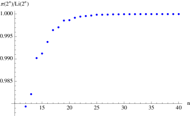
The PNT given in Eq. (4) is stated more precisely as the limit

$$\lim_{N\rightarrow\infty}\frac{\pi(N)}{Li(N)}=1.$$ (104)

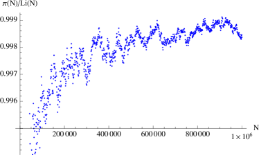
Fig. 6 shows the convergence of the ratio $\pi(N)/Li(N)$ for two examples. In the case where $N=2^{n}$ the fluctuations are not as visible as in the first case, but they lie within the limits imposed by the Riemann hypothesis, that are of order $N^{-1/2}\log^{2}N$ as shown in Eq. (5). From Fig.(6) one would be tempted to conjecture that $\pi(N)<Li(N)$, for all $N$. However, Littlewood showed in 1914 that the difference $\pi(N)-Li(N)$ changes infinitely often. It is not known the lowest value of $N$, for which $\pi(N)>Li(N)$. Skewes gave a first estimate in terms of the googolian number $10^{10^{10^{34}}}$, known as the Skewes number, but this upper bound value has been reduced to a modest $e^{729}\sim 3.98\times 10^{316}$.

Figure 6: Numerical verification of the PNT in Eq. (104). Left: $N=10^{3}-10^{6}$ in steps of $10^{3}$. Right: $N=2^{n}$ for $n=10-40$.

VI.2 The prime counting function for arithmetic series $\pi_{a,b}(N)$

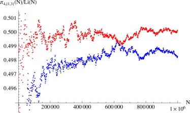
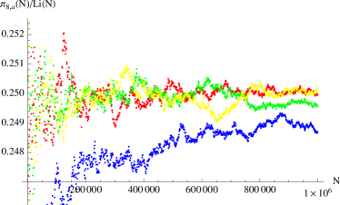
The PNT for arithmetic progressions, Eq.(33), amounts to

$$\lim_{N\rightarrow\infty}\frac{\pi_{a,b}(N)}{Li(N)}=\frac{1}{\phi(a)},\qquad gcd(a,b)=1,$$ (105)

and is illustrated in Fig. 7 in the cases $\pi_{4,b}(N)$ and $\pi_{8,b}(N)$. Notice that $\pi_{4,3}(N)-\pi_{4,1}(N)$ is mostly positive. This difference is known as the Chebyshev bias and changes infinitely often. Fig. 7 shows one crossing. Similar pattern occurs for $\pi_{8,b}(N)$.

Figure 7: Left: $\pi_{4,b}(N)$ for $b=1$ (blue color on line) and $b=3$ (red color on line). Right: $\pi_{8,b}(N)$ for $b=1$ (blue), $b=3$ (red), $b=5$ (green) and $b=7$ (yellow). The curves converge towards $1/\phi(a)=1/2$ and $1/4$, respectively, in agreement with Eq.(105)

VI.3 The prime correlation function $\pi_{2}(k,N)$

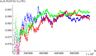
The Hardy-Littlewood conjecture of Eq. (35) reads

$$\lim_{N\rightarrow\infty}\frac{\pi_{2}(k,N)}{Li_{2}(N)}=C(k),$$ (106)

where $C(k)$ is defined in Eq.(36). Fig. 8 depicts this limit for $k=2,4,6$, where $C(k)$ takes the following values

$$C(2)=1.32032..,\quad C(4)=C(2),\quad C(6)=2C(2).$$ (107)

Figure 8: Illustration of Eq.(106) for $k=2,4,6$.

VI.4 The arithmetic correlation function $\pi_{M,a,a^{\prime}}(N)$

Eq. (39) means

$$\lim_{N\rightarrow\infty}\frac{\pi_{M;a,a^{\prime}}(N)}{Li_{2}(N)}=\frac{C(|a-a^{\prime}|)}{\phi(M)}$$ (108)

and it is illustrated in Fig. 9 for $M=8$.

Figure 9: Illustration of Eq.(108) for $M=8$. Left: $(a,a^{\prime})=(1,3),(3,5),(5,7)$ (color on line: blue, red, green). Center: $(a,a^{\prime})=(1,5),(3,7)$ (color on line: blue, red). Right: (a, a’) = (1,7) (color on line: blue). Note that $C(2)=C(4)=C(6)/2$ and $\phi(8)=4$, which explains the asymptotic values of the abcissas.

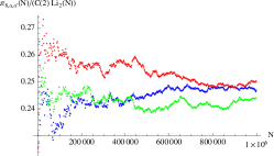
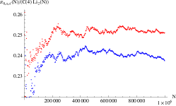
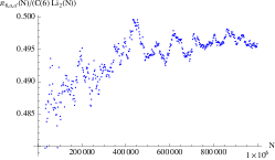
Appendix A3: The Hardy-Littlewood constants $C(k)$

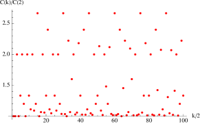
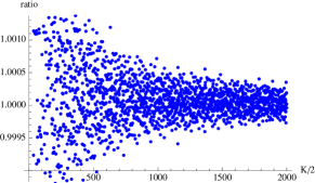
The constants $C(k)$ that appear in the Hardy-Littlewood conjecture in Eq. (36) vary irregularly with $k$. The behavior is shown in Fig.10-left. However, the sum of $C(k)$ satisfies an asymptotic formula obtained by Keating K93 ; BK99 (see in Fig.10-right),

$$\sum_{k=1}^{K}C(k)\sim K-\frac{1}{2}\log K,\qquad K>>1,$$ (109)

which implies the average asymptotic behavior

$$\langle C(k)\rangle\sim 1-\frac{1}{2|k|},\qquad k\gg 1.$$ (110)

Figure 10: Left: $C(k)/C(2)$ for $k=2,4,\dots,200$. Right: ratio = $\sum_{k=1}^{K}C(k)/(K-\frac{1}{2}\log K)$ for $K$ up to 4000.

The approximation in Eq. (110) played a crucial role in the derivation of the statistics of the Riemann zeros that is described by the Gaussian Unitary Ensemble (GUE), as conjectured by Montgomery in the 70’s and confirmed numerically by Odlyzko in the 80’s. In our study of the entanglement of the Prime state, instead of Eq.(109) we need the asymptotic behavior of ${\rm Tr}\,{\bf C}_{m}^{\alpha}$ for $\alpha=2,3,\dots$. In the case $\alpha=2$, that is ${\rm Tr}\,\bar{\rho}_{A}^{2}$, we need the asymptotic behavior of $\sum_{a,a^{\prime}}^{K}C(|a-a^{\prime}|)^{2}$, that will be computed below using the probabilistic methods that lead to Eq. (109). To do so, we shall first review the probabilistic properties of the primes and the division of integers by primes (we follow closely reference K93 ).

VI.5 Asymptotic behaviour of $\sum_{k=1}^{K}C(k)$

The PNT (4) implies that the probability $P(n)$ that $n$ is a prime behaves as

$$P(n)\sim\frac{1}{\log n},\qquad n\rightarrow\infty.$$ (111)

The Hardy-Littlewood conjecture of Eq. (35) means that the probability that both $n$ and $n-m$ are primes is, in the limit $n\rightarrow\infty$,

$$P(n,n-m)\sim P^{2}(n)\,\alpha(m),\qquad n\rightarrow\infty.$$ (112)

where $\alpha(m)$ coincides with $C(m)$ (in this appendix we use the notation of reference K93 ). The probabilistic concepts can be also applied to divisibility of integers. For example, of the positive integers a fraction $1/p$ are divisible by a prime. Hence, for a large integer $n$ the probability that a prime $p$ divides $n$ is given by $1/p$. Similarly, the probability that an integer $n$ is divided by $p$ (i.e. $p|n$), but not by $p^{2}$ (i.e. $p^{2}{\not{|}}n$) is $1/p-1/p^{2}=(p-1)/p^{2}$. The fundamental theorem of Arithmetics imply that division by different primes are independent operations , so from the probabilistic viewpoint the primes are statistically independent variables. Applying these probabilistic techniques one can derive $\alpha(m)$,

$$\alpha(m)=\alpha\prod_{p>2,\,p|m}\left(1+\frac{1}{p-2}\right)\;(m:{\rm even}),\qquad\alpha(m)=0\;(m:{\rm odd}),$$ (113)

where $\alpha/2$ is the twin prime constant

$$\alpha=2\prod_{p>2}\frac{p(p-2)}{(p-1)^{2}}=1.3203...$$ (114)

Let us now factorize $m$ into primes

$$m=2^{b_{0}}p_{1}^{a_{1}}\dots p_{s}^{a_{s}}\quad(p_{i}>2,a_{i}\geq 1,b_{0}\geq 1),$$ (115)

that yields

$$\alpha(m) = \alpha\left(1+\frac{1}{p_{1}-2}\right)\dots\left(1+\frac{1}{p_{s}-2}\right)$$

$$= \alpha\left(1+\sum_{1\leq i\leq s}\frac{1}{p_{i}-2}+\sum_{1\leq i_{1}<i_{2}\leq s}\frac{1}{(p_{i_{1}}-2)(p_{i_{2}}-2)}+\dots+\frac{1}{(p_{i_{1}}-2)\dots(p_{i_{s}}-2)}\right).$$

A generic term in the sum can be written as

$$\beta(d)=\prod_{p>2,p|d}\frac{1}{p-2}=\frac{1}{(p_{i_{1}}-2)\dots(p_{i_{l}}-2)},\quad{\rm with}\;d=p_{i_{1}}\dots p_{i_{l}},$$ (117)

so that Eq.(VI.5) involves all the $d^{\prime}s$ containing some of the $p^{\prime}s$ of the integer $m$, but only once. Hence $d$ are divisors of $m$, with the latter properties. In the rest of the cases one writes

$$\beta(1)=1,\qquad\beta(d)=0\quad{\rm if}\;d:{\rm even}\;\;{\rm or}\;\;p_{i}^{2}|d.$$ (118)

After these manipulation Eq. (113) becomes

$$\alpha(m)=\alpha\sum_{d|m}\beta(d)\;\;(m:{\rm even})$$ (119)

The next goal is to compute the following sum in the limit $X\rightarrow\infty$

$$\sum_{m=1}^{X}\alpha(m)=\sum_{i=1}^{[X/2]}\alpha(2i)=\alpha\sum_{i=1}^{[X/2]}\sum_{d|2i}\beta(d)=\alpha\sum_{i=1}^{[X/2]}\sum_{d|i}\beta(d).$$ (120)

In this expression $[x]$ denote the integer part of $x$. The last equality comes from the fact that if $d$ is even, then $\beta(d)=0$, hence the condition $d|2i$ amounts to $d|i$ and this happens $[X/(2d)]$ times so,

$$\sum_{m=1}^{X}\alpha(m)=\alpha\sum_{d\leq X/2}\beta(d)\left[\frac{X}{2d}\right].$$ (121)

One can verify Eqs.(119) and (121) using the data provided in Table IV.

$m$	2	4	6	8	10	12	14
$\alpha(m)$	1	1	2	1	$\frac{4}{3}$	2	$\frac{6}{5}$
$X$	2	4	6	8	10	12	14
$\sum_{m=1}^{X}\alpha(m)$	1	2	4	5	$\frac{19}{3}$	$\frac{25}{3}$	$\frac{143}{15}$
$d$	1	3	5	7	11	13	15
$\beta(d)$	1	1	$\frac{1}{3}$	$\frac{1}{5}$	$\frac{1}{9}$	$\frac{1}{11}$	$\frac{1}{3}$

TABLE IV: Some numerical values of the functions $\alpha(m)$, $\sum_{m=1}^{X}\alpha(m)$ and $\beta(d)$.

Any real number $x$ can be decomposed as $x=[x]+\{x\}$, where $\{x\}$ denote the fractional part. So Eq. (121) splits as

$$\sum_{m=1}^{X}\alpha(m)=\frac{\alpha X}{2}\sum_{d\leq X/2}\frac{\beta(d)}{d}-\alpha\sum_{d\leq X/2}\beta(d)\left\{\frac{X}{2d}\right\}.$$ (122)

The problem now is to estimate the RHS of this equation using probabilistic arguments. Eq.(117) shows that $\beta(d)$ behaves on average as $1/d$,

$$\beta(d)\sim\frac{1}{p_{i_{1}}\dots p_{i_{l}}}=\frac{1}{d},\quad{\rm with}\;d=p_{i_{1}}\dots p_{i_{l}}.$$ (123)

Hence one can consider the expectation value of the product $\langle d\beta(d)\rangle$ for large $d$. If $d$ is even, one gets 0, so there is an overall factor $1/2$. If $d$ is odd there are two situations concerning the contribution of a prime $p$ to the product $d\beta(d)$. If $p$ does not divide $d$, it contributes with a factor 1 to $d\beta(d)$, with probability $(p-1)/p$. If $p$ divides $d$, but $p^{2}$ does not, the contribution to the product is $p\times 1/(p-2)=p/(p-2)$ with a probability $(p-1)/p^{2}$. These arguments leads to

$$\langle d\beta(d)\rangle\simeq\frac{1}{2}\prod_{p>2}\left[\left(1-\frac{1}{p}\right)+\frac{p}{p-2}\left(\frac{p-1}{p^{2}}\right)\right]=\frac{1}{\alpha},$$ (124)

where one has included all the primes that gives a convergent product. The conclusion is that $\beta(d)$ behaves for large $d$ as $1/(\alpha d)$, and therefore $\sum_{d\leq X/2}\beta(d)/d\sim\sum_{d\leq X/2}1/(\alpha d^{2})$ is convergent in the limit $X\rightarrow\infty$ towards the value

$$\sum_{d=1}^{\infty}\frac{\beta(d)}{d}=1+\sum_{d=3}^{\infty}\prod_{p>2,p|d}\frac{1}{p(p-2)}=\prod_{p>2}\left(1+\frac{1}{p(p-2)}\right)=\frac{2}{\alpha}.$$ (125)

This constant cancels the factor $\alpha/2$ of the first term in Eq. (122), that becomes simply $X$. The second sum in Eq. (122) can be approximated assuming that $\left\{\frac{X}{2d}\right\}$ varies uniformly in the range $[0,1]$, so its average is $1/2$ yielding in the limit $X\rightarrow\infty$

$$\sum_{d\leq X/2}\beta(d)\left\{\frac{X}{2d}\right\}\sim\frac{1}{2}\sum_{d\leq X/2}\beta(d)\sim\frac{1}{2\alpha}\sum_{d\leq X/2}\frac{1}{d}\sim\frac{1}{2\alpha}\left(\log\frac{X}{2}+\gamma\right),$$ (126)

where $\gamma$ is the Euler’s constant. The final result is (see Eq. (109))

$$\sum_{m=1}^{X}\alpha(m)\sim X-\frac{1}{2}\log X,$$ (127)

where we dropped a constant term. From here one can conclude that the average behavior of $\alpha(m)$ is then given by (recall Eq. (110))

$$\langle\alpha(x)\rangle\sim 1-\frac{1}{2x},\qquad x\rightarrow\infty.$$ (128)

VI.6 Asymptotic behaviour of $\sum_{a,a^{\prime}}^{K}C^{2}(|a-a^{\prime}|)$

The asymptotic behavior of the purity in Eq. (56) requires the evaluation of the following sum for large values of $d=2^{m-1}$

$$\sum_{i,j=1}^{d}C^{2}(2|i-j|).$$ (129)

Defining $d=X/2$, we can write this sum as

$$\sum_{i,j=1}^{X/2}\alpha^{2}(2|i-j|)=\sum_{i=1}^{X/2}(X-2i)\alpha^{2}(2i)=X\sum_{m=1}^{X}\alpha^{2}(m)-\sum_{m=1}^{X}m\,\alpha^{2}(m).$$ (130)

We shall consider separately the sums $\sum_{m=1}^{X}\alpha^{2}(m)$ and $\sum_{m=1}^{X}m\,\alpha^{2}(m)$. Using Eq. (119) we write

$$\sum_{m=1}^{X}\alpha^{2}(m) = \alpha^{2}\sum_{i=1}^{[X/2]}\sum_{d_{1}|i}\sum_{d_{2}|i}\beta(d_{1})\beta(d_{2}).$$ (131)

$d_{1},d_{2}$ divide $i$, hence the least common multiple of these numbers, ${\rm lcm}(d_{1},d_{2})$, must divide $i$, so

$$\sum_{i=1}^{[X/2]}1|_{{\rm lcm}(d_{1},d_{2})|i}=\left[\frac{X}{2\,{\rm lcm}(d_{1},d_{2})}\right],$$ (132)

and then

$$\sum_{m=1}^{X}\alpha^{2}(m) = \alpha^{2}\sum_{d_{1},d_{2}\leq X/2}\beta(d_{1})\beta(d_{2})\left[\frac{X}{2\,{\rm lcm}(d_{1},d_{2})}\right]$$

$$= \frac{\alpha^{2}X}{2}\sum_{d_{1},d_{2}\leq X/2}\frac{\beta(d_{1})\beta(d_{2})}{{\rm lcm}(d_{1},d_{2})}-\alpha^{2}\sum_{d_{1},d_{2}\leq X/2}\beta(d_{1})\beta(d_{2})\left\{\frac{X}{2\,{\rm lcm}(d_{1},d_{2})}\right\}.$$

The first sum is convergent in the limit $X\rightarrow\infty$ and is given by

$$\sum_{d_{1},d_{2}=1}^{\infty}\frac{\beta(d_{1})\beta(d_{2})}{{\rm lcm}(d_{1},d_{2})}=\prod_{p>2}\left(1+\frac{2}{p(p-2)}+\frac{1}{p(p-2)^{2}}\right)\equiv\frac{2}{\alpha_{2}}.$$ (134)

This formula includes all the contributions where $d_{1}$ and $d_{2}$ are either 1, or odd square-free integers. For example, if $d_{1}$ and $d_{2}$ have the factorizations

$$d_{1}=\prod_{i}\,p_{i}\,\prod_{j}\,q_{j},\quad d_{2}=\prod_{i}\,p_{i}\,\prod_{k}\,r_{k},\quad{\rm lcm}(d_{1},d_{2})=\prod_{i}\,p_{i}\,\prod_{j}\,q_{j}\,\prod_{k}\,r_{k}\qquad p_{i}\neq q_{j}\neq r_{k}(\neq p_{i})$$ (135)

one finds

$$\frac{\beta(d_{1})\beta(d_{2})}{{\rm lcm}(d_{1},d_{2})}=\prod_{i}\frac{1}{p_{i}(p_{i}-2)^{2}}\prod_{j}\frac{1}{q_{j}(q_{j}-2)}\prod_{k}\frac{1}{r_{k}(r_{k}-2)}.$$ (136)

In Eq.(134), the term $1/(p(p-2)^{2})$ arises from the primes $p$ common to $d_{1}$ and $d_{2}$, while the term $1/(p(p-2))$, arises from those that are not common. The constant $\alpha_{2}$ , defined in Eq. (134), is related to the twin prime constant $\alpha$ as

$$\frac{\alpha^{2}}{\alpha_{2}}=2\prod_{p>2}\left(1+\frac{1}{(p-1)^{3}}\right)=2.30096...$$ (137)

Hence the first term in Eq. (VI.6) behaves in the limit $X\rightarrow\infty$ as $\alpha^{2}/\alpha_{2}X$. Let us now consider the second term in Eq. (VI.6). Here we make the approximation that led to Eq. (126), which is to assume that $\left\{\frac{X}{2\,{\rm lcm}(d_{1},d_{2})}\right\}$ varies uniformly in the range $[0,1]$, so its average is $1/2$

Figure 11: Left: $ratio_{1}=\sum_{m=1}^{X}\alpha^{2}(m)/(\frac{\alpha^{2}}{\alpha_{2}}X-\frac{1}{2}(\log X)^{2})$ (see Eq. (139)). Center: $ratio_{2}=\sum_{m=1}^{X}m\,\alpha(m)^{2}/(\frac{\alpha^{2}}{2\alpha_{2}}X^{2})$ (see Eq. (143)). Right: $ratio_{3}=\sum_{i,j=1}^{X/2}\alpha^{2}(2|i-j|)/(\frac{\alpha^{2}}{2\alpha_{2}}X-\frac{X}{2}(\log X)^{2})$ (see Eq. (144)) In all cases $X/2$ runs up to 2000.

$$\sum_{d_{1},d_{2}\leq X/2}\beta(d_{1})\beta(d_{2})\left\{\frac{X}{2\,{\rm lcm}(d_{1},d_{2})}\right\}\sim\frac{1}{2}\sum_{d_{1},d_{2}\leq X/2}\beta(d_{1})\beta(d_{2})\sim\frac{1}{2\alpha^{2}}\left(\log X\right)^{2},$$ (138)

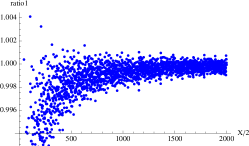
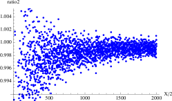
where we have used Eq. (124). Collecting the previous results we get (see Fig. 11-left for a numerical confirmation)

$$\sum_{m=1}^{X}\alpha^{2}(m)\sim\frac{\alpha^{2}}{\alpha_{2}}X-\frac{1}{2}\left(\log X\right)^{2}.$$ (139)

This result is quite different from the one obtained replacing $\alpha^{2}(m)$ by $\langle\alpha(m)\rangle^{2}$ using Eq. (128),

$$\sum_{m=1}^{X}\langle\alpha(m)\rangle^{2}\sim X-\log X+{\rm cte},$$ (140)

which is a consequence of the fluctuations of $\alpha(m)$. In other words, the sum in Eq. (139), provides further information about the distribution of prime numbers.

Let us now consider the second term of Eq. (130), that using Eq. (119) becomes

$$\sum_{m=1}^{X}m\,\alpha^{2}(m) = 2\alpha^{2}\sum_{i=1}^{[X/2]}\sum_{d_{1}|i}\sum_{d_{2}|i}i\,\beta(d_{1})\beta(d_{2}).$$ (141)

Similarly to Eq. (132), one finds

$$\sum_{i=1}^{[X/2]}i|_{{\rm lcm}(d_{1},d_{2})|i} = \frac{\ell_{12}}{2}\left(1+\left[\frac{X}{2\,\ell_{12}}\right]\right)\left[\frac{X}{2\,\ell_{12}}\right],\quad\ell_{12}={\rm lcm}(d_{1},d_{2})$$

$$= \frac{1}{2}\left[\frac{X^{2}}{4\ell_{12}}+X\left(1-2\left\{\frac{X}{2\,\ell_{12}}\right\}\right)+\ell_{12}\left\{\frac{X}{2\,\ell_{12}}\right\}\left(\left\{\frac{X}{2\,\ell_{12}}\right\}-1\right)\right]$$

In this expression we keep the term $O(X^{2})$ and drop the next ones that a numerical calculation show they are $O(X)$. We are led then to the approximation

$$\sum_{m=1}^{X}m\,\alpha^{2}(m) \sim \frac{\alpha^{2}}{4}X^{2}\sum_{d_{1},d_{2}=1}^{\infty}\frac{\beta(d_{1})\beta(d_{2})}{{\rm lcm}(d_{1},d_{2})}+O(X)=\frac{\alpha^{2}}{2\alpha_{2}}X^{2}+O(X)$$ (143)

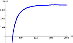
where we used Eq. (134). See Fig. 11 (right) to verify numerically this equation. Finally, Eqs. (139) and (143) implies the asymptotic behavior of Eq. (130)

$$\sum_{i,j=1}^{X/2}\alpha^{2}(2|i-j|)\simeq\frac{\alpha^{2}}{2\alpha_{2}}X^{2}-\frac{X}{2}\left(\log X\right)^{2}+O(X),\quad X\rightarrow\infty.$$ (144)

Fig. 11 (right) shows a numerical check of this relation, that exhibit smaller fluctuations as the previous approximations Eqs. (139) and (143). This is probably due to the fact that they contribute with opposite sign to Eq. (130). For larger values of $X$, not shown in Fig. 11 (right), the result becomes asymptotically exact.

Appendix A4: a toy density matrix

Let us suppose a density matrix of dimension $d$ of the form

$$\rho=\frac{1}{d}({\bf 1}+cP),$$ (145)

where $P$ is the matrix

$$P_{a,a^{\prime}}=\left\{\begin{array}[]{cc}0,&{\rm if}\,a=a^{\prime}\\ 1,&{\rm if}\,a\neq a^{\prime}\\ \end{array}\right..$$ (146)

The eigenvalues of $P$ are

$$p_{1}=d-1,\qquad p_{i}=-1,\;i=2,\dots,d-1.$$ (147)

Hence the eigenvalues of $\rho$ are

$$\lambda_{1}=\frac{1+c(d-1)}{d},\qquad\lambda_{i}=\frac{1-c}{d},\;i=2,\dots,d-1.$$ (148)

The condition $0\leq\lambda_{i}\leq 1$ imposes that $0\leq c\leq 1$. In the limit $d\gg 1$, the purity behaves as

$${\rm Tr}\rho^{2}=\lambda_{1}^{2}+(d-1)\lambda_{2}^{2}=\left(\frac{1+c(d-1)}{d}\right)^{2}+(d-1)\left(\frac{1-c}{d}\right)^{2}\rightarrow c^{2}+\frac{(1-c)^{2}}{d}\simeq c^{2},$$ (149)

where we used that $0<c<1$. Hence the dominant behavior is controlled by the eigenvalue $\lambda_{1}\simeq c$. We can also get this result from the square of $\rho$,

$$\rho^{2}=\frac{1}{d^{2}}({\bf 1}+2cP+c^{2}P^{2})\Rightarrow{\rm Tr}\rho^{2}=\frac{d+c^{2}d(d-1)}{d^{2}}\rightarrow c^{2},$$ (150)

which shows that the purity comes essentially from the square of the off-diagonal matrix $P$. In the same limit the von Neumann entropy behaves as

$$S^{(1)}=-(\lambda_{1}\log\lambda_{1}+(d-1)\lambda_{2}\log\lambda_{2})\rightarrow-c\log c+(1-c)\log\frac{d}{1-c}\sim(1-c)\log d.$$ (151)

Hence satisfies a volume law, with a coefficient that depends on the strength of the off diagonal term $P$.

References

- (1) T. M. Apostol, Introduction to Analytic Number Theory, Springer, 1976.
- (2) H. Davenport, Multiplicative Number Theory, Springer-Verlag, New York (1980).
- (3) C. Vafa, “On the future of mathematics/physics interactions” in Mathematics: Frontiers and Perspectives, Eds. V. Arnold, M. Atiyah, P. Lax and B.Mazur, IMU, AMS (1999).
- (4) D. Schumayer, D. A. W. Hutchinson, “Physics of the Riemann Hypothesis”, Rev. Mod. Phys. 83, 307 (2011);
- (5) M. Watkins, Number Theory and Physics arxiv: http://empslocal.ex.ac.uk/people/staff/mrwatkin//zeta/physics.htm
- (6) B. Julia, “Statistical theory of numbers, in Number Theory and Physics”, eds. J. M. Luck, P. Moussa, and M. Waldschmidt, Springer Proceedings in Physics, Vol. 47, 276, Springer-Verlag, Berlin, 1990
- (7) D. Spector, “Supersymmetry and the Moebius Inversion Function”, Commun. Math. Phys. 127 , 239 (1990).
- (8) I. Bakas and M. J. Bowick, “Curiosities of Arithmetic Gases”, J. Math. Phys. 32, 1881 (1991).
- (9) R. Hagedorn, “Hadronic matter near the boiling point”, Nuovo Cimento 56A, 1027 (1968).
- (10) M. V. Berry, “Riemann’s zeta function: a model for quantum chaos?”, in Quantum Chaos and Statistical Nuclear Physics, edited by T. H. Seligman and H. Nishioka, Springer Lecture Notes in Physics Vol. 263 , p. 1, Springer, New York (1986).
- (11) J. P. Keating, “Periodic orbits, spectral statistics and the Riemann zeros”, in Supersymmetry and Trace Formulae: Chaos and Disorder, eds. I. V. Lerner, J. P. Keating & D. E. Khmelnitskii (Plenum Press), 1-15 (1999).
- (12) E. Bogomolny, “Quantum and Arithmetical Chaos”, in Frontiers in Number Theory, Physics and Geometry, Les Houches, 2003; arXiv:nlin/0312061.
- (13) M. V. Berry, “Hearing the music of the primes: auditory complementarity and the siren song of zeta”, J. Phys. A: Math. Theor. 45 382001 (2012).
- (14) M. du Satoy, The Music of the Primes, NewYork:HarperCollins (2003).
- (15) E. Bombieri, “Prime territory: exploring the infinite landscape at the base of the number system”, The Sciences 32, 30 (1992).
- (16) H. Montgomery “The pair correlation of the zeta function”, in: Proc. Sympos. Pure Math. vol. XXIV, St. Lois. Mo. 1972 . Amer. Math. Soc., Providence, R.I. (1973).
- (17) H. L. Montgomery, “Distribution of the zeros of the Riemann zeta function”, in Proceedings Int. Cong. Math. Vancouver 1974, Vol. I, Canad. Math. Congress, Montreal, 379 (1975).
- (18) A. M. Odlyzko, “Supercomputers and the Riemann zeta function”, in Supercomputing 89: Supercomputing Structures & Computations, Proc. 4-th Intern. Conf. on Supercomputing, International Supercomputing Institute, St. Petersburg, FL, 348 (1989).
- (19) A. Odlyzko, “The zero of the Riemann zeta function and 70 million of its neighbours”, www.dtc.umn.edu/?odlyzko/unpublished. Preprint 1989.
- (20) M. C. Gutzwiller, “Periodic Orbits and Classical Quantization Conditions”, J. Math. Phys. 12, 343 (1971).
- (21) O. Bohigas and M. J. Gianonni, in Mathematical and Computational Methods in Nuclear Physics, edited H. Araki, J. Ehlers, K. Hepp, R. Kippenhahn, H. Weidenmuller and J. Zittart (Springer Verlag, Berlin, 1984).
- (22) J. P. Keating, “Quantum chaology and the Riemann zeta-function”, in Quantum Chaos, eds. G. Casati, I. Guarneri, and U. Smilansky, (North-Holland, Amsterdam), 145, 1993.
- (23) E. B. Bogomolny and J. P. Keating, “Random matrix theory and the Riemann zeros I: three- and four-point correlations”, Nonlinearity 8, 1115, 1995; ibid Random matrix theory and the Riemann zeros II: n-point correlations, Nonlinearity 9, 911, 1996.
- (24) E. B. Bogomolny and J. P. Keating, “Gutzwiller Trace Formula and Spectral Statistics: Beyond the Diagonal Approximation”, Phys. Rev. Lett. 77, 1472, (1996).
- (25) M. V. Berry and J. P. Keating, “The Riemann zeros and eigenvalue asymptotics”, SIAM Review, 41, 236, 1999.
- (26) J.P. Keating and N.C. Snaith, “Random matrices and L-functions”, J. Phys. A: Math. Gen., 36, 2859 (2003).
- (27) J. P. Keating and F. Mezzardi, “Entanglement in quantum spin chains, symmetry classes of random matrices, and conformal field theory”, Phys. Rev. Lett. 94, 050501 (2005).
- (28) E. B. Bogomolny and J. P. Keating, “Two-point correlation function for Dirichlet L-functions”, J. Phys. A: Math. Theor. 46, 095202 (2013);
- (29) M. L. Mehta, Random Matrices, Elsevier Ltd. The Netherlands, 2004.
- (30) M.V. Berry and J.P. Keating, ” and the Riemann zeros”, in Supersymmetry and Trace Formulae: Chaos and Disorder, ed. J.P. Keating, D.E. Khmelnitskii and I. V. Lerner, Kluwer 1999.
- (31) A. Connes, “Trace formula in noncommutative geometry and the zeros of the Riemann zeta function”, Selecta Mathematica New Series 5, 29 (1999). math.NT/9811068.
- (32) B. Aneva, ”Symmetry of the Riemann operator”, Phys. Lett. B 450, 388 (1999).
- (33) G. Sierra, ” with interaction and the Riemann zeros”, Nucl. Phys. B 776, 327 (2007); math-ph/0702034.
- (34) G. Sierra, ”A quantum mechanical model of the Riemann zeros”, New J. Phys. 10, 033016 (2008); arXiv:0712.0705.
- (35) J. C. Lagarias, ”The Schroëdinger operator with Morse potential on the right half line”, Communications in Number Theory and Physics 3 (2009), 323; arXiv:0712.3238.
- (36) J-F. Burnol, ”On some bound and scattering states associated with the cosine kernel”, arXiv:0801.0530.
- (37) G. Sierra and P.K. Townsend, ”The Landau model and the Riemann zeros”, Phys. Rev. Lett. 101, 110201 (2008); arXiv:0805.4079.
- (38) S. Endres and F. Steiner, ”The Berry-Keating operator on and on compact quantum graphs with general self-adjoint realizations”, J. Phys. A: Math. Theor. 43, 095204 (2010); arXiv:0912.3183.
- (39) G. Regniers and J. Van der Jeugt, ”The Hamiltonian and classification of representations”, Workshop Lie Theory and Its Applications in Physics VIII (Varna, 2009); arXiv:1001.1285.
- (40) E. de Rafael, “Large-Nc QCD, Harmonic Sums and the Riemann Zeros”, Nucl. Phys. Proc. Suppl. 207, 290 (2010); arXiv:1010.4657.
- (41) G. Sierra and J. Rodriguez-Laguna, ”The model revisited and the Riemann zeros”. Phys. Rev. Lett. 106, 200201 (2011); arXiv:1102.5356
- (42) M. Srednicki, ”The Berry-Keating Hamiltonian and the Local Riemann Hypothesis”, J. Phys. A: Math. Theor. 44, 305202 (2011); arXiv:1104.1850.
- (43) M. Srednicki, ”Nonclasssical Degrees of Freedom in the Riemann Hamiltonian”, Phys. Rev. Lett. 107, 100201 (2011); arXiv:1105.2342.
- (44) G. Sierra, ”General covariant models and the Riemann zeros”, J. Phys. A: Math. Theor. 45, 055209 (2012); arXiv:1110.3203.
- (45) M. V. Berry and J. P. Keating, ”A compact hamiltonian with the same asymptotic mean spectral density as the Riemann zeros”, J. Phys. A: Math. Theor. 44, 285203 (2011).
- (46) K. S. Gupta, E. Harikumar and A. R. de Queiroz, ”A Dirac type -Model and the Riemann Zeros”, Eur. Phys. Lett. 102, 10006 (2013); arXiv:1205.6755.
- (47) J. C. Andrade, “Hilbert-Polya conjecture, zeta-functions and bosonic quantum field theories”, Int. J. Mod.Phys. A28, 1350072 (2013); arXiv:1305.3342.
- (48) R. V. Ramos and F. V. Mendes, “Riemannian Quantum Circuit”, arXiv:1305.3759.
- (49) M. C. Nucci, ”Spectral realization of the Riemann zeros by quantizing : the Lie-Noether symmetry approach”, J. of Phys: Conf. Series 482, 012032 (2014).
- (50) G. Mussardo, “The quantum mechanical potential for the prime numbers”; cond-mat.9712010.
- (51) H. Wu and D. W. L. Sprung, “Riemann zeros and a fractal potential”, Phys. Rev. E 48, 2595 (1993).
- (52) A. Ramani, B. Grammaticos, and E. Caurier, “Fractal potentials from energy levels”, Phys, Rev. E 51, 6323 (1995).
- (53) B. P. van Zyl and D. A. W. Hutchinson, “Riemann zeros, prime numbers, and fractal potentials”, Physical Review E, 67, 066211 (2003).
- (54) D. Schumayer, B. P. van Zyl, P. Brandon and D. A. W. Hutchinson, “Quantum mechanical potentials related to the prime numbers and Riemann zeros”, Phys. Rev. E 78, 056215 (2008).
- (55) J. I. Latorre and G. Sierra, “Quantum Computation of Prime Number Functions”, Quant. Inf. and Comp., 14, 0577 (2014).
- (56) H. M. Edwards, Riemann’s Zeta Function, Academic Press, New York, 1974.
- (57) P. W. Shor, “Polynomial-Time Algorithms for Prime Factorization and Discrete Logarithms on a Quantum Computer”, SIAM J. Comput. 26, 1484 (1997).
- (58) L. K. Grover, “A fast quantum mechanical algorithm for database search”, Proc. 28th Annual ACM Symposium on Theory of Computing (1996).
- (59) M. A. Nielsen and I. L. Chuang, Quantum Computation and Quantum Information, Cambridge University Press (2000).
- (60) L. Amico, R. Fazio, A. Osterloh, and V. Vedral, “Entanglement in many-body systems”, Rev. Mod. Phys. 80, 517 (2008).
- (61) J. Eisert, M. Cramer, and M. B. Plenio, “Area laws for the entanglement entropy - a review”, Rev. Mod. Phys. 82, 277 (2010).
- (62) L. Masanes, “Area law for the entropy of low-energy states”, Phys. Rev. A, 80, 052104 (2009).
- (63) D. N. Page, “Average entropy of a subsystem”, Phys. Rev. Lett. 71, 1291 (1993); gr-qc/9305007; I. Bengtsson and K. Zyczkowski, Geometry of Quantum States: An Introduction to Quantum Entanglement, Cambridge University Press 2006.
- (64) D. N. Page, “Information in black-hole radiation”, Phys. Rev. Lett. 71, 3743 (1993).
- (65) G. H. Hardy and J. E. Littlewood, “Some Problems of Partition Numerorum. III. On the Expression of a Number as a Sum of Primes”, Acta Math. 44, 1 (1923).
- (66) P. Billingsley, “Prime numbers and Brownian motion”, Amer. Math. Mon. 80, 1099 (1973).
- (67) J. B. Bost and A. Connes, “Hecke Algebras, Type III factors and phase transitions with spontaneous symmetry breaking in number theory”, Selecta Math. (New Series), 1, 411 (1995).
- (68) B. Cipra, “Mathematics - Prime formula weds number theory and quantum physics”, Science, 274, 2014 (1996).
- (69) A. Knauf, “Number theory, dynamical systems and statistical mechanics”, Rev. Mod. Phys. 11, 1027 (1998).
- (70) M. Wolf, “Applications of statistical mechanics in number theory”, Physica A 274, 149 (1999).
- (71) P. Etingof, A. Soloviev and R. Guralnick, “Indecomposable set-theoretical solutions to the quantum Yang-Baxter equation on a set with a prime number of elements”, J. of Algebra, 242, 709 (2001).
- (72) H. C. Rosu, “Quantum Hamiltonians and prime numbers”, Mod. Phys. Lett. A 18, 1205 (2003).
- (73) A. Connes and M. Marcolli, “From Physics to Number Theory via Noncommutative Geometry. Part I: Quantum Statistical Mechanics of Q-lattices”, arXiv:math/0404128.
- (74) A. Sugamoto. “Factorization of number into prime numbers viewed as decay of particle into elementary particles conserving energy”, Prog. of Theo. Phys. , 121, 275 (2009).
- (75) B. Holdom, ”Scale invariant correlations and the distribution of prime numbers” J. Phys. A: Math. Theor. 42, 345102 (2009); arXiv:0903.2592.
- (76) M.V. Suslov, G. B. Lesovik, and G. Blatter, “Quantum Abacus for counting and factorizing numbers”, arXiv:1011.3646.
- (77) M. A. Sanchis-Lozano, J. G. Fernando Barbero and J. Navarro-Salas, “Prime numbers, quantum field theory and the Goldbach conjecture”, Int. Jour. Mod. Phys. A 27, 1250136 (2012); arXiv:1201.6541.
- (78) G. Menezes and N. F. Svaiter, “Quantum Field Theories and Prime Numbers Spectrum”, arXiv:1211.5198.
- (79) K. Chakraborty, A. Chattopadhyay, and P. Poddar, “Primality Testing in Quantum Domain”, preprint 2013.
- (80) M. Wolf, ”Nearest neighbor spacing distribution of prime numbers and quantum chaos”, Phys. Rev. E 89, 022922 (2014); arXiv:1212.3841.
- (81) G. García-Pérez, M. A. Serrano and M. Boguna “The complex architecture of primes and natural numbers”, arXiv:1402.3612.
- (82) J. E. Littlewood, “Sur la distribution des nombres premiers”, Comptes Rendus 158, 1869 (1914).
- (83) H. von Koch, “Sur la distribution des nombres premiers”, Acta Mathematica 24, 159 (1901).
- (84) L. Schoenfeld, “Sharper bounds for the Chebyshev functions and . II”, Mathematics of Computation 30, 337 (1976).
- (85) M. Agrawal, N. Kayal and N. Saxena, ”Primes is in P”, Ann. Math. 160, 781 (2004).
- (86) G. L. Miller, “Riemann’s Hypothesis and Tests for Primality”, J. Comp. and Sys. Sciences. 13, 300 (1976); M. O. Rabin, “Probabilistic algorithm for testing primality”, J. of Number Theory 12, 128 (1980).
- (87) G. Brassard, P. Høyer and A. Tapp, “Quantum Counting”, ICALP’98, Springer-Verlag, LNCS 1443, 820 (1998).
- (88) J. C. Lagarias, V. S. Miller and A. M. Odlyzko, “Computing : The Meissel-Lehmer Method.” Math. Comp. 44, 537 (1985).
- (89) J. C. Lagarias and A. M. Odlyzko, “Computing : An Analytic Method.” J. Algorithms 8, 173 (1987).
- (90) D. J. Platt, “Computing Analytically”, arXiv:1203.5712. To appear in Math. Comp., 2014.
- (91) C. Holzhey, F. Larsen, and F. Wilczek, “Geometric and Renormalized Entropy in Conformal Field Theory”, Nucl. Phys. B 424, 443 (1994).
- (92) G. Vidal, J. I. Latorre, E. Rico and A. Kitaev, “Entanglement in quantum critical phenomena”, Phys. Rev. Lett. 90, 227902 (2003); J. I. Latorre, E. Rico and G. Vidal, “Ground state entanglement in spin chains”, Quantu. Inf. Comp. 4, 48 (2004); J. I. Latorre and A. Riera, J. “A short review on entanglement in quantum spin systems”, Phys. A: Math. Theor. 42, 504002 (2009).
- (93) P. Calabrese and J. Cardy, “Entanglement entropy and quantum field theory”, J. Stat. Mech.: Theory and Experiment, P06002 (2004).
- (94) Hui Li and F. D. M. Haldane, “Entanglement Spectrum as a Generalization of Entanglement Entropy: Identification of Topological Order in Non-Abelian Fractional Quantum Hall Effect States”, Phys. Rev. Lett. 101, 010504 (2008).
- (95) J. I. Cirac and F. Verstraete, “Renormalization and tensor product states in spin chains and lattices”, J. Phys. A: Math. Theor. 42, 504004 (2009); arXiv:0910.1130.
- (96) E. C. Tichmarsh, “The zeros of the Riemann zeta function”, Proc. Royal Soc. London, A- Mathematical and Physical Sciences, vol. 151, 1935.