Temperature Fluctuations as a Source of Brown Dwarf Variability

Abstract

A number of brown dwarfs are now known to be variable with observed amplitudes as large as 10–30% at some wavelengths. While spatial inhomogeneities in cloud coverage and thickness are likely responsible for much of the observed variability, it is possible that some of the variations arise from atmospheric temperature fluctuations instead of, or in addition to, clouds. To better understand the role that thermal variability might play we present a case study of brown dwarf variability using a newly-developed one-dimensional, time-stepping model of atmospheric thermal structure. We focus on the effects of thermal perturbations, intentionally simplifying the problem through omission of clouds and atmospheric circulation. Model results demonstrate that thermal perturbations occurring deep in the atmosphere (at pressures greater than 10 bar) of a model T-dwarf can be communicated to the upper atmosphere through radiative heating via the windows in near-infrared water opacity. The response time depends on where in the atmosphere a thermal perturbation is introduced. We show that, for certain periodic perturbations, the emission spectrum can have complex, time- and wavelength-dependent behaviors, including phase shifts in times of maximum flux observed at different wavelengths. Since different wavelengths probe different levels in the atmosphere, these variations track a wavelength-dependent set of radiative exchanges happening between different atmospheric levels as a perturbation evolves in time. We conclude that thermal—as well as cloud—fluctuations must be considered as possible contributors to the observed brown dwarf variability.

1 Introduction

After more than a decade and a half of surveys for brown dwarf variability we now know that the emergent spectrum of many L- and T- type brown dwarfs indeed varies with time (e.g., Tinney & Tolley, 1999; Bailer-Jones & Mundt, 1999; Artigau et al., 2009; Radigan et al., 2012; Buenzli et al., 2013). Broadband, near-infrared flux variations can be as large as 10–30%, can occur on timescales from 1–100 hours, and can be non-periodic (Bailer-Jones & Mundt, 2001; Gelino et al., 2002; Artigau et al., 2009; Radigan et al., 2012; Gillon et al., 2013). Spectroscopic and multi-band photometric studies have revealed complex, wavelength-dependent lightcurves (Radigan et al., 2012; Buenzli et al., 2013). In some cases, spectra show periodic brightness fluctuations with wavelength-dependent phase lags, which can be as large as 180^∘ (i.e., shifted by half of a cycle) (Buenzli et al., 2012).

Clouds sculpt the emergent spectra of essentially all spectral classes of brown dwarfs, although their impact is most notable in the L-dwarfs (Leggett et al., 1998; Chabrier et al., 2000; Allard et al., 2001; Ackerman & Marley, 2001; Tsuji, 2002; Golimowski et al., 2004; Knapp et al., 2004; Burrows et al., 2006; Stephens et al., 2009; Morley et al., 2012). Given the strong evidence for the presence of clouds in brown dwarf atmospheres, and the ability of a continuum opacity source to limit the depth of the wavelength-dependent photosphere (Ackerman & Marley, 2001), it is expected that these structures play some role in brightness variability (Radigan et al., 2012; Apai et al., 2013). Indeed thermal emission from the deep atmospheres of both Jupiter and Saturn is strongly modulated by cloud structures and Jupiter itself would show substantial variability if the disk were observed at 5 $\mu$m in integrated light (Gelino & Marley, 2000). However the intensity of radiation emitted by a planetary or brown dwarf atmosphere depends on many factors in addition to cloud structure. Atmospheric temperature and composition also control the thermal emission and it seems prudent to also consider the role such factors might contribute to variability.

Freytag et al. (2010) used a 2-D radiation hydrodynamics model to study atmospheric circulation and dust transport in M-dwarf and brown dwarf atmospheres. This work highlighted the importance of gravity waves and dust convection to maintaining clouds in brown dwarf atmospheres. They found that gravity waves are expected to be ubiquitous above the radiative-convective boundary and likely play an important role in cloud development and evolution. More recently, global 3-D, cloud-free models were used by Showman & Kaspi (2013) to study large-scale flows and convection in the interiors and deep atmospheres of brown dwarfs. These models revealed that convection is strongly influenced by the relatively fast rotation rates of brown dwarfs and that thermal variations of order several Kelvin may be expected at the top of the model convective zone. This work also discussed a stratospheric circulation, driven by the interaction between atmospheric waves generated at the top of the convective zone and the mean stratospheric flow, that could lead to large ($\sim$50 K) temperature variations in the upper atmospheres of brown dwarfs. However, emission spectra were not computed, and so the influence of these variations on the brown dwarfs’ spectra remain unclear.

Here we provide a case study of the impact of atmospheric temperature fluctuations on the emission spectrum of a brown dwarf. We intentionally simplify the problem by neglecting clouds as well as chemical evolution, thus allowing us to explore the behaviors, timescales, and related spectral variability due to temperature fluctuations alone. Using a new 1-D, time-stepping radiative convective model for brown dwarfs, we first investigate the heating of an atmosphere due to an extended thermal pulse from deep within the convective zone. We then explore variability in the emission spectrum due to time-varying thermal fluctuations, introducing these perturbations at different atmospheric levels, and highlighting circumstances where the model can reproduce wavelength-dependent phase lags.

2 Model Description

We adapt a well-validated thermal structure model of brown dwarfs (Marley et al., 1996, 2002) to permit realistic time-stepping, thus permitting studies of the time-dependent evolution of atmospheric thermal pulses. We take the atmosphere to be in hydrostatic equilibrium. The heating rate, $Q$, throughout the atmospheric profile is given by

$$Q=\frac{dT}{dt}=\frac{g}{c_{p}}\frac{dF_{\text{net}}}{dp}\ ,$$ (1)

where $T$ is temperature, $t$ is time, $g$ is the acceleration due to gravity, which we take to be constant over the small range of altitudes encompassed by the atmosphere, $c_{p}$ is the temperature- and pressure-dependent specific heat capacity, $F_{\text{net}}$ is the net energy flux, carried by both radiation and convection, and $p$ is pressure. Values for the specific heat are taken from the equation of state models of Saumon et al. (1995).

Gas opacities in our model are computed according to Freedman et al. (2008), and chemical abundances of all radiatively active species are provided by the equilibrium models of Lodders (2004) and Lodders & Fegley (2006). For a given pressure-temperature ($p$-$T$) profile and set of gas composition profiles, the upwelling and downwelling thermal fluxes are computed for 180 wavelength bins, spanning 0.4–325 $\mu$m. Within each spectral interval, the two-stream source function technique (Toon et al., 1989) is used to solve the equation of radiative transfer within discrete spectral bins using eight-term, correlated-$k$ coefficients.

The convective heat flux, $F_{c}$, is computed according to mixing length theory (Vitense, 1953; Gierasch & Goody, 1968), and is given as

$$F_{c}=-\rho c_{p}K_{H}\left(\frac{dT}{dz}+\Gamma_{\text{ad}}\right)\ ,$$ (2)

where $\rho$ is the mass density, $K_{H}$ is the eddy diffusivity for heat, $z$ is altitude, and $\Gamma_{\text{ad}}=g/c_{p}$ is the adiabatic lapse rate. The eddy diffusivity vanishes when the temperature profile is stable against convection, and is given by

$$K_{H}=\begin{cases}l^{2}\left[\frac{g}{T}\left(\frac{dT}{dz}+\Gamma_{\text{ad}}\right)\right]^{1/2},&\frac{dT}{dz}>-\Gamma_{\text{ad}}\\ 0,&\frac{dT}{dz}\leq-\Gamma_{\text{ad}}\end{cases}$$ (3)

where $l$ is the mixing length, which we set equal to the pressure scale height, $H$, with

$$l=H=\frac{k_{B}T}{\mu g}\ ,$$ (4)

where $k_{B}$ is the Boltzmann constant, and $\mu$ is the atmospheric mean molecular mass. We tested sensitivity to our mixing length parameterization by running simulations with $l=2H$ and $l=\frac{1}{2}H$, and found negligible differences in model outputs.

Time-stepping in our model proceeds in a straightforward, linear fashion. A time increment, $\Delta t$, is selected that is short enough to maintain stability in the convective region of the atmosphere. Typically, $\Delta t$ of order 0.1–1 s suffices, which is about 1/10 of the convective timescale for a single model layer. Given a $p$-$T$ profile at time $t$, the temperature at level $i$ is updated according to

$$T_{i}\left(t+\Delta t\right)=T_{i}\left(t\right)+Q_{i}\Delta t\ ,$$ (5)

where $Q_{i}$ is the heating rate at model pressure level $i$. Our pressure grid contains 68 levels between 90 bar and $3\times 10^{-4}$ bar which are, roughly, equally spaced in log-pressure. The wall-clock time of each model time-step is much less than one second, due to the computational efficiency of our radiation and convection schemes. We verified that the time-stepping model’s equilibrium $p$-$T$ curve and depth of the convective zone agreed with previous versions of our model, which found equilibrium solutions using a Newton-Raphson technique.

In this case study, we use a model T dwarf with an effective temperature of 900 K and a surface gravity of $10^{5}$ cm s^-2. This set of parameters was previously found to produce steady-state models that reproduce observations of a variable T6.5 brown dwarf, 2MASS J22282889–431026 (Buenzli et al., 2012). Note that the best-fit models for this case included thin clouds of Na₂S, MnS, and Cr, which, as mentioned earlier, we intentionally omit.

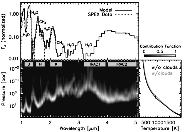
Figure 1 shows the modeled emission spectrum, wavelength- and pressure-dependent normalized contribution functions (Hanel et al., 1992, p. 131), and equilibrium $p$-$T$ profile for this object, and also shows the observed SPEX spectrum (Burgasser et al., 2004). The contribution functions show the range of pressures that contribute information to the top-of-atmosphere spectrum (i.e., the wavelength-dependent specific flux exiting the atmosphere to space), and the pressure at the base of the atmospheric simulations was chosen to extend below the deepest pressures probed by the spectra (which occurs primarily at visible wavelengths). Relevant near-infrared bandpasses are also shown, which, for example, demonstrate that the IRAC1 filter is sensitive to lower pressures (higher altitudes) than is J-band. Small discrepancies at continuum wavelengths between the modeled and observed spectra are due to our omission of clouds. For comparison, Figure 1 also shows a $p$-$T$ profile from a cloudy model (Morley et al., 2012) that was shown to reproduce a time-averaged spectrum of the aforementioned 2MASS object in Buenzli et al. (2012). As was shown in Buenzli et al. (2012), models of this object that include clouds place these relatively deep in the atmosphere, with several different cloud decks forming below 2 bar. Our contribution functions demonstrate that there are wavelength regions below 1.7 $\mu$m (between the strong water bands) which are sensitive to these pressures. As a result, a model spectrum that includes clouds has less flux at these continuum wavelengths.

3 Results

We proceed with two key investigations in our case study. First, we use our time-stepping model to study the monotonic heating of a brown dwarf atmosphere due to an energy source at depth. The focus of this investigation is to understand how the deep atmosphere communicates energy to the upper, radiatively-dominated levels of the atmosphere. Second, we introduce periodic perturbations at different levels of the atmosphere. We do not specify the mechanism driving these fluctuations, but energy sources could include dynamics, atmospheric wave breaking (e.g., Young et al., 1997), cloud radiative and latent heating affects, and/or other processes. As different wavelengths in the top-of-atmosphere spectrum probe different pressures, we show how the time-dependent perturbations lead to complex behavior in the emergent spectrum.

3.1 Time-Dependent Response to Heating at Depth

We can gain insight into the time-dependent response of a brown dwarf atmosphere to a perturbation by varying the bottom boundary condition, which is the internal heat flux. This flux is equal to $\sigma T_{\text{eff}}^{4}$, where sigma is the Stefan-Boltzmann constant, and $T_{\text{eff}}$ is the dwarf’s effective temperature. For our $T_{\text{eff}}=900$ K body, this flux is nominally $3.72\times 10^{4}$ W m^-2. We study the response of the atmosphere, initially in equilibrium, to a 10% increase in this flux, to $4.09\times 10^{4}$ W m^-2 (or $T_{\text{eff}}=922$ K).

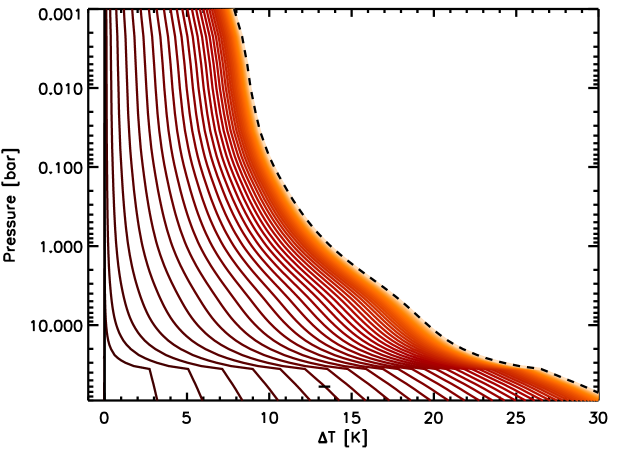
Figure 2 shows the time-dependent evolution of atmospheric temperatures, relative to the equilibrium profile shown in Figure 1. A curve is shown for every 20 hours of evolution, and brighter hues show later times. The convective portion of the atmosphere, which is below 40 bar, heats nearly uniformly, while the upper portions of the atmosphere lag behind, which is because the convective timescale ($\sim$0.1–1 hours) is short compared to the radiative timescale ($\sim$10–100 hours). Note that the new equilibrium temperatures, shown by the dashed curve, are about 1–2% larger than the initial equilibrium state. Also, this figure demonstrates that the characteristic timescale at which the atmosphere responds to the perturbation at depth is $\sim 100$ hours.

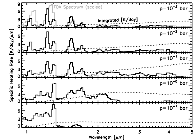
Despite the perturbation being introduced at the base of the atmosphere, at 90 bar, we see that the upper atmosphere is already beginning to heat by several tens of hours into the simulation, and achieves its maximum heating rate at about 120 hours into the simulation. To understand this behavior, we investigated the wavelength- and pressure-dependent radiative heating rates at 120 hours into the run. These are shown in Figure 3. Here, different vertical sub-figures are for different pressures in the atmosphere, at $10^{-3}$, $10^{-2}$, $10^{-1}$, $1$, and $10$ bar. The horizontal axis is wavelength, and the vertical axis is the specific heating rate (in K day^-1 $\mu$m^-1). The dotted curve is the integrated heating rate, (in K day^-1). For convenience, a scaled version of the top-of-atmosphere spectrum is shown in light grey in the top sub-figure.

Investigation of the radiative heating rates in Figure 3 shows that the upper-most portions of the atmosphere are responding to increases in radiative fluxes at short wavelengths (below about 2 $\mu$m). Heating at these levels occurs primarily in the wings of water vapor absorption bands. The opacity at band centers is too large for the upper atmosphere to “see” flux from the deep atmosphere, and there is not enough opacity in window regions at low pressures for significant flux to be absorbed, which would drive heating at these levels.

3.2 Periodic Perturbations at Different Atmospheric Pressures

To investigate periodic variability, we artificially introduce a sinusoidally-varying heating rate to our model atmosphere at different pressures. This perturbation is in addition to the heating/cooling due to gradients in the net radiative and convective fluxes that occur as the atmosphere evolves through time. Thus, Equation 1 is now

$$\frac{dT}{dt}=\frac{g}{c_{p}}\frac{dF_{\text{net}}}{dp}+Q_{f}\sin\left(\frac{2\pi t}{P}\right)\delta\left(p-p_{f}\right)\ ,$$ (6)

where $Q_{f}$ is the amplitude of the fluctuation (in degrees Kelvin per unit time), $P$ is the fluctuation period, $\delta$ is the Dirac delta function, and $p_{f}$ is the pressure where the fluctuation is introduced. In practice, since model levels are discretized, the heating perturbation is introduced over a small range of model pressures. We choose $p_{f}$ as either the base of the atmosphere (near 100 bar), at 10 bar, or at 1 bar, and study the quasi-steady-state behavior over the course of entire fluctuation cycle. The timescales we investigate are 10, 50, 100, and 500 hours, and $Q_{f}$ is selected for each run so that the temperature at the perturbed level varies by 1% over a cycle (i.e., 20 K variation at the base, 13 K at 10 bar, and 8 K at 1 bar). As mentioned earlier, we do not specify the mechanism that drives these fluctuations, but possible sources include dynamics, wave breaking, cloud effects, and/or other processes.

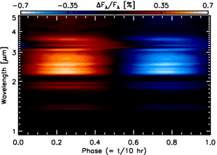
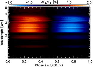
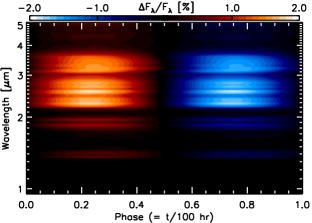
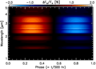
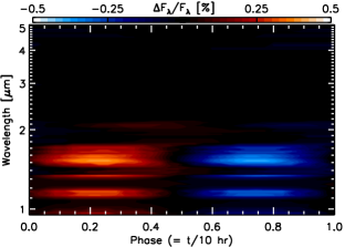
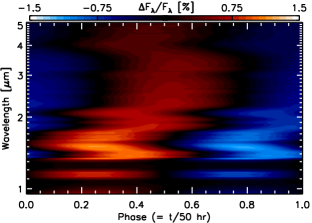
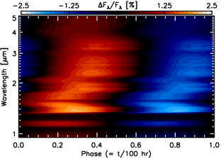
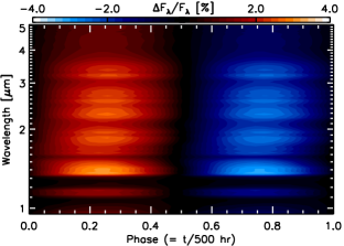
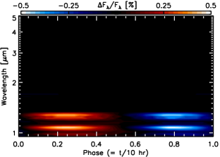
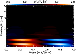
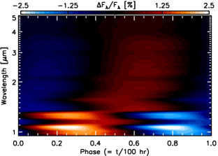
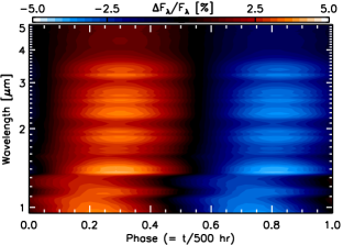
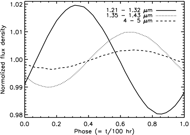
Figure 4 shows a grid of model results for the different perturbation pressures and timescales. The horizontal axis is time, which spans one full perturbation cycle, and the vertical axis is wavelength through the near-infrared. Contours show the relative changes in the brightness of the top-of-atmosphere spectrum ($\Delta F_{\lambda}/F_{\lambda}$, where $F_{\lambda}$ is the brightness averaged over a full cycle). Recall that the contribution functions in Figure 1 allow us to map between wavelength and the pressure levels that contribute flux at that wavelength. A set of lightcurves, from the case with a perturbation introduced at the base of the atmosphere with a period of 100 hours in Figure 4, are shown for several different bandpasses in Figure 5. These bandpasses were chosen as a subset of those used in Buenzli et al. (2012), and highlight the wavelength-dependent phase lag produced by our model.

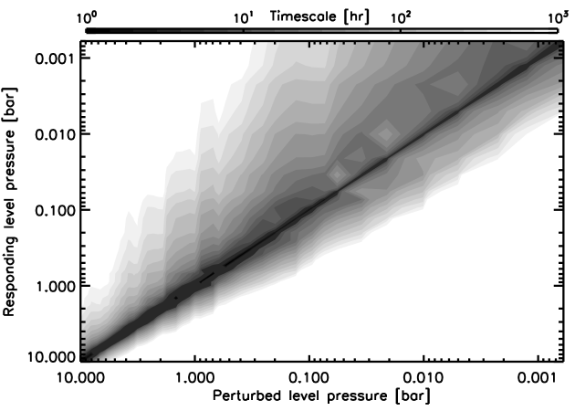
The models with time-varying perturbations demonstrate a number of complex behaviors, including wavelength-dependent phase lags. Of note are the cases where the perturbations are introduced high in the atmosphere (1 bar). Here, regardless of the timescale of the perturbation, the deeper atmospheric levels, which are probed by the shorter wavelengths, do not experience substantial temperature fluctuations, and so we see little or no variability at shorter wavelengths. To understand this behavior, we explore the radiative response timescales in the atmosphere, which are shown in Figure 6. We estimate the timescale at which atmospheric level $i$ responds to a small (1%) temperature increase, $\Delta T$, in level $j$ by computing the profile of net radiative heating in response to this perturbation. This timescale is then

$$\tau_{\text{rad},i}=\frac{\Delta T_{j}}{Q_{\text{rad},i}}\ ,$$ (7)

where $Q_{rad,i}$ is the radiative heating rate at level $i$ after the perturbation is applied. As Figure 6 shows, these timescales are from $\sim$1 hr for levels near the perturbation, to $\sim$$10^{3}$ hr for levels far from the perturbation, with timescales tending to be longer for deep levels responding to perturbations at low pressures.

4 Discussion

Brown dwarf variability is influenced by a number of physical processes, each operating at its own timescale and spatial scale. Commensurate with these variations will be thermal fluctuations, possibly due to convective motions (Showman & Kaspi, 2013), atmospheric wave breaking, or perhaps latent and/or cloud heating effects. The model investigations presented here explore the evolution of such thermal fluctuations.

Our simplest case is an atmosphere heated from below, where the internal heat flux is increased, and the thermal structure is allowed to adjust. Temperatures throughout the column increase by 1–2% on timescales of order 100 hours. As Figure 2 demonstrates, there is clear communication between the deep atmosphere (at pressures larger than $\sim$10 bar) and the upper atmosphere (at pressures smaller than $\sim$0.1 bar). The radiative heating rates (Figure 3) show that a substantial amount of heating in the upper atmosphere is due to radiation absorbed below about 2 $\mu$m. The deep atmosphere, which is at temperatures of 1500-2000 K, contributes substantial thermal emission at these wavelengths (about 40% of the flux from a 1750 K blackbody is emitted shortward of 2 $\mu$m), and the atmosphere is relatively transparent here, too (Figure 1).

Our investigation of heating from below shows that the timescale at which the atmosphere responds is distinct from the level radiative response timescales presented in Figure 6. The latter simply relates a perturbation at a single level to a response timescale at all other atmospheric levels, whereas the former is a phenomenological timescale associated with the communication and passage of a heating (or cooling) pulse through the atmospheric column. When we let a perturbation evolve in time, as when we increase the internal heat flux into the model atmosphere, we see that levels near the perturbed level respond rapidly (at the level radiative response timescale), and this communication is efficiently passed upward through the atmospheric column. Thus, the level radiative response timescales tend to over-estimate the timescales for communicating thermal pulses over large pressure ranges.

A key feature of the radiative response times shown in Figure 6 is their asymmetry in communicating a perturbation upward versus downward through the atmosphere. The deep atmosphere responds more slowly to perturbations above than vice versa. This is, in part, a column mass effect—an equal mass of material (per unit area) is located in a column extending from the top of the atmosphere to 1 bar as is located between 1 bar and 2 bar. Additionally, as was mentioned above, while the deep atmosphere is at high enough temperatures to emit a substantial amount of flux at the short wavelengths where the atmosphere is relatively transparent, the upper atmosphere is too cool to contribute much thermal flux at these wavelengths (less than 1% of the flux from a 500 K blackbody is emitted shortward of 2 $\mu$m).

The role of radiative response timescales, and their asymmetry between the deep atmosphere and the upper atmosphere, is apparent in fluctuations in the top-of-atmosphere spectrum when periodic heating perturbations are imposed at different pressures in our model atmosphere (Figure 4). When the perturbation is introduced at the base of the atmosphere (90 bar), and the perturbation timescale is short ($\lesssim 100$ hr), the upper atmosphere does not respond, and we see no variability in the spectrum between 2–5 $\mu$m (which probe lower pressures in the atmosphere). As the timescale of the perturbation increases, the fluctuations become apparent at lower pressures. For the longest timescale fluctuations investigated here (500 hr), the entire atmosphere column responds nearly in unison to the perturbation at depth.

When the perturbation is introduced at 10 bar, we see that the fluctuations at lower pressures (longer wavelengths) becomes apparent at shorter timescales. We do not see fluctuations near 1.1 and 1.3 $\mu$m, which probe deeper pressures, since the perturbation cannot be communicated as efficiently into the deep atmosphere. Similar behaviors are seen when the perturbation is introduced at 1 bar, except that communication to pressures smaller than this occurs at shorter timescales, and so the fluctuations in the top-of-atmosphere spectrum look similar across a wide range of perturbation timescales.

The asymmetry in radiative response timescales then indicates an important potential observable, since spectral fluctuations due to thermal perturbations at lower pressures will be distinct from those occurring at depth. Specifically, variability at wavelengths that probe the upper atmosphere, and a lack of variability at wavelengths that probe the deep atmosphere, indicates a perturbation occurring higher in the atmosphere. Perturbations occurring at depth will be apparent at the wavelengths that probe higher pressures, and can generate spectral variability at other wavelengths, depending on the timescale of the perturbation.

While the extremes of the response of an atmosphere to a perturbation is uniform heating/cooling (at long timescales) and strictly local heating/cooling (at short timescales), complex behavior arises in between these extremes, and is rooted in the different timescales at which an atmospheric level is responding to perturbations in all other levels. Wavelength-dependent phase lagging is apparent in some cases in Figure 4, primarily at wavelengths below 2 $\mu$m, where the top-of-atmosphere spectrum probes a wide range of pressures over a relatively small range of wavelengths, although phase lags at longer wavelengths are also apparent.

We note that our case with a perturbation introduced at the base of the atmosphere on a timescale of 100 hours produces brightness fluctuations whose wavelength dependence bear a similarity to those observed in Buenzli et al. (2012) (see Figure 5). Like the observations reported by Buenzli et al., the amplitude of the model fluctuations is typically of order 1–3%, and the flux measured in a 1.35–1.43 $\mu$m bandpass lags the flux measured in a 1.21–1.32 $\mu$m bandpass (by 140^∘ in our model, as compared to $\sim$180^∘ in the observations). However, our model cannot explain all of the details of the observations. Most importantly, the brown dwarf varies on roughly hour-long timescales, which is comparable to the rotation period and probably reflects the complex, three-dimensional nature of the atmosphere. In contrast, our model perturbation timescales are closer to 100 hours. This is likely a shortcoming of using a one-dimensional model, although we note that the observations reported by Buenzli et al. (2012) do show brightness trends on timescales longer than 10 hours. Thus, in summary, our results show that thermal fluctuations can be an important aspect of spectral variability, while also pointing to the necessary role of dynamics and clouds in fully explaining observations.

Future studies should examine the interconnected role of thermal perturbations and cloud and chemical evolution on thermal variability. Clouds typically act as a continuum opacity source. Thus, clouds will limit sensitivity to thermal fluctuations occurring in atmospheric layers beneath the cloud base (i.e., those layers probed at window/continuum wavelengths in the cloud-free case), and this effect will be stronger for more optically thick clouds. Alternatively, clouds will shield deeper atmospheric layers from thermal perturbations that are propagating downwards, preventing those layers from heating/cooling as they would in a cloud-free scenario. Of course, clouds are not a steady-state process, and so will respond with their own characteristic timescales when other atmospheric layers are perturbed from their equilibrium state. For example, if an amount of flux, $\Delta F$, across a cloud with column mass $M_{c}$ (analogous to liquid water path for Earth clouds) goes into vaporizing the cloud particles, then a characteristic timescale would be $\tau_{\text{cld}}\sim M_{c}L/\Delta F$, where $L$ is the latent heat of vaporization. Thus, there is the potential for interesting feedbacks to occur, where the atmosphere is attempting to respond at one timescale (like those discussed in this work), while the clouds are evolving at another timescale.

Finally, as the ability of different layers in the atmosphere to influence one another via radiation hinges on the relatively clear opacity spectral windows found in T-dwarf atmospheres. L-dwarfs, with stronger cloud and molecular continuum opacity which partially fill in the spectral windows, may accordingly exhibit less radiative coupling between layers, longer response timescales, and perhaps smaller phase shifts between different spectral bandpasses. Larger systematic surveys into brown dwarf variability should investigate such possibilities, not to mention the three-dimensional roles of atmospheric dynamics as coupled to rotation.

5 Conclusions

Using a one-dimensional model of brown dwarf atmospheric structure, we have studied the time-dependent evolution of the atmosphere in response to a variety of thermal perturbations. We omitted cloud and dynamical effects, choosing to concentrate on behaviors that arise strictly due to atmospheric thermal variations. Thermal perturbations of the deep atmosphere can be communicated to the upper atmosphere at shorter near-infrared wavelengths, although communication in the opposite direction is impeded by the lack of flux generated at these wavelengths by the relatively cool upper atmosphere. The response timescale of the atmosphere to thermal perturbations is typically 10–100 hours. Deep thermal perturbations can lead to brightness fluctuations at nearly all near-infrared wavelengths, and our model predicts that these could be observed on timescales of hundreds of hours. While it is not our goal to solve the entire problem of brown dwarf variability, our model can produce a number of the observed features, depending on the nature of the thermal perturbation. In the future, a full explanation of variability in brown dwarf thermal emission spectra must incorporate three-dimensional atmospheric and cloud dynamics, as well as the time-dependent evolution of thermal perturbations throughout the radiative portion of the atmosphere.

Figure 1: Top-of-atmosphere spectrum, contribution functions, and thermal structure for the equilibrium state of the brown dwarf used in this case study ($T_{\text{eff}}=900$ K, $g=10^{5}$ cm s^-2). Key absorption features and relevant near-infrared bandpasses are indicated. Also shown are SPEX observations of 2MASS J22282889–431026 (Burgasser et al., 2004), which has been shown to be variable (Buenzli et al., 2012). The model is brighter than the SPEX data at continuum wavelengths due to our omission of clouds. The contribution functions indicate the range of pressures that contribute flux to the top-of-atmosphere spectrum at a given wavelength (model levels are apparent in the shading). The black $p$-$T$ profile is for the standard, cloud-free case used in this study. The convective portion of the atmosphere is shown by a thickened line, and the vertical mark indicates where the atmosphere temperature equals the effective temperature. Also shown is a $p$-$T$ profile (in grey) from a cloudy model(Morley et al., 2012) which was found to reproduce, on average, a spectrum of the aforementioned 2MASS object in Buenzli et al. (2012).

Figure 2: Time-dependent heating of model atmosphere in response to an increase in the internal heat flux, which was increased by 10% from $3.72\times 10^{4}$ W m^-2 to $4.09\times 10^{4}$ W m^-2. Temperatures are relative to the equilibrium state shown in Figure 1. Curves are separated by 20 hours, brighter hues are for later times, and a total elapsed time of 1000 hours is shown. Note the different behaviors in the convective region and the radiative region, where the radiative-convective boundary is at 40 bar. The dashed line shows the new equilibrium state, where temperatures are 1–2% greater than their initial values. The horizontal tick mark indicates the curve for which radiative heating rates are shown in Figure 3.

Figure 3: Wavelength dependent specific heating rates at 120 hours into the simulation shown in Figure 2 (see marked curve in this figure), which is when the radiative heating rates in the upper atmosphere are at their largest. The rates shown here have the initial equilibrium rates subtracted off, and, thus, represent a net heating above the initial state. Different sub-figures are for different pressure levels in the atmosphere, which are indicated in the upper-right. The dotted curve is the running total of the integrated heating rate, which uses the same vertical axis scale. A scaled version of the top-of-atmosphere spectrum is shown in the top sub-panel (in light grey).

(a)

(b)

(c)

(d)

(e)

(f)

(g)

(h)

(i)

(j)

(k)

(l)

Figure 4: Flux variations from time-dependent models where periodic heating perturbations have been introduced at different atmosphere pressures and at different timescales. Rows are for different pressure locations of the perturbation (top - 1 bar, middle - 10 bar, bottom - base of atmosphere), and columns are for different timescales (left - 10 hr, mid-left - 50 hr, mid-right - 100 hr, right - 500 hr). Horizontal axis is time, which covers an entire perturbation cycle, and vertical axis is wavelength. Shading indicates top-of-atmosphere brightness variations relative to their mean state (i.e., averaged over an entire cycle), where red hues are brighter than average, and blue hues are dimmer than average. Note the different relative flux scales indicated at the top of each sub-figure.

Figure 5: Example lightcurves, taken from Figure 4, for the case where a perturbation is introduced at the base of the atmosphere with a period of 100 hours. Three different bandpasses are shown (including IRAC2) that correspond to a subset of those used in (Buenzli et al., 2012), and which highlight the wavelength-dependent phase lag produced by our model.

Figure 6: Atmospheric radiative response timescales. A 1% temperature perturbation is artificially introduced at a model level (the “perturbed level”, horizontal axis), and we estimate a timescale for responding to this perturbation at all other levels (the “responding level”, vertical axis). As the color bar at the top of the plot indicates, timescales range from $\sim$1 hr, for levels near the perturbed level, to $\sim$$10^{3}$ hr for levels that are far from the perturbation.

References

- Ackerman & Marley (2001) Ackerman, A. S., & Marley, M. S. 2001, ApJ, 556, 872
- Allard et al. (2001) Allard, F., Hauschildt, P. H., Alexander, D. R., Tamanai, A., & Schweitzer, A. 2001, ApJ, 556, 357
- Apai et al. (2013) Apai, D., Radigan, J., Buenzli, E., et al. 2013, ApJ, 768, 121
- Artigau et al. (2009) Artigau, É., Bouchard, S., Doyon, R., & Lafrenière, D. 2009, ApJ, 701, 1534
- Bailer-Jones & Mundt (1999) Bailer-Jones, C. A. L., & Mundt, R. 1999, A&A, 348, 800
- Bailer-Jones & Mundt (2001) —. 2001, A&A, 367, 218
- Buenzli et al. (2013) Buenzli, E., Apai, D., Radigan, J., Reid, I. N., & Flateau, D. 2013, ArXiv e-prints, arXiv:1312.5294
- Buenzli et al. (2012) Buenzli, E., Apai, D., Morley, C. V., et al. 2012, ApJ, 760, L31
- Burgasser et al. (2004) Burgasser, A. J., McElwain, M. W., Kirkpatrick, J. D., et al. 2004, AJ, 127, 2856
- Burrows et al. (2006) Burrows, A., Sudarsky, D., & Hubeny, I. 2006, ApJ, 640, 1063
- Chabrier et al. (2000) Chabrier, G., Baraffe, I., Allard, F., & Hauschildt, P. 2000, ApJ, 542, 464
- Freedman et al. (2008) Freedman, R. S., Marley, M. S., & Lodders, K. 2008, ApJS, 174, 504
- Freytag et al. (2010) Freytag, B., Allard, F., Ludwig, H.-G., Homeier, D., & Steffen, M. 2010, A&A, 513, A19
- Gelino & Marley (2000) Gelino, C., & Marley, M. 2000, in Astronomical Society of the Pacific Conference Series, Vol. 212, From Giant Planets to Cool Stars, ed. C. A. Griffith & M. S. Marley, 322
- Gelino et al. (2002) Gelino, C. R., Marley, M. S., Holtzman, J. A., Ackerman, A. S., & Lodders, K. 2002, ApJ, 577, 433
- Gierasch & Goody (1968) Gierasch, P., & Goody, R. 1968, Planet. Space Sci., 16, 615
- Gillon et al. (2013) Gillon, M., Triaud, A. H. M. J., Jehin, E., et al. 2013, A&A, 555, L5
- Golimowski et al. (2004) Golimowski, D. A., Leggett, S. K., Marley, M. S., et al. 2004, AJ, 127, 3516
- Hanel et al. (1992) Hanel, R. A., Conrath, B. J., Jennings, D. E., & Samuelson, R. E. 1992, Exploration of the solar system by infrared remote sensing (Cambridge University Press)
- Knapp et al. (2004) Knapp, G. R., Leggett, S. K., Fan, X., et al. 2004, AJ, 127, 3553
- Leggett et al. (1998) Leggett, S. K., Allard, F., & Hauschildt, P. H. 1998, ApJ, 509, 836
- Lodders (2004) Lodders, K. 2004, Science, 303, 323
- Lodders & Fegley (2006) Lodders, K., & Fegley, Jr., B. 2006, in Astrophysics Update 2, ed. J. W. Mason (Springer-Praxis Books), 1–28
- Marley et al. (1996) Marley, M. S., Saumon, D., Guillot, T., et al. 1996, Science, 272, 1919
- Marley et al. (2002) Marley, M. S., Seager, S., Saumon, D., et al. 2002, ApJ, 568, 335
- Morley et al. (2012) Morley, C. V., Fortney, J. J., Marley, M. S., et al. 2012, The Astrophysical Journal, 756, 172
- Radigan et al. (2012) Radigan, J., Jayawardhana, R., Lafrenière, D., et al. 2012, ApJ, 750, 105
- Saumon et al. (1995) Saumon, D., Chabrier, G., & van Horn, H. M. 1995, ApJS, 99, 713
- Showman & Kaspi (2013) Showman, A. P., & Kaspi, Y. 2013, ApJ, 776, 85
- Stephens et al. (2009) Stephens, D. C., Leggett, S. K., Cushing, M. C., et al. 2009, ApJ, 702, 154
- Tinney & Tolley (1999) Tinney, C. G., & Tolley, A. J. 1999, MNRAS, 304, 119
- Toon et al. (1989) Toon, O. B., McKay, C., Ackerman, T., & Santhanam, K. 1989, Journal of Geophysical Research: Atmospheres (1984–2012), 94, 16287
- Tsuji (2002) Tsuji, T. 2002, ApJ, 575, 264
- Vitense (1953) Vitense, E. 1953, ZAp, 32, 135
- Young et al. (1997) Young, L. A., Yelle, R. V., Young, R., Seiff, A., & Kirk, D. B. 1997, Science, 276, 108