Improved valence PDFs at leading order via connection formulas between the different QCD orders

Abstract

The formulas directly connecting parton distribution functions (PDFs) at the leading (LO) and the next to leading (NLO) QCD orders are applied to both unpolarized and polarized valence PDFs and produce improved LO results on these quantities without exclusion from the analysis the data coming from the small and moderate $Q^{2}$ region. It is shown that derived in this way and presented in the paper improved LO parametrizations of the valence PDFs could be obtained within the standard LO analysis by using only the data produced at very high $Q^{2}$ values (that is hardly possible in reality) and they strongly differ from the original LO parametrizations of these quantities, obtained by using the most of data produced at small and moderate $Q^{2}$ values. It is argued that LO results on PDFs can be significantly improved even if the respective NLO results are still unavailable.

PACS: 13.85.Ni, 13.60.Hb, 13.88.+e

QCD analysis of the experimental data at LO is a very useful tool for the understanding of hadronic high energy reactions. This is due to its simplicity and comprehensiveness as well as to its universality, i.e. applicability to any hadronic process. Of importance is also (and it seems to be the main advantage of LO) that in contrast to PDFs and fragmentation functions (FFs) at higher QCD orders these quantities at LO not only can be used as an input for calculation (in the chosen factorization scheme) of asymmetries and cross sections of different processes, but being scheme independent have the physical meaning themselves, allowing the probabilistic interpretation and, thereby, the possibility of qualitative physical predictions.

All these reasons make LO analysis very needed even today and many modern collaborations produce namely LO results on PDFs/FFs (see, for instance, [1, 2]). Besides, it is of importance also, that until now only LO analysis is still possible (see [3, 4] and references therein) for asymmetries giving access to such intensely studied nowadays PDFs as transverse momentum distributions (TMDs). At the same time, as we will see below, the inclusion of the data produced at small and moderate $Q^{2}$ in the standard LO analysis is really dangerous for the LO results: as we will see below, the difference between the LO results on PDFs with and without inclusion of the small and moderate $Q^{2}$ data into analysis is significant and is not covered by the error band. However, now did appear a good possibility to produce the correct LO results on PDFs/FFs without lost of events collected in experiment at small and moderate $Q^{2}$, which make up the overwhelming majority of events available to any experiment.

Recently [5] the formulas directly connecting parton distribution functions and fragmentation functions at the next to leading order of QCD with the same quantities at the leading order were derived (see Eqs. (15), (16) in Ref. [5]). To obtain these formulas only the DGLAP evolution equations and the asymptotic condition that PDFs (FFs) at different QCD orders become the same in the Bjorken limit were used as an input. Due to universality of this input the obtained connection formulas are also universal, i.e. they are valid for any kind of PDFs (FFs) we deal with, differing only in the respective splitting functions entering there. Moreover, operating in the same way as in Ref. [5] one can also establish the connection of PDFs (FFs) at LO (as well as at NLO) with these quantities at any higher QCD order (NNLO, NNNLO, $\ldots$) (will be published elsewhere).

In this paper we focus on the (both unpolarized and polarized) valence PDFs. The non-singlet connection formulas, Eq. (16) in Ref. [5], for the unpolarized ${q}_{V}\equiv q-{\bar{q}}$ and polarized $\Delta q_{V}\equiv\Delta q-\Delta\bar{q}$ (helicity PDFs) valence PDFs look as

$$q_{V}(Q^{2},x)=\left[\delta(1-x)+\frac{\alpha_{s}(Q^{2})}{2\pi}\left(\frac{\beta_{1}}{\beta_{0}^{2}}P^{(0)}(x)-\frac{2}{\beta_{0}}P^{(1)}(x)\right)\right]$$

$$\otimes\;{\rm Exp}\left(-\frac{2}{\beta_{0}}\ln\frac{\alpha_{s}(Q^{2})}{{\hat{\alpha}}_{s}(Q^{2})}\,P^{(0)}(x)\right)\otimes{\hat{q}}_{V}(Q^{2},x),$$ (1)

and the same for the valence helicity PDFs $\Delta q_{V}\equiv\Delta q-\Delta\bar{q}$ with the replacements $q_{V}({\hat{q}}_{V})\to\Delta q_{V}(\Delta{\hat{q}}_{V})$, $P_{V}\to\Delta P_{V}$. Here the notation of Ref. [5]

$$A\bigl{|}_{LO}\equiv\hat{A},\quad A\bigl{|}_{NLO}\equiv A,$$ (2)

for any quantity $A$ at LO and NLO is used, the convolution ($\otimes$) is defined in standard way

$$(A\otimes B)(x)=\int^{1}_{0}dx_{1}\int^{1}_{0}dx_{2}\,\delta(x-x_{1}x_{2})A(x_{1})B(x_{2})=\int^{1}_{x}\frac{dy}{y}A(\frac{x}{y})B(y),$$

while the generalized exponent $\;{\rm Exp}\bigl{(}\epsilon\,P_{V}^{(0)}(x)\bigl{)}$ in Eq. (S0.Ex1) is defined as a series

$$\;{\rm Exp}\left(\epsilon\,P_{V}^{(0)}(x)\right)=\delta(1-x)+\epsilon\,P_{V}^{(0)}(x)+(\epsilon^{2}/2!)\,P_{V}^{(0)}(x)\otimes P_{V}^{(0)}(x)+\ldots,$$ (3)

and analogously for $\;{\rm Exp}\bigl{(}\epsilon\,\Delta P_{V}^{(0)}(x)\bigl{)}$. The parameter $\epsilon\equiv(-2/\beta_{0})\ln(\alpha_{s}/{\hat{\alpha}}_{s})$ is very small even at the minimal really available $Q^{2}$ values (the lower boundary of the experimental cut on $Q^{2}$ is usually about $1\text{ GeV}^{2}$), so one can achieve very good accuracy keeping only few first terms in this expansion. Within this paper we will keep only two terms in the expansions like Eq. (3), because $O(\epsilon^{2})$ corrections are really negligible at the reference scale $Q_{ref}^{2}=10\text{ GeV}^{2}$ which we use in the paper.

Let us make an important remark concerning the validity of Eq. (S0.Ex1), which is just the particular realisation of non-singlet connection formula (16) in Ref. [5]. One can be rather confused by the application of evolution up to infinite point and inverse evolution to initial point applied at the derivation of the connection formulas (15), (16) in Ref. [5]. However, of importance is that to understand the correctness of Eqs. (15), (16) in Ref. [5], the history of obtaining these formulas is not especially important, because one can just forget for a moment all delicate moments of their derivation and directly check their validity (see footnote 3 in Ref. [5]). In particular, using the obvious relation $Q^{2}d\bigl{[}\;{\rm Exp}\left((2/\beta_{0})\ln{\hat{\alpha}}_{s}\,{P_{V}^{(0)}}\right)\otimes{\hat{q}}_{V}\bigl{]}/dQ^{2}=0$ one can immediately check that r.h.s. of Eq. (S0.Ex1) indeed satisfies the NLO DGLAP evolution equation

$$Q^{2}dq_{V}(Q^{2},x)/dQ^{2}=(\alpha_{s}/2\pi)[P_{V}^{(0)}(x)+(\alpha_{s}/2\pi)P_{V}^{(1)}(x)+O(\alpha_{s}^{2})]\otimes q_{V}(Q^{2},x),$$ (4)

if only ${\hat{q}}_{V}$ satisfies LO DGLAP equation $Q^{2}d{\hat{q}}_{V}(Q^{2},x)/dQ^{2}=(\alpha_{s}/2\pi)P_{V}^{(0)}(x)\otimes{\hat{q}}_{V}(Q^{2},x)$. Besides, one can see that $q$ and $\hat{q}$ connected by Eq. (S0.Ex1) indeed coincide in the Bjorken limit, i.e., satisfy the asymptotic condition Eq. (11) in Ref. [5], which is the key point for the derivation of connection formulas.

Let us now proceed with an important statement: applying the connection formulas like Eq. (S0.Ex1) one should avoid the naive substitution of the existing LO parametrizations to r.h.s. of these formulas. The point is that all LO parametrizations of PDFs (FFs) existing today are obtained using the LO theoretical expressions (i.e., excluding all QCD corrections to improved QPM) for the cross sections and asymmetries measured in experiment (actually including all QCD corrections) at all, even very small (about $1\text{ GeV}^{2}$) available $Q^{2}$ values. At the same time, as we will see below, this is dangerous procedure and leads to the strong distortion of the PDFs behaviour at LO. We will see, that such procedure of LO analysis can produce correct (realistic) LO PDFs (FFs) only in very high $Q^{2}$ region and only PDFs (FFs) obtained there should then be evolved via DGLAP to the small and moderate $Q^{2}$ region. Regretfully, the most of statistics is available just at small and moderate $Q^{2}$, so that this way of action seems to be hardly feasible. However, as it was mentioned above, now there is a good possibility to approach the correct PDFs/FFs at LO without any restrictions on $Q^{2}$ for the applied data. To this end one should just inverse the connection formulas (Eqs. (15), (16) in Ref. [5]), thereby expressing LO quantities through extracted from the data NLO ones. Certainly, PDFs (FFs) at LO obtained in this way are much more realistic since one believes that NLO theoretical expressions for asymmetries and cross sections well approximate their measured values even at low $Q^{2}$. Thus, from now on we will call such PDFs/FFs the “improved PDFs/FFs” at LO. Later we will argue (see a numerical experiment below) that such improved PDFs/FFs can be reproduced within the standard procedure of LO analysis only by excluding the dangerous data produced at small and moderate $Q^{2}$.

Let us first consider very important case of unpolarized parton densities and obtain the improved non-singlet unpolarized valence PDFs ${\hat{q}}_{V}\equiv\hat{q}-\hat{\bar{q}}$ at LO via substitution of some modern NLO parametrization of ${q}_{V}$ into the inverse of Eq. (S0.Ex1) connection formula

$${\hat{q}}_{V}(Q^{2},x)=\left[\delta(1-x)-\frac{\alpha_{s}(Q^{2})}{2\pi}\left(\frac{\beta_{1}}{\beta_{0}^{2}}P^{(0)}(x)-\frac{2}{\beta_{0}}P^{(1)}(x)\right)\right]$$

$$\otimes\;{\rm Exp}\left(\frac{2}{\beta_{0}}\ln\frac{\alpha_{s}(Q^{2})}{{\hat{\alpha}}_{s}(Q^{2})}\,P^{(0)}(x)\right)\otimes q_{V}(Q^{2},x),$$ (5)

and then compare the obtained result with the respective original LO parametrization of ${\hat{q}}_{V}$. We choose here the modern and widely used [8] MSTW2008 parametrization both for NLO and LO unpolarized PDFs.

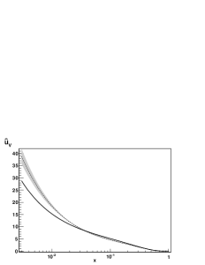
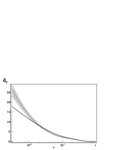
Improved MSTW2008 LO parametrization of ${\hat{q}}_{V}$ obtained via the inverse connection formula (S0.Ex3) is presented in Fig. 1 in comparison with the original MSTW2008 LO parametrization of ${\hat{q}}_{V}$ . One can see that the improved LO parametrization essentially differs from the respective LO parametrization on ${\hat{q}}_{V}$ obtained in standard way, and the difference is not covered by error band.

To better realize what happens when one performs LO analysis of the data let us perform the numerical experiment and prepare the artificial “ideal” polarized semi-inclusive DIS data on pion production. Namely, we consider as such “pseudo-experimental” input the integrated over cut in $z$ proton and deuteron difference asymmetries $A_{p(d)}^{``exp"}{\bigl{|}}_{Z}$, constructed by substitution of the known NLO parametrizations of $u_{V}$, $d_{V}$, $\Delta u_{V}$, $\Delta d_{V}$ and difference of favored and unfavored pion FFs $D_{1}-D_{2}$ into the theoretical expressions for these asymmetries at NLO (see Eqs. (6-10) in Ref. [12]). Then, we extract $\Delta{\hat{u}}_{V}$ and $\Delta{\hat{d}}_{V}$ at LO using these constructed asymmetries $A_{p(d)}^{``exp"}{\bigl{|}}_{Z}$ as a “pseudo-experimental” input in the LO equations (all notation is just as in Ref. [12])

$$A_{p}^{``exp"}{\bigl{|}}_{Z}(x,Q^{2})=(1+R)\frac{4\Delta{\hat{u}}_{V}-\Delta{\hat{d}}_{V}}{4{\hat{u}}_{V}-{\hat{d}}_{V}},\,\,A_{d}^{``exp"}{\bigl{|}}_{Z}(x,Q^{2})=(1+R)(1-\frac{3}{2}\omega_{D})\frac{\Delta{\hat{u}}_{V}+\Delta{\hat{d}}_{V}}{{\hat{u}}_{V}+{\hat{d}}_{V}},$$ (6)

i.e., we perform the LO analysis analogous to one of COMPASS [13], but with the replacement of the real data on $A_{p(d)}^{exp}{\bigl{|}}_{Z}$ by the prepared pseudo-data on $A_{p,(d)}^{``exp"}{\bigl{|}}_{Z}$. The obvious advantage of the latter is that they exist in the widest range in $Q^{2}$, up to $10^{6}\text{ GeV}^{2}$ in accordance with the upper $Q^{2}$ boundary for parametrizations which we use for the pseudo-data preparation. Making use of this advantage we can now comprehensively investigate the influence of $Q^{2}$ on the produced with Eqs. (6) LO results. Namely, we now have a possibility to obtain and compare the LO result on $\Delta{\hat{q}}_{V}$ at the same reference scale ($Q_{ref}^{2}=10\text{ GeV}^{2}$ here) with and without involving the dangerous data at small and moderate $Q^{2}$ into the analysis.

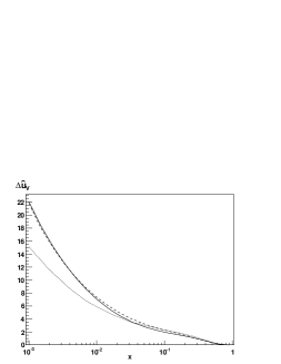
The respective results on $\Delta{\hat{u}}_{V}$ are presented in Figs. 2 and 3 (the results on $\Delta{\hat{d}}_{V}$ are analogous), where, besides the modern parametrization DSSV of $\Delta q$ (Fig. 3), we use also older GRSV parametrization as an input in Eqs. (6) (Fig. 2), because the latter has the LO version, which is useful for comparison.

Dashed line in Fig. 2 corresponds to the original GRSV LO parametrization, while solid and dotted lines in Figs. 2, 3 correspond to direct extraction of $\Delta{\hat{q}}_{V}$ with Eqs. (6) (direct solution of the system (6) with respect to $\Delta{\hat{u}}_{V}$ and $\Delta{\hat{d}}_{V}$), where asymmetries $A_{p,(d)}^{``exp"}{\bigl{|}}_{Z}$ are calculated substituting GRSV NLO (Fig. 2) or DSSV NLO (Fig. 3) parametrizations of polarized PDFs, MSTW2008 NLO parametrization of unpolarized PDFs, and AKK parametrization of FFs into the respective NLO equations (Eqs. (6-10) in Ref. [12]). At the same time, very important difference between $\Delta{\hat{q}}_{V}$ presented by solid and dotted curves is that the first is obtained with asymmetries $A_{p,(d)}^{``exp"}{\bigl{|}}_{Z}$ in Eqs. (6) taken directly at $Q_{ref}^{2}=10\text{ GeV}^{2}$ , while the second is obtained with asymmetries $A_{p,(d)}^{``exp"}{\bigl{|}}_{Z}$ taken at extremely high $Q^{2}=10^{6}\text{ GeV}^{2}$ and only then are evolved to the reference scale $Q_{ref}^{2}=10\text{ GeV}^{2}$. Besides, of importance is that instead of the original MSTW2008 LO parametrization of ${\hat{q}}_{V}$ used for construction of solid lines in Figs. 2 and 3, the respective improved LO parametrization (given by bold solid lines in Fig. 1) is used in denominators of Eqs. (6) for construction of the dotted lines. Indeed, it is clear that to produce the completely corrected (improved) LO results on $\Delta{\hat{q}}_{V}$ one should completely exclude the influence of small $Q^{2}$ on the analysis with Eq. (6). To this end it is not sufficient to restrict the pseudo-data in l.h.s. of Eqs. (6) by the high $Q^{2}$ values and one should also properly correct/improve the denominators in Eqs. (6).

Comparing solid and dashed curves in Fig. 2 one can see that they are very close to each other, which is not surprising, since the vast majority of data used for production of the original GRSV LO parametrization (as well as for production of any other known parametrization) correspond to small and moderate $Q^{2}$ values close to $10\text{ GeV}^{2}$. In contrast, both of these curves in Fig. 2, as well as solid line in Fig. 3 strongly differ from the respective dotted lines, corresponding to the “pure” LO results on $\Delta{\hat{q}}_{V}(10\text{ GeV}^{2},x)$, which are free from the involvement of small $Q^{2}$ data in the analysis.

We will see now that these “pure” LO results (which within the standard approach could be obtained only completely excluding small and moderate $Q^{2}$ data from the analysis) can be reproduced by using the connection formula between LO and NLO QCD orders.

Thus, let us apply the inverse of Eq. (S0.Ex1) connection formula

$$\Delta{\hat{q}}_{V}(Q^{2},x)=\left[\delta(1-x)-\frac{\alpha_{s}(Q^{2})}{2\pi}\left(\frac{\beta_{1}}{\beta_{0}^{2}}\Delta P^{(0)}(x)-\frac{2}{\beta_{0}}\Delta P^{(1)}(x)\right)\right]$$

$$\otimes\;{\rm Exp}\left(\frac{2}{\beta_{0}}\ln\frac{\alpha_{s}(Q^{2})}{{\hat{\alpha}}_{s}(Q^{2})}\,\Delta P^{(0)}(x)\right)\otimes\Delta q_{V}(Q^{2},x),$$ (7)

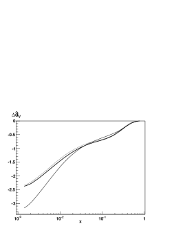
written in terms of the valence helicity PDFs. Substituting in r.h.s. of (S0.Ex4) the modern DSSV NLO parametrization of $\Delta{q}_{V}$ (used for production of Fig. 3) taken at the reference scale $Q^{2}_{ref}=10\text{ GeV}^{2}$ we obtain the respective LO results on $\Delta{\hat{q}}_{V}$ at the same $Q^{2}_{ref}$. The results on $\Delta{\hat{q}}_{V}(10\text{ GeV}^{2},x)$ obtained in this way are presented in Fig. 4 by the bold solid lines and are compared with the respective results, obtained earlier by the use of Eqs. (6) and presented in Fig. 3. Comparing dotted and bold solid lines one can see that while they strongly differ from the thin solid line directly obtained via Eq. (6) at small $Q^{2}_{ref}=10\text{ GeV}^{2}$, they are in excellent agreement with each other. Moreover, they practically merge with each other. Thus, one can conclude that to reach improved LO valence PDFs there is no need to restrict the analysis to use of data produced only at extremely high $Q^{2}$ values (that is hardly possible in reality): the inverse connection formulas give the direct access to the same improved LO PDFs without any additional restrictions on the $Q^{2}$ range from which the data comes. In contrast, the standard procedure of LO analysis can produce these improved PDFs (FFs) at LO only from data in very high $Q^{2}$ region and only after that they should be evolved with DGLAP to the lower $Q^{2}$ values. However, regretfully, the most of statistics is available just at small and moderate $Q^{2}$, so that the such a way of action is realizable in our simple model but seems to be hardly possible in reality.

Let us now briefly discuss some aspects of application of the results on improved PDFs at LO. From this point of view of especial importance is the considered above unpolarized case (see Fig. 1), because unpolarized parton densities enter the denominators of all asymmetries studied nowadays, and, in particular, of the asymmetries giving access to such important and attracting today the great attention PDFs as transverse momentum distributions (TMDs), for which only LO analysis is still possible (see [3, 4] and references therein). Notice, that even in this case there is a good possibility to partially (and significantly) improve LO results on these quantities without knowledge of the respective NLO results as an input in the connection formulas. Such improvement can be achieved by performing the standard LO analysis of the respective measured asymmetries, but using in their denominators the improved unpolarized PDFs at LO instead of the usual LO parametrizations.

Let us see how large can be impact on the LO results only due to improvement of the denominators in the asymmetries analysed at LO in standard way at small $Q^{2}$ values. To this end we return to the considered above numerical experiment based on application of Eqs. (6) and derive the “partially improved” results on LO valence helicity PDFs $\Delta{\hat{q}}_{V}(10\text{ GeV}^{2},x)$ solving the system (6) at $Q^{2}_{ref}=10\text{ GeV}^{2}$ with the improved LO parametrization on $q_{V}$ (bold solid lines in Fig. 1) in denominators instead of the original LO parametrization.

The results on “partially improved” $\Delta{\hat{u}}_{V}$ (long-dashed line) are presented in Fig. 5 in comparison with the respective “naive” (thin solid line, the same as in Figs. 3, 4 ) and “completely improved” (bold solid line, the same as in Fig. 4) LO results. One can see that impact of the “partial improvement” on $\Delta{\hat{u}}_{V}$ is very significant, and the respective curve is even much closer to the line corresponding to the “completely improved” LO results. The picture for $\Delta{\hat{d}}_{V}$ and for application of GRSV NLO parametrization in l.h.s. of Eq.(6) is absolutely analogous.

Thus, one can hope that even in the cases when the state of art still does not allow to extract PDFs/FFs from the data at NLO (for instance, the TMDs case), it is possible, nevertheless, to significantly improve the respective LO results only due to application of the improved LO unpolarized PDFs in denominators of the asymmetries analyzed at LO in standard way.

In summary, the non singlet (inverse) connection formulas (S0.Ex3), (S0.Ex4) between LO and NLO QCD orders were applied to both unpolarized and polarized valence PDFs. It was shown that the connection formulas produce improved LO results on valence PDFs without exclusion from the analysis the data coming from the small and moderate $Q^{2}$ region (only the standard cut $Q^{2}>1\text{ GeV}^{2}$ should be applied). The respective improved LO parametrizations on the valence PDFs were obtained (bold solid lines in Figs. 1, 4), and they strongly differ from the respective original LO parametrizations, obtained by using the most of data produced at small and moderate $Q^{2}$ values. Of importance is the argued statement that within the standard procedures of LO analysis (LO theoretical expressions are applied to the measured asymmetries and cross sections) the same improved LO results could be obtained by using only the data produced at extremely high $Q^{2}$ values, that is hardly possible in reality. It was argued that even in the cases when the state of art still does not allow to extract PDFs/FFs from the data at NLO (for instance, the TMDs case), it is possible, nevertheless, to significantly improve the respective LO results only due to application of the improved LO unpolarized PDFs in denominators of the asymmetries analyzed at LO in the standard way.

Figure 1: Results on ${\hat{u}}_{V}$ (left) and ${\hat{d}}_{V}$ (right) versus $x$ at $Q_{ref}^{2}=10\text{ GeV}^{2}$. The dashed line is MSTW2008 LO parametrization [8]. the gray area is the corresponding error band. The bold solid line corresponds to improved MSTW2008LO parametrization of ${\hat{u}}_{V}$ and ${\hat{d}}_{V}$, which is obtained by using the MSTW2008 NLO parametrization in r.h.s. of inverse connection formula Eq. (S0.Ex3)

Figure 2: $\Delta{\hat{u}}_{V}$ at $Q_{ref}^{2}=10\text{ GeV}^{2}$ versus $x$. Dashed line corresponds to the original GRSV LO parametrization. Solid line corresponds to direct solution of the system (6) with respect to $\Delta{\hat{q}}_{V}$, where asymmetries $A_{p,(d)}^{``exp"}{\bigl{|}}_{Z}$ are taken at $Q_{ref}^{2}=10\text{ GeV}^{2}$ and MSTW2008 LO parametrization of ${\hat{q}}_{V}$ is used in denominators. Asymmetries $A_{p,(d)}^{``exp"}{\bigl{|}}_{Z}$ are calculated substituting GRSV NLO parametrization of polarized PDFs, MSTW2008 NLO parametrization of unpolarized PDFs, and AKK parametrization of FFs into the respective NLO equations (Eqs. (6-10) in Ref. [12]). Dotted line corresponds to $\Delta{\hat{q}}_{V}$ which are obtained in the same way but at extremely high $Q^{2}=10^{6}\text{ GeV}^{2}$ and with improved MSTW2008 LO parametrization of ${\hat{q}}_{V}$ (bold solid lines in Fig. 1) in denominators of Eqs. (6). The obtained in this way ${\hat{q}}_{V}$ are then evolved via DGLAP equations from $Q^{2}=10^{6}\text{ GeV}^{2}$ to $Q_{ref}^{2}=10\text{ GeV}^{2}$.

Figure 3: $\Delta{\hat{u}}_{V}$ at $Q_{ref}^{2}=10\text{ GeV}^{2}$ versus $x$. Solid line corresponds to direct solution of the system (6) with respect to $\Delta{\hat{q}}_{V}$, where asymmetries $A_{p,(d)}^{``exp"}{\bigl{|}}_{Z}$ are taken at $Q_{ref}^{2}=10\text{ GeV}^{2}$ and MSTW2008 LO parametrization on ${\hat{q}}_{V}$ is used in denominators. Asymmetries $A_{p,(d)}^{``exp"}{\bigl{|}}_{Z}$ are calculated substituting DSSV NLO parametrization of polarized PDFs, MSTW2008 NLO parametrization of unpolarized PDFs, and AKK parametrization of FFs into the respective NLO equations (Eqs. (6-10) in Ref. [12]). Dotted line corresponds to $\Delta{\hat{q}}_{V}$ which are obtained in the same way but at extremely high $Q^{2}=10^{6}\text{ GeV}^{2}$ and with improved MSTW2008 LO parametrization of ${\hat{q}}_{V}$ (bold solid lines in Fig. 1) in denominators of Eqs. (6). The obtained in this way ${\hat{q}}_{V}$ are then evolved via DGLAP equations from $Q^{2}=10^{6}\text{ GeV}^{2}$ to $Q_{ref}^{2}=10\text{ GeV}^{2}$.

Figure 4: LO valence helicity PDFs $\Delta{\hat{u}}_{v}$ (left) and $\Delta{\hat{d}}_{v}$ (right) at $Q_{ref}^{2}=10\text{ GeV}^{2}$ obtained in different ways. Bold solid line corresponds to improved LO parametrization, which is obtained from DSSV NLO parametrization via inverse connection formula (S0.Ex4). Thin solid and dotted lines are just the same as in Fig. 3.

Figure 5: $\Delta{\hat{u}}_{V}$ at $Q_{ref}^{2}=10\text{ GeV}^{2}$ versus $x$. Bold solid line corresponds to improved LO parametrizations on $\Delta{\hat{q}}_{V}$, which is obtained from DSSV NLO parametrization via inverse connection formula (S0.Ex4). Thin solid line corresponds to direct solution of the system (6) with respect to $\Delta{\hat{q}}_{V}$, where asymmetries $A_{p,(d)}^{``exp"}{\bigl{|}}_{Z}$ are taken at $Q_{ref}^{2}=10\text{ GeV}^{2}$ and MSTW2008 LO parametrization on ${\hat{q}}_{V}$ is used in denominators. Asymmetries $A_{p,(d)}^{``exp"}{\bigl{|}}_{Z}$ are calculated substituting DSSV NLO parametrization of polarized PDFs, MSTW2008 NLO parametrization of unpolarized PDFs, and AKK parametrization of FFs into the respective NLO equations (Eqs. (6-10) in Ref. [12]). Long-dashed line (“partially improved” LO result on $\Delta{\hat{q}}_{V}$) is obtained in the same way, but with the application of the improved MSTW2008 LO parametrization of ${\hat{q}}_{V}$ (bold solid lines in Fig. 1) in denominators of (6) instead of the original MSTW2008 LO parametrization.

References

- [1] M. Alekseev et al. [COMPASS Collaboration], Phys. Lett. B 693 (2010) 227.
- [2] A. Airapetian et al. [HERMES Collaboration], Phys. Rev. D 87 (2013) 074029
- [3] M. Anselmino, M. Boglione and S. Melis, Phys. Rev. D 86 (2012) 014028
- [4] M. Anselmino, M. Boglione, U. D’Alesio, A. Kotzinian, S. Melis, F. Murgia, A. Prokudin and C. Turk, Eur. Phys. J. A 39, 89 (2009)
- [5] O. Yu. Shevchenko, Phys. Rev. D87 (2013) 114004.
- [6] W. Furmanski and R. Petronzio, Phys. Lett. B 97 (1980) 437.
- [7] W. Vogelsang, Phys. Rev. D 54 (1996) 2023.
- [8] A. D. Martin, W. J. Stirling, R. S. Thorne and G. Watt, Eur. Phys. J. C 63 (2009) 189 [arXiv:0901.0002 [hep-ph]].
- [9] D. de Florian, R. Sassot, M. Stratmann and W. Vogelsang, Phys. Rev. D 80 (2009) 034030.
- [10] M. Gluck, E. Reya, M. Stratmann and W. Vogelsang, Phys. Rev. D 63 (2001) 094005.
- [11] S. Albino, B. A. Kniehl and G. Kramer, Nucl. Phys. B 803 (2008) 42.
- [12] O. Y. Shevchenko, R. R. Akhunzyanov and V. Y. Lavrentyev, Eur. Phys. J. C 71 (2011) 1713.
- [13] M. Alekseev et al. [COMPASS Collaboration], Phys. Lett. B 660 (2008) 458.