Thermodynamic model of social influence
on two-dimensional square lattice:
Case for two features
Abstract
We propose a thermodynamic multi-state spin model in order to describe equilibrial behavior of a society. Our model is inspired by the Axelrod model used in social network studies. In the framework of the statistical mechanics language, we analyze phase transitions of our model, in which the spin interaction is interpreted as a mutual communication among individuals forming a society. The thermal fluctuations introduce a noise into the communication, which suppresses long-range correlations. Below a certain phase transition point , large-scale clusters of the individuals, who share a specific dominant property, are formed. The measure of the cluster sizes is an order parameter after spontaneous symmetry breaking. By means of the Corner transfer matrix renormalization group algorithm, we treat our model in the thermodynamic limit and classify the phase transitions with respect to inherent degrees of freedom. Each individual is chosen to possess two independent features and each feature can assume one of traits (e.g. interests). Hence, each individual is described by degrees of freedom. A single first order phase transition is detected in our model if , whereas two distinct continuous phase transitions are found if only. Evaluating the free energy, order parameters, specific heat, and the entanglement von Neumann entropy, we classify the phase transitions in detail. The permanent existence of the ordered phase (the large-scale cluster formation with a non-zero order parameter) is conjectured below a non-zero transition point in the asymptotic regime .
keywords:
Critical point phenomena, Thermodynamic spin models, Axelrod model, Sociophysics1 Introduction
The original Axelrod model [1], despite its simplicity, has been accepted as a model describing social influence with respect to the interaction among individuals [2, 3]. The interacting individuals of the Axelrod model are located on a regular two-dimensional square lattice and are characterized by a set of cultural features, whereas each feature can assume one of the cultural traits. Each feature represents one of the cultural dimension, e.g., language, religion, technology, style of dress, etc. The dynamics of this model runs in two steps repeated as required. In the first step, an agent (representing an individual) and one of his neighbors are selected randomly. In the second step, the probability of interaction is calculated being proportional to the number of shared features. The interaction consists of selecting a feature at random in which the two agents differ, and setting this feature of the neighboring agent to be equal to the corresponding feature of the agent. It might seem that this mechanism leads to homogenization of society. However, it can lead either to a global homogenization (the ordered phase) or to a fragmented state (disordered phase) with coexistence of different homogeneous regions. One of the main results conjectures a critical value separating a monocultural state from the multicultural [4]. Further details of the thermodynamic Axelrod model and the out-of-equilibrium Axelrod model are discussed in Ref. [5].
In this study we consider a classical multi-spin model of a social system treated from the point of view of the statistical mechanics. We focus our attention on behavior of a model of a large society in equilibrium. The society is represented by individuals who mutually interact via communication channels (e.g. sharing interests) with the nearest neighbors only. The society is subject to special rules given by a model of the statistical mechanics we have introduced for this purpose. A noise plays an important role in this study. The noise interferes with the communication channels. If it increases, the communicating individuals get less correlated on larger distances. In this way the noise acts against the formation of larger clusters of the individuals with a particular character, i.e., a set of shared features. In such a cluster, the individuals share a similar social background. The size of the clusters can be quantified by calculations of an appropriate order parameter, correlation length, etc., which are commonly used in the statistical physics. If a phase transition point exists in a given statistical model, this point separates an ordered phase from the disordered. The two phases can be determined by the order parameter being non-zero within the ordered phase or zero in the disordered, provided that the system is infinitely (sufficiently) large, and the spontaneous symmetry-breaking mechanism occurred below the transition point. The noise can be also regarded as random perturbations (cultural drift) realized as a spontaneous change in a trait [6] and can play a significant constructive role in the out-of-equilibrium Axelrod model. On the other hand, the effect of the noise for such non-linear dynamical systems is found to be size-dependent [7].
We, therefore, propose a multi-state spin model on the two-dimensional regular square lattice of the infinite size. Each vertex of the lattice contains a multi-state spin variable (being an individual with a certain cultural setting). We define special nearest-neighbor interactions among the spins representing a conditional communication among individuals. The statistical Gibbs distribution introduces thermal fluctuations into our model with a multi-spin Hamiltonian. Here, the temperature can be identified as the noise we introduced above. Imposing a constant magnetic field on given spin states makes the spins align accordingly, which might have had a similar effect as, for instance, the mass media or advertisement. Having calculated the effects of the magnetic field, we observed a typical paramagnetic response in our model only, and no phase transition was observed.
The model describes thermodynamic features of social influence studied by the well-known Axelrod model [1]. Gandica et al. [5] have recently studied such thermodynamics features in the coupled Potts models in one-dimensional lattices, where the phase transition occurs at zero temperature in accord with a thermodynamic one-dimensional interacting multi-state spin system. Our studies go beyond this thermodynamic Axelrod model conjectures since we intend to study phase transitions on social systems at non-zero temperature, where number of the individuals is infinite. Therefore, the spontaneous symmetry-breaking mechanism selects a certain preferred cultural character resulting in a large cluster formation, which is characterized by a non-zero order parameter.
This task is certainly nontrivial since our model has not been known to have an analytical solution. Therefore, we apply the Corner Transfer Matrix Renormalization Group (CTMRG) algorithm [8], which is a powerful numerical tool in the statistical mechanics. The CTMRG calculates all thermodynamic functions to a high accuracy and enables to analyze the phase transitions as well as to control the spontaneous symmetry breaking. The phase transition temperature decreases with increasing number of traits as discussed later. We intend to investigate the asymptotic case in this paper, i.e., the case when the number of the traits of each individual is infinite. Then, we estimate the phase transition point in order to find out whether the ordered phase is permanently present or not. In other words, the phase transition point is found to remain non-zero. Throughout this paper we consider the case of only.
The paper is organized as follows. In Sec. II we define the Hamiltonian of our model, briefly describe CTMRG, and introduce the thermodynamic functions used in the analysis of the phase transition. The Sec. III contains numerical calculations explained in the statistical physics language. In Sec. IV we discuss and interpret our results in terms of the communicating individuals influenced by the presence of the noise.
2 Lattice model and CTMRG algorithm
2.1 Hamiltonian and density matrix
A classical spin lattice model is considered on the regular two-dimensional square lattice, where the nearest-neighbor multi-state spins placed on the lattice vertices interact. Let be a generalized multi-spin with integer degrees of freedom . The subscript indices and denote the position of each lattice vertex, where the spins are placed within the and coordinate system on the underlying lattice, i.e., . We start with the -state clock (vector) model [9] for this purpose with the Hamiltonian
| (1) |
The interaction term acts between the nearest-neighbor vector spins . The summation includes the horizontal and the vertical directions on the square lattice.
Let us generalize the spin clock model so that the interaction term contains a special attribute, i.e., extra spins are added. We, therefore, introduce additional degrees of freedom to each vertex. The Hamiltonian in Eq. (1) can be further modified into the form . The position dependent term describes the spin interactions of the -state clock model controlled by additional -state Potts model -interactions [10]. The total number of the spin degrees of the freedom is on each vertex . We study the simplified case when starting from the case of up to which is still computationally feasible. (In more general case when , we do not expect substantially different physical consequences as those studied in this work.)
Hence, our multi-state spin model contains two -state spins on the same vertex, i.e., and , which are distinguished by the superscripts () and (). It is instructive to introduce a -variable . The Hamiltonian of our model has its final form
| (2) |
noticing that , where
| (3) |
The superscript can take only two values as mentioned above. The Potts-like interaction is represented by a diagonal matrix with the elements on the diagonal.
Thus defined model can also describe conditionally communicating (interacting) individuals of a society. The society is modeled by individuals () and each individual has two distinguished features and . Each feature assumes different values (traits). In particular, an individual positioned on vertex of the square lattice communicates with a nearest neighbor, say , by comparing the spin values of the first feature . This comparison is carried out by means of the -state Potts interaction. If the Potts interaction is non-zero, the individuals communicate via the -state clock interaction of the other feature with . The cosine enables a broader communication spectrum than the Potts term. Since we require symmetry in the Potts-clock conditional communication, we include the other term in the Hamiltonian, which exchanges the role of the features () and () in our model. In particular, the Potts-like communication first compares the feature followed by the cosine term with the feature . (Enabling extra interactions between the two features within each individual and/or the cross-interactions of the two adjacent individuals is to be studied elsewhere.) The total number of all the individuals is considered to be infinite in order to detect and analyze the phase transition when the spontaneous symmetry breaking is present.
In the framework of the statistical mechanics, we investigate a combined -state Potts and -state clock model which is abbreviated as the -state spin model. As an example, one can interpret the case of in the following: the feature can be chosen to represent leisure-time interests while the other feature can involve working duties. In the former case, one could list three properties such as reading books, listening to music, and hiking, whereas the latter feature could consist of manual activities, intellectual activities, and creative activities, as the example. The thermal fluctuations, induced by the thermodynamic temperature of the Gibbs distribution, are meant to describe a noise hindering the communication. The higher the noise, the stronger suppression of the communication is resulted.
We classify the phase transitions of our model by numerical calculation of the partition function
| (4) |
especially, by its derivatives. The sum has to be taken through all multi-spin configurations on the infinite lattice. Here, Boltzmann constant and temperature are denoted by and , respectively. The partition function is evaluated numerically by the CTMRG algorithm [8], which generalizes the Density Matrix Renormalization Group [11] on the two-dimensional classical spin systems. In the CTMRG language, the whole square lattice is divided into four identical quarters (corners of the square shape), the so-called corner transfer matrices, and the renormalization group (RG) transformation projects out all those spin configurations which have the lowest probability selected by a density matrix.
A typical formulation of an observable (an averaged thermodynamic function) obeys the standard expression
| (5) |
where the matrix is introduced being commonly called the reduced density matrix
| (6) |
It is a classical counterpart of the one-dimensional quantum reduced density matrix in DMRG defined for a subsystem in contact with an environment . The reduced density matrix is defined on a line of the spins (forming the subsystem ) between any of the two adjacent corner transfer matrices, whereas all the remaining spins variables form the environment . The configuration sum is taken over all spins within the environment except those of the subsystem . Notice the normalization . Its meaning is the partition function within the classical statistical physics and is normalized to unity.
Our model can be thought of as a system with two non-trivially coupled sub-lattices, where either sub-lattice is composed of the -state variables with the given feature .
2.2 Thermodynamic functions
The Helmholtz free energy per spin site
| (7) |
can be easily evaluated from the partition function by CTMRG. Taking derivatives of the free energy determines other thermodynamic functions used in the classification of the phase transition. Namely, the first derivative with respect to temperature results in the internal energy
| (8) |
which is equivalent to the nearest-neighbor correlation function evaluated on the square lattice for the Potts-like models
| (9) |
The consequent derivative of the internal energy with respect to yields the specific heat
| (10) |
which has a non-analytic (divergent) behavior at a phase transition. Analogously, the first and the second derivatives of the free energy with respect to an external magnetic field results in the magnetization (the order parameter) and the susceptibility, respectively. Another important thermodynamic function to be calculated is the entanglement von Neumann entropy . It follows the standard quantum-mechanical definition
| (11) |
This quantity reflects the correlation effects, which are maximal at the phase transition point.
The order parameter can be equivalently evaluated via the reduced density matrix in Eq. (6) being either non-zero within an ordered spin phase or zero in the disordered. A continuous transition usually leads to the second-order phase transition, and the discontinuous behavior signals the first-order phase transition. However, a detailed analysis of the free energy and other thermodynamic functions is usually necessary to distinguish the order of the phase transition.
Let us define a sub-site order parameter for a given feature
| (12) |
where the sub-site order parameter is measured. For simplicity, we excluded the subscripts from the order parameter notation. Another useful definition of the order parameter, measuring both of the spins at the same vertex, is a complete order parameter
| (13) |
Again, we simplified the expression into . We also extended the definition of the complete order parameter by introducing a -state fixed parameter . This parameter specifies the alignment of towards a reference spin level, where the multi-state spin projections are measured. Unless stated explicitly in the text, we often consider the parameter .
The CTMRG algorithm has been a well-established numerical method for almost two decades and recognized by the physical community as an accurate and reliable numerical method [12, 13]. All of the thermodynamic functions can be calculated to a high accuracy, which is governed by the integer number of the CTMRG/DMRG states kept (the higher the number , the better accuracy is reached [8, 11]). Throughout this work we used , which led to the RG truncation error [11] as small as around the phase transition, otherwise the error reaches the machine precision. Additional increasing of the states kept does not change our results.
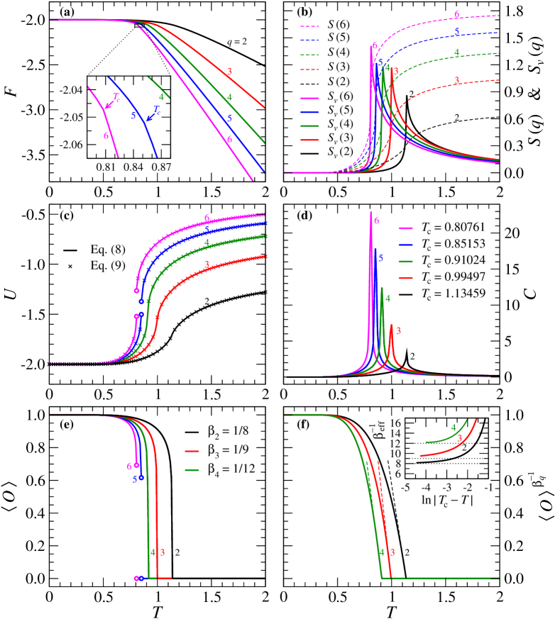
In order to test the efficacy of the CTMRG, we study the standard -state Potts model with a constant magnetic field . The field requires an additional term in the Hamiltonian (2). Since the -state Potts models have analytic expressions for the phase transition temperature , the numerical calculations carried out on this model serves as a benchmark for our model studied later. Figure 1 depicts a couple of selected thermodynamic functions of the -state Potts model for . We calculated the free energy per site in the panel (a). The model exhibits the second order phase transition for . The first order transition is present if , and the free energy has a non-analytic kink as depicted in the inset of the panel (a). The thermodynamic entropy and the von Neumann entanglement entropy , cf. Eq. (11), are shown in the panel (b). The phase transition temperatures correspond to the maxima. The equivalence of the internal energies obtained by Eqs. (8) (full lines) and (9) (the symbols ) are plotted in the panel (c). Here, the discontinuities appearing in are proportional to the non-zero latent heat, which unambiguously confirm the presence of the first order phase transition for and . The divergent peaks of the specific heat in the panel (d) coincide with the phase transition temperatures . The height of the peaks will increase if a finer temperature sampling of is used; each height is limited by the numerical derivatives of the internal energy within the given sampling. The panel (e) shows the complete order parameter remains continuous in the second order transition, but exhibits a discontinuous jump which is typical for the first order phase transition. We also evaluated the critical exponent , which are related to the order parameter . These critical exponents are in agreement with the analytical solutions [10]. The linearity of the order parameter when temperature approaches the critical point from the ordered phase are depicted in the panel (f), where the dashed lines are the tangents at . The inset shows, the convergence of the effective magnetic exponent
| (14) |
where . The horizontal dotted lines serve as guides for the eyes, which correspond to the critical exponents reached in the asymptotic limit .
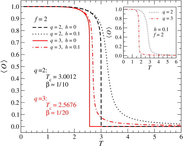
If the magnetic field is set to be non-zero, the thermodynamic functions are always analytic within all temperature range, and no phase transition point is detected. Figure 2 shows this case for and if we applied CTMRG to the model Hamiltonian studied in Ref. [5] on the two-dimensional square lattice. It is evident that for zero field the dashed () and the full () lines exhibit the continuous phase transitions with the critical temperatures and exponents , and , , respectively. Applying the magnetic field , the phase transition is not present, and the model responds in the standard paramagnetic way for (dotted line) and (the dashed-dotted line). Since we are interested in the phase transition analysis of our model, we exclude detailed analysis with non-zero magnetic field in our model.
3 Numerical results
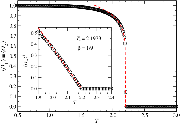
The phase transitions in the classical spin systems are induced by the thermal fluctuations by varying the temperature in Eq. (4). We use dimensionless units, in which . This corresponds to the ferromagnetic spin ordering. We begin with the simplest non-trivial case of . Figure 3 shows the sub-site order parameter with respect to temperature which is identical for both and . The second order phase transition is resulted at the critical temperature . The associated universality scaling results in the common critical exponent . The inset shows nearly linear behavior of when approaching the critical temperature from the ferromagnetic phase. The critical exponent of our model at is very close to the -state Potts model universality class [10], where . This model analogy is non-trivial and requires further clarification. Notice that the exponent differs from the well-known Ising (-state clock) universality, where . It belongs neither to the -state Potts nor -state clock model universality classes.
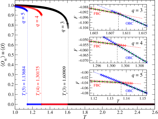
The sub-site order parameter for , , and is depicted in Fig. 4. It gradually decreases with increasing temperature, but at certain temperature it discontinuously jumps to zero. Such behavior usually suggests the first order phase transition. To confirm this statement, the free energy per spin is plotted with respect to for two different boundary conditions (BCs). The fixed (open) BCs are imposed at the very beginning of the iterative CTMRG scheme in order to enhance (suppress) spontaneous symmetry breaking resulting in the ordered (disordered) phase in a small vicinity of the phase transition point. In particular, if the fixed BCs are applied, the spontaneous symmetry-breaking mechanism selects one of free energy minima as specified by the fixed BCs. On the contrary, the open BCs prevent the spontaneous symmetry breaking from falling into a minimum and makes the system be in a metastable state below the phase transition. Since the first-order phase transition is known to exhibit the coexistence of two phases in a small temperature interval around the phase transition, such an analysis with the two different BCs is inevitable to locate the phase transition accurately. The insets for the three cases, , show the normalized Helmholtz free energy around the transition temperature. The red and blue symbols of the free energy correspond to the fixed and the open BCs, respectively. The temperature interval, in which two distinguishable converged free energy are measured according to BCs set, is the region, where the ordered and disordered phases can coexist. The true phase transition point is located at the free energy crossover, and the equilibrium free energy is shown by the thick dashed line corresponding to the lower free energy. In this case, the free energy is a non-analytical at and exhibits a kink typical for the first-order phase transition (further details on the first order analysis are can be found in Ref. [14]). Taking the derivatives of with respect to , a discontinuity of the thermodynamic functions in Eqs. (8) and (10) is resulted. (We remark here that the free energy is not sensitive to the different BCs if a critical second-order phase transition is present, i.e., if .)
The phase transition temperatures for are calculated within a high accuracy resulting , , , and (not plotted) at the crossing point of the free energy. It is obvious that gradually decreases with increasing , and later we study the asymptotic case when . It is also worth to mention that the first-order phase transition is not critical in sense of the non-diverging correlation length at the phase transition temperature (not shown) in contrast to the second order phase transition, when the correlation length diverges. For this reason, we reserve the term critical temperature, , for the second-order phase transition only, which is resulted in our model only if . Otherwise, we use the notation transition temperature .
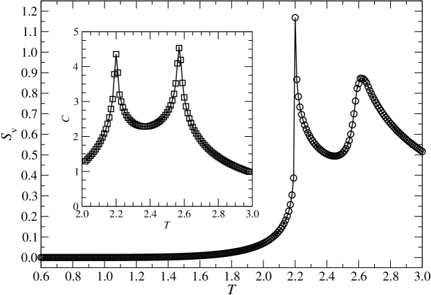
The entanglement von Neumann entropy when is plotted in Fig. 5. Evidently, our calculations of result in two maxima, not only a single maximum as expected for the single phase transition observed in Fig. 3. Hence, the entanglement entropy can indicate the existence of another phase transition, which could not be detected by the sub-site order parameter . The phase transition at lower temperature, , coincides with the one plotted in Fig. 3, whereas the higher-temperature phase transition appears at . To support this result obtained by , we also calculated the specific heat , as shown in the inset. There are two evident maxima in , which remain present in our model at the identical critical temperatures and . The sub-site order parameter in Fig. 3 has not reflected the higher-temperature phase transition at all. Thus, we have achieved a new phase transition point, which is likely pointing to a topological ordering. A second-order transition has been found in the out-of-equilibrium Axelrod model [15]. In addition, the existence of modulated order parameter with two different phase transition temperatures has been reported earlier, often being associated with experimental measurements of the magnetization in crystal alloys [16, 17].
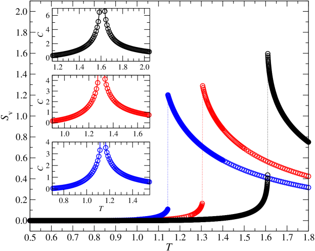
The entanglement entropy exhibits a single maximum for any as seen in Fig. 6. The discontinuity of at the phase transition temperature is characteristic for the first order phase transition. The three insets display the specific heat with the single maximum for each at the transition temperature, which is in full agreement with the sub-site order parameter. Therefore, we conclude the existence of the single phase transition point of the first order if .
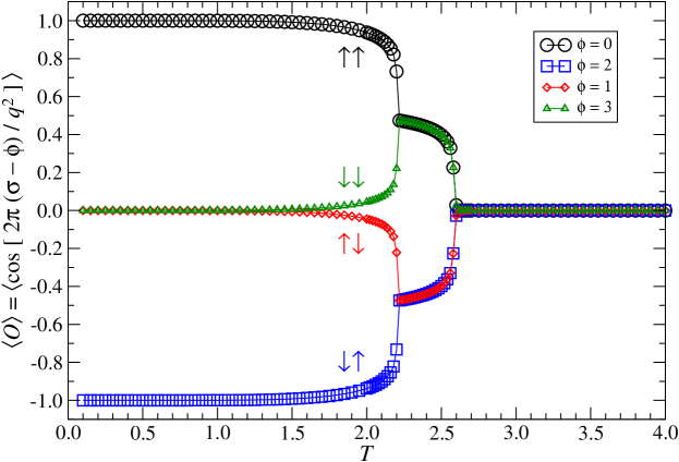
Figure 7 shows the complete order parameter when as defined in Eq. (13). Obviously, the non-analytic behavior of points to the two distinguishable critical temperatures and , which completely coincide with the critical temperatures depicted in Fig. 5. Since the -state spin has four degrees of freedom, by targeting the parameters separately, the complete order parameter is explicitly evaluated. It satisfies the condition that the sum of all four complete order parameters at any temperature has to be zero. The mechanism of the spontaneous symmetry breaking at low temperatures causes that the free energy is four-fold degenerate at most. This is related to the four equivalent free energy minima with respect to the complete order parameter. Accessing any of the four free energy minima is numerically feasible by targeting the reference spin state .
Let us denote the four spin state at the vertex by the notation . There are four possible scenarios for the order parameter as shown in Fig. 7. These scenarios are depicted by the black circles (), the red diamonds (), the blue squares (), and the green triangles (), which correspond to the following vertex configurations , , , and , respectively.
At zero temperature there are three minima of the free energy leading to the three different complete order parameters being , , and . There are four minima of the free energy if so that the order parameter has four different values , , , and with the condition . It means the two states share the same free energy minimum when the order parameter is zero at and . In the temperature interval , there are only two free energy minima present and the order parameter pair for and becomes identical as well as the pair for and . The only single free energy minimum is resulted at when the order parameter is zero, which is typical for the disordered phase.
Let us stress that at the temperatures in between and , the pair of the site configurations and is indistinguishable by the complete order parameter (i.e. the black and green symbols coincide), and the same topological uniformity happens for the pair of the site configurations and . In other words, the anti-parallel alignments between the spins and are preferable in the temperature region .
Notice that if the critical exponent of the complete order parameter is calculated at the critical temperatures and , we found out that if , whereas the other exponent remains identical as discussed earlier, in particular, if .
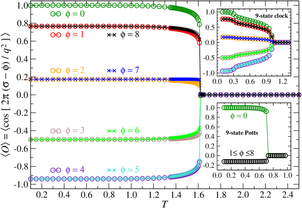
In the same analogy, we plotted the complete order parameter for in Fig. 8. The free energy is five-fold degenerated at zero temperature unless the symmetry breaking mechanism (enhanced by ) selects one of them. This mechanism results in the five distinguishable order parameters within , which decouple into nine different order parameters when . Just a single free energy minimum is characteristic in the disordered phase at exhibiting a uniform . In order to compare the main differences of the complete order parameter between our model and the standard -state clock model or the -state Potts models, we plotted the respective order parameter in the insets of Fig. 8. In the former case (the clock model) there are always five distinguishable order parameters originating in the five-fold degeneracy of the free energy, and the order parameters in our model and the -state clock model are identical at only. However, the five-fold degeneracy remains within the interval . (We remark that the BKT phase transitions [18, 19] of the infinite order is present in the -state clock models [20].) In the latter case (the Potts model), there are only two distinguishable order parameters out of nine below the phase transition point. (Recall that the total sum of over all is always zero. The discontinuity in the complete order parameter at in our model and the -state Potts model reflects the first-order phase transition [10].
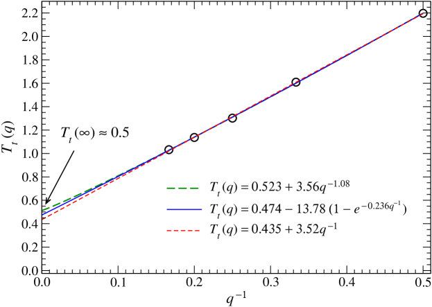
If the number of the spin degrees of freedom is extrapolated toward the asymptotic limit, , a non-zero phase transition temperature is resulted. We carried out the three independent extrapolations as depicted in Fig. 9 by means of the least square fitting. In particular, the power-law , the exponential , and the inverse proportional fitting functions were used to obtain , , and parameters. All of them yielded the non-zero transition temperature . Out of these findings, we conjecture the existence of the ordered phase, i.e., the non-zero phase transition temperature persists for any .
4 Discussion and conclusion
Having been motivated by the Axelrod model, we studied a multi-state thermodynamic spin model we proposed for this purpose. Our model is defined on the two-dimensional infinite square lattice. The spin model is analyzed by the numerical tools of the statistical physics in order to calculate equilibrial properties over a social model. We focused on analyzing phases and the phase transitions. A similar thermodynamic Axelrod model with -state Potts interactions has been first studied analytically by Gandica et al. [5] on one-dimensional chains only. In this case the typical thermodynamic properties of one-dimensional interacting spin systems were concluded with no phase transition, i.e., the phase transition occurs at only. We have reproduced features of the -state Potts model and we have carried out numerical analyses on the identical Hamiltonian of the thermodynamic Axelrod model, as defined in Ref. [5], for and , with the respective non-zero phase transition temperature on the two-dimensional square lattice cf. Fig. 2.
The original out-of-equilibrium Axelrod model in one dimension in the presence of the noise behaves like an ordinary thermodynamic one-dimensional interacting particle system described by the Potts-like Hamiltonian [5]. As demonstrated in Ref. [6], the order-disorder transition induced by the noise depends on the value of , with the dependence becoming weaker for larger values of . In the cited paper, the system tends to homogeneity if the noise is low (because of unstable disordered configurations with respect to the noise perturbations) and vice versa, the system prefers heterogeneity whenever the noise rate gets strong (disappearance of domains is compensated by creating the new ones). We considered the case of in our model, where we have observed a strong -dependence. This affects the phase transition temperature (the critical noise), which decreases with increasing . Moreover, we have provided the thermodynamic analog of the Axelrod model in two dimensions, cf. Fig. 2. In addition, our model does not contain the Potts interactions only, but includes the clock model interactions with a richer communication structure (interaction). Such multi-spin model is again mapped onto mutually communicating individuals subject to a noise, which prevents them in communication. The gradual increase of the noise disables the formation of larger clusters of the individuals who share specific cultural features, e.g., interests (the cluster size is quantified by the order parameter). The raising noise suppresses correlations at longer distances and exhibits the same character as the thermal fluctuations. Each individual is characterized by two independent features (), and each feature assumes different traits (interests) resulting in cultural settings of each individual.
We have found out that such social system exhibits two phase transitions when . Using the above-mentioned examples, one can interpret results in the following: let, for instance, the first feature describe the two activities: ‘reading of books’ () and ‘listening to music’ (), whereas the second two-state feature involves ‘manual activity’ () and ‘intellectual activity’ (). Both of the phase transitions are continuous separating three phases, which are classified into the (i) low-noise regime, (ii) the medium-noise regime, and (iii) the high-noise regime.
(i) In the low-noise regime, the individuals tend to form a single dominant cluster, where the complete order parameter has four values (three if only), see Fig. 7. The statistical probability of forming the dominant clusters is proportional to . If the noise increases and the complete order parameter decreases to the values of , the four different clusters are formed, and a final size of the dominant cluster (chosen be setting the parameter ) decreases proportionally to this complete order parameter. (ii) In the medium-noise regime, an interesting topological regime reveals just two equally likely traits of the individuals. In the social terms, the pairing of the cultural settings coincides either with (1) the equal mixture of those individuals who ‘read books’ and ‘do manual activity’ () and the individuals who ‘listen to music’ and ‘do intellectual activity’ () or (2) the equal mixture of those who ‘listen to music’ and ‘do manual activity’ () and those who ‘read books’ and ‘do intellectual activity’ (). (iii) In the high-noise regime, the clusters are not significant (the correlation length decreases to zero if the noise increases), and the individuals behave in a completely uncorrelated way.
A discontinuous phase transition of the first order is present when the number of the traits . In the low-noise regime, larger clusters of individuals with a given cultural setting (out of ) are formed. The selected cultural setting of the dominant cluster sizes is proportional to the order parameter . This is equivalent to the ordered multi-state spin phase below the phase transition noise . The regime of the uncorrelated individuals (disordered phase) appears above the phase transition noise. The low-noise regime is separated from the high-noise regime by a discontinuity of the cluster size (the complete order parameter).
In the asymptotic limit of the number of the traits (the cultural settings), the extrapolation of the phase transition noise results in the non-zero . We conjecture that the phase transition noise remains finite (being approximately ). We interpret this result as the permanent existence of the correlated clusters below the non-zero phase transition point .
5 Acknowledgments
This work was supported by the grants QIMABOS APVV-0808-12, VEGA-2/0074/12, and EU project SIQS No. 600645.
References
References
- [1] R. Axelrod, The Journal of Conflict Resolution 42 (1997) 203.
- [2] A. Barrat, M. Barthélemy, A. Vespignani, Cambridge University Press (2008).
- [3] C. Castellano, S. Fortunato, V. Loreto, Rev. Mod. Phys. 81 (2009) 591.
- [4] C. Castellano, M. Marsili, A. Vespignani, Phys. Rev. Lett. 85 (2000) 3536.
- [5] Y. Gandica, E. Medina, I. Bonalde, Physica A 392 (2013) 6561.
- [6] K. Klemm, V. M. Eguíluz, R. Toral, and M. S. Miguel, Phys. Rev. E 67 (2010) 045101R.
- [7] R. Toral, and C. J. Tessone, Communications in Computational Physics, 2 (2007) 177.
- [8] T. Nishino, J. Phys. Soc. Jpn. 65 (1996) 891.
- [9] A. Gendiar, R. Krcmar, K. Ueda, and T. Nishino, Phys. Rev. E 77 (2008) 041123.
- [10] F. W. Wu, Rev. Mod. Phys. 54 (1982) 235.
- [11] S. R. White, Phys. Rev. Lett. 69 (1992) 2863.
- [12] U. Schollwöck, Rev. Mod. Phys. 77 (2005) 259.
- [13] U. Schollwöck, Annals of Physics 326, (2011) 96.
- [14] A. Gendiar, T. Nishino, Phys. Rev. E 65 (2002) 046702.
- [15] A. Radillo-Díaz, L. A. Pérez, and M. del Castillo-Mussot, Phys. Rev. E 80 (2009) 066107.
- [16] T. Ito, K. Mizuno, K. Ito, and B. J. Beaudry, J. de Physique C8 (1988) 343.
- [17] T. Sakon, H. Nagashio, K. Sasaki, S. Susuga, D. Numakura, M. Abe, K. Endo, S. Yamashita, H. Nojiri, T. Kanomata, InTech (2013).
- [18] J. M. Kosterlitz and D. J. Thouless, J. Phys. C 6 (1973) 1181.
- [19] J. M. Kosterlitz, J. Phys. C 7 (1974) 1046.
- [20] J. Tobochnik, Phys. Rev. B 26 (1982) 6201.