Do Google Trend data contain more predictability than price returns?

Abstract

Using non-linear machine learning methods and a proper backtest procedure, we critically examine the claim that Google Trends can predict future price returns. We first review the many potential biases that may influence backtests with this kind of data positively, the choice of keywords being by far the greatest culprit. We then argue that the real question is whether such data contain more predictability than price returns themselves: our backtest yields a performance of about 17bps per week which only weakly depends on the kind of data on which predictors are based, i.e. either past price returns or Google Trends data, or both.

1 Introduction

Taking the pulse of society with unprecedented frequency and focus has become possible thanks to the massive flux of data from on-line services. As a consequence, such data have been used to predict the present (Choi and Varian, 2012) (called nowcasting by Castle et al. (2009)), that is, to improve estimates of quantities that are being created but whose figures are to be revealed at the end of a given period. The latter include unemployment, travel and consumer confidence figures (Choi and Varian, 2012), quarterly company earnings (from searches about their salient products) (Da et al., 2011), GDP estimates (Castle et al., 2009) and influenza epidemics (Ginsberg et al., 2008).

The case of asset prices is of particular interest, for obvious reasons. It seems natural that the on-line activity of people who have actually traded is related in some way to contemporaneous price changes. However, forecasting asset price changes with such data is a much harder task. The idea is by no means recent (see e.g. Antweiler and Frank (2004)). The literature investigates the mood of traders in forums devoted to finance (Antweiler and Frank, 2004; Rechenthin et al., 2013), newspapers (Gerow and Keane, 2011), tweets (Bollen et al., 2011), blogs (Gilbert and Karahalios, 2010), or a selection of them (Mao et al., 2011). Determining the mood of traders requires however to parse the content of the posts and to classify them as positive or negative.

A simpler approach consists in using Google Trends (GT thereafter) which reports historical search volume interest (SVI) of chosen keywords and to relate SVIs to financial quantities of interest trading volume, for instance price volatility or price returns (Da et al., 2011; Gerow and Keane, 2011; Wang, 2012; Bordino et al., 2012; Takeda and Wakao, 2013; Preis et al., 2013; Kristoufek, 2013). Findings can be summarized as follows: using this kind of data to predict volume or volatility is relatively easy, but the correlation with future price returns is much weaker. Incidentally, this matches the daily experience of practitioners in finance who use price returns instead of fancy big data.

Here we discuss what can go wrong in every step required to backtest a trading strategy based on GT data. We then use an industry-grade backtest system based on non-linear machine learning methods to show the near-equivalence of the exploitable information content between SVI and historical price returns. We therefore conclude that price returns and GT contain about the same amount of predictive information, at least with the methods we have used and challenge to community to do any better.

2 Backtesting a speculative strategy based on Google Trends data

Price returns are believed to be unpredictable by a sizable fraction of academics. Unconditional raw asset prices are certainly well described by suitable random walks that contain no predictability whatsoever. Our experience as practitioners suggest that predictability is best found conditionally and that linear regressions are not the most efficient tools to uncover non-randomness in this context. There is essentially no linear price return auto-correlation; however some significant cross-correlation are found (in sample) between changes of SVI and future price returns. One would be tempted to conclude that GT data do contain more exploitable information than price returns.

In our opinion, using such methods prevents one to ask the right question and to assess properly the predictability content of either type of data. We propose that one should first build a non-linear prediction algorithm and then feed it with either past returns, GT data, or both, and finally compare the respective performance of each case.

Before reporting such comparisons, we review some dangers associated with the use of GT data for prediction. As the saying goes, prediction is hard, especially about the future. But prediction about the future in the past is even harder because it often seem easier than it should. It is prone to many kinds of biases that may significantly alter its reliability, often positively (Freeman, 1992; Leinweber, 2007). Most of them are due to the regrettable and possibly inevitable tendency of the future to creep into the past. Any small leak from the future may empower an unbiased random strategy into a promising candidate for speculative trading. Let us now look closely at how this happens when trying to find predictability in GT data. The procedure goes as follows:

1. Choose a set of trading strategies

2. Choose the period of backtest

3. Choose a set of assets

4. Choose a set of keywords

5. Download GT data

6. Choose the timescale of returns

7. Choose parameters

8. Compute the performance with predictors consisting of GT data only, price returns only, and both.

The rest of the paper is devoted to discuss each of the above steps.

2.1 Trading strategies

This must be done first, since otherwise one would backtest all kinds of strategies until one stumbles on good-looking strategy.

Academic papers often test and report fixed relationships between an increase of SVI and future price returns. For instance Preis et al. (2013) assume that an increase in SVI with respect to its moving average should be followed by a negative return. The same kind of strategies is found in Kristoufek (2013) who proposes to build a portfolio whose asset weights decrease as a function of their respective SVI. All this is unsatisfactory. There is no reason indeed why a given relationship should hold for the whole period (they do not, see below) and for all stocks. For instance it is easy to find two assets with consistently opposite reactions to SVI changes.

Linear strategies are out for the reasons exposed above. One is then faced with the problem of choosing a family of strategies that will not overfit the input: there may be many keyword SVIs and functions thereof as inputs. We choose therefore to use ensemble learning as a tool to relate different kinds of information and to avoid in-sample overfitting as much possible. Note, however, that this is only one layer of stock selection and investment decision in the backtest system that one of us has implemented.

2.2 Period of backtest

The propensity of academic papers to either stop or start their investigations in 2008, even those written in 2011 (Gerow and Keane, 2011), is intriguing. Kristoufek (2013) uses the whole available length and clearly shows that the relationship between SVI and future returns has dramatically changed in 2008. What this means is that one must properly backtest a strategy with sliding in and out of sample windows (Leinweber, 2007). Computer power used to be an issue, but the advent of very cheap cloud computing power has solved it.

2.3 Choice of assets

Most papers are interested in predicting future price returns of a set of assets, for instance the components of some index (e.g. a subset of Russell 3000 (Da et al., 2011), Dow Jones Industrial average (Kristoufek, 2013)), while some focus on predicting the index itself (Preis et al., 2013). We focus here on the components of the S&P 100 index. The reason why one should work with many assets is to profit from the power of the central limit theorem: assuming that one has on average a small edge on each asset price, this edge will become apparent much faster than if one invests in a single asset (e.g. an index) at equal edge.

2.4 Choice of keywords

This is a crucial ingredient and the most likely cause of overfitting because one may introduce information from the future into the past without even noticing it. A distressing number of papers use keywords from the future to backtest strategies, for instance Preis et al. (2013); Choi and Varian (2012); Janetzko (2014). One gross error is to think of the keywords that could have been relevant in the recent past, for instance debt, AIG, crisis, etc. instead of trying to think of ones which will be relevant. But a much more subtle error is common: to take a set of keywords that is vague enough and eternally related to finance, for instance finance, and to find related keywords with Google Sets (Preis et al., 2013; Choi and Varian, 2012). This service suggests a collection of keywords related to a given set of keywords and is accessible in a spreadsheet from docs.google.com. We entered a single keyword, finance, and asked for related keywords. We did not obtain any fancy keywords (restaurant, color, cancer, etc.) as in Preis et al. (2013), but did find the celebrated keyword debt, among others. The problem is that one cannot ask Google Sets in 2014 what was related to finance in 2004. As a consequence, the output of Google Sets introduces information from the future into a backtest. Since, as far as we know, Google Sets does not provide a wayback machine, it must not be used at all to augment one’s set of keywords used to backtest a strategy. This shows that the choice of keywords is a crucial ingredient.

In addition, the use of Google was not stationary during the whole period, which may introduce significant biases into the backtest results. Correcting them needs at least a null hypothesis, i.e. a null set of keywords known before the start of the backtest period. This is why we collected GT data for 200 common medical conditions/ailments/illnesses, 100 classic cars and 100 all-time best arcade games that we trust were known before 2004 (cf. appendix A) and applied the strategy described in Preis et al. (2013) with $k=10$. Table 1 reports the t-statistics (t-stats henceforth) of the best three positive and negative performances (the latter can be made positive by inverting the prescription of the strategy, transaction costs permitting) for each set of keywords, including the one from Preis et al. (2013).

Ailments	t-stat
multiple sclerosis	-2.1
muscle cramps	-1.9
premenstrual syndrome	-1.8
alopecia	2.2
gout	2.2
bone cancer	2.4

Classic cars	t-stat
Chevrolet Impala	-1.9
Triumph 2000	-1.9
Jaguar E-type	-1.7
Iso Grifo	1.7
Alfa Romeo Spider	1.7
Shelby GT 500	2.4

Classic arcade games	t-stat
Moon Buggy	-2.1
Bubbles	-2.0
Rampage	-1.7
Street Fighter	2.3
Crystal Castles	2.4
Moon Patrol	2.7

Preis et al. (2013)	t-tstat
labor	-1.5
housing	-1.2
success	-1.2
bonds	1.9
Nasdaq	2.0
investment	2.0

Table 1: Keywords and associated t-stats of the performance of a simple strategy using Google Trends time series to predict SPY from Monday close to Friday close prices. Transaction costs set at 2bps

Our brain is hard-wired to make sense of noise and is very good at inferring false causality. We let the reader ponder about what (s)he would have concluded if bone cancer or Moon Patrol were more finance-related. This table also illustrates that the best t-stats associated to the keyword set of Preis et al. (2013) are not significantly different from what one would obtain by chance: the t-stats reported here being a mostly equivalent to Gaussian variables for time series longer than, say, 20, one expects 5% of their absolute values to be larger that 1.95. One notes that debt is not among the three best keywords when applied to SPY from Monday to Friday: its performance is unremarkable and unstable, as shown in more details below. This issue is discussed in more details in challet2013predicting.

2.5 Google Trends data

Google Trends data are biased in two ways. First, GT data were not reliably available before 6 August 2008, being updated randomly every few months (Wikipedia, 2013). Backtests at previous dates include an inevitable part of science fiction, but are still useful to calibrate strategies.

The second problem is that these data are constantly being revised, for several reasons. The type of data that GT returns was tweaked in 2012. It used to be made of real numbers whose normalization was not completely transparent; it also gave uncertainties on these numbers. Quite consistently, the numbers themselves would change within the given error bars every time one would download data for the same keyword. Nowadays, GT returns integer numbers between 0 and 100, 100 being the maximum of the time-series and 0 its minimum; small changes of GT data are therefore hidden by the rounding process (but precision is about 5% anyway) and error bars are no more available. This format change is very significant: for instance, the process of rounding final decimals of prices sometimes introduces spurious predictability, which is well known for FX data (Johnson, 2005). In the case of GT data, any new maximum increases the granularity of the data, thereby making it even less reliable. It is one of the reasons members of quantopedian.com could not replicate the results of (Preis et al., 2013) before the GT data set was released by the authors (Cuantopian.com, 2014). This problem can be partly solved by downloading data for smaller overlapping time periods and joining the resulting time series.

2.6 Price returns resolution

GT data have a weekly resolution by default; most academic papers make do with such coarse resolution. Note that one downloads them trimester by trimester, GT data have a daily resolution. As a somewhat logic consequence, they try to predict weekly price returns. In our experience, this is very ambitious and predictability will emerge more easily if one times one’s investment, if only for instance because of day-of-the-week effect (Gibbons and Hess, 1981).

2.7 Parameter tuning

Most trading strategies have tunable parameters. Each set of parameters, which include keywords, defines one or more trading strategies. Trying to optimize parameters or keywords is equivalent to data snooping and is bound to lead to unsatisfactory out-of-sample performance. When backtest results are presented, it is often impossible for the reader to know if the results suffer from data snooping. A simple remedy is not to touch a fraction of historical data when testing strategies and then using it to assess the consistence of its performance, but only once (cross-validation) (Freeman, 1992). More sophisticated remedies include White’s reality check (White, 2000) (see e.g. Sullivan et al. (1999) for an application of this method). Data snooping is equivalent to having no out-of-sample, even when backtests are properly done with sliding in- and out-of-sample periods.

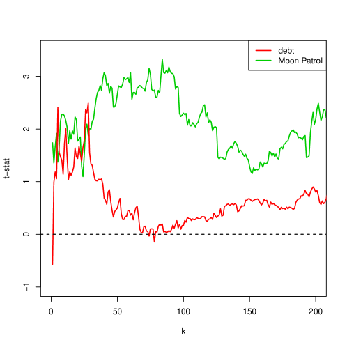
Let us perform some in-sample parameter tuning on the strategy proposed in Preis et al. (2013). Figure 1 reports the t-stat of the performance associated with the keyword debt as a function of $k$, the length of the reference simple moving average. Its sign is relatively robust against changes over the range of $k\in{2,\cdots,30}$ but its typical value in this interval is not particularly exceptional. Let us take now the absolute best keyword from the four sets, Moon Patrol. Both the values and stability range of its t-stat are much better than those of debt (see Figure 1), but this is entirely due to pure chance.

Figure 1: T-stats of the performance associated with keywords debt and Moon Patrol versus the length of the moving average $k$. Transaction costs set to 2bps per transaction.

Figure 2: Cumulated performance associated with the four sets of keywords. Each transaction costs 2bps.

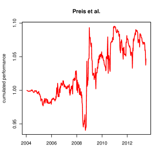
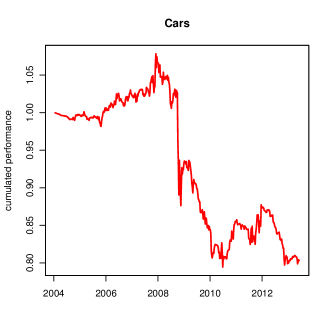
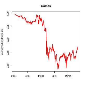
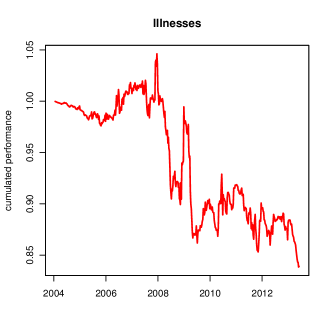
One solution to avoid parameter overfitting is to average the performance of a strategy over a reasonable range of parameters. Let us take $k=1,\cdots,100$ for each keyword of each list introduced above. Since all the keywords act on a single asset, we use for each list an equally weighted scheme and hence compute the mean position over all keywords and all $k$s. The resulting cumulated performance net of transaction costs set at 2bps per transaction (which subtracts about 15% to the performance computed over the period considered) is reported in Fig. 2. It is rather random for random keywords but slightly positive for the biased keywords of Preis et al. (2013), which is consistent with the overall positive bias of t-stats that they report. It is however not very appealing, with an annualized zero-interest rate Sharpe ratio of about 0.12 and a t-stat of 0.37, which are far from being significant. In addition, its performance is flat from 2011 onwards, i.e. out of sample.

2.8 Compare price returns and GT data as predictors

Figure 3: Cumulated performance, net and gross exposures, and number of stocks in the portfolio for both GT and returns (left), only GT (middle) and only price returns (right). Each transaction costs 2bps.

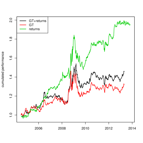
	weekly return [bps]	weekly volatility [bps]	annualized IR	t-stat
GT+returns	17.1	134	0.92	2.73
returns	16.9	133	0.92	2.72
GT	18.3	134	0.99	2.93

Table 2: Summary statistics of backtested performance for the three types of predictors.. Each transaction costs 2bps.

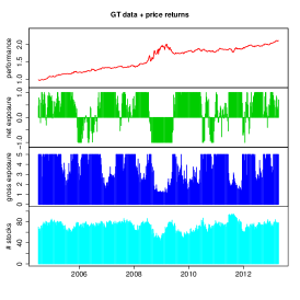
We follow the good idea to choose as keywords company tickers and names (see e.g. Da et al. (2011); Kristoufek (2013)) but add also other simple, non-overfitting, keywords of our own invention. Weekly GT data has been downloaded on 2013-04-21. At first, we do not attempt to predict pure weekly returns but time the investment period. Feeding our backtest system with GT data and returns yields the leftmost plot of Figure 3: there is some exploitable information in these data. Calibration window length is about 6 months, which appears in 2008 and 2009 when the system first learns to take short positions only and then reverts to long positions. This takes much time and shows the difficulty one is faced with when calibrating trading strategies with weekly signals. Summary statistics are reported in Table 2. It is important to be aware that these backtests are much affected by tool bias, as they use heavy computational methods and powerful computers that were not available for most of the backtest period.

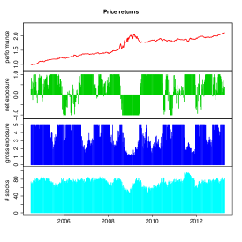
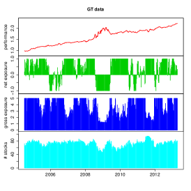
Let us now compare the performance of predictors based on GT data only or past returns only (Fig. 3). We find essentially the same performance (see Table 2); the value of the Wilcox rank sum test p-value is 0.72: they are not very different. This may be due to the fact that the backtest system just learns to recognize trends unconditionally, in other words, that the predictors are simply equally useless. We therefore remove some information content from the predictors. This is done for example by computing a rolling median of each predictor; a value of the predictor is now reduced to a binary number which encodes which side of the previous median it belongs to. We then use exactly the same backtesting system as before with the same parameters. The performance associated to GT data and price returns is now unambiguous (Fig. 4). The machine learning method used here could exploit less predictability from GT inputs (at least those we could think of) than from inputs based on price returns; however, other machine learning methods yield the opposite result.

Figure 4: Cumulated performance both GT and returns, GT only, and returns only when using binary inputs. Same parameters as Fig. 3. Transaction costs set at 2bps.

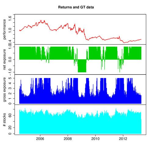
Finally, Figure 5 reports the result of the same method applied on weekly returns, which shows how hard prediction may be in this case even without transaction costs.

Figure 5: Cumulated performance, net and gross exposures, and number of stocks in the portfolio for both GT and returns. Positions may be changed at the market close of each Monday. No transaction costs.

3 Discussion

We have not been able to show that Google Trends data contain more exploitable information than price returns themselves. Assuming that this is not due to us not using the right method, our findings suggest that Google Trends data are equivalent to price return themselves. They do share indeed many properties with price returns: they are aggregate signals created by many individuals, they reflect something related to the underlying assets. In addition both are very noisy: the uncertainty about GT data, gathered from their previous file format, is about 5%. From this point of view, there is nothing miraculous or ground-breaking about GT data.

We had to use sophisticated non-linear methods coupled with a careful backtest procedure, which contrasts with the much simpler approaches usually seen in current academic literature. Why it was needed at all is probably because it is hard to guess at first what an increase in SVI means, since it may be related to good news (e.g. higher interest from potential customers), or bad ones (e.g. worry about the company itself), or both, or neither. Indeed, such data include too many searches unrelated to the financial assets for a given keyword, and even many more unrelated to actual trading. As a consequence, adding another signal based on the change of the number of news related to a given asset helps to interpret what a change of SVI means (Wang, 2012; Cahan, 2012). Another possibility is to use other sources of data, such as Twitter or Wikipedia (Moat et al., 2013), which have the invaluable advantage of being available at a much higher frequency. At any rate, we challenge the community to show that for a given backtest system, predictors based on weekly Google Trends data only are able to outperform predictors based on price that themselves yield about 17bps per week including 2bps transaction costs.

We acknowledge stimulating discussions with Frédéric Abergel, Marouanne Anane (Ecole Centrale) and Thierry Bochud (Encelade Capital).

Appendix A Keywords

We have downloaded GT data for the following keywords, without any manual editing.

A.1 Illnesses

Source:http://www.ranker.com/list/list-of-common-diseases-most-common-illnesses/diseases-and-medications-info, accessed on 27 May 2013
AIDS, Acne, Acute bronchitis, Allergy, Alopecia, Altitude sickness, Alzheimer’s disease, Andropause, Anorexia nervosa, Antisocial personality disorder, Arthritis, Asperger syndrome, Asthma, Attention deficit hyperactivity disorder, Autism, Avoidant personality disorder, Back pain, Bad Breath, Bedwetting, Benign prostatic hyperplasia, Bipolar disorder, Bladder cancer, Bleeding, Body dysmorphic disorder, Bone cancer, Borderline personality disorder, Bovine spongiform encephalopathy, Brain Cancer, Brain tumor, Breast cancer, Burns, Bursitis, Cancer, Canker Sores, Carpal tunnel syndrome, Cervical cancer, Cholesterol, Chronic Childhood Arthritis, Chronic Obstructive Pulmonary Disease, Coeliac disease, Colorectal cancer, Conjunctivitis, Cradle cap, Crohn’s disease, Dandruff, Deep vein thrombosis, Dehydration, Dependent personality disorder, Depression, Diabetes mellitus, Diabetes mellitus type 1, Diaper rash, Diarrhea, Disabilities, Dissociative identity disorder, Diverticulitis, Down syndrome, Drug abuse, Dysfunctional uterine bleeding, Dyslexia, Ear Infections, Ear Problems, Eating Disorders, Eczema, Edwards syndrome, Endometriosis, Epilepsy, Erectile dysfunction, Eye Problems, Fibromyalgia, Flu, Fracture, Freckle, Gallbladder Diseases, Gallstone, Gastroesophageal reflux disease, Generalized Anxiety Disorder, Genital wart, Glomerulonephritis, Gonorrhoea, Gout, Gum Diseases, Gynecomastia, HIV, Head Lice, Headache, Hearing impairment, Heart Disease, Heart failure, Heartburn, Heat Stroke, Heel Pain, Hemorrhoid, Hepatitis, Herniated Discs, Herpes simplex, Hiatus hernia, Histrionic personality disorder, Hyperglycemia, Hyperkalemia, Hypertension, Hyperthyroidism, Hypothyroidism, Infectious Diseases, Infectious mononucleosis, Infertility, Influenza, Iron deficiency anemia, Irritable Male Syndrome, Irritable bowel syndrome, Itching, Joint Pain, Juvenile Diabetes, Kidney Disease, Kidney stone, Leukemia, Liver tumour, Lung cancer, Malaria, Melena, Memory Loss, Menopause, Mesothelioma, Migraine, Miscarriage, Mucus In Stool, Multiple sclerosis, Muscle Cramps, Muscle Fatigue, Muscle Pain, Myocardial infarction, Nail Biting, Narcissistic personality disorder, Neck Pain, Obesity, Obsessive-compulsive disorder, Osteoarthritis, Osteomyelitis, Osteoporosis, Ovarian cancer, Pain, Panic attack, Paranoid personality disorder, Parkinson’s disease, Penis Enlargement, Peptic ulcer, Peripheral artery occlusive disease, Personality disorder, Pervasive developmental disorder, Peyronie’s disease, Phobia, Pneumonia, Poliomyelitis, Polycystic ovary syndrome, Post-nasal drip, Post-traumatic stress disorder, Premature birth, Premenstrual syndrome, Propecia, Prostate cancer, Psoriasis, Reactive attachment disorder, Renal failure, Restless legs syndrome, Rheumatic fever, Rheumatoid arthritis, Rosacea, Rotator Cuff, Scabies, Scars, Schizoid personality disorder, Schizophrenia, Sciatica, Severe acute respiratory syndrome, Sexually transmitted disease, Sinusitis, Skin Eruptions, Skin cancer, Sleep disorder, Smallpox, Snoring, Social anxiety disorder, Staph infection, Stomach cancer, Strep throat, Sudden infant death syndrome, Sunburn, Syphilis, Systemic lupus erythematosus, Tennis elbow, Termination Of Pregnancy, Testicular cancer, Tinea, Tooth Decay, Traumatic brain injury, Tuberculosis, Ulcers, Urinary tract infection, Urticaria, Varicose veins.

A.2 Classic cars

Source:http://www.ranker.com/crowdranked-list/the-best-1960_s-cars, accessed on 27 May 2013
1960 Aston Martin DB4 Zagato, 1960 Ford, 1961 Ferrari 250 SWB, 1961 Ferrari 250GT California, 1963 Corvette, 1963 Iso Griffo A3L, 1964 Ferrari 250 GTL (Lusso), 1965 Bizzarrini 5300 Strada, 1965 Ford GT40, 1965 Maserati Mistral, 1965 Shelby Cobra, 1966 Ferrari 365P, 1966 Maserati Ghibli, 1967 Alfa Romeo Stradale, 1967 Ferrari 275 GTB/4, 1967 Shelby Mustang KR500, 1968 Chevrolet Corvette L88, 1968 DeTomaso Mangusta, 1969 Pontiac Trans Am, 1969 Yenko Chevelle, 57 Chevy, 68 Ferrari 365 GTB/4Daytona Spyder, 69 Yenko Camaro Z28, AC Cobra, Alfa Romeo Spider, Aston Martin DB5, Austin Mini Saloon 1959, BMW E9, Buick Riviera, Buick Wildcat, Cane, Chevrolet Camaro, Chevrolet Chevelle, Chevrolet Impala, Chevy Chevelle, Chrysler Valiant, Corvette Stingray, Dodge Challenger, Dodge Charger, Dodge Dart Swinger, Facel Vega Facel II, Ferrari 250, Ferrari 250 GTO, Ferrari 250 GTO, Ferrari 275, Ferrari Daytona, Fiat 500, Ford Corsair, Ford Cortina, Ford GT40, Ford Mustang, Ford Ranchero, Ford Thunderbird, Ford Torino, Ford Zephyr MK III, Iso Grifo, Jaguar E-type, Jeep CJ, Lamborghini Miura, Lamborghini Miura SV, Lincoln Continental, Lotus Elan, Maserati Ghibli, Mercedes Benz 220SE, Mercedes-Benz 300SL, Mercury Cougar, Plymouth Barracuda, Pontiac GTO, Porsche 356, Porsche 911, Porsche 911, Porsche 911 classic, Rambler Classic, Rover 2000, Shelby Daytona Coupe, Shelby GT350, Shelby GT500, Studebaker Avanti, Sunbeam Tiger, Toyota 2000GT, Triumph 2000, Vauxhall Velox 1960, Vauxhall Victor 1963, Wolseley 15/60

A.3 Arcade Games

Source:http://www.ranker.com/list/list-of-common-diseases-most-common-illnesses/diseases-and-medications-info, accessed on 27 May 2013
1942, 1943, 720°, After Burner, Airwolf, Altered Beast, Arkanoid, Asteroids, Bad Dudes Vs. DragonNinja, Bagman, Battlezone, Beamrider, Berzerk, Bionic Commando, Bomb Jack, Breakout, Bubble Bobble, Bubbles, BurgerTime, Centipede, Circus Charlie, Commando, Crystal Castles, Cyberball, Dangar - Ufo Robo, Defender, Dig Dug, Donkey Kong, Donkey Kong 3, Donkey Kong Junior, Double Dragon, Dragon’s Lair, E.T. (Atari 2600), Elevator Action, Final Fight, Flashback, Food Fight, Frogger, Front Line, Galaga, Galaxian, Gauntlet, Geometry Wars, Gorf, Gorf, Gyruss, Hogan’s Alley, Ikari Warriors, Joust, Kangaroo, Karate Champ, Kid Icarus, Lode Runner, Lunar Lander, Manic Miner, Mappy, Marble Madness, Mario Bros., Millipede, Miner 2049er, Missile Command, Moon Buggy, Moon Patrol, Ms. Pac-Man, Naughty Boy, Pac-Man, Paperboy, Pengo, Pitfall!, Pole Position, Pong, Popeye, Punch-Out!!, Q*bert, Rampage, Red Baron, Robotron: 2084, Rygar: The Legendary Adventure, Sewer Sam, Snow Bros, Space Invaders, Spy Hunter, Star Wars, Stargate, Street Fighter, Super Pac-Man, Tempest, Tetris, The Adventures of Robby Roto!, The Simpsons, Time Pilot, ToeJam & Earl, Toki, Track & Field, Tron, Wizard Of Wor, Xevious

References

- Antweiler and Frank [2004] Werner Antweiler and Murray Z Frank. Is all that talk just noise? the information content of internet stock message boards. The Journal of Finance, 59(3):1259–1294, 2004.
- Bollen et al. [2011] Johan Bollen, Huina Mao, and Xiaojun Zeng. Twitter mood predicts the stock market. Journal of Computational Science, 2(1):1–8, 2011.
- Bordino et al. [2012] Ilaria Bordino, Stefano Battiston, Guido Caldarelli, Matthieu Cristelli, Antti Ukkonen, and Ingmar Weber. Web search queries can predict stock market volumes. PloS one, 7(7):e40014, 2012.
- Cahan [2012] Rochester Cahan. Quant 3.0 – harnessing the mood of the web, 2012. URL http://qwafafew.org/images/uploads/DBQQWAFAFEW201212.pdf. [Online; accessed 16-July-2013].
- Castle et al. [2009] Jennifer L Castle, Nicholas WP Fawcett, and David F Hendry. Nowcasting is not just contemporaneous forecasting. National Institute Economic Review, 210(1):71–89, 2009.
- Choi and Varian [2012] Hyunyoung Choi and Hal Varian. Predicting the present with Google Trends. Economic Record, 88(s1):2–9, 2012.
- Cuantopian.com [2014] Cuantopian.com. Google search terms predict market movements, 2014. URL https://www.quantopian.com/posts/google-search-terms-predict-market-movements. [Online; accessed 5-March-2014].
- Da et al. [2011] Zhi Da, Joseph Engelberg, and Pengjie Gao. In search of attention. The Journal of Finance, 66(5):1461–1499, 2011.
- Freeman [1992] John D Freeman. Behind the smoke and mirrors: Gauging the integrity of investment simulations. Financial Analysts Journal, pages 26–31, 1992.
- Gerow and Keane [2011] Aaron Gerow and Mark T Keane. Mining the web for the voice of the herd to track stock market bubbles. In Proceedings of the Twenty-Second international joint conference on Artificial Intelligence-Volume Volume Three, pages 2244–2249. AAAI Press, 2011.
- Gibbons and Hess [1981] Michael R Gibbons and Patrick Hess. Day of the week effects and asset returns. Journal of business, 54(4):579, 1981.
- Gilbert and Karahalios [2010] Eric Gilbert and Karrie Karahalios. Widespread worry and the stock market. In ICWSM, pages 59–65, 2010.
- Ginsberg et al. [2008] Jeremy Ginsberg, Matthew H Mohebbi, Rajan S Patel, Lynnette Brammer, Mark S Smolinski, and Larry Brilliant. Detecting influenza epidemics using search engine query data. Nature, 457(7232):1012–1014, 2008.
- Janetzko [2014] Dietmar Janetzko. Using twitter to model the eur/usd exchange rate. arXiv preprint arXiv:1402.1624, 2014.
- Johnson [2005] N. F. Johnson, 2005. private communication.
- Kristoufek [2013] Ladislav Kristoufek. Can google trends search queries contribute to risk diversification? Scientific reports, 3, 2013.
- Leinweber [2007] David J Leinweber. Stupid data miner tricks: overfitting the S&P 500. The Journal of Investing, 16(1):15–22, 2007.
- Mao et al. [2011] Huina Mao, Scott Counts, and Johan Bollen. Predicting financial markets: Comparing survey, news, twitter and search engine data. arXiv preprint arXiv:1112.1051, 2011.
- Moat et al. [2013] Helen Susannah Moat, Chester Curme, Adam Avakian, Dror Y Kenett, H Eugene Stanley, and Tobias Preis. Quantifying Wikipedia usage patterns before stock market moves. Scientific reports, 3, 2013.
- Preis et al. [2013] Tobias Preis, Helen Susannah Moat, and H Eugene Stanley. Quantifying trading behavior in financial markets using Google Trends. Scientific reports, 3, 2013.
- Rechenthin et al. [2013] Michael Rechenthin, W Nick Street, and Padmini Srinivasan. Stock chatter: Using stock sentiment to predict price direction. Algorithmic Finance, 2(3):169–196, 2013.
- Sullivan et al. [1999] Ryan Sullivan, Allan Timmermann, and Halbert White. Data-snooping, technical trading rule performance, and the bootstrap. The Journal of Finance, 54(5):1647–1691, 1999.
- Takeda and Wakao [2013] Fumiko Takeda and Takumi Wakao. Google search intensity and its relationship with returns and trading volume of japanese stocks. 2013.
- Wang [2012] Yanbo Wang. Media and google: The impact of supply and demand for information on stock returns. Available at SSRN 2180409, 2012.
- White [2000] Halbert White. A reality check for data snooping. Econometrica, 68(5):1097–1126, 2000.
- Wikipedia [2013] Wikipedia. Google trends – Wikipedia, The Free Encyclopedia, 2013. URL http://en.wikipedia.org/wiki/Google_Trends. [Online; accessed 4-June-2013].