SCoPE: An efficient method of Cosmological Parameter Estimation

Abstract:

Markov Chain Monte Carlo (MCMC) sampler is widely used for cosmological parameter estimation from CMB and other data. However, due to the intrinsic serial nature of the MCMC sampler, convergence is often very slow. Here we present a fast and independently written Monte Carlo method for cosmological parameter estimation named as Slick Cosmological Parameter Estimator (SCoPE), that employs delayed rejection to increase the acceptance rate of a chain, and pre-fetching that helps an individual chain to run on parallel CPUs. An inter-chain covariance update is also incorporated to prevent clustering of the chains allowing faster and better mixing of the chains. We use an adaptive method for covariance calculation to calculate and update the covariance automatically as the chains progress. Our analysis shows that the acceptance probability of each step in SCoPE is more than $95\%$ and the convergence of the chains are faster. Using SCoPE, we carry out some cosmological parameter estimations with different cosmological models using WMAP-9 and Planck results. One of the current research interests in cosmology is quantifying the nature of dark energy. We analyze the cosmological parameters from two illustrative commonly used parameterisations of dark energy models. We also asses primordial helium fraction in the universe can be constrained by the present CMB data from WMAP-9 and Planck. The results from our MCMC analysis on the one hand helps us to understand the workability of the SCoPE better, on the other hand it provides a completely independent estimation of cosmological parameters from WMAP-9 and Planck data.

1 Introduction

Precision measurements in the cosmological experiments have improved dramatically in the past few decades. Several ground based and space based high precision cosmological experiments have been undertaken and many other future experiments have been proposed. After WMAP-9 and Planck data release, an ample amount of data is now available in the hands of cosmologists. The goal of cosmologists is to extract the maximum amount of information from these data in about the different cosmological parameters. Thus, techniques for robust and efficient estimation of cosmological parameters is one of the most important tools needed in the cosmologist’s arsenal.

Markov Chain Monte-Carlo (MCMC) methods are widely used to sample the multi-dimensional space of the parameters and estimate the best-fit parameters from the cosmological dataset. One of the most widely used MCMC algorithm for sampling the posterior is Metropolis-Hastings (MH) sampler [1, 2, 3, 4]. However, MH samplers typically require several thousands of model evolutions and only a fraction of them get accepted. Hence, it is challenging to apply the algorithm to problems where the model evaluation is computationally time consuming. Also due to the intrinsic serial nature of the MH chains, it often takes long time to map the posterior. Therefore, even if the multi-processor parallel compute clusters are available they are not utilized efficiently. In this paper, we present an efficient implementation of the MCMC algorithm, dubbed, SCoPE (Slick Cosmological Parameter Estimator), where an individual chain can also be run in parallel on multiple processors.

Another major drawback of the MH method is the choice of step-size. If the step-size in not chosen properly then the rejection rate increases and the progress of the individual chain becomes slower. The step size of the MCMC method is chosen using trial and error method. However, for the cases where the model evolutions are computationally time consuming, such as in cosmology, this type of trial and error method is computationaly uneconomical. Therefore, several authors have proposed different statistical methods for choosing the optimum step-size. An adaptive proposal Monte Carlo method is proposed by Haario et al.[5] that uses the history of the chains to predict the next movement of the chains to improve the acceptance of the steps. The concept of inter-chain adaptation has been proposed in [6]. Several other theoretical proposals for choosing the optimal step size are also available in literature [7].

There are several codes available for cosmological parameter estimation. Publicly available CosmoMC [2, 4], AnalizeThis [9] codes are MCMC code, widely used for posterior mapping of the cosmological parameters. There are other codes such as CosmoPSO [10], CosmoHammer [11] which can find the optimum cosmological parameters very fast, however they failed to sample the posterior fairly. Hence, the statistical quantities (mean, variance and covariance etc.) derived from the sample cannot readily yield unbiased estimates of the population mean, variance etc. Also CosmoMC uses the local MH algorithm [9], fairly samples the posterior only asymptotically, i.e. practically for ’sufficiently’ long run. Hence, if the samples runs are not long enough the posteriors may not get sampled fairly. In this work we devise and implement methodological modifications to the MCMC technique that lead to better acceptance rate. The algorithm proposed in this paper is a standard global MCMC algorithm combined with

• A delayed rejection method that allows us to increase the acceptance rate.

• Pre-fetching is incorporated to make the individual chains faster by computing the likelihood ahead of time.

• An adaptive inter-chain covariance update is also added to allow the step-sizes to automatically adapt to the optimum value.

As a demonstration, we use SCoPE to carry out parameter estimation in different cosmological models including the ‘standard’ 6-parameter $\Lambda$CDM model. There are many reasons to explore well beyond the simple 6-parameter $\Lambda$CDM model. Comprehensive comparison calls for an ability to undertake efficient estimation of cosmological parameters, both owing to increase parameters or the increased computational expense for each sample evolution. For example recent data from WMAP-9 and Planck comfirm that the power at the low multipoles of the CMB angular power spectrum is lower than that predicted in the best-fit standard $\Lambda$CDM model and unlikely to cause by some observational artefact. This has motivated the study of broader class of inflationary models that have infra-red cutoff or lead to related desired features in the primordial power spectrum [12, 13]. Another interesting cause for this power deficiency at the low multipoles can be the ISW effect in a modified the expansion history of the universe [15]. Then, it is important to check if any scenerio in the vast space of dark energy models provides a better fit to the observational data[14]. In this paper, we analyze as illustration, two standard dark energy models $\--$ The first one is the constant equation of state dark energy model [2, 16, 17] with constant sound speed. The second one is the CPL dark energy parametrization proposed in [18, 19] with a linearly varying equation of state. Our analysis shows that both the dark energy models provide marginally better fits to the data than the standard $\Lambda$CDM model.

Another important subject in cosmology is the primordial Helium abundance, denoted by $Y_{He}$. A number of researchers have attempted to pin down the Helium fraction using different data sets. Though the primordial Helium abundance does not directly affect the perturbations spectrum, it affects the recombination and re-ionization processes and consequently changes the CMB power spectrum. The theoretical prediction of primordial Helium abundance from the standard Big Bang nucleosysthesis (BBN) is $Y_{He}\thickapprox 0.24$ [20, 21]. We have carried out the parameter estimation for $Y_{He}$ together with other standard $\Lambda$CDM cosmological parameters to asses the constraint from current CMB data and check if the allowed range is consistent with the BBN prediction.Our analysis shows that the data from WMAP-9 and Planck can put a fairly tight constraint on the cosmological Helium fraction, which matches with the theoretical BBN value.

SCoPE is a C code written completely independently from scratch. The mixing of multiple chains in SCoPE is better and convergence is achieved faster. The paper is organized as follows. The second section provides a brief overview of the standard Metropolis Hastings algorithm. In the third section, we discuss the modifications to the MCMC algorithm incorporated in SCoPE to make it more efficient and economical. In the fourth section of the paper, we provide illustrative results from our analysis of different cosmological models with WMAP-9 and Planck data. Our work also provides a complete independent parameter estimation analysis of the data using an independent MCMC code. The final section is devoted to conclusions and discussions.

2 Brief overview of Metropolis-Hastings algorithm

The Metropolis-Hastings (MH) is one of the most widely used MCMC sampler, in which the posterior i.e. $\pi(\theta)$ is sampled using a random walk. A standard Markov Chain at each step $i$, randomly chooses a candidate value $\theta_{i+1}$ from the proposal distribution $q(.|\theta_{i})$. The candidate value only depends on the current data point $\theta_{i}.$ The new data point is then accepted with probability $\alpha=\min(1,\pi(\theta_{i+1})/\pi(\theta_{i}))$. If the new data point rejected, the previous point is replicated by increasing its weight by $+1$. The chain of data-points thus generated, approximate the target posterior distribution $\pi(\theta)$.

The proposal distribution is generally taken to be a Gaussian distribution i.e. $q(\theta_{i+1}|\theta_{i})$ $=N\exp(-\frac{s}{2}u_{i}(C^{ij})^{-1}u_{j})$, where $u_{i}=\theta_{i+1}-\theta_{i}$ and $C^{ij}$ is the covariance matrix. $s$ is the step size. Theoretical optimum step size for an ideal distribution that provide the best acceptance rate is $s=2.4/\sqrt{n}$ for a $n$ dimensional MCMC sampler [8]. The covariance matrix is provided as an input to the program. As the exact covariance matrix is unknown before the analysis, in practice an approximate covariance matrix, often based on some previous analysis, is provided. If no prior information is available about the covariance between parameters then some approximate diagonal matrix is also often used. However, in such cases the acceptance rate of the sampler may reduce drastically and can be ensured to remain reasonable only by trial and error. Therefore, a better choice is to start with a initial guess diagonal covariance matrix and then to update the covariance matrix using the data points obtained so far from the chain [9]. This requires no prior knowledge about parameter covariance.

Parallelization of MH sampler is generally done by running multiple chains. Whether it is better to run a longer chain than running multiple short chains has been addressed and argued by many authors [22, 23]. But, for running multiple parallel chains proper mixing between the chains has to be ensured. Therefore, each of the multiple chains has to be long enough so that the it can represent an unbiased sample of the population. Gelman-Rubin “$R$” statistics [24] is generally used for testing the mixing of chains. For convergence, the chains have to be long enough such that $R$ is very close to unity. For practical purposes it is taken as $R<1.2$. However, this criterion is often not sufficient for ensuring proper sampling.

In SCoPE multiple chains are used because running a single long chain in serial is computationally time consuming and hence is not feasible for extensive problems of cosmological parameter estimation. Hence, it is desirable to devise an implementation of MH algorithm that allows the individual chains to run in parallel and increase the acceptance rate of the models of a chain. Apart from that the mixing of the chains are also necessary. The next section describes the modifications made to standard MH algorithm to accomplish effective parallelization through prefetching together with all other above mentioned features, namely, enhanced acceptance, regular covariance update from samples, as described in next section.

3 Embellishing the standard Metropolis-Hastings algorithm

3.1 Prefetching

The MCMC can take advantage of parallel computing only by running number of distinct individual chains each on separate processors as shown in [25]. However, the drawback of this method is that the error related to the burn in steps will be present in all the chains. Hence, the initial steps from all the chains need to be removed, which leads to a huge wastage of computational power. In certain problems, the time spent in the burn-in phase may be significant if the convergence rate of the chains is slow. More importantly, if the individual chains are not long enough then they may not pick up the samples from same distribution due to clustering within individual chains. Hence, the poor mixing of the chains is another major concern. Apart from that a small chain may not sample the tail part of the posterior adequately. Therefore, it is extremely useful to speed up the generation of a single chain, through parallelization rather than using multiple chains. When the state-space of the chain is high dimensional, one possible way to do this is to divide the state-space into blocks, and then handle each block on a separate processor for each iteration of the Markov chain. This approach does indeed speed up generation of a single chain, but requires additional effort, in carrying out detailed analysis of the limiting distribution, in order to determine the appropriate blocks. This may be difficult or even impossible in many cases, where the conditional dependence structure in the limiting distribution is complicated. Therefore, in our work we make the individual chains parallel by precomputing several draws from the posterior distribution ahead of time via multiple evolution of models simultaneously in parallel and then use only the values that are needed [25].

Figure 1: Prefetching scheme is explained in the text with the help of above figure

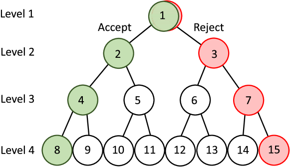
Prefetching is a draw level parallelization in a single chain [26, 27]. The method can be explained by taking the binary tree of a Metropolis algorithm as shown in Fig. 1. In a $k^{th}$ level binary tree there are total $2^{k}-1$ nodes, each of which represents a possible future state of a metropolis algorithm. The branches at the left child of any node represent the accepted steps and the right child represents the rejected states. If we have enough computational resources then all $2^{k}-1$ nodes can be evaluated simultaneously and $k$ steps of a MCMC chain can be carried out in parallel simultaneously.

Though the method of prefetching allows to parallelize a single chain, it only uses $k$ steps out of $2^{k}-1$ computations. The rest of the computations are not utilized. Therefore, many argue against computing all the nodes of the binary tree. Rather if we know the acceptance rate at a point of time from the previously accepted data points, we can statistically identify and precompute only the most probable chain and hence avoid any unnecessary wastage of computation power. It is easy to see that if the acceptance probability at any point of time is less than $0.5$ then the extreme right chain (1-3-7-15-..) of Fig. 1 will be most probable chain. In a similar manner if the acceptance rate is more than $0.5$ then the extreme left chain (1-2-4-8-..) will be the most probable chain. Therefore, by pre-evoluting only the most probable chain, we parallelize the code and at the same time we can manage the computational resources in a better way. Hence, we have adapted this technique in SCoPE.

3.2 Delayed rejection

Delayed rejection is a concept proposed by A. Mira [28, 29, 30, 31, 32, 33]. One of the major problems with the MCMC method is the choice of the step size for the proposal distribution. If the step size is large then rejection rate increases because the variation of the likelihood from sample to sample will be very large. On the other hand if the step-size is taken to be very small then the convergence will be very slow and the auto-correlation between samples will increase. So it is important to choose the step-size optimally. The optimal step-size can be chosen by trial and error method or by some other statistical method, which we discuss in a later section. But even if we choose some optimal step size for the proposal distribution, the acceptance rate may not be very high. It will be better if the rejected sample from one step can be used to determine the proposal distribution for the next sample. This increases acceptance rate but at a cost of violation of the Markovian property. But if we can find some method that can change the acceptance probability of the sample point to compensate the step size variation then that will be useful.

The concept of delayed rejection can briefly be explained as follows. Suppose at some step $i$, the position of a chain is $\theta_{i}=x$. Suppose at this time a candidate $y_{1}$ is accepted from $q_{1}(x,y_{1})$ and accepted with probability

$$\alpha_{1}(x,y_{1})=\min\left(1,\frac{\pi(y_{1})q_{1}(y_{1},x)}{\pi(x)q_{1}(x,y_{1})}\right)$$ (1)

as in the standard MH algorithm. For a Markov chain, $q_{1}(y_{1},x)$ is time symmetric, i.e. $q_{1}(y_{1},x)=q_{1}(x,y_{1})$. Therefore, the acceptance ratio only depends on the posterior. A rejection at any step suggests that there is a local bad fit of the correct proposal and a better one, $q_{2}(x,y_{1},y_{2})$, can be constructed in light of this. But, in order to maintain the same stationary distribution the acceptance probability of the new candidate, $y_{2}$, has to be properly computed. A possible way to reach this goal is to impose detailed balance separately at each stage and derive the acceptance probability that preserves it. A Mira in [28] has shown that if the acceptance probability is taken as

$$\alpha_{2}(x,y_{1},y_{2})=\min\left(1,\frac{\pi(y_{2})q_{1}(y_{2},y_{1})q_{2}(y_{2},y_{1},x)\left[1-\alpha_{1}(y_{2},y_{1})\right]}{\pi(x)q_{1}(x,y_{1})q_{2}(x,y_{1},y_{2})\left[1-\alpha_{1}(x,y_{1})\right]}\right)\,,$$ (2)

then Markovian property of the chain will not get destroyed, but still the sample choice can be made dependent on the previously accepted data point. This particular procedure gives rise to a Markov chain which is reversible with invariant distribution thus provides an asymptotically unbiased estimate of the posterior distribution.

The delayed rejection method can be continued further, if the second sample also gets rejected. A general acceptance probability for a $N$ step delayed rejection is proposed in [28]. But for our purpose we have just consider a $1$ step delayed rejection algorithm. In our algorithm if a data point at a particular step is rejected then we decrease the step size and sample a new data point. The acceptance probability for the new data point is calculated using Eq(2). This increases the acceptance rate of a chain and decreases the autocorrelation between the data points by keeping the chain in motion instead of getting stuck at some step.

No DR &	DR &	DR &	DR &	DR &	DR &
No PF	No PF	1 PF	2 PF	3 PF	4 PF
24.53%	49.12%	67.37%	84.71%	92.79%	97.37%

Table 1: Acceptance rate of a chain with and without delayed rejection (DR) and pre-fetching (PF) for a particular run of the MCMC code. Counts exclude the samples from the burn in steps.

Table (1) lists the acceptance rate of a chain for a SCoPE run. The acceptance rate in the initial steps of the burn in process is poor as the covariance matrix is not known properly. However, as the covariance matrix gets updated due to the adaptive covariance update, the acceptance rate gradually increases to some fixed value. Therefore, the initial burn in steps are not included in the acceptance rate analysis. Without any delayed rejection and prefetching the normal acceptance rate is as poor as $~{}25\%$. This means most of the steps get replicated several times. There are many steps that get replicated more than 20 times, increasing the autocorrelation of a chain. With delayed rejection the acceptance rate increases to $~{}50\%$. For the pre-fetching the acceptance rate is defined as (Number of accepted data point)/(Number of steps). In a $n$ step pre-fetching we are running $n$ parallel computation in each step. Using only $3$ to $4$ prefetching steps we are able to reach more than $90\%$ acceptance rate.

3.3 Inter-chain covariance adaptation

The practical problem in implementing MH is the tuning problem of the proposal distribution $q$ so that the sampling is efficient. One of the recent improvements in the MCMC efficiency is to introduce adaptive samplers. The adaptive MCMC uses the sample history and automatically tune the proposal distribution in the sampling process e.g.[34, 35, 36, 37]. In adaptive metropolis algorithm [35, 38], the covariance matrix from the samples obtained so far is used as the covariance of a Gaussian proposal. Hence the new candidates are proposed as $\theta_{i+1}\sim N(\theta_{i},\Sigma_{i})$ where $\Sigma_{i}=\rm Cov(\theta_{1,...,}\theta_{i})+\epsilon I$ and $\rm I$ is the identity matrix. The method can be used to make the MCMC algorithm adaptive.

The most common parallelization scheme of MCMC method is to run parallel chains instead of running a single one. If in each chains proposal distribution is adapted using the local covariance matrix then the acceptance probability a chain may improve, however, the inter-chain mixing will not improve. If some chain stuck at some local minima then the local covariance matrix corresponding to that chain will be erroneous. So, in case of a local peak the local covariance update will give covariance corresponding to the local peak. In that case, the mixing of chains will slow down and sampling may not be proper. Therefore, in this paper we have adapted the concept of the inter-chain covariance update in the adaptation technique. We run several parallel chains, and randomly update the covariance matrix taking the data points accepted till then from all the chains. This means we have used the covariance as $\Sigma_{i}=\rm Cov(\theta_{1_{1}}..,\theta_{i_{1},}\theta_{1_{2},..,}\theta_{i_{2}....}\theta_{1_{n}},...,\theta_{i_{n}})$, where, $n$ is the number of chains. This inter-chain covariance adaptation [38] speeds up the mixing of the the chains and covers the sample space faster.

The value of the covariance matrix will freeze after few adaptations and hence we will be using same Gaussian proposal after few steps, which is important to guarantee proper sampling. The inter-chain covariance update speeds up the mixing of the chains and thus the Gelman Rubin statistics converges within very few steps. However, if the adaptive covariance is not frozen, it may give rise to unfair sampling as the Gaussian proposal will vary between steps. Therefore, the process of the adaptive covariance calculation is only used for the initial burn in process and after that the adaptation is stopped, during which the covariance calculation attains partial convergence. The effectiveness of the process can be seen from Fig. 2.

Figure 2: The plots show the value of the parameter $\tau$ for first 175 steps of the accepted MCMC chain on WMAP-9 year data. The top plot shows the five chains from a MCMC run where inter-chain adaptive covariance update is applied and the bottom plot show chains from a run without any covariance update and step-size update. It can be seen that for the case of adaptive covariance and step-size update almost all the chains converge within first 20-30 accepted steps, however when adaptive covariance update is not applied, the chains take really long time to converge (approximately 160 steps). The choice of parameter $\tau$ in above is inconsequential. Similar improvement is seen for any other parameter.

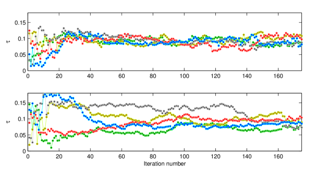
In the Fig. 2 we have shown first 175 values of the quantity $\tau$ for five chains of a MCMC run. It can be seen that when in inter-chain adaptive covariance update is incorporated, the chains converge just after 20-30 steps, which is really fast. Whereas in the case where no inter-chain covariance update is incorporated, the chains take more than 150 steps to attain convergence. Therefore, the burn in steps significantly reduce.

4 WMAP-9 and Planck parameter estimation with SCoPE

In this section we show examples of cosmological parameter estimation with SCoPE using WMAP-9 and Planck data using the likelihood estimators provided by the respective teams. The first example is for the standard 6 parameter $\Lambda$CDM model. Here we have shown a comparative analysis of the WMAP-9 and Planck results.

Standard $\Lambda$CDM model parameter estimation from WMAP-9 and Planck data sets has been carried out by many authors. The 6 main parameters which are used for standard $\Lambda$CDM parameter estimation are physical baryon density ($\Omega_{b}h^{2}$), physical matter density ($\Omega_{m}h^{2}$), Hubble parameter ($h$), reionization optical depth ($\tau$), scalar spectral index ($n_{s}$), amplitude of the temperature fluctuations ($A_{s}$).

Figure 3: Results of cosmological parameter estimation from WMAP-9 (in blue) and Planck (in red) for the standard 6 parametric $\Lambda$CDM model. The lower triangle panels show plots of the $68\%$ and $95\%$ confidence conturs for pairs of parameters. The upper triangle mention the covariance between the pairs parameters. The diagonal plots are the 1 dimensional marginalized distribution of the parameters. The average, standard deviation and the best fit values of these parameters are tabulated below the panels.

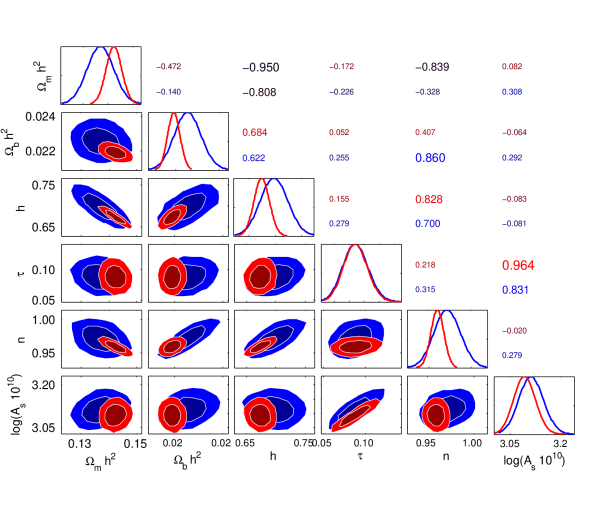
The result from WMAP-9 and Planck simulations are shown in Fig. 3. Likelihoods are calculated using the likelihood software provided by WMAP-9 and Planck team [39, 40]. For calculating the Planck likelihood, we have used low like_v222.clik and CAMspec_v6.2TN_2013_02_26.clik and added them up. We have not used the actspt_2013_01.clik data set as that is only used to obtain constraint very high multipoles of the CMB power spectrum. We have used only the standard 6 parameter model. All the nuisance parameters are fixed to their average values from Planck+WP+highl+BAO parameter estimation as given in [20]. The result of cosmological parameters allowing variation in the nuisance parameters is shown in a later section of the paper.

The result from WMAP-9 and Planck for the standard $6$ parameter model is shown in Fig. 3. It can be seen that the error bars on the parameters decreases substantially for Planck. The results from our analysis matches very well with the results quoted in Planck papers [20]. The small deviations are due to the fact that we have fixed the nuisance parameters their average values. The full analysis result with all the nuisance parameters is shown in a later section.

4.1 Different dark energy parametrization

Recent data from Planck suggest that the power at the low multipoles of the CMB power spectrum is lower than the theoretically expected value. In [14, 15], it is shown the low power at the low multipoles can originate from the ISW effect, which can only affect the CMB low multipoles without introducing any significant features in any other observables. ISW effect comes from the late time expansion history of the universe, which is controlled by the properties of Dark energy in the universe. Therefore, it is important to check if standard variants of dark energy models provide a better fit to the CMB data.

Figure 4: The $68\%$ and $95\%$ confidence contour for the constant equation of state dark energy model. The blue plots are form the WMAP-9 results and the red plots are from Planck results. The dark energy sound speed $c_{s}^{2}$ is almost flat which shows that $c_{s}^{2}$ cannot be constrained using WMAP-9 or Planck results.

Figure 5: One dimensional likelihood plot for the constant equation of state dark energy. Blue plot is showing the WMAP-9 result and the red curve show is for the Planck data.The plots shows that the peak of $\omega$ is very much close to the $-1$ for WMAP-9. However for Planck results the peak has shifted to $\sim-1.2$. The plots shows that $c_{s}^{2}$ cannot be constrained by the data set. The likelihood curve for $c_{s}^{2}$ is almost flat.

Several dark energy models are available in literature such as cosmological constant, quintessence [41, 42, 43], k-essence [44, 45, 46], phantom fields [47], tachyons [48] etc. Different empirical parameterizations for the dark energy are also proposed by authors. Here we have tested some of the standard dark energy models. The generalized equation for a fluid assumption of dark energy perturbation is shown in [14]. There are two parameters for quantifying dark energy perturbations, which are the equation of state $\omega$ and the dark energy sound speed $c_{s}^{2}$. There are models where the $\omega$ is a function of scale factor. We analyze two models and try to fix these parameters using SCoPE.

Figure 6: Plot shows scatter distribution of the samples $\omega_{0}$ vs $\omega_{a}$ plane with the value of $h$ color coded on it. It is clear that $\omega_{0}$ and $\omega_{a}$ are strongly negatively correlated. The black dotted lines shows the $\Lambda$CDM model. The left plot is for WMAP-9 year data set and the right plot is for Planck data set. Though for WMAP-9 data the $\Lambda$CDM model is at the center of the distribution, the Planck data shows slight deviation from the $\Lambda$CDM model. The $\Lambda$CDM model is located at the edge of the distribution for Planck data.

Constant equation of state dark energy model

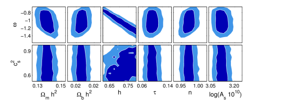
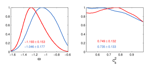
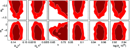
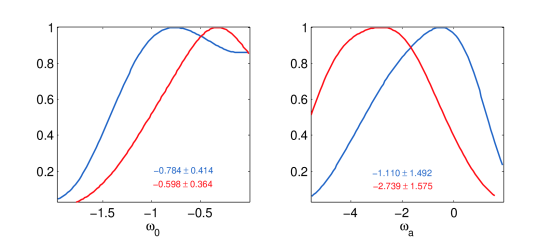
For the constant equation of state dark energy, $\omega$ is constant and hence we need to fix $c_{s}^{2}$ and $\omega$ along with the other 6 standard model cosmological parameters. We run SCoPE for a 8 parameter model. The covariance between the standard model parameters is almost similar to that of the standard model parameters. Therefore, we do not show the plots of those parameters. The $68\%$ and $95\%$ confidence contours of $\omega$ and $c_{s}^{2}$ with other 6 standard model parameters are shown in Fig. 4. It can be seen that the dark energy equation of state is strongly negatively correlated with Hubble parameter. This strong correlation is expected as dark energy equation of state $\omega$ changes the expansion history of the universe that leads to the change in distance of the last scattering surface. This change is actually compensated by the change in Hubble parameter. Apart from $H$, dark energy equation of state is almost uncorrelated with any other standard model parameter. The second row shows that $c_{s}^{2}$ is almost uncorrelated with any other standard model parameters. The data from WMAP-9 or Planck are not good enough to put any constraint on $c_{s}^{2}$. The dark energy sound speed mainly affects the low multipoles of the CMB power spectrum. However, the effect is not strong enough to put any bound on sound speed. In Fig. 5 we show the one dimensional marginal probability for $\omega$, $c_{s}^{2}$. It can be seen that the dark energy equation of state ($\omega$) peaked near $-1$ for WMAP-9, indicating that the standard $\Lambda$CDM model is very good assumption for the dark energy model. Though the peak shifted towards $\omega\sim-1.25$ for the Planck data, which mainly caused by the power deficiency at the low multipoles of $C_{l}^{TT}$. Also, the probability distribution for $c_{s}^{2}$ is almost flat. Therefore, we can conclude that it is almost impossible to put any constraint on $c_{s}^{2}$ using the present CMB data sets.

Figure 7: 2 dimensional likelihood distributions of $\omega_{0}$ and $\omega_{a}$ with other $6$ standard model parameters. The blue plots are for WMAP-9 data and the red plots are for the Planck data. Plots shows that $\omega_{0}$ and $\omega_{a}$ are almost uncorrelated with all the standard model parameters except $h$.

Figure 8: 1-dimensional marginalized probability distributions of $\omega_{0}$ and $\omega_{a}$. Blue curve is for WMAP9 and Red curve is corresponds to Planck data. The plots show that the upper bound on $\omega_{0}$ is not strongly constrained by the data set.

CPL Dark energy parametrization

The CPL dark energy parametrization is an empirical dark energy parametrization, introduced by Chevallier and Polarski [18] and later by Linder [19]. In the CPL dark energy model the equation of state of the dark energy is taken as

$$\omega(a)=\omega_{0}+\omega_{a}(1-a)\,.$$ (3)

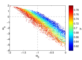
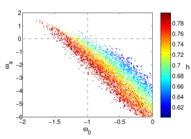
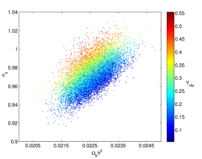
In the analysis we try to estimate $\omega_{0}$ and $\omega_{a}$ along with other $6$ standard model parameters. We have taken the $c_{s}^{2}=1$. In Fig. 6 we have plotted $\omega_{0}$ vs $\omega_{a}$ in the scatter diagram and we have color coded $h$ in it. It can see that there is a negative correlation between $\omega_{0}$ and $\omega_{a}$. In Fig. 7 we have plotted the two dimensional likelihood distributions. It shows that there are strong negative correlation between $\omega_{0}$ and $h$. In Fig. 8 we have shown the one dimensional marginal probability distribution of the dark energy parameters i.e. $\omega_{0}$ and $\omega_{a}$. It can be seen that upper bound on $\omega_{0}$ is not tight. Also the results from WMAP-9 and Planck differ significantly from one another.

Figure 9: Scattered plot of $n_{s}$ vs $\Omega_{b}h^{2}$ color coded with $Y_{He}$. The plots show that if $Y_{He}$ is increased $n_{s}$ increases and $\Omega_{b}h^{2}$ decreases. The left plot is for WMAP-9 year dataset and right plot is for the Planck dataset.

4.2 Helium fraction

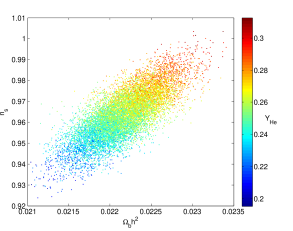
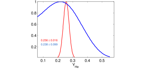
Though the primordial helium fraction, $Y_{He}$ does not affect the CMB perturbations directly, its indirect effect on recombination and reionization can change the CMB power spectrum [20, 21]. For understanding the effects of $Y_{He}$ on the CMB power spectrum we can use the free electron fraction, $f_{e}=n_{e}/n_{b}$, where $n_{e}$ is the free electron number density and $n_{b}$ is the baryon number density. Before HeII recombination ($z>6000$) all the electrons were free and hence free electron fraction was $f_{e}=1-Y_{He}/2$. After HeII recombination the free electron fraction drops down to $f_{e}=1-Y_{He}$, and this remains valid up to redshift $z=1100$. Then hydrogen and HeI recombines and hence $f_{e}$ drops down to almost to values close to zero. Finally, after reionization at late time $f_{e}$ becomes $1-Y_{He}$. Therefore, if $Y_{He}$ is changed then the free electron fraction will change at various epochs. This will lead to the change in recombination and reionization redshift. It may appear that if Helium fraction is changed then to compensate it we can change the baryon fraction in the universe. However, $Y_{He}$ does not change the ratio of the even and odd peaks. Therefore, changing baryon fraction does not actually compensate the features induced from $Y_{He}$. An increase in $Y_{He}$ supress the power of the CMB power spectrum at the high multipoles. Therefore the primordial tilt of $n_{s}$ can compensate $Y_{He}$ up to some extenct. In Fig. 9 we have shown the scatter plot between the scalar spectral index $n_{s}$ and the physical baryon density $\Omega_{b}h^{2}$, and color coded the data points according to the helium fraction i.e. $Y_{He}$. The one dimensional marginalized distribution of primordial helium fraction is shown in Fig. 10, it can be seen that the likelihood peaks close to the standard model helium fraction i.e. $0.24$. Therefore, we can put a very tight constraint on the helium fraction from the observational data from Planck.

Figure 10: Plot shows 1 dimensional marginal probability distribution for $Y_{He}$. Blue plot is for WMAP-9 year data and Red plot is for Planck data. The plots shows that the constrain on $Y_{He}$ highly improved by the Planck observation relative to WMAP.

4.3 SCoPE with full 19 Planck parameters

The results from a simpler standard $6$ parameter model is presented in section(4) with the nuisance parameters fixed to their average value obtained by the Planck collaboration [51]. For testing the code it is important to run SCoPE on a higher dimensional parameter space. In this section we have SCoPE’d the $19$ dimensional parameter space with $6$ standard $\Lambda$CDM parameters and other Planck nuisance parameters. With all 19 parameters the acceptance probability of the sample points is as low as $\sim<1\%$. However, as SCoPE can run the indivudial chains in parallal, the acceptance probability can be increased as much as we want by increasing the number of processors. We have used $10$ CPU for parallelizing each of the chains. and ensure that we take more than $~{}2000$ data points from each of the chain to get a better distribution of the posterior. The results of our analysis are in a good agreement with the Planck collaboration results. We have quoted the average and the best-fit values in Table 2.

Parameter	Definitation	Mean $\pm$ SD	Best fit
$\Omega_{b}h^{2}$	Physical baryon density	0.0220$\pm$0.0003	0.0220
$\Omega_{m}h^{2}$	Physical matter density	0.1421$\pm$0.0028	0.1424
$h$	Hubble parameter	0.6712$\pm$0.0118	0.670
$\tau$	Reion optical depth	0.089$\pm$0.013	0.088
$n_{s}$	Scalar spectral index	0.96$\pm$0.0068	0.961
$\log(10^{10}A_{s})$	Scalar spectral amplitude	3.092$\pm$0.025	3.126
$A_{100}^{PS}$	Contribution of Poisson point-source power to $D_{3000}^{100\times 100}$ for Planck (in $\mu K^{2}$)	183.0$\pm$52.9	159.6
$A_{143}^{PS}$	Same as $A_{100}^{PS}$ but at $143$GHz	56$\pm$11	63.0
$A_{217}^{PS}$	Same as $A_{100}^{PS}$ but at $217$GHz	113$\pm$13	108.0
$A_{143}^{CIB}$	Contribution of CIB power to $D_{3000}^{143\times 143}$ at the Planck (in $\mu K^{2}$)	10.26$\pm$3.353	0.01
$A_{217}^{CIB}$	Same as for $A_{143}^{CIB}$ but for $217$GHz	30.2$\pm$7.96	44.6
$A_{143}^{tSZ}$	Contribution of tSZ to $D_{3000}^{143\times 143}$ at $143$GHz (in $\mu K^{2}$)	6.1$\pm$3.54	6.73
$r_{143\times 217}^{PS}$	Point-source correlation coecient for Planck between $143$ and $217$GHz	0.87$\pm$0.071	0.902
$r_{143\times 217}^{CIB}$	CIB correlation coecient for Planck between $143$ and $217$GHz	0.42$\pm$0.23	0.414
$\gamma^{CIB}$	Spectral index of the CIB angular power spectrum ($D_{l}\varpropto l^{\gamma^{CIB}}$)	0.57$\pm$0.13	0.625
$c_{100}$	Relative power spectrum calibration for Planck between $100$GHz and $143$GHz	1.0005$\pm$0.00038	1.0003
$c_{217}$	Relative power spectrum calibration for Planck between $217$GHz and $143$GHz	0.9979$\pm$0.0013	0.9983
$A^{kSZ}$	Contribution of kSZ to $D_{3000}$ (in $\mu K2$)	4.98$\pm$2.62	7.295

Table 2: Average, standard error and the best fit values of the parameters from the $19$ dimensional parameter estimation.

5 Conclusion and discussion

We develop a new MCMC code named as SCoPE that can sample the posterior probability distribution more efficiently and economically than the conventional MCMC codes. In our code, the individual chains can run in parallel and a rejected sample can be used to locally modify the proposal distribution without violating the Markovian property. The latter increases the acceptance probability of the samples in chains. The prefetching algorithm allows us to increase the acceptance probability as much as required, provided requisite number of multiple cores are available in the computer. Apart from these, due to the introduction inter-chain covariance update the code can start without specifying any input covariance matrix. The mixing of the chains is also faster in SCoPE.

The workability of the code is proved by analyzing different cosmological models. A 19 dimensional parameter estimation using SCoPE shows that the method can be used to estimation the high dimensional cosmological parameters extremely efficiently.