Measuring the growth of matter fluctuations with third-order galaxy correlations
Abstract
Measurements of the linear growth factor at different redshifts are key to distinguish among cosmological models. One can estimate the derivative from redshift space measurements of the 3D anisotropic galaxy two-point correlation , but the degeneracy of its transverse (or projected) component with galaxy bias , i.e. , introduces large errors in the growth measurement.
Here we present a comparison between two methods which break this degeneracy by combining second- and third-order statistics. One uses the shape of the reduced three-point correlation and the other a combination of third-order one- and two-point cumulants. These methods use the fact that, for Gaussian initial conditions and scales larger than Mpc, the reduced third-order matter correlations are independent of redshift (and therefore of the growth factor) while the third-order galaxy correlations depend on . We use matter and halo catalogs from the MICE-GC simulation to test how well we can recover and therefore with these methods in 3D real space. We also present a new approach, which enables us to measure directly from the redshift evolution of second- and third-order galaxy correlations without the need of modelling matter correlations.
For haloes with masses lower than M⊙, we find deviations between the different estimates of , which are comparable to current observational errors. At higher masses we find larger differences that can probably be attributed to the breakdown of the bias model and non-Poissonian shot noise.
keywords:
large scale structure, clustering, growth, bias, third-order one-, two- and three-point statistics1 Introduction
Evidence that the expansion of the Universe is accelerating (Riess et al., 1998; Perlmutter et al., 1999) has revived the cosmological constant , originally introduced by Einstein as an unknown fluid which may engine the observed dynamics of the Universe. Alternative explanations for the accelerated expansion could involve a modification of the gravitational laws on cosmological scales. Since these modifications of gravity can mimic well the observed accelerated expansion it is difficult to just rely on the cosmological background (i.e. the overall dynamics of the Universe) in order to verify which model is correct. However, alternative gravitational laws change the way matter fluctuations grow during the expansion history of our Universe. Measuring the growth of matter fluctuations could therefore be a powerful tool to distinguish between cosmological models (see e.g. Gaztañaga and Lobo, 2001; Lue et al., 2004; Ross et al., 2007; Song and Percival, 2009; Cabré and Gaztañaga, 2009; Samushia et al., 2012; Reid et al., 2012; Contreras et al., 2013; Guzzo et al., 2008; de la Torre et al., 2013; Steigerwald et al., 2014).
On this basis, the goal of several future and ongoing cosmological surveys, such as BOSS111https://www.sdss3.org/surveys/boss.php, DES222www.darkenergysurvey.org, MS-DESI333desi.lbl.gov, PAU444www.pausurvey.org, VIPERS555http://vipers.inaf.it or Euclid666www.euclid-ec.org, is to measure the growth of matter fluctuations. This can be achieved by combining several observables, such as weak gravitational lensing, cluster abundance or redshift space distortions. Higher-order correlations in the galaxy distribution provide additional observables which also allow for proving the growth equation beyond linear theory from observations (e.g. see Bernardeau et al., 2002). Furthermore, higher-order correlations can be used to test the nature of the initial conditions and improve the signal-to-noise in recovering cosmological parameters (e.g. Sefusatti et al., 2006).
The relative simplicity of the fundamental predictions about amplitude and scaling of clustering statistics, must not make us overlook the fundamental difficulty that hampers large scale structure studies. The perfect, continuous (dark matter) fluid in terms of which we model the large-scale distribution of matter cannot be directly observed. Let’s imagine that we are able to locate in the Universe all existing galaxies and that we know with an infinite precision their masses. Without any knowledge of how luminous galaxies trace the underlying continuous distribution of matter, even this ultimate galaxy sample would be of limited use. The problem of unveiling how the density fields of galaxies and mass map into each other is the so called galaxy biasing. Knowledge of galaxy bias, and therefore galaxy formation, can greatly improve our cosmological inferences from observations.
A common approach to model galaxy bias consists in describing the mapping between the fields of mass and galaxy density fluctuations ( and respectively) by a deterministic local function . This function can be approximated by its Taylor expansion if we smooth the density field on scales that are sufficiently large to ensure that fluctuations are small,
| (1) |
where are the bias coefficients. It has been shown that, in this large scale limit, such a local transformation preserves the hierarchical properties of matter statistics (Fry and Gaztanaga, 1993). There is now convincing evidences about the non-linear character of the bias function (Gaztanaga, 1992; Marinoni et al., 2005; Gaztañaga et al., 2005; Marinoni et al., 2008; Kovač et al., 2011). Since we only want to study correlations up to third order, in this paper we shall consider bias coefficients up to second order, i.e. and , which is expected to be sufficient at the leading order (Fry and Gaztanaga, 1993). However, one of the goals of this paper is to investigate at which scale and halo mass range this expectation is fulfilled.
To study the statistical properties of the matter field we need to find the most likely value for the coefficients . A general approach aims at extracting them from redshift surveys using higher-order statistics. If the initial perturbations are Gaussian and if the shape of third-order statistics are correctly described by results of the weakly non-linear perturbation theory, then one can fix the amplitude of up to second order in a way which is independent from the overall amplitude of clustering (e.g. ) and depends only on the shape of the linear power spectrum. This has been shown by several authors using the the skewness (Gaztanaga, 1994; Gaztanaga and Frieman, 1994), the bispectrum (Fry, 1994; Gaztanaga and Frieman, 1994; Scoccimarro, 1998; Feldman et al., 2001; Verde et al., 2002), the three-point correlation function , (Gaztañaga et al., 2005; Gaztañaga and Scoccimarro, 2005; Pan and Szapudi, 2005; Marín, 2011; McBride et al., 2011; Marín et al., 2013), and the two-point cumulants (Bernardeau, 1996; Szapudi, 1998; Gaztañaga et al., 2002; Bel and Marinoni, 2012).
Recently, Bel and Marinoni (2012) demonstrated that it is possible to use these higher-order correlations to constrain bias and fundamental properties of the underlying matter field using a combination of and , which they call .
The main goal of this paper is to present for the first time a comparison of the bias derived from this new method with that of , using the same simulations and halo samples. We also show that, with a new approach, the growth of matter fluctuations can be measured directly from observations by getting rid of galaxy bias and without requiring any modelling of the underlying matter distribution. Despite the fact that in the present analysis we only consider real-space observables (not affected by redshift-space distortions) we argue that, as long as reduced third-order statistics are only weakly affected by redshift-space distortions (for a broad range of masses, see Fig. 17), the proposed method appears to be applicable on redshift galaxy surveys.
2 Simulation and halo samples
Our analysis is based on the Grand Challenge run of the Marenostrum Institut de Ciències de l’Espai (MICE) simulation suite to which we refer to as MICE-GC in the following. Starting from small initial density fluctuations at redshift the formation of large scale cosmic structure was computed with gravitationally interacting collisionless particles in a Mpc box using the GADGET - 2 code (Springel, 2005) with a softening length of kpc. The initial conditions were generated using the Zel’dovich approximation and a CAMB power spectrum with the power law index of , which was normalised to be at . The cosmic expansion is described by the CDM model for a flat universe with a mass density of = . The density of the baryonic mass is set to and is the dark matter density. The dimensionless Hubble parameter is set to . More details and validation test on this simulation can be found in Fosalba et al. (2013a).
Dark matter haloes were identified as Friends-of-Friends groups (Davis et al., 1985) with a linking length of in units of the mean particle separation. These halo catalogs and the corresponding validation checks are presented in Crocce et al. (2013).
To study the galaxy bias and estimate the growth as a function of halo mass we divide the haloes into the four redshift independent mass samples M0, M1, M2 and M3, shown in Table 1. They span a mass range from Milky Way like haloes (M0) up to massive galaxy clusters (M3). In the same table we show the total number and comoving number density of haloes at redshift , a characteristic redshift for current galaxy surveys, such as BOSS LRG.
| mass range | ||||
|---|---|---|---|---|
| Mpc | ||||
| M0 | ||||
| M1 | ||||
| M2 | ||||
| M3 |
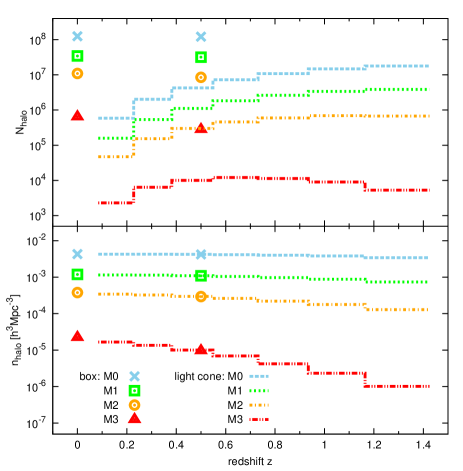
We are analysing two types of simulation outputs. For a detailed study of the dark matter growth we use the full comoving output at redshift and . For studying the bias estimators with minimal shot noise and sampling variance we use haloes identified in the comoving outputs at redshift and . The investigation of the redshift evolution of the bias and growth estimators is based on seven redshift bins of the light cone output with equal width of Mpc in comoving space over one octant of the sky. Fig. 1 shows the number and number density of haloes in the four mass samples for the comoving output and the light cone with respect to the redshift.
3 Growth and Bias Estimators
3.1 The growth factor
The large scale structure in the distribution of galaxies, observed today in cosmological surveys, is believed to originate from some small initially gaussian matter density fluctuations that grew with time due to gravitational instabilities. Since the way the Universe is expanding has an impact of the growth of structures, one can use measurements of the growth to put constraints on various cosmological models.
We adopt the common definition for density fluctuations, given by , where is the density at position smoothed (with a spherical top-hat window) over the radius , while is the mean density of the Universe. In the linear regime (large smoothing scales) density fluctuations of matter evolve with the redshift in a self similar way, thus
| (2) |
The reference redshift is usually arbitrarily chosen to be today, i.e. . In the CDM model the growth factor depends on cosmological parameters via the Hubble expansion rate
| (3) |
where and are the densities of matter and dark energy respectively, and the growth factor is then given by:
| (4) |
However, in general is also sensitive to modifications of the gravity action on cosmological scales (e.g. see Gaztañaga & Lobo 2001 and references therein). Measurements of the growth factor as a function of redshift can therefore be used to constrain cosmological models and understand the nature of cosmic expansion.
In practice, instead of computing the integral equation (4), one can also approximate the growth factor with an analytic expression, which is accurate at any redshift for a flat CDM model. This approximations can be obtained in two steps. First, on deriving equation (4) one can express the growth factor in terms of the growth rate
| (5) |
where . It follows that
| (6) |
which is an exact solution for any CDM (i.e. can be characterised by a curved space) cosmological model. Second, for a spatially flat universe, we can use the growth index defined as
| (7) |
Wang and Steinhardt (1998) found that it can be approximated by
which provides a relative precision of % on the growth factor. Recently Steigerwald et al. (2014) found an even more precise expression
which increases the accuracy of equation (6) to better then % at all redshift ().
Measuring the growth factor using equation (2) requires knowledge of the matter density fluctuations at different redshifts, while in practice only galaxies can be observed as biased tracers of the matter field. In the following sections we describe how we quantify and measure this galaxy bias.
3.2 The local bias model
Our bias estimations are based on the local bias model (Fry & Gaztanaga 1993), which assumes that the galaxy (number density) fluctuation is a function of the matter density fluctuation at the same location: , while both fluctuations are smoothed at the same scale . For sufficiently large smoothing scales the density fluctuations become small and we can expand this function, i.e. as in equation (1). For third-order statistics it is enough to stop the expansion at quadratic order (e.g. see Fry & Gaztanaga 1993)
| (8) |
where and are, respectively, the linear and quadratic bias parameters which we are measuring. The term ensures that , where denotes the average over all spatial positions. Besides small density fluctuations, such a model for the bias assumes that neither the environment nor the velocity field has an impact on galaxy formation.
Recent studies have shown, that the local assumption might not be accurate for small smoothing scales when is large (Baldauf et al., 2012; Chan et al., 2012).
Using the information contained in the large scale distribution of galaxies at different scales we measure bias and growth with second- and third-order statistics, as described in the following sections.
3.3 Growth factor from two-point correlation
The spatial two-point correlation of density fluctuations can be defined as the mean product of density fluctuations at the positions that are separated by the distance ,
| (9) |
Note that the two-point correlation function depends only on the separation and thus is not sensitive to the shape of over-densities. This is in contrast with higher-order correlations: with three points we will also be able to measure deviations away from the spherically symmetric profile (Smith et al., 2006).
From equations (2) and (9) one can derive that the growth factor is related to the two-point correlation of matter as
| (10) |
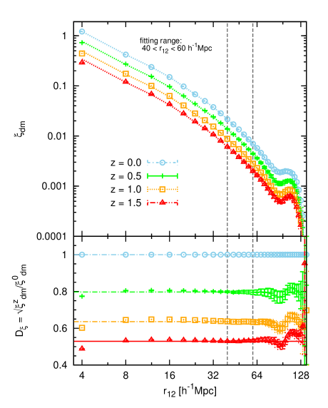
Our measurements of the matter correlation function in the MICE-GC simulation, presented in Fig. 2, indeed show a linear relation between the matter two-point correlations at different redshifts with respect to on a wide range of scales. Note how at scales around Mpc the BAO peak induces some oscillations around the linear model, but the model works well for intermediate scales of Mpc.
We measured the two-point correlation by dividing the simulation volume into cubical grid cells and assigning density fluctuations to each of these cells. We then calculate the mean product of density fluctuations in grid cells that are separated by according to definition (9). The measurements shown in Fig. 2 are based on Mpc grid cells. Errors are derived by Jackknife resampling as described in Section 3.6.
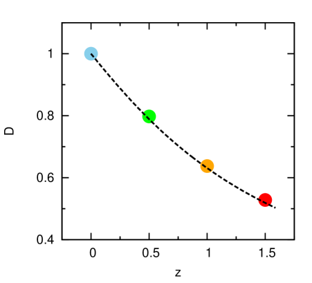
As shown in Fig. 3, there is a good agreement between the growth factor measurements from the two-point correlation (symbols) and the theoretical prediction from equation (4) (dashed line) for the cosmology of the MICE-GC simulation.
Deviations between predictions and measurements are at the sub-percent level and result from to non-linearities 777The increase of the deviations with redshift results from non-linearities in at . Since we use the latter as normalisation, deviations between predictions and measurements transfer to the higher redshifts. If we use at high as normalisation, as we do it later in the light cone, this effect goes into the opposite direction.. This result demonstrates that, in principle, we can obtain constrains on cosmological models by just measuring the two-point correlation function of matter.
However such constraints are difficult to realise as we have to infer the correlation of the unobservable full matter field from the correlation of the observed galaxy distribution. A simple relation between the two-point correlation functions of matter and galaxies can be obtained by inserting the model for galaxy bias, given by equation (8), into the definition of the two-point correlation (equation 9). At leading order
| (11) |
This relation only holds for sufficiently large separations , where we can neglect terms of order , and small density fluctuations in equation (8). To estimate the linear bias from we define
| (12) |
which is expected to be independent of separation in the large scale limit. In the following sections we will estimate from two other estimators ( and ) based on third-order statistics and we will probe how they compare to each other.
The correlation functions of the halo samples M0 - M3, calculated with Mpc grid cells, are shown in the top panel of Fig. 4 together with the corresponding measurements for the dark matter field. The ratios of the matter and halo correlations, shown in the bottom panel, confirm that both quantities can be related by the scale independent bias factor between Mpc. We expect that at the mass and scale range of our analysis (Crocce et al., 2013). To estimate we perform a -fit to the ratio of the halo and matter two-point correlation in the aforementioned scale range (see Subsection 3.6 for details). We find the values to vary between and . Values are smaller at compared to . Restricting the fitting range to larger scales (Mpc) also reduces the . Both findings are expected since non-linearities enter equation (12) at small scales and low redshift. However, restricting the fit to larger scales, as mentioned before, causes a maximum change in bias values is percent. We therefore consider our measurements as relatively robust, compared to the bias measurements from higher order statistics.
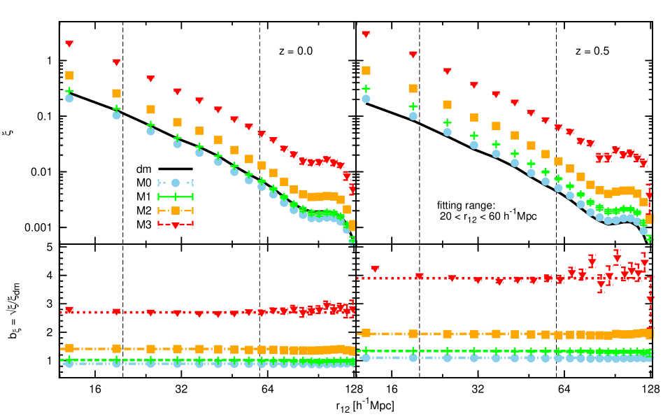
The fitted bias factors (bottom panel of Fig. 4) reveal the well known increase of bias with the mass and redshift of the halo samples.
The results described above allow us to estimate the growth factor of matter fluctuations from equation (10) in terms of galaxy (or halo) correlation functions as:
| (13) |
where the growth factor is normalised to unity at an arbitrary redshift (i.e. ). The bias ratio is defined as
| (14) |
and the galaxy (or halo) growth factor is:
| (15) |
Both definitions (14) and (15) refer to large scales, i.e between - Mpc, while we find changes in the results at the percent level when we vary the fitting range. The bias at the two different redshifts and does not need to refer to the same galaxy (or halo) populations. In Section 4.2 we demonstrate that taking different halo masses across the explored redshift range does not lead to unexpected growth measurements.
Equation (13) shows that the matter growth factor, measured from the galaxy (or halo) two-point correlation functions at different redshifts is fully degenerate with the ratio of the linear bias parameters. We therefore need an independent measurement of the bias ratio to break this degeneracy.
Note that the absolute values of the bias parameters, and , do not need to be measured separately for measuring the differential growth factor between two redshift bins, as it is commonly done. Instead of the absolute bias values, we only need to measure their ratio , which can be obtained directly from third-order galaxy correlations without assumptions on the clustering of dark matter, as we will explain in Subsection 3.4.
By measuring the differential growth factor between two nearby redshift bins and one can also estimate the (velocity) growth rate defined in equation (5) at the mean redshift . Since the growth rate is defined as logarithmic derivative of the growth factor, it follows that
| (16) |
Our new approach of measuring the bias ratio with third-order galaxy correlations will enable us to measure the growth factor and the growth rate of the full matter distribution directly from the distribution of galaxies (or haloes) without assumptions on the clustering of dark matter, providing a new model independent constrain on cosmological parameters. The same approach represents an additional tool to measure , which is independent of redshift space distortions method (Kaiser, 1987). Note that we do not need to select the same type of objects (with respect to the halo mass) at the different redshifts. This feature allows for maximisation of the galaxy number density at each redshift.
3.4 Bias from the three-point correlation
In analogy to the two-point correlation, we can define the three-point correlation as
| (17) |
where the vectors form triangles of different shapes and sizes. In contrast to the two-point correlation function is sensitive to the shape of the matter density fluctuations. To access this additional information, we fix the length of the two triangle legs and while varying the angle between them, . In the following we will therefore change the variables for characterising triangles from to . Throughout the analysis we use triangles with configurations, which restricts the minimum scale entering the measurements to the size of the smaller triangle leg . Choosing configuration, such as would introduce non-linear scales when triangles are collapsed ().
For detecting the triples we employ the algorithm described by Barriga and Gaztañaga (2002), using the same kind of mesh as for calculating the two-point correlation with and Mpc grid cells. From the three-point correlation we then construct the reduced three-point correlation, introduced by Groth and Peebles (1977) as
| (18) |
where .
Perturbation theory shows that, to leading order in the dark matter field, (hereafter referred to as Qdm) is independent of the growth factor. This is because , so drops in the ratio above (Bernardeau, 1994; Kamionkowski and Buchalter, 1999), but for galaxies depends on the bias parameters. These properties enable us to measure and and break the growth-bias degeneracy in equation (13) (Frieman and Gaztanaga, 1994; Fry, 1994; Bernardeau et al., 2002).
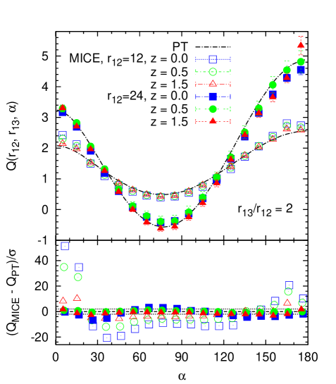
We test the assumption that is independent of the growth factor by comparing measurements at different redshifts and scales in the MICE-GC simulation with theoretical predictions derived from second-order perturbative expansion of and (Bernardeau et al., 2002; Barriga and Gaztañaga, 2002). The predictions are based on the MICE-GC CAMB linear power spectrum. Fig. 5 shows at , and for triangles with Mpc and Mpc. The measurements are based on a density mesh with Mpc grid cells, which is the highest available resolution (see Table 2 for details). As for the two-point correlation we derive errors for by Jackknife resampling (see Section 3.6). The values of show the characteristic u-shape predicted by perturbation theory, which results from the anisotropy of the shape of matter fluctuations. The amplitude of increases with triangle size because of the steeper slope in the two-point linear correlations at larger scales. Also depends only weakly on redshift while deviations between predictions and measurements become more significant at low redshift and small scales (see bottom panel of Fig. 5). The same effect has been reported by Fosalba et al. (2013a), who also find that the deviations decrease, when predictions are drawn from the measured instead of the CAMB power spectrum. Furthermore, these authors demonstrated that additional contributions to these deviations can result from the limited mass resolution of the simulation, especially at small scales and high redshift.
3.4.1 Non-linear bias
A simple relation between the bias in the local model and can be derived in the limit of small density fluctuations and large triangles by using equation (8) with the definitions (9), (17) and (18), and keeping second-order terms in the perturbative expansion (Frieman and Gaztanaga, 1994):
| (19) |
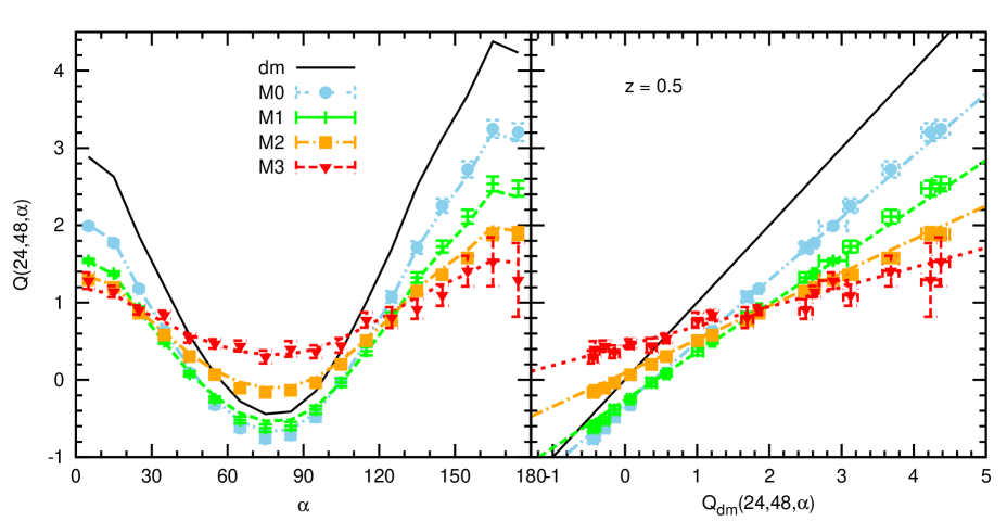
Instead of using , we could also use the corresponding predictions, shown in Fig. 6. However, this would introduce uncertainties in the bias measurement, due to the mismatch between measurements and predictions. We interpret the parameters and as the first- and second-order bias parameters and respectively, while we expect this interpretation to be valid only in the linear regime at scales larger than roughly Mpc. We use the notation instead of to refer to the fact that we are estimating with .
To measure the bias we computed for the four mass samples M0 - M3 at redshift and using triangles of various scales with configurations. The triangle legs consist now of and grid cells (see Table 2 for details). We vary the size of the triangles by changing the size of the grid cells. This reduces computation time, since the number of grid cells in the simulation volume required for the measurement is minimised. Our bias measurements from can vary by less than , when we increase the number of cells per leg instead of increasing the cell size to measure at larger scales. We show and discuss this effect in Appendix A.
Our results for Mpc triangles, shown in the left panel of Fig. 6 reveal a flattening of for high mass samples, as expected from equation (19) since increases with halo mass. In the right panel of the same figure we demonstrate that the linear relation between and , given by equation (19) is in reasonable agreement with the measurements. We perform -fits of the dark matter results to those of the four halo samples via equation (19) as described in Subsection 3.6 and obtain the bias parameters and . These fits, shown as colored lines in Fig. 6, have the strongest deviations from the measurements at the smallest and highest values of , which might result from measurements at small angles dominating as those have the smallest errors. The corresponding minimum values of per degree of freedom (given in the caption of Fig. 6) decrease for higher mass samples as the errors of increase. In general we find a decrease with mass, scale and redshift. Note that these results are affected by the covariance matrix in the fit which we only know roughly from the Jackknife sampling (see Section 3.6 and Appendix A).
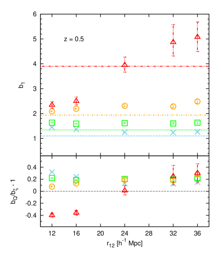
In order to use the bias parameter to measure the growth factor via equation (13) we first need to quantify deviations between and , i.e. the linear bias inferred from the two-point function and the one from in the fit to equation (19). If the local bias model approximation works well, then we would expect . A comparison is shown for different triangle scales and mass ranges in Fig. 7. In the top panel we show the linear bias derived with and at redshift as lines and symbols respectively.
In bottom panel of Fig. 7 we see that is up to higher than at large scales, while differences increase for smaller scales and larger values of . Such deviations between and have also been reported by, e.g. Manera and Gaztañaga (2011), Pollack et al. (2012), Baldauf et al. (2012), Chan et al. (2012), Moresco et al. (2014). Furthermore we find that for M3 is under predicted at small scales in contrast to results for the lower mass samples. Deviations for small triangle sizes indicate departures from the leading order perturbative expansion in which equation (19) is valid, while the strong deviations for the sample M3 suggest that the quadratic expansion of the bias function might not be sufficient for highly biased samples. Furthermore, differences between and are expected due to non-local contributions to the bias function, as it has been shown in -space by Chan et al. (2012). Performing the same analysis at redshift gives very similar results, which are shown in Fig. 20 of the appendix. We find in that case slightly larger deviations at small scales presumably due to a higher impact of non-linearities on the measurement. The overestimations at large scales are slightly smaller possibly as a result of smaller bias values at low redshift. We will show in a second paper that deviations between and decrease, when galaxy-matter-matter cross-correlations instead of galaxy-galaxy-galaxy auto-correlations are analysed. In the following we will focus on the results for Mpc which is a compromise between having small errors and sufficiently large scales for linear bias estimation.
3.4.2 Bias ratio from at different redshifts
A fundamental limitation for the growth factor measurement described in Section 3.3 is its dependence on the dark matter correlations, which cannot be directly observed. This problem is usually tackled by employing predictions for the dark matter correlations from N-body simulations or perturbation theory (see e.g. Verde et al., 2002; McBride et al., 2011; Marín et al., 2013). Alternatively weak lensing signals can be used as a direct probe of the total matter field (Jullo et al., 2012; Simon et al., 2013). Both approaches can add uncertainties and systematic effects to the galaxy bias measurement and will therefore affect constrains of cosmological parameters derived from the growth factor.
We therefore introduce a new approach for measuring the growth factor based on the following consideration: in equation (13) we see that for measuring the growth factor we only require knowledge about the ratio of the linear bias parameters at the redshifts and , while the absolute bias values are irrelevant. With the three-point correlation function we can measure this ratio directly from the distribution of galaxies without knowing . We can write equation (19) for the two redshifts and and combine them via under the assumption that is independent of redshift, as shown in Fig. 5. We find
3.5 Bias from third-order moments and
Here we are interested in the joint one- and two-point third-order cumulant moments taken at the locations and . We will estimate the first and second-order biasing coefficients by combining the skewness and reduced correlator . The skewness is the ratio of the one-point third-order cumulant, , and the one-point variance, , squared:
| (21) |
e.g. see equation (24) in Goroff et al. (1986). The reduced correlator (Bernardeau, 1996) is defined as the ratio between the joint two-point 3rd order cumulant, over the product of the variance and the two-point correlation function :
| (22) |
Note that, due to the same isotropic property as for the two-point correlation function, depends on the separation and not on the shape of the over density. The same happens for , which is a spherical average over some fix smoothing radius . Both, the skewness and the correlator , can be seen as two different collapsed forms of the reduced smoothed three-point correlation function , i.e. and .
3.5.1 Non-linear bias
Since it has been shown (Fry and Gaztanaga, 1993; Bel and Marinoni, 2012) that the local non-linear bias model conserves the hierarchical properties of both, cumulants and correlators of matter, one can express such quantities for any biased tracers (haloes or galaxies) with respect to the linear and quadratic bias coefficients
| (23) |
| (24) |
Following an orginal idea of Szapudi (1998), Bel and Marinoni (2012) worked out the explicit expressions of the bias coefficients up to fourth order. Since in the present paper we focus on the quadratic biasing model we recall the expressions they obtained at second order. By combining equations (24) and (23) one can find
| (25) |
| (26) |
As in the case of we interpret the parameters and as estimators of the first and second-order bias coefficients and respectively, while we expect this interpretation to be valid only in the perturbation theory regime.
In practice, the skewness and the reduced correlator can be estimated once the density fluctuations of haloes and matter ( and respectively) have been smoothed on a scale . In order to simplify the interfacing with theoretical predictions it is common to use a spherical Top-Hat window to smooth fluctuations. This is done by the count-in-cell estimators for the discrete and , which are described in Bel and Marinoni (2012) and used in this analysis. We correct these estimations from shot noise by assuming the local Poisson process approximation (Layser, 1956). Note that, in order to be able to handle the large number of dark matter particles, we use only of the total number of particles in the dark matter simulation output. This introduces additional shot noise errors but we have tested that it does not affect the measurements. To measure , we set up a regular grid of spherical cells. From the number of dark matter particles per cell we derive the corresponding number count fluctuations (), which we use to estimate the skewness via
where is the number of particles per grid cell, averaged over the volume of the simulation box.
The reduced correlator, , is measured via the two-point count-in-cell estimator (Bel and Marinoni, 2012). We therefore set up a regular grid of spherical cells, which are separated by two times the smoothing radius (hereafter referred to as seeds) and place an isotropic motif of spheres around each seed at separation . The two-point moments of the density field are then measured as the correlation between density fluctuations in the spheres of the motif and those in the seeds. This method allows for measurements of two-point statistics, even in the low separation limit when the spheres of the motif touch the spheres of the seeds, without being affected by any choice of distance bins. As for the skewness, we correct for shot noise assuming a Poisson sampling, which leads to
Once we have measured the skewness and the reduced correlator, the linear and quadratic bias and can be estimated for any chosen smoothing radius and for any ratio with equation (26). Errors of the measurements are computed by Jackknife resampling, as described in Section 3.6.
A theoretical prediction for the skewness and the reduced correlator can be derived with perturbation theory (PT, Bernardeau, 1992, 1996):
| (27) |
| (28) |
where and are, respectively, the logarithmic derivatives of the variance and the two-point correlation function of the smoothed field of density fluctuations with respect to the smoothing radius . Note that expression (28) has been obtained in the large separation limit ().
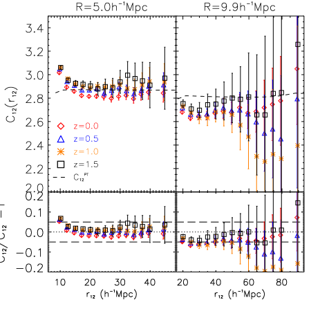
Fig. 8 gives an insight into the accuracy of the theoretical prediction of the reduced correlator from equation (28) for two different smoothing radii . The results, shown in Fig. 8 also show that on a wide range of separations (- Mpc) estimating the correlator at different epochs has no significant impact on the measured value, as predicted by perturbation theory. In fact, the values estimated at the four considered simulation snapshots (, , and ) vary by less than % (bottom panel).
The agreement with perturbation theory requires two important ingredients. First that the separation is much larger than the smoothing scale. Second, that we include the term in the prediction (Bel and Marinoni, 2012). Previously, this term was considered negligible (Bernardeau, 1996; Gaztañaga et al., 2002) and this resulted in a mismatch with numerical simulations, attributed to non-linear effects in the spherical collapse model (Gaztañaga et al., 2002).
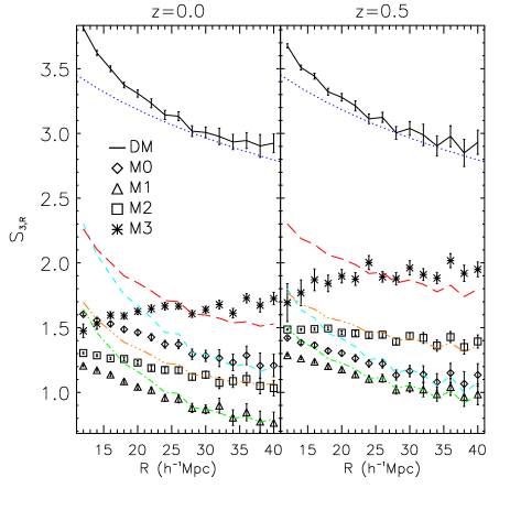
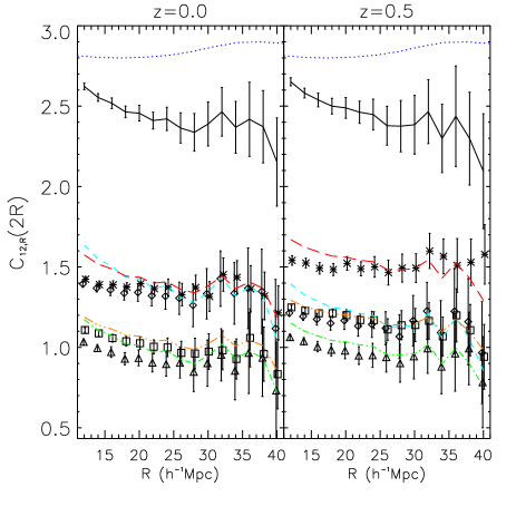
To increase the statistical signal of our measurements, we set the correlation length to be twice the smoothing radius, i.e. . The cells, used for the measurements, are consequently positioned side by side.
The Jackknife errors of from the dark matter field increase with redshift. This can be explained by shot noise being redshift independent as the number of particles is conserved, while the amplitude of the correlation decreases with redshift, causing smaller signal-to-noise ratios. Furthermore, one could expect that shot noise has a higher impact on at small smoothing scales since the smoothing window encloses on average less particles. However, we observe the opposite trend, presumably because a larger smoothing scale implies a smaller number of independent measurements due to the finite comoving volume of the simulation. This also explains the increase of errors with separation .
and measurements of the MICE-GC dark matter field are presented in Fig. 9, where they are contrasted with the corresponding quantities measured for haloes. At large smoothing scales the measurements for dark matter are in good agreement with the prediction from equation (27), represented by the blue dotted line. At small smoothing radii ( Mpc) we find the measurements to be significantly higher than the predictions. For haloes we can see that does not increase monotonically with mass. In fact, at Mpc and , for the low mass sample M0 the skewness is around , then drops down to for M1, increases to for M2 and finally reaches the value for the high mass sample M3. A similar tendency is observed at higher redshift. This non-monotonic behavior is qualitatively expected by the spherical collapse (Mo et al., 1997) and ellipsoidal collapse (Sheth et al., 2001) predictions and is in quantitative agreement with the measurements of Angulo et al. (2008), performed in a different simulation with a lower mass resolution and on a smaller mass range than the one reachable with the MICE-GC simulation.
The bottom panel of Fig. 9 shows for the first time how the mass of the chosen haloes affects the reduced correlator, . Comparing the effect of biasing on the shape of with its effect on , one can see that both follow the local bias model for large smoothing radii . The local bias model seems to be less accurate for as a function of , since its shape is systematically affected in a non-linear way. Moreover, we find the shape modification to increase with halo mass. Despite the fact that the predictions from equation (28) reproduce the large scale behavior of for haloes, we confirm significant deviations from the dark matter measurements at small separation (), even after taking into account the -term. But note that equation (28) has been obtained in the large separation limit (), so this is not totally unexpected. However, one can see in Fig. 8 that for larger separations the theory is in remarkably good agreement with measurements even for small smoothing radii such as Mpc. The local bias model works for if we use the matter measurements as input, despite their disagreement with perturbation theory. This is because the local model is an expansion on but does not require .
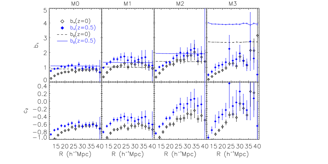
Turning to bias estimators, using equations (25) and (26) we measured and in each mass sample at both redshifts with respect to the smoothing radius . Measurements are displayed in Fig. 10, together with the bias estimator previously described. Estimators in equation (25) for and exhibit a significant scale dependency before converging to a constant value. This allows us to set up effective scale ranges in the fitting procedure used to measure the linear and quadratic bias. Comparing the scale dependency obtained for the various mass bins and redshifts we conclude that above Mpc both and are independent from the considered smoothing scale. We therefore measure them by performing a fit between and Mpc. As we showed that the shape of is highly affected at small scales, in particular at high halo masses, we can reasonably conclude that, on one hand, the scale dependency of and results from the skewness of haloes and, on the other hand, the large discrepancy observed between and (right panel of Fig. 10) is due to an underestimation of the skewness for massive haloes (we discuss this effect in Section 4.1).
3.5.2 Bias ratio from at different redshifts
In Subsection 3.4.2 we introduced a way of estimating the bias ratio using to measure the linear growth of structures directly from galaxies (or haloes), i.e. without assuming any modelling of the power spectrum nor of the bispectrum of matter fluctuations. Following the same idea we show now that we can measure using the estimator from equation (25) at the two redshifts: and . Assuming that does not depend on redshift, it is straightforward to show that:
| (29) |
The assumption that does not evolve with redshift is strongly supported by theory and simulations. Both and are expected to be weakly sensitive to redshift in perturbation theory. Measurements, shown in Fig. 8, illustrate that is weakly affected by redshift evolution, while results in Fig. (9) show that, on large scales ( Mpc), the skewness does not present significant redshift dependency (see also Bernardeau et al. (2002) and references therein).
3.6 Errors estimation and fitting
Since we use either one simulation at various comoving outputs (, , and ), or one light cone, we estimate the errors of , , , , , , , , and measurements by Jackknife resampling. The Jackknife samples of the complete comoving output are constructed from cubical sub-volumes while in case of the light cone we use angular regions (with equal volume at each redshift bin) in right ascension and declination on the sky. Following Norberg et al. (2009), we generate for any statistical quantity a set of pseudo-independent measurements (), from which we compute the standard deviation around the mean (computed on the complete volume) as
| (30) |
where is the number of Jackknife samples.
For all three bias estimations , or , we use the same fitting procedure, which takes into account the covariance between , and measurements at different separations, opening angles and smoothing scales (, , respectively). The covariance matrix is computed from the deviation matrix , which in turn is estimated by Jackknife resampling as well: a measurement in the Jackknife sub-volume and for the separation, angle or scale is written . Each element of the deviation matrix is calculated as . Again the mean is the measurement on the complete volume. The covariance matrix can then be computed straightforwardly
| (31) |
The bias ratio can be fitted from results at different smoothing scales in a very simple way, because the first- and second-order bias coefficients can be estimated separately in the formalism (see equation (29)). Deriving is more complicated as it requires a two-parameter fit, due to the mixing of the bias coefficients (see equation (20)). The main problem arises from the fact that at a given redshift the errors of are correlated between the various angles. Furthermore the reduced three-point correlation can also be correlated between the two redshifts and , where is the reference redshift. Based on equation (20), we define the variable
| (32) |
and vary and in order to obtain for all angles . In other words we want to measure the posterior probability distribution (hereafter referred to as likelihood ) of the two parameters and given that is expected to be . Assuming a multivariate normal distribution of , one can write the log-likelihood as for measuring a given
| (33) |
where is the covariance matrix of the , is a normalisation constant and . Note that, if the covariance matrix does not depend on the parameters of the model, then the second term in expression (33) can be absorbed in the normalisation constant . However, from definition (32) follows that explicitly depends on the fitting parameters and . It can therefore be obtained from the covariance matrix of , and from the cross-covariance of and :
| (34) |
which explicitly shows the dependency of the covariance matrix on the fitting parameter . Note that and are respectively the covariance matrix of and computed with equation (31). The cross-covariance matrix is defined as
| (35) |
where is the number of elements in both and . In practice we shall neglect the correlation between redshift bins, so that in equation (34). Otherwise the inverse covariance matrix had to be computed for each tested value of . The estimate of and its error are obtained by marginalising over the parameter via the posterior marginalised log-likelihood
Testing the assumption that measurements at different redshifts are uncorrelated, we verified that the correlation coefficient remains very small compared to unity. It follows that the square of the relative error for the bias ratio is obtained by summing in quadrature the relative errors of and . Then, since and are third-order estimators, we checked that the error of the halo growth factor is negligible with respect to the error obtained for the bias ratio .
4 Results
As we have pointed out in the sections 3.3-3.5 we use growth independent bias measurements from third-order statistics to break the growth-bias degeneracy that appears in growth measurements from two-point correlations. This approach is limited by the accuracy and the precision with which third-order statistics can measure galaxy bias. We study the differences between bias from second- and third-order correlations for different redshifts and halo mass ranges and present the results in Section 4.1. In Section 4.2 we show the resulting estimations for the linear growth measurements.
Alternatively to the direct approach of growth measurement described above, we have introduced a new method which does not require any modelling of third-order clustering of dark matter. It takes advantage of the fact that only the ratio of the bias parameters at two redshifts needs to be known to break the growth-bias degeneracy. This bias ratio can be directly measured from third-order statistics of the halo field (see Section 3.3-3.5). In Section 4.2.2 we compare growth factor measurements from our new method and the more common method of combining second- and third-order statistics with theoretical predictions (or simulations) for the dark matter field. In Section 4.2.3 we present growth rate measurements derived with and without third-order correlations of dark matter.
4.1 Bias comparison
4.1.1 Measurements in the comoving outputs
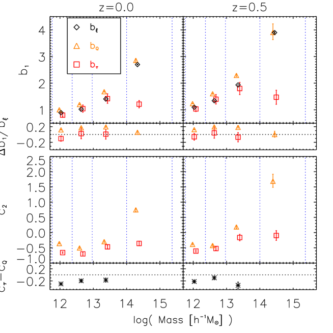
In Fig. 11 we show the values of the linear and quadratic bias parameters and , measured with the and estimators ( and ) in the comoving outputs at redshift and . The bias parameters from are estimated from triangles with fixed legs of and Mpc (see Table 2 for details) using opening angles with values between 0 and 180 degree as shown in Fig. 6. The bias estimations are based on fits of and between Mpc using () configurations (see Fig. 10). All error bars denote the standard deviation derived from Jackknife samples as described in Section 3.6.
In the same figure we compare our measurements of the linear bias parameter from third-order statistics with computed from the two-point correlation between and Mpc by showing the absolute values as well as the relative differences. In case of we show the absolute instead of the relative difference since we have no reference values from two-point correlations.
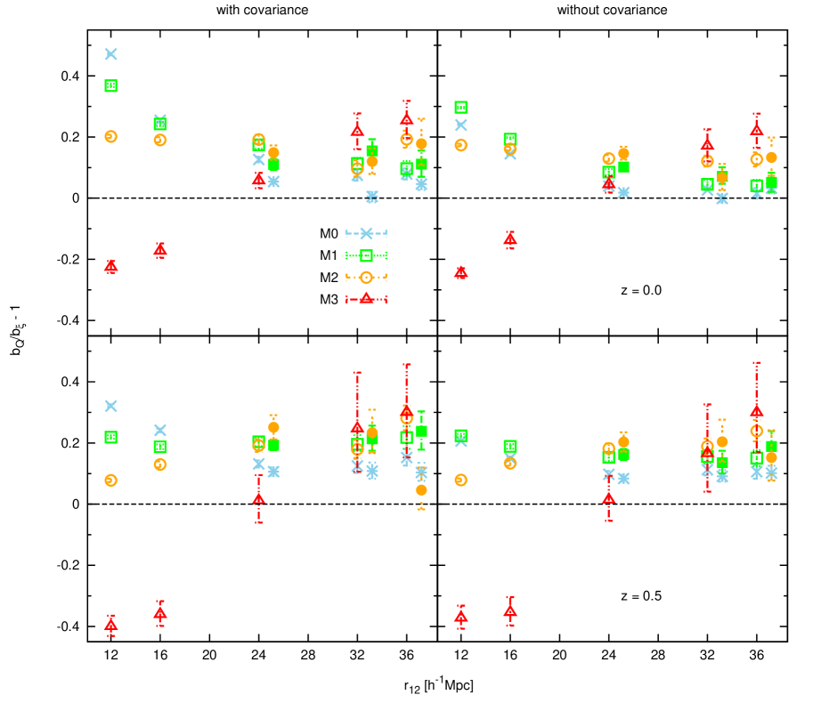
The linear and quadratic bias parameters from both estimators increase with mass and redshift, while their absolute values differ in several aspects. As demonstrated already in Fig. 7, overestimates the linear bias in all mass samples by a factor between with respect to . The good agreement between and for the high mass sample M3 only appears for the chosen triangle configuration of (24,48,). The overestimations confirm findings from Manera and Gaztañaga (2011), Pollack et al. (2012) and Chan et al. (2012), while the large volume and resolution of the MICE-GC simulation allows us to extend this bias comparison to a wider range of masses than probed previously. Chan et al. (2012) argued that the mismatch of the linear bias by is expected from non-local contributions to the bias function. But note that the comparison with the results here is not direct. Our results are in configuration space (not in Fourier space), for halo-halo-halo correlations (not halo-matter-matter) and for a different cosmology. Moreover, the deviations found in Chan et al. (2012) depend linearly on the value, while we find here a shift by a factor that is roughly independent of mass (and therefore of ). We will explore some of these differences in a separate paper.
On the other hand, the bias estimation, , shows a good agreement with for the lower mass bins, but at a price of larger errors. This suggests that the estimator is less affected by such non-local contributions than , which is also expected from theory, since the isotropy of the estimators of and could wash out the non-local effects. strongly underestimates the linear bias parameter for the highest masse bin (M3). This might be caused by discreteness effects which need to be corrected in the estimation (note that this does not affect ). Here we have used Poisson shot noise corrections, but these are likely to be incorrect for massive haloes because of exclusion effects (see e.g. Manera and Gaztañaga, 2011). As a result, for haloes which are too massive, the correct estimation of the skewness is far from being trivial. Assuming a wrong shot noise correction leads to an underestimation of , which causes to be over-predicted and translates for the estimator into a large underestimation of the linear bias and presumably of the second-order bias (left panel of Fig. 11).
Besides non-local terms, the discrepancies between , and , highlighted in Fig. 11, can be caused by various other effects, such as stochasticity or contributions of higher-order terms to the bias expansion (equation 8). The Jackknife estimation of the errors and the covariance matrix introduces an additional uncertainty in the bias measurement (see Appendix A).
The larger errors of the measurements with respect to those from are a consequence of the larger errors in and with respect to in Fig. 6 and 9. The larger errors in and result from the larger smoothing scales compared to those used to compute Q, which leads to a lower number of independent measurements. An additional contribution to the higher scatter of the and results from the grid used in the estimation. It neglects roughly of the volume since the seeds do not overlap with each other. An additional minor source of error comes from the fact that, for practical reasons, only of the total number of dark matter particles are used to measure and of matter, which is discussed in Subsection 3.5.1. For both and errors could be improved by including more configurations and optimal weighting.
Regarding the quadratic bias coefficient we found that the estimated values of and are in significant disagreement for mostly all mass bins. We will study this results in more detail by comparing similar estimations from halo-matter-matter cross-correlation with predictions from the peak background split model in a separate paper.
4.1.2 Measurements in the light cone
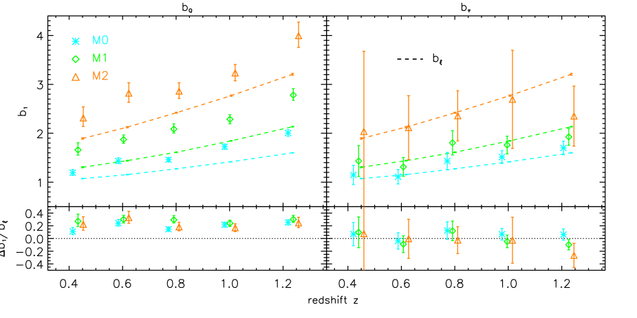
To be more realistic, we conduct bias measurements in a light cone, which is constructed from the MICE-GC simulation and includes redshift evolution of structures. The total volume probed by the light cone is about Gpc3 and we consider an octant of the sky (about 5000 deg2). We study the deviation between the different bias estimations in five redshift bins between using the mass samples M0, M1 and M2. We do not present results for the highest mass sample M3 and for smaller redshifts, since the results are strongly scattered due to small numbers of haloes (see Fig. 1). However, this mass and redshift range was previously analysed using the comoving outputs of the same simulation.
For measuring the bias we use the same (24,48,) configurations for as in the comoving output. In the case of we use () configurations as in the previous analysis and we perform a fit over the scale range - Mpc for the mass bins M0 and M1, while we restrict this range to - Mpc in case of M2. These new fitting ranges are motivated by Fig. 10, which shows that at the redshift the scale dependency of can be neglected on those ranges and for the corresponding mass bins. To maximize the statistical power of the estimator we now use overlapping cells to avoid neglecting roughly half of the data in the space between the seeds used to smooth the particle distribution. Note that in this case we estimate errors by Jackknife resampling of angular regions of the light cone (see Section 3.6).
The results for the and estimator are shown together with in Fig. 12. They confirm that tends to overestimate the bias for the lower mass bins by about . Moreover it shows that the ratio between and is roughly a constant with respect to the redshift or mass bins. On the other hand seems to be an unbiased estimate of the linear bias coefficient, while the measurements are noisier.
Since in our approach we aim at measuring the linear bias in order to extract information about the growth factor of linear matter fluctuations, we focus on deriving a direct measurement of it in the following section.
4.2 Growth Measurements
In this subsection we present the growth factor and the growth rate , measured in the MICE-GC light cone via the equations (13) and (16) respectively. We obtained these measurements with the linear bias , estimated with and (equation (20) and (25) respectively) at the redshift and the reference redshift . These growth measurements are compared to those from our new approach for measuring and via the bias ratio . We can derive directly by comparing and of galaxies (or haloes) at and (equations (20) and (29)). This new approach allows us to measure the growth of dark matter using only the observable second- and third-order galaxy (or halo) correlations without the corresponding dark matter statistics (see Sections 3.4 and 3.5).
4.2.1 Growth factor measured with and
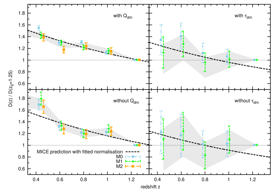
Fig. 13 shows measurements of the growth factor , derived from the mass samples M0, M1 and M2 in the MICE-GC light cone. Symbols denote results, which were derived by using the same mass bins at both redshifts, and . Exploring the variation of our results for different choices of mass bins, we measure the growth factor from all combinations of mass bins. The median growth factor and the median error from all combinations are shown as grey shaded areas in the same figure. The top panels show results, derived by using the bias parameters and (left and right respectively), which were measured at each redshift separately from equation (19) and (25). This approach requires the knowledge or modelling of the dark matter and . Note that we normalised all measurements with respect to the highest redshift bin by setting in equation (13). This allows us to have a normalisation, which is performed as much as possible in the linear regime and with the lowest possible sampling variance. The measurements are compared to the theoretical prediction from equation (4), shown as dashed lines in the same figure. We also show that combining different halo populations (halo mass) at different redshifts we obtain results which are consistent with those derived by following the same halo population across the considered redshift range. To be independent of the normalisation we -fit the normalisation of the predictions to the median measurements from all mass sample combinations (i.e halo populations).
Our results in Fig. 13 show that the growth factor, measured with the bias from the third-order statistics, decreases with redshift, as expected from predictions for the linear growth factor. In the case of (top left panel of Fig. 13) the good agreement between measured and predicted growth factor is remarkable since the bias estimation, on which the measurement is based on, shows a over estimation (see left panel of Fig. 12). We explain this finding by a cancellation in the bias ratio of the multiplicative factor by which is shifted away from . This cancellation also happens for the median results from all mass bin combination, since this multiplicative factor is similar for all masses and redshifts. Fluctuations of the growth factor measurements at high redshifts probably result from fluctuations in the bias measurements. We expect an additional uncertainty in the growth measurement from the resolution of the density grid, used for computing (see Appendix A). From equation (13) we estimate that the resolution error in propagates into as an error of below .
The growth factor measurements based on the estimator (top right panel) are significantly noisier than the estimation, as expected from the linear bias estimations displayed in Fig. 12. Note that the growth factor, measured via , appears to be more strongly biased at higher mass ranges. However, this is only the propagation of the statistical fluctuation of the bias measurements into the higher redshift bin, which is used to normalise the measured growth factor in all the other redshift bins (see Fig. 12). Thus, we can conclude the estimator provides an unbiased estimate of the growth factor.
4.2.2 Growth factor measured without and
In the bottom panels of Fig. 13 we show the growth factor measurements based on the new approach, which uses the bias ratios and derived from equations (20) and (29) (left and right respectively). This means that we compare the statistical properties only of the halo density field at different redshifts, without requiring knowledge about the dark matter quantities , . As in the top panels, the symbols denote measurements using the same mass bins at both redshifts, while median growth measurements and errors from all mass bin combinations are shown as grey shaded areas.
We find for both estimators slightly larger deviations from the linear theory compared to the results from the separate bias measurement, shown in the upper panels. This discrepancy tends to be larger as the redshift is decreasing, possibly due to three effects: i) noise in the measurements of third-order galaxy (or halo) correlations (, ) enters twice, ii) non-linearities in the dark matter field become stronger at small redshift, iii) sampling variance does not cancel out since the two halo correlations, on which the measurement is based on, come from different redshifts.
In practice that last point iii) will also affect the first method, which uses and to get the absolute bias at each redshift. In our analysis, sampling variance cancels out between redshifts because we use and measured in the same simulation where we measure the corresponding halo values and . In the analysis of a real survey this cancelation will not occur since one needs to use models for and .
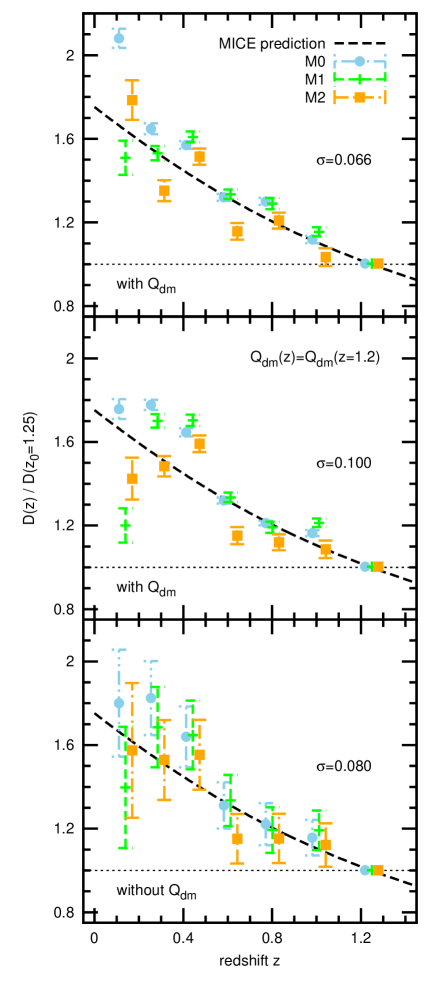
We demonstrate this effect in Fig. 14. To study how the fitting range affects the growth estimate we now restricted to opening angles between degree, excluding large triangles as we discuss later. The top panel shows the growth, measured with the separate bias estimates of , as shown on the top panel of Fig. 13. In the central panel we show the more realistic growth measurements based on the same approach, but instead of using the dark matter measurements in the same redshift as the halo measurements, we always use the dark matter results of from the highest redshifts bin (which is in good agreement with the results from the comoving output, as it contains more volume than the other redshift bins). Here, the sampling variance does not cancel, since the dark matter and halo correlations are measured at different redshifts. This results in a larger scatter in the central panel than in the top panel. Quantifying this scatter with respect to the predictions as confirms the visual impression (values are shown in Fig. 14). The latter approach in the central panel corresponds more closely to how the first method would be applied in a real survey: i.e. assuming a cosmology to run the dark matter model and running a simulation for that cosmology (sampling variance will not cancel as the simulation has different seeds than the real Universe). These latter growth measurements are distributed in a similar way around the theoretical predictions as the results derived from the ratio bias approach using and at the redshift and redshift , shown in the bottom panel of Fig. 14. This demonstrates that most of the difference between the top and bottom panels of Fig. 14 comes from the artificial sampling variance cancelation in the top panel.
The restriction of the opening angles to excludes widely opened triangles and is a possibility to decrease the impact of sampling variance on the measurements. However, comparing the growth in the bottom panel of Fig. 14 to the corresponding measurements for in the bottom left panel of Fig. 13 we find no significant improvement of the growth measurements from restriction of the opening angles possibly due to larger errors. The latter result from the smaller number of triangles.
4.2.3 Growth rate measured with and without
We derived the growth rate from the measured growth factor via equation (16). The product can also be probed by redshift space distortions, while our measurements represent an additional, independent approach to the growth rate. Especially at higher redshifts, where growth rate measurements via redshift space distortions are difficult to obtain, such additional information is valuable. Besides the relation to redshift space distortions another advantage of the growth rate with respect to the growth factor is that it is independent of the normalisation. The latter cancels out in the ratio of the growth factors, which appears in equation (16).
However, measuring via at a given redshift is not straightforward, since it depends on measurements at two different redshift. We derived at the redshift bin from growth factor measurements at and . This approach is motivated by the fact that the redshift bins have equal width in comoving space. Constrains of cosmological parameters with such measurements would require a more careful treatment of the assigned redshift. The employed growth factors are the median results, derived via from all mass combinations, which are shown as grey areas in the left panels of Fig. 13.
The results for from , measured with and without , are shown in Fig. 15. In both cases the measurements are strongly scattered around the theoretical predictions for the MICE simulation, while the scatter is stronger for results derived without . The increased scatter at lower redshifts probably results from the smaller volume of the light cone, which causes stronger fluctuations in (see Fig. 13). We also expect an uncertainty from the resolution of the density grid, used for computing (see Appendix A). From the equations (13) and (16) we estimate that the resolution error in propagates into as an error of below . Note that the errors that we find at high redshifts are comparable, or slightly better, than current errors from redshift space distortions (RSD) in the anisotropic 2-pt correlation function. Note that measurements from RSD directly constrain and not . Nevertheless, under some assumptions we can also infer from RSD and the typical errors found on SDSS, BOSS and WiggleZ are around 15-20% (Cabré and Gaztañaga, 2009; Blake et al., 2011; Tojeiro et al., 2012), which are comparable to the ones we find here.
The MICE prediction is computed from equation (7) with and . To compare the scatter in our measurements with variations of the growth rate for different cosmologies we also show predictions for and . We find that our errors in the measurements are larger than the expected variations in the growth rate due to cosmology. It would be worthwhile to conduct a similar comparison using larger mass bins and combining measurements from different scales and configurations of , to decrease the error, but the goal here is just to demonstrate the possibility of such measurements and the advantage of using it.
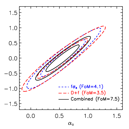
We also studied a test case where we compare the inference power of a measurement of with a measurement of and independently. To do so we simulated seven measurements of and of and at seven different redshifts (see caption of Fig. 16) and we compared the constraining power of the two methods in determining the growth index characterized by the two free parameters and . We stress that this analysis is purely illustrative, in the sense that we just compare the intrinsic potential of each method, i.e. we assume the same number of measurements at the same redshift and with the same relative errors. Fig. 16 shows that the constraining power is compatible for the two methods leading therefore to an improvement close to a factor of when combining them (black lines). However, note that in case of it is necessary to assume an external prior on the scalar amplitude of the initial power spectrum. We indeed should have taken a Gaussian prior on it (see second column of Table 2 in Planck Collaboration et al., 2013), however assuming that any dark-energy or modifications of gravity would kick in between redshift and , we equivalently assumed a Gaussian prior (with the same relative error) on the normalisation of the power spectrum at redshift . While for the method we propose, no priors on the scalar amplitude are assumed.
5 Summary & Discussion
The amplitude of the transverse (or projected) two-point correlation of matter density fluctuations allows us to measure the growth factor , which can be used as a verification tool for cosmological models. Galaxies (in our study represented by haloes) are biased tracers of the full matter field as their two-point correlation at large scales is shifted by a constant bias factor with respect to the matter two-point correlation. This bias factor is fully degenerate with . The reduced matter and galaxy third-order statistics are independent of , while the galaxy versions are sensitive to . Combining second- and third-order statistics could therefore enable us to break the growth-bias degeneracy, if the difference between the effective linear bias probed by both statistics is smaller than the errors required for the growth measurements.
In this paper we have tested these assumptions and verified how well we can recover the true growth of the new MICE-GC CDM simulation (Fosalba et al., 2013a; Crocce et al., 2013; Fosalba et al., 2013b) with them. We also further validate the MICE-GC simulation by comparing the linear growth with the two-point matter correlation (Fig.2 and 3) and the different third-order statistics of the matter field to non-linear perturbation theory predictions (Fig.5 and 8). In particular, previous analysis (Gaztañaga et al., 2002) found a mismatch between simulations and predictions for (Bernardeau, 1996), which we find here to originate from neglecting one of the smoothing terms (i.e. in Eq.28). After taking this into account, the MICE-GC simulations agrees well with predictions for all redshifts (see Fig.8). This, therefore, provides a validation of the approach adopted by Bel and Marinoni (2012) to measure the linear galaxy bias using only galaxy clustering.
The main goal of this paper is to compare bias (and the resulting growth) measurements from two different third-order statisticics proposed in the literature. One uses the reduced three-point correlation while the other uses a combination of the skewness and two-point third-order correlator, , which is called . We estimated these quantities from density fields of matter in the MICE-GC simulation and those of haloes in different mass samples, expanding previous studies significantly to a wider range of masses (between and M⊙) and redshifts (between and ) with values of the linear bias between and .
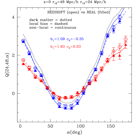
Our results in Fig. 11 show that the linear bias from , , systematically over estimates the linear bias from the two-point correlation, , by roughly at all mass and redshift ranges, whereas the linear bias from , , seems to be an unbiased estimator at the price of decreased precision. Non-local contributions to galaxy bias, like tidal effects, are anisotropic and therefore could be more important for than for , as is isotropic (i.e. it comes from higher-order one- and two-point correlations, while comes from three points). In Fig. 17 we illustrate the different impacts of the local bias model and the non-local model of Chan et al. (2012) with on (dashed and solid lines respectively). The non-local model seems to approximate measurements from halo samples better but there are still some discrepancies that we will explore in a separate analysis. Besides non-local contributions to the bias model, further reasons for the difference between and might be that non-linear terms in the bias function and the matter field have different impacts on and . In addition we found that estimations of the quadratic bias parameter from and can also differ significantly from each other.
Understanding the differences between , and is crucial for constraining cosmological models with observed third-order halo statistics. We will therefore deepen our analysis in a second paper by studying bias from halo-matter-matter statistics, direct analysis of the halo versus matter fluctuations and predictions from the peak-background split model to disentangle between non-linear and non-local effects on the different estimators.
For measuring the growth factor we have introduced a new method. This new method uses the bias ratio , derived directly from halo density fluctuations with reduced third-order statistics. Its main advantage with respect to the approach of measuring and separately is that it does not require the modelling of (third-order) dark matter statistics. Instead, it works with the hypothesis that
-
1.
the reduced dark matter three-point statistics is independent of redshift
-
2.
the bias ratio from two- and three-point statistics is equal.
The first assumption was tested in this study numerically, while the validity of the second follows directly from our bias comparison.
In general the comparison between from perturbation theory with measurements from our new method and the standard approach reveals a good agreement. In the case of we explain this result by a cancellation of the multiplicative factor by which is shifted away from in the bias ratio . The growth factor measured with has larger errors than the results from as a consequence of the larger errors in the bias estimation.
Our analysis shows that the new way to measure the growth factor from bias ratios is competitive with the method based on two separate bias measurements. While having larger errors the new method has the advantage of requiring much weaker assumptions on dark matter correlations than the standard method and therefore provides an almost model independent way to probe the growth factor of dark matter fluctuations in the Universe.
We demonstrated that besides the growth factor, , the growth rate of matter, , can also be directly measured from the galaxy (or halo) density fields with bias ratios from third-order statistics. This provides an alternative method to derive the growth rate, which is usually obtained from velocity distortions probed by the anisotropy of the two-point correlation function (RSD). The typical errors found on SDSS, BOSS and WiggleZ using RSD are around 15-20% (Cabré and Gaztañaga, 2009; Blake et al., 2011; Tojeiro et al., 2012), which are comparable to the ones we find in Fig. 15 when considering the high redshift bins (20%).
Given that the two methods explored here use different information from higher-orders correlation ( uses the shape, while uses collapse configurations) one can reasonably guess that the two methods are not strongly correlated. So a possible strategy would be to use the method (more precise) to measure the (velocity) growth rate and, in parallel, to use the method to extract the growth factor. This would help to break degeneracies between cosmological parameters in different gravitational frameworks.
Our analysis is performed in real space to have clean conditions for comparing different bias and growth estimates. This is a good approximation for the reduced higher-order correlations on the large scales considered in this study, as measurements in redshifts space always seem to be within one sigma error of the corresponding real space result (see Fig. 17). Note how the small, but systematic, distortions in redshifts space seem to agree even better with the local bias model than in real space on the largest scales.
Applying the methods described above to obtain accurate bias and growth measurements from observations will require additional treatment of redshifts space distortions or projection effects. Two possible paths could be followed. In a three dimensional analysis redshifts space distortions need to be modeled (e.g. Gaztañaga and Scoccimarro, 2005). The projected three-point correlation can also be studied separated by in redshift bins (Frieman and Gaztañaga, 1999; Buchalter et al., 2000; Zheng, 2004). Both ways will result in larger errors, but we do not expect this to be a limitation because our error budget is totally dominated by the uncertainty in the bias. A more detailed study of this issue is beyond the scope of this paper and will be presented elsewhere. Mock observations, like the galaxy MICE catalogues (see Crocce et al., 2013; Carretero et al., 2014) should be used to test the validity of such growth measurements under more realistic conditions.
Acknowledgements
Funding for this project was partially provided by the Spanish Ministerio de Ciencia e Innovacion (MICINN), project AYA2009-13936, Consolider-Ingenio CSD2007- 00060, European Commission Marie Curie Initial Training Network CosmoComp (PITN-GA-2009-238356) and research project 2009- SGR-1398 from Generalitat de Catalunya. JB acknowledges useful discussions with Christian Marinoni and support of the European Research Council through the Darklight ERC Advanced Research Grant (#291521). KH is supported by beca FI from Generalitat de Catalunya. He also acknowledges the Centro de Ciencias de Benasque Pedro Pascual where parts of the analysis were done. The MICE simulations have been developed at the MareNostrum supercomputer (BSC-CNS) thanks to grants AECT-2006-2-0011 through AECT-2010-1-0007. Data products have been stored at the Port d’Informaci Cient fica (PIC).
References
- Angulo et al. (2008) Angulo R.E., Baugh C.M., Lacey C.G., 2008, MNRAS, 387, 921
- Baldauf et al. (2012) Baldauf T., Seljak U., Desjacques V., McDonald P., 2012, Phys.Rev.D, 86, 083540
- Barriga and Gaztañaga (2002) Barriga J., Gaztañaga E., 2002, MNRAS, 333, 443
- Bel and Marinoni (2012) Bel J., Marinoni C., 2012, MNRAS, 424, 971
- Bernardeau (1992) Bernardeau F., 1992, ApJ, 392, 1
- Bernardeau (1994) Bernardeau F., 1994, ApJ, 433, 1
- Bernardeau (1996) Bernardeau F., 1996, A&A, 312, 11
- Bernardeau et al. (2002) Bernardeau F., Colombi S., Gaztañaga E., Scoccimarro R., 2002, Phys. Rept., 367, 1
- Blake et al. (2011) Blake C., et al., 2011, MNRAS, 415, 2876
- Buchalter et al. (2000) Buchalter A., Kamionkowski M., Jaffe A.H., 2000, ApJ, 530, 36
- Cabré and Gaztañaga (2009) Cabré A., Gaztañaga E., 2009, MNRAS, 393, 1183
- Carretero et al. (2014) Carretero J., Castander F.J., Gaztanaga E., Crocce M., Fosalba P., 2014, ArXiv e-prints
- Chan et al. (2012) Chan K.C., Scoccimarro R., Sheth R.K., 2012, Phys.Rev.D, 85, 083509
- Contreras et al. (2013) Contreras C., et al., 2013, MNRAS, 430, 924
- Crocce et al. (2013) Crocce M., Castander F.J., Gaztanaga E., Fosalba P., Carretero J., 2013, ArXiv e-prints
- Davis et al. (1985) Davis M., Efstathiou G., Frenk C.S., White S.D.M., 1985, ApJ, 292, 371
- de la Torre et al. (2013) de la Torre S., et al., 2013, A&A, 557, A54
- Feldman et al. (2001) Feldman H.A., Frieman J.A., Fry J.N., Scoccimarro R., 2001, Physical Review Letters, 86, 1434
- Fosalba et al. (2013a) Fosalba P., Crocce M., Gaztanaga E., Castander F.J., 2013a, ArXiv e-prints
- Fosalba et al. (2013b) Fosalba P., Gaztanaga E., Castander F.J., Crocce M., 2013b, ArXiv e-prints
- Frieman and Gaztañaga (1999) Frieman J.A., Gaztañaga E., 1999, ApJL, 521, L83
- Frieman and Gaztanaga (1994) Frieman J.A., Gaztanaga E., 1994, ApJ, 425, 392
- Fry (1994) Fry J.N., 1994, Physical Review Letters, 73, 215
- Fry and Gaztanaga (1993) Fry J.N., Gaztanaga E., 1993, ApJ, 413, 447
- Gaztañaga and Lobo (2001) Gaztañaga E., Lobo J.A., 2001, ApJ, 548, 47
- Gaztañaga and Scoccimarro (2005) Gaztañaga E., Scoccimarro R., 2005, MNRAS, 361, 824
- Gaztañaga et al. (2002) Gaztañaga E., Fosalba P., Croft R.A.C., 2002, MNRAS, 331, 13
- Gaztañaga et al. (2005) Gaztañaga E., Norberg P., Baugh C.M., Croton D.J., 2005, MNRAS, 364, 620
- Gaztanaga (1992) Gaztanaga E., 1992, ApJL, 398, L17
- Gaztanaga (1994) Gaztanaga E., 1994, MNRAS, 268, 913
- Gaztanaga and Frieman (1994) Gaztanaga E., Frieman J.A., 1994, ApJL, 437, L13
- Goroff et al. (1986) Goroff M.H., Grinstein B., Rey S.J., Wise M.B., 1986, ApJ, 311, 6
- Groth and Peebles (1977) Groth E.J., Peebles P.J.E., 1977, ApJ, 217, 385
- Guzzo et al. (2008) Guzzo L., et al., 2008, Nature, 451, 541
- Jullo et al. (2012) Jullo E., et al., 2012, ApJ, 750, 37
- Kaiser (1987) Kaiser N., 1987, MNRAS, 227, 1
- Kamionkowski and Buchalter (1999) Kamionkowski M., Buchalter A., 1999, ApJ, 514, 7
- Kovač et al. (2011) Kovač K., et al., 2011, ApJ, 731, 102
- Layser (1956) Layser D., 1956, AJ, 61, 1243
- Lue et al. (2004) Lue A., Scoccimarro R., Starkman G., 2004, Phys.Rev.D, 69, 044005
- Manera and Gaztañaga (2011) Manera M., Gaztañaga E., 2011, MNRAS, 415, 383
- Marín (2011) Marín F., 2011, ApJ, 737, 97
- Marín et al. (2013) Marín F.A., et al., 2013, MNRAS, 432, 2654
- Marinoni et al. (2005) Marinoni C., et al., 2005, A&A, 442, 801
- Marinoni et al. (2008) Marinoni C., et al., 2008, A&A, 487, 7
- McBride et al. (2011) McBride C.K., Connolly A.J., Gardner J.P., Scranton R., Scoccimarro R., Berlind A.A., Marín F., Schneider D.P., 2011, ApJ, 739, 85
- Mo et al. (1997) Mo H.J., Jing Y.P., White S.D.M., 1997, MNRAS, 284, 189
- Moresco et al. (2014) Moresco M., Marulli F., Baldi M., Moscardini L., Cimatti A., 2014, MNRAS, 443, 2874
- Norberg et al. (2009) Norberg P., Baugh C.M., Gaztañaga E., Croton D.J., 2009, MNRAS, 396, 19
- Pan and Szapudi (2005) Pan J., Szapudi I., 2005, MNRAS, 362, 1363
- Perlmutter et al. (1999) Perlmutter S., et al., 1999, ApJ, 517, 565
- Planck Collaboration et al. (2013) Planck Collaboration, et al., 2013, ArXiv e-prints
- Pollack et al. (2012) Pollack J.E., Smith R.E., Porciani C., 2012, MNRAS, 420, 3469
- Reid et al. (2012) Reid B.A., et al., 2012, MNRAS, 426, 2719
- Riess et al. (1998) Riess A.G., et al., 1998, AJ, 116, 1009
- Ross et al. (2007) Ross N.P., et al., 2007, MNRAS, 381, 573
- Samushia et al. (2012) Samushia L., Percival W.J., Raccanelli A., 2012, MNRAS, 420, 2102
- Scoccimarro (1998) Scoccimarro R., 1998, MNRAS, 299, 1097
- Sefusatti et al. (2006) Sefusatti E., Crocce M., Pueblas S., Scoccimarro R., 2006, Phys.Rev.D, 74, 023522
- Sheth et al. (2001) Sheth R.K., Mo H.J., Tormen G., 2001, MNRAS, 323, 1
- Simon et al. (2013) Simon P., et al., 2013, MNRAS, 430, 2476
- Smith et al. (2006) Smith R.E., Watts P.I.R., Sheth R.K., 2006, MNRAS, 365, 214
- Song and Percival (2009) Song Y.S., Percival W.J., 2009, Journal of Cosmology and Astroparticle Physics, 10, 004
- Springel (2005) Springel V., 2005, MNRAS, 364, 1105
- Steigerwald et al. (2014) Steigerwald H., Bel J., Marinoni C., 2014, Journal of Cosmology and Astroparticle Physics, 5, 042
- Szapudi (1998) Szapudi I., 1998, MNRAS, 300, L35
- Tojeiro et al. (2012) Tojeiro R., et al., 2012, MNRAS, 424, 2339
- Verde et al. (2002) Verde L., et al., 2002, MNRAS, 335, 432
- Wang and Steinhardt (1998) Wang L., Steinhardt P.J., 1998, ApJ, 508, 483
- Zheng (2004) Zheng Z., 2004, ApJ, 614, 527
Appendix A impact of covariance and resolution in on linear bias estimation

The jackknife estimation of the covariance matrix for , , measured for different opening angles , is a potential reason for the discrepancy between the linear bias from two- and reduced three-point correlations ( and respectively). Studying how strong our bias estimation is affected by the covariance matrix we compare derived with the jackknife covariance matrix to results measured without taking covariance into account, i.e. by setting .
We show the covariance matrixes of with (,) configurations (see Table 2 for details) in Fig. 18. For the low mass sample M0 has a similar shape as results of Gaztañaga and Scoccimarro (2005). The off-diagonal elements are close to unity, which corresponds to at intermediate opening angles ( deg) having covariance with values at large and small angles. For the high mass sample M3 the covariance is dominated by noise.
Examples for how well the fits to equation (19) match the measured relation between and are shown in Fig. 19. The fits are shown as coloured line, while their inverse slope corresponds to and the crossing point with the y-axis marks . Especially for the low mass sample at redshift bias measurements performed without jackknife covariance seem to deliver better fits to the measurements. According to the covariance of Fig. 18 the fit allows deviations in the intermediate angle that are compensated with correlated deviations at large and small scales. This produces a change in the value of the fitted bias. Whether this change is correct or not depends on whether the covariance is correct or not. For the higher mass samples and for both mass samples at redshift results derived with and without covariance appear to be more similar. In these cases the off-diagonal regions of the covariance matrixes are less pronounced, especially for the high mass sample.
In the same figure we compare these fits to results, expected for a linear bias model with and =0. For the low mass sample M0 at we find that the slopes from such a model match neither the measured relations nor the fits to these measurements from equation (19). In all other cases differences between the slopes expected from the linear bias model and the measured relations are less obvious.
A comparison between and measured with and without covariance at different scales is given in Fig. 20. Bias measurements from performed without covariance tend to lie closer to the linear bias from the two-point correlation , while the overall trend towards overestimation remains. The fact that measurements at large scales for low mass samples at , measured without covariance, lie very close to the corresponding values suggests that, besides the jackknife estimation of the covariance, departures from the quadratic bias model for strongly biased halo samples with high mass at high redshift contribute in a non neglectable way to the and discrepancy. Furthermore non-local contributions to the bias model are expected to be strongest for such highly bias samples (Chan et al., 2012). We concluded that the discrepancy between and cannot be only due to uncertainties in the covariance matrix estimation.
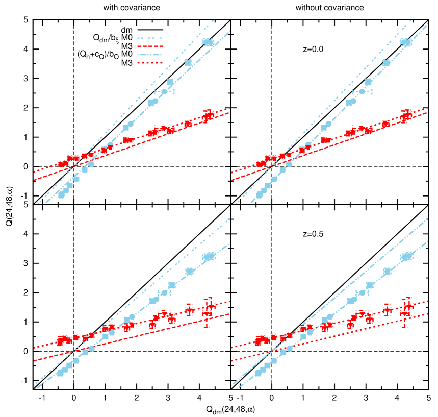
In Fig. 20 we also show examples for derived using smaller grid cell sizes and thinner shells to construct the triangles. These computations are more expensive than those based on larger grids cells, but closer to the theoretical picture. We find that the bias values change in most cases by around percent. These changes can be driven by changes in the amplitude of , but also by changes of the covariance matrix. Especially for high mass samples and at large scales and higher redshift the amplitude of becomes more noisy, which can result in larger values in the fit. The covariance becomes more diagonal since for smaller grid cells the different triangle opening angles are more independent of each other.
| Fig. | |||||||
|---|---|---|---|---|---|---|---|
| Mpc | Mpc | Mpc | |||||
| 5, 6, 7, 20 | |||||||
| 7, 20 | |||||||
| 6, 7, 11, 12, 17, 18, 19, 20 | |||||||
| 5, 20 | |||||||
| 7, 20 | |||||||
| 20 | |||||||
| 7, 20 | |||||||
| 20 |
