Causal Diagrams for Interference

Abstract

The term “interference” has been used to describe any setting in which one subject’s exposure may affect another subject’s outcome. We use causal diagrams to distinguish among three causal mechanisms that give rise to interference. The first causal mechanism by which interference can operate is a direct causal effect of one individual’s treatment on another individual’s outcome; we call this direct interference. Interference by contagion is present when one individual’s outcome may affect the outcomes of other individuals with whom he comes into contact. Then giving treatment to the first individual could have an indirect effect on others through the treated individual’s outcome. The third pathway by which interference may operate is allocational interference. Treatment in this case allocates individuals to groups; through interactions within a group, individuals may affect one another’s outcomes in any number of ways. In many settings, more than one type of interference will be present simultaneously. The causal effects of interest differ according to which types of interference are present, as do the conditions under which causal effects are identifiable. Using causal diagrams for interference, we describe these differences, give criteria for the identification of important causal effects, and discuss applications to infectious diseases.

FLA

and

Traditionally, causal inference has relied on the assumption of no interference, that is, the assumption that any subject’s outcome depends only on his own treatment and not on the treatment of any other subject. This assumption is often implausible; for example, it is violated when the outcome is an infectious disease and treating one individual may have a protective effect on others in the population. Recent work in statistics has focused on relaxing the assumption of no interference (Graham, Imbens and Ridder, 2010; Halloran and Struchiner, 1995; Hudgens and Halloran, 2008; Manski, 2013; Rosenbaum, 2007; Tchetgen Tchetgen and VanderWeele, 2012; Vansteelandt, 2007). Much of this work has been motivated by the study of infectious diseases (Halloran and Struchiner, 1995; Tchetgen Tchetgen and VanderWeele, 2012; VanderWeele and Tchetgen Tchetgen, 2011a, 2011b; Halloran and Hudgens, 2012). Researchers have also explored the implications of interference on residents of neighborhoods when some residents are given housing vouchers to move (Sobel, 2006) or when new resources are introduced to the neighborhood (VanderWeele, 2010). Others have written about the interference that arises from assigning children to classrooms and assigning classrooms to educational interventions (Graham, Imbens and Ridder, 2010; Hong and Raudenbush, 2008; VanderWeele et al., 2013). The rising prominence of social networks in public health research underscores the need for methods that take into account the interconnections among individuals’ treatments and outcomes (Christakis and Fowler, 2007; Cohen-Cole and Fletcher, 2008; Mulvaney-Day and Womack, 2009).

Graphical models have shed light on the identification of causal effects in many settings (Dahlhaus and Eichler, 2003; Didelez, Kreiner and Keiding, 2010; Freedman, 2004; Greenland, Pearl and Robins, 1999; Pearl, 1995, 1997, 2000; Robins, 2003; Tian and Pearl, 2002a; Vansteelandt, 2007) but have not yet been applied to settings with interference. In this paper, we describe how to draw causal diagrams representing the complex interdependencies among individuals in the presence of interference, and how to use those diagrams to determine what variables must be measured in order to identify different causal effects of interest. We review the literature on causal diagrams and identification of causal effects in the absence of interference in Section 1, and recent work on the estimation of causal effects in the presence of interference in Section 2. In Section 3, we discuss which covariates must be measured and controlled for in order to identify causal effects in the presence of interference. Section 4 introduces the three distinct types of interference, provides causal diagrams to help explicate their structure, and describes some of the causal effects we would wish to estimate and the assumptions required to identify them. In Section 5, we use the concepts introduced in Section 4 to elucidate the nature of interference in social networks. Section 6 concludes the paper.

1 Review of Identification of Causal Effects in the Absence of Interference

Suppose that we wish to estimate the average causal effect of a treatment $A$ on an outcome $Y$ from observational data on $n$ individuals for whom we have also measured a vector of confounders $C$. For simplicity, we will assume in this section and the next that $A$ is binary and $Y$ is continuous, but our remarks apply equally to $A$ and $Y$ discrete or continuous. Under the assumptions of no interference and a single version of treatment (we will not discuss the latter assumption here; see VanderWeele and Hernan, 2013, for discussion), $Y_{i}(a),a=0,1$ is defined as the counterfactual outcome we would have observed if, possibly contrary to fact, subject $i$ had received treatment $a$. The average causal effect of $A$ on $Y$ is equal to $E[Y(1)]-E[Y(0)]$, and it is identified under the three additional assumptions of consistency,

$$Y_{i}(a)=Y_{i}\quad\mbox{if }A_{i}=a,$$ (1)

conditional exchangeability,

$$Y_{i}(a)\amalg A_{i}|C_{i},$$ (2)

and positivity,

$$P(A_{i}=a|C_{i}=c)>0$$

$$\hphantom{\hskip 21.0pt}\mbox{for all }a\mbox{ in the support of }A\mbox{ and for all }c$$ (3)

$$\hphantom{\hskip 21.0pt}\mbox{in the support of }C\mbox{ such that }P(C=c)>0.$$

We refer the reader to Hernán and Robins (2006) for discussion of these assumptions.

The conditional exchangeability assumption is sometimes referred to as the “no unmeasured confounding assumption.” Identifying the variables that must be included in $C$ can be assessed with the aid of causal diagrams (e.g., Greenland and Robins, 1986; Greenland, Pearl and Robins, 1999; Pearl, 2003).

Causal diagrams, or causal directed acyclic graphs (DAGs) consist of nodes, representing the variables in a study, and arrows, representing causal effects. In a slight abuse of terminology, we will not distinguish between nodes on a DAG and the variables they represent. A DAG is a collection of nodes and arrows in which no variable is connected to itself by a sequence of arrows aligned head-to-tail. A causal DAG is a DAG on which arrows represent causal effects and that includes all common causes of any pair of variables on the graph. The causal DAG in Figure 1 represents the scenario in which the effect of $A$ on $Y$ is confounded by a single confounder $C$. The three arrows encode the causal effects of $C$ on $A$, $C$ on $Y$, and $A$ on $Y$. We briefly introduce terminology and results for DAGs but refer the reader to Pearl (2000, 2003) for details and discussion. Recently, Richardson and Robins (2013) introduced a new class of causal diagrams called single world intervention graphs (SWIGs). This work can be immediately and fruitfully applied to the interference settings we discuss below; however, in the interest of space we restrict our attention to DAGs.

Figure 1:

A path on a DAG is any unbroken, nonrepeating sequence of arrows connecting one variable to another. A directed path (or a causal path on a causal DAG) is a path that follows arrows from tail to head. A variable $X$ is an ancestor (or cause, if the DAG is causal) of $Z$ if there is a directed path from $X$ to $Z$. Equivalently, $Z$ is a descendent of $X$. If the directed path from $X$ to $Z$ consists of a single arrow, then $X$ is a parent of $Z$ and $Z$ is a child of $X$. On a causal DAG, we would say that $X$ has a direct effect on $Z$. If a path includes $X$, $W$ and $Z$ and if there are arrows from both $X$ and $Z$ into $W$, then $W$ is a collider on the path. A collider is a path-specific concept. For example, in Figure 1, $Y$ is a collider on one path from $C$ to $A$ (the path $C\rightarrow Y\leftarrow A$) but not on another (the path $C\rightarrow A\rightarrow Y$). A path can be unblocked, meaning roughly that information can flow from one end to the other, or blocked, meaning roughly that the flow of information is interrupted at some point along the path. If all paths between two variables are blocked, then the variables are $d$-separated, and if two variables are d-separated on a causal DAG then they are statistically independent. A path is blocked if there is a collider on the path such that neither the collider itself nor any of its descendants is conditioned on. An unblocked path can be blocked by conditioning on any noncollider along the path. Two variables are d-separated by a set of variables if conditioning on the variables in the set suffices to block all paths between them, and if two variables are d-separated by a third variable or a set of variables then they are independent conditional on the third variable or set of variables (Pearl, 1995, 2000).

A backdoor path from $X$ to $Z$ is one that begins with an arrow pointing into, rather than out of, $X$. For example, the path $A\leftarrow C\rightarrow Y$ in Figure 1 is a backdoor path from $A$ to $Y$. Pearl (1995) proved that conditioning on a set of nondescendants of $A$ that block all backdoor paths from $A$ to $Y$ suffices for exchangeability to hold for the effect of $A$ on $Y$. This set need not be unique.

Figure 2:

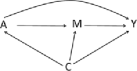
Identification of effects, other than total effects, often requires assumptions beyond (1), (2), and (1). Path-specific effects quantify the causal effect of one variable on another via specific causal pathways. Consider the DAG in Figure 2, which adds a mediator $M$ to the path from $A$ to $Y$. Now there are two different causal pathways from $A$ to $Y$, namely $A\rightarrow Y$ and $A\rightarrow M\rightarrow Y$. Causal effects of the form $E[Y(a)]-E[Y(a^{\prime})]$ capture all causal pathways from $A$ to $Y$ without distinguishing among them, but we may be interested specifically in direct effects, which bypass the mediator, and indirect effects, which go through the mediator. Define $M_{i}(a)$ to be the counterfactual value we would have observed for $M_{i}$ if $A_{i}$ had been set to $a$, and $Y_{i}(a,m)$ to be the counterfactual value of $Y_{i}$ that we would have observed if $M_{i}$ had been set to $m$ and $A_{i}$ to $a$. We make the additional consistency assumptions that $M_{i}(a)=M_{i}$ when $A_{i}=a$, that $Y_{i}(a,m)=Y_{i}$ when $A_{i}=a$ and $M_{i}=m$, and that $Y_{i}(a,M_{i}(a))=Y_{i}(a)$. Then the natural direct effect is defined as $E[Y(a,M(a))]-E[Y(a^{\prime},M(a))]$; it measures the expected change in $Y$ due to a change in $A$, holding $M$ fixed at $M(a)$. A direct path from $X$ to $Z$ is said to be deactivated in a particular causal contrast if $X$ is set to the same value in the counterfactual for $Z$ in both terms of the contrast. A path is deactivated if any arrow on the path is deactivated. In the natural direct effect, $A$ is set to the same value in the counterfactual for $M$ in both terms of the contrast; therefore the natural direct effect can be conceptualized as the effect of $A$ on $Y$ with the path $A\rightarrow M$ deactivated (Pearl, 2001). The natural indirect effect, defined as $E[Y(a^{\prime},M(a))]-E[Y(a^{\prime},M(a^{\prime}))]$, measures the expected change in $Y$ when $A$ is held fixed but $M$ changes from $M(a)$ to $M(a^{\prime})$. This is the effect of $A$ on $Y$ with the arrow from $A$ to $Y$ deactivated ($A$ is set to $a^{\prime}$ in the counterfactual for $Y$ in both terms of the contrast). The natural direct and indirect effects sum to the total effect of $A$ on $Y$: $E[Y(a)]-E[Y(a^{\prime})]=E[Y(a,M(a))]-E[Y(a^{\prime},M(a^{\prime})]=\{E[Y(a,M(a))]-E[Y(a^{\prime},M(a))]\}+\{E[Y(a^{\prime},M(a))]-E[Y(a^{\prime},\break M(a^{\prime}))]\}$. The controlled direct effect of $A$ on $Y$, given by $E[Y(a,m)]-E[Y(a^{\prime},m)]$ fixes $M$ at a specific value $m$ and compares the counterfactual outcomes under two different values of $A$. This is the effect of $A$ on $Y$ with the path $M\rightarrow Y$ deactivated.

In order to identify the controlled direct effect, the following assumptions are sufficient:

$$Y_{i}(a,m)\amalg A_{i}|C_{i}$$ (4)

and

$$Y_{i}(a,m)\amalg M_{i}|A_{i},C_{i}.$$ (5)

These correspond respectively to the absence of unblocked backdoor paths from $A_{i}$ to $Y_{i}$ (except possibly through $M_{i}$) conditional on $C_{i}$ and from $M_{i}$ to $Y_{i}$ conditional on $A_{i}$ and $C_{i}$. Avin, Shpitser and Pearl (2005) proved that in most settings the following is a necessary assumption for the identification of the average natural direct and indirect effects of $A_{i}$ on $Y_{i}$ mediated by $M_{i}$: there is no variable $W_{i}$ such that (i) there is an activated directed path from $A_{i}$ to $W_{i}$, (ii) there is a deactivated directed path from $W_{i}$ to $Y_{i}$ and (iii) there is an activated directed path from $W_{i}$ to $Y_{i}$. A variable that satisfies conditions (i), (ii) and (iii) is known as a recanting witness, and we call the assumption of no variable satisfying these conditions the recanting witness criterion. In the context of natural direct and indirect effects, the recanting witness criterion is met if there is no confounder of the mediator–outcome relation that is caused by treatment, or (Pearl, 2001)

$$Y_{i}(a,m)\amalg M_{i}\bigl{(}a^{\prime}\bigr{)}|C_{i}.$$ (6)

Assumptions (5), (4), (6) and

$$M_{i}(a)\amalg A_{i}|C_{i},$$ (7)

that is, the absence of unblocked backdoor paths from $A_{i}$ to $M_{i}$ conditional on $C_{i}$, suffice to identify the natural direct and indirect effects.

2 Review of Identification of Causal Effects in the Presence of Interference

Interference is present when one subject’s outcome may depend on other subjects’ treatments (Rosenbaum, 2007). It is often reasonable to make a partial interference assumption that interference can only occur within subgroups or blocks of subjects. This may be justified if the blocks are separated by time or space (Hudgens and Halloran, 2008; Sobel, 2006; Tchetgen Tchetgen and VanderWeele, 2012; Rosenbaum, 2007). Under interference, $Y_{i}(a)$ is not well-defined, since the value of $Y$ that would have been observed for subject $i$ had he received treatment $a$ may depend on the treatments received by other subjects. We define counterfactual notation for interference following Hudgens and Halloran (2008), Tchetgen Tchetgen and VanderWeele (2012), Rubin (1990) and Halloran and Struchiner (1995). Suppose that $n$ individuals fall into $N$ blocks, indexed by $k$, with $m=n/N$ individuals in each block. If $N=1$, so that interference may occur between any two subjects in the population, then we say that there is full interference. If $N=n$, then an individual’s treatment can only affect his own outcome and there is no interference. Let $\mathbf{A}_{k}\equiv(A_{k1},\ldots,A_{km})$ be the vector of treatment assignments for individuals in block $k$ and let $\mathbf{a}_{k}$ denote an $m$-dimensional vector in the support of $\mathbf{A}_{k}$. Let $\mathbf{Y}_{k}\equiv(Y_{k1},\ldots,Y_{km})$ and $\mathbf{C}_{k}\equiv(C_{k1},\ldots,C_{km})$ be the vector of outcomes and array of covariates, respectively, for individuals in block $k$. In what follows, we reserve boldface letters for vectors or arrays of length $m$ in which the $i$th entry corresponds to the $i$th individual in block $k$, and we omit the subscript $k$ when taking expectations over blocks. Define $Y_{ki}(\mathbf{a}_{k})$ to be the counterfactual outcome that we would have observed for individual $i$ in block $k$ under an intervention that set $\mathbf{A}_{k}$ to $\mathbf{a}_{k}$. Following Tchetgen Tchetgen and VanderWeele (2012) we replace assumption (1) above with a new assumption of consistency under interference:

$$Y_{ki}(\mathbf{a}_{k})=Y_{ki}\quad\mbox{when }\mathbf{A}_{k}=\mathbf{a}_{k}.$$ (8)

We also require modified positivity and exchangeability assumptions in order to identify causal effects under interference: we assume that we have measured a set of pretreatment covariates $C$ for each individual such that (Tchetgen Tchetgen and VanderWeele, 2012)

$$Y_{ki}(\mathbf{a}_{k})\amalg\mathbf{A}_{k}|\mathbf{C}_{k}$$ (9)

and

$$P(\mathbf{A}_{k}=\mathbf{a}_{k}|\mathbf{C}_{k}=\mathbf{c}_{k})>0$$

$$\hskip 44.0pt\mbox{for all }\mathbf{a}_{k}\mbox{ in the support of }\mathbf{A}_{k}$$ (10)

$$\hskip 44.0pt\mbox{and for all $\mathbf{c}_{k}$ in the support of }\mathbf{C}_{k}.$$

These assumptions suffice to identify the expectations of counterfactuals of the form $Y_{ki}(\mathbf{a}_{k})$ whenever $\mathbf{a}_{k}$ is an instance of a well-defined intervention $\mathbf{a}$ and, therefore, to identify causal effects that are contrasts of such expectations. An intervention will be well-defined if it uniquely determines which subjects in block receive treatment. Well-defined interventions are possible, for example, if all blocks are of the same size, if the individuals in each block are distinguishable from one another, and if the individuals are ordered in the same way across blocks. Suppose interference occurs within blocks comprised of a father (subject 1), a mother (subject 2) and a child (subject 3). Then an intervention $(1,0,1)$ indicates that the father and child receive treatment but the mother does not. If the blocks are of different sizes or if there is no natural way to distinguish among the individuals in each block, some interventions may be well-defined under assumptions that the effects of treatment are the same for different members of the block and do not depend on the size of the block, for example, the intervention that assigns treatment to every individual in every block. We assume throughout that all interventions are well-defined. For simplicity, we assume that the blocks are of the same size and that there is a natural ordering of the subjects in each block, but most of our comments and results extend to more general settings. (In the absence of well-defined interventions, some causal effects can still be defined, identified and estimated under two-stage randomization; see Hudgens and Halloran, 2008; Vanderweele, Tchetgen and Halloran, 2012; VanderWeele and Tchetgen Tchetgen, 2011b; Halloran and Hudgens, 2012.)

In Section 3, we use graphical models to determine which variables must be included in the conditioning set in order for exchangeability to hold. This gives the identification criteria under interference for causal effects that are contrasts of expectations of counterfactuals of the form $Y_{ki}(\mathbf{a}_{k})$. Sometimes we may wish to identify path-specific effects; these require additional assumptions for identification that we discuss below.

In this paper, we focus on identification, rather than estimation, of causal effects. We merely note here that, for the purposes of estimation and inference, the effective sample size is $N$ and thus observation of multiple blocks may be required.

2.1 Causal Effects of $\mathbf{A}$ on $Y$

Although recognition of the fact that interference may occur in certain settings dates at least as far back as Ross (1916), it is only recently that progress has been made on identifying causal effects in the presence of interference. Halloran and Struchiner (1995) defined four effects that do not depend on understanding the mechanisms underlying interference and that are identifiable under assumptions (8), (9) and (2).

The overall effect of intervention $\mathbf{a}$ compared to intervention $\mathbf{a}^{\prime}$ on subject $i$ is defined as $\mathit{OE}_{i}(\mathbf{a},\mathbf{a}^{\prime})\equiv E[Y_{i}(\mathbf{a})]-E[Y_{i}(\mathbf{a}^{\prime})]$. We use the index $i$ to indicate that the expectations do not average over individuals within a block but rather over blocks for a particular individual $i$. For example, if the blocks are comprised of a father (subject 1), a mother (subject 2) and a child (subject 3), then $\mathit{OE}_{3}(\mathbf{a},\mathbf{a}^{\prime})=E[Y_{3}(\mathbf{a})]-E[Y_{3}(\mathbf{a}^{\prime})]$ is the overall effect on a child of intervention $\mathbf{a}$ compared to intervention $\mathbf{a}^{\prime}$. The average overall effect $\mathit{OE}(\mathbf{a},\mathbf{a}^{\prime})\equiv E[Y(\mathbf{a})]-E[Y(\mathbf{a}^{\prime})]$, where $E[Y(\mathbf{a})]\equiv\frac{1}{m}\sum_{i=1}^{m}E[Y_{i}(\mathbf{a})]$, averages over the empirical mean of the counterfactual outcomes for each block. The unit-level effect of treatment on subject $i$ fixes the treatment assignments for all subjects in each block except $i$, and compares the counterfactual outcomes for subject $i$ under two different treatment assignments. Let $\mathbf{a}_{k,-i}=(a_{k,1},\ldots,a_{k,i-1},a_{k,i+1},\ldots,a_{k,m})$ be a vector of length $m-1$ of treatment values for all subjects in block $k$ except for subject $i$. Then $\mathit{UE}_{i}(\mathbf{a};\tilde{a},\bar{a})\equiv E[Y_{i}(\mathbf{a}_{-i},\tilde{a})]-E[Y_{i}(\mathbf{a}_{-i},\bar{a})]$, where $Y_{ki}(\mathbf{a}_{k,-i},\tilde{a})$ is subject $i$’s counterfactual outcome under the intervention in which the subjects in block $k$ except for subject $i$ receive treatments $\mathbf{a}_{k,-i}$ and subject $i$ receives treatment $\tilde{a}$. The spillover effect of intervention $\mathbf{a}$ compared to intervention $\mathbf{a}^{\prime}$ on subject $i$ fixes $i$’s treatment level and compares his counterfactual outcomes under the two different interventions. That is, $\mathit{SE}_{i}(\mathbf{a},\mathbf{a}^{\prime};\tilde{a})\equiv E[Y_{i}(\mathbf{a}_{-i},\tilde{a})]-E[Y_{i}(\mathbf{a}_{-i}^{\prime},\tilde{a})]$. (The unit-level effect is often referred to as the direct effect and the spillover effect as the indirect effect of an intervention, but in order to avoid confusion with the direct effect for DAGs defined in Section 2 and the natural direct and indirect effects defined in Section 2.2, we will use different terminology. See Tchetgen Tchetgen and VanderWeele, 2012, and Vanderweele, Tchetgen and Halloran, 2012, for further discussion of terminology.) We can also average these effects over individuals within a block. The average unit-level effect is $\mathit{UE}(\mathbf{a};\tilde{a},\bar{a})\equiv E[Y(\mathbf{a}_{-},\tilde{a})]-E[Y(\mathbf{a}_{-},\bar{a})]$ and the average spillover effect is $\mathit{SE}(\mathbf{a},\mathbf{a}^{\prime};\tilde{a})\equiv E[Y(\mathbf{a}_{-},\tilde{a})]-E[Y(\mathbf{a}_{-}^{\prime},\tilde{a})]$, where $E[Y(\mathbf{a}_{-},\tilde{a})]\equiv\frac{1}{m}\sum_{i=1}^{m}E[Y_{i}(\mathbf{a}_{-i},\tilde{a})]$. The total effect compares an individual’s counterfactual at one treatment level in a block that receives one intervention to his counterfactual at a different treatment level in a block that receives the another intervention: $\mathit{TE}_{i}(\mathbf{a},\mathbf{a}^{\prime};\tilde{a},\bar{a})\equiv E[Y_{i}(\mathbf{a}_{-i},\tilde{a})]-E[Y_{i}(\mathbf{a}_{-i}^{\prime},\bar{a})]$. The average total effect is defined analogously to the other average effects above. Hudgens and Halloran (2008) showed that the total effect can be decomposed into a sum of unit-level and spillover effects: $\mathit{TE}_{i}(\mathbf{a},\mathbf{a}^{\prime};\tilde{a},\bar{a})=E[Y_{i}(\mathbf{a}_{-i},\tilde{a})]-E[Y_{i}(\mathbf{a}_{-i},\bar{a})]+E[Y_{i}(\mathbf{a}_{-i},\bar{a})]-E[Y_{i}(\mathbf{a}_{-i}^{\prime},\bar{a})]=\mathit{DE}_{i}(\mathbf{a};\break\tilde{a},\bar{a})+\mathit{IE}_{i}(\mathbf{a},\mathbf{a}^{\prime};\bar{a})$.

Sobel (2006), Hudgens and Halloran (2008), VanderWeele and Tchetgen Tchetgen (2011b) and Tchetgen Tchetgen and VanderWeele (2012) proposed ways to estimate and extend unit-level, spillover, total and overall effects. We will not discuss these extensions here except to note that they require the same three identifying assumptions (8), (9) and (2).

2.2 Path Specific Effects of $\mathbf{A}$ on $Y$

In Sections 4.2 and 4.3, we describe path-specific effects that may be of interest in certain interference contexts; here we review and extend the literature on path-specific effects under interference. Let $\mathbf{M}_{k}\equiv(M_{k1},\ldots,M_{km})$ be a vector of variables that may lie on a causal pathway from $\mathbf{A}_{k}$ to $Y_{ki}$. VanderWeele (2010) provided identifying assumptions and expressions for mediated effects with cluster-level treatments. These effects are applicable to the context of partial interference where there is interference by the mediator but not by the treatment ($M_{ki}$ may have an effect on $Y_{kj}$ for $i\neq j$, but $\mathbf{A}_{k}$ is set at the cluster level, and thus is the same for all individuals in block $k$). We adapt them here to accommodate interference by the treatment in addition to the mediator. We make the consistency assumptions that $\mathbf{M}_{k}(\mathbf{a}_{k})=\mathbf{M}_{k}$ when $\mathbf{A}_{k}=\mathbf{a}_{k}$, that $Y_{kj}(\mathbf{a}_{k},\mathbf{m}_{k})=Y_{kj}$ when $\mathbf{A}_{k}=\mathbf{a}_{k}$ and $\mathbf{M}_{k}=\mathbf{m}_{k}$, and that $Y_{kj}(\mathbf{a}_{k},\mathbf{M}_{k}(\mathbf{a}_{k}))=Y_{kj}(\mathbf{a}_{k})$. The expected controlled direct effect of a block-level treatment $\mathbf{A}_{k}$ on individual $i$’s outcome, not through $\mathbf{M}_{k}$, is defined as $E[Y_{i}(\mathbf{a},\mathbf{m})]-E[Y_{i}(\mathbf{a}^{\prime},\mathbf{m})]$; it measures the expected change in $Y_{ki}$ due to a change in $\mathbf{A}_{k}$, intervening to set $\mathbf{M}_{k}$ to $\mathbf{m}_{k}$. The expected natural direct effect is $E[Y_{i}(\mathbf{a},\mathbf{M}(\mathbf{a}))]-E[Y_{i}(\mathbf{a}^{\prime},\mathbf{M}(\mathbf{a}))]$; it measures the expected change in $Y_{ki}$ due to a change in $\mathbf{A}_{k}$, holding $\mathbf{M}_{k}$ fixed at $\mathbf{M}_{k}(\mathbf{a}_{k})$. The expected natural indirect effect of $\mathbf{A}_{k}$ on $Y_{ki}$ through $\mathbf{M}_{k}$, given by $E[Y_{i}(\mathbf{a}^{\prime},\mathbf{M}(\mathbf{a}))]-E[Y_{i}(\mathbf{a}^{\prime},\mathbf{M}(\mathbf{a}^{\prime}))]$, measures the expected change in $Y_{ki}$ when $\mathbf{A}_{k}$ is fixed but $\mathbf{M}_{k}$ changes from $\mathbf{M}_{k}(\mathbf{a}_{k})$ to $\mathbf{M}_{k}(\mathbf{a}_{k}^{\prime})$. Average controlled direct, natural direct, and natural indirect effects are defined similarly to the average effects in Section 2.1: we average the counterfactuals within each block before taking the expectations over blocks. These natural direct and indirect effects are identifiable under the following four assumptions:

$$Y_{ki}(\mathbf{a}_{k},\mathbf{m}_{k}) \amalg \mathbf{A}_{k}|\mathbf{C}_{k},$$ (11)

$$Y_{ki}(\mathbf{a}_{k},\mathbf{m}_{k}) \amalg \mathbf{M}_{k}|\mathbf{A}_{k},\mathbf{C}_{k},$$ (12)

$$\mathbf{M}_{k}(\mathbf{a}_{k}) \amalg \mathbf{A}_{k}|\mathbf{C}_{k}$$ (13)

and

$$Y_{ki}(\mathbf{a}_{k},\mathbf{m}_{k})\amalg\mathbf{M}_{k}\bigl{(}\mathbf{a}_{k}^{\prime}\bigr{)}|\mathbf{C}_{k}.$$ (14)

Assumptions (11), (12) and (13) correspond, respectively, to the absence of unblocked backdoor paths from $\mathbf{A}_{k}$ to $Y_{ki}$ (except possibly through $\mathbf{M}_{k}$) conditional on $\mathbf{C}_{k}$, from $\mathbf{M}_{k}$ to $Y_{ki}$ conditional on $\mathbf{A}_{k}$ and $\mathbf{C}_{k}$, and from $\mathbf{A}_{k}$ to $\mathbf{M}_{k}$ conditional on $\mathbf{C}_{k}$. Assumption (14), similar to (6), corresponds to the recanting witness criterion. Under these assumptions, counterfactual expectations of the form $E[Y_{i}(\mathbf{a}^{\prime},\mathbf{M}(\mathbf{a}))]$ are identified and, therefore, so are the natural direct and indirect effects, which are contrasts of such expectations. Specifically, $E[Y_{i}(\mathbf{a}^{\prime},\mathbf{M}(\mathbf{a}))]$ is identified by

$$\sum_{\mathbf{c}}\sum_{\mathbf{m}}E\bigl{[}Y_{i}|\mathbf{A}=\mathbf{a}^{\prime},\mathbf{M}=\mathbf{m},\mathbf{C}=\mathbf{c}\bigr{]}$$

$$\hphantom{\sum_{\mathbf{c}}\sum_{\mathbf{m}}}{}\cdot P(\mathbf{M}=\mathbf{m}|\mathbf{A}=\mathbf{a},\mathbf{C}=\mathbf{c})P(\mathbf{C}=\mathbf{c}).$$

Assumptions (11) and (12) suffice to identify the controlled direct effect.

3 Covariate Control

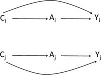
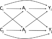
Although the subscripts are usually suppressed, under the assumption of no interference the standard DAG for the effect of a treatment $A$ on an outcome $Y$ with confounders $C$ is drawn to show the relationships among $Y_{i}$, $A_{i}$ and $C_{i}$ for subject $i$. Under interference, however, it is not sufficient to consider causal pathways at the individual level; a causal DAG must depict an entire block. For simplicity, we will focus on blocks of the smallest size that preserves the essential structure of interference, which for our purposes will be two or three. The principles extend to groups of any size, but the DAGs become considerably more complex as the blocks grow. The DAG for the effect of $A$ on $Y$ in a group of size two with no interference is depicted in Figure 3. In what follows, we represent a single block of subjects on each DAG, and we therefore suppress the subscript $k$ indicating membership in block $k$.

Figure 3:

Figure 4:

(a)	(b)	(c)
(d)	(e)	(f)
(g)

Figure 5:

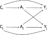
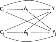
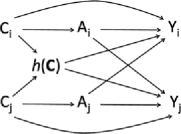
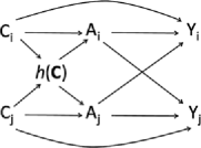
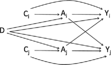
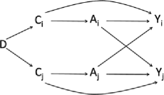
Interference can be represented by a DAG like the one given in Figure 4. The arrows from $A_{i}$ to $Y_{j}$ for $i\neq j$ represent the effect that one individual’s treatment has on another’s outcome. This representation suffices whenever contrasts of counterfactuals of the form $Y(\mathbf{a})$, such as the effects described in Section 2.1, are the only effects of interest. However, as we will see below, when contagion or allocational interference are present, such a diagram does not represent information about how the effect of $A_{i}$ on $Y_{j}$ operates. In Section 4, we describe how to represent this additional information on a DAG. We describe covariate control in the general cases depicted in the DAGs in Figures 4 and 5 before moving on in Section 4 to tease apart the structures that make direct interference, interference by contagion, and allocational interference distinct. The principles of covariate control in the presence of interference are straightforward: like in the case of no interference, they follow from the fact that all backdoor paths from treatment to outcome must be blocked by a measured set of covariates. However, without taking the time to draw the operative causal DAG with interference it is easy to make mistakes, like controlling only for individual-level covariates when block-level covariates are necessary to identify the causal effect of interest. Below we will consider a number of different settings and causal structures, and discuss in each whether control for only an individual’s covariates suffices to identify causal effects or whether control for the covariates of the entire block (or of some summary) is needed.

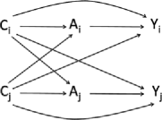
If the individuals in the block share no common causes of $A$ or $Y$, as in the DAG in Figure 4, then $C_{i}$ suffices to block the backdoor paths from $A_{i}$ to $Y_{i}$ and from $A_{j}$ to $Y_{i}$ and, therefore, exchangeability for the effect of $\mathbf{A}$ on $Y_{i}$ holds conditional on $C_{i}$. That is, $Y_{i}(a_{i},a_{j})\amalg\mathbf{A}|C_{i}$ for all $i$. If $C_{j}$ is a direct cause of $Y_{i}$ for $i\neq j$, as in Figure 5(a), then exchangeability for the effect of $\mathbf{A}$ on $Y_{i}$ necessitates block- and not just individual-level covariates. Even if each individual’s treatment is randomized conditional on his own covariates (this corresponds to the absence of arrows $C_{j}$ to $A_{i}$ for $i\neq j$ on the DAG), there is still a backdoor path from $A_{j}$ to $Y_{i}$ via $C_{j}$ and, somewhat counterintuitively, it is necessary to control for $C_{j}$ in addition to $C_{i}$ in any model for the effect of $\mathbf{A}$ on $Y_{i}$. On the other hand, if $C_{j}$ directly affects $A_{i}$ but not $Y_{i}$ for $i\neq j$, as in Figure 5(b), then for exchangeability for the effect of $\mathbf{A}$ on $Y_{i}$ it suffices to condition only on $C_{i}$. If, in addition to $C_{i}$, a function $h(\mathbf{C})$ of the vector of covariates influences outcome (Figure 5(c); for example, the mean value of $\mathbf{C}$ for the block), then $C_{i}$ and either $h(\mathbf{C})$ or $C_{j}$ need to be conditioned on in order to achieve exchangeability for the effect of $\mathbf{A}$ on $Y_{i}$. If $h(\mathbf{C})$ only influences treatment assignment (Figure 5(d)), then only $C_{i}$ must be conditioned on. If a block-level characteristic $D$ is a common cause of $A$ and $Y$ (Figure 5(e)), then $C_{i}$ and $D$ must be conditioned on in order to achieve exchangeability for the effect of $\mathbf{A}$ on $Y_{i}$. If $C_{i}$ and $C_{j}$ share a common cause (Figure 5(f)), then exchangeability for the effect of $\mathbf{A}$ on $Y_{i}$ holds conditional on $C_{i}$.

Even in the absence of interference for the effect of $\mathbf{A}$ on $\mathbf{Y}$, there are scenarios in which individual-level covariates do not suffice to control for the effect of an individual’s treatment on his own outcome. For example, the DAG in Figure 5(g) depicts a scenario in which one individual’s covariates affect another individual’s treatment and outcome (represented by the arrows $C_{i}\rightarrow A_{j}$ and $C_{i}\rightarrow Y_{j}$), but there is no effect of one individual’s treatment on another’s outcome (no directed path from $A_{i}$ to $Y_{j}$). In other words, there is interference for the effect of $\mathbf{C}$ on $\mathbf{Y}$ but not for the effect of $\mathbf{A}$ on $\mathbf{Y}$. Vansteelandt (2007) noted that in this setting it is necessary to condition on $\mathbf{C}$ to achieve exchangeability for the effect of $A_{i}$ on $Y_{i}$.

Consider the DAG in Figure 4, but now suppose that $\mathbf{C}$ is unobserved. As we discussed above, $C_{i}$ is a confounder of the effect of $A_{i}$ on $Y_{i}$, but in this DAG the effect of $A_{j}$ on $Y_{i}$ is unconfounded (there is no backdoor path from $A_{j}$ to $Y_{i}$). If a researcher hypothesizes that the DAG in Figure 4 represents the underlying causal structure in a particular setting but he does not have access to data on the confounders $\mathbf{C}$, then the effect of $\mathbf{A}$ on $Y_{i}$ is not identified. However, the unconfounded effect of $A_{j}$ on $Y_{i}$ is identified by $E[Y_{i}|A_{j}=a_{j}]$. This quantity has an interpretation in the interference setting as the weighted average of expected counterfactuals within strata of $C$.

$$E[Y_{i}|A_{j}=a_{j}]$$

$$\quad=\sum_{a_{i}}\sum_{c}E[Y_{i}|A_{i}=a_{i},A_{j}=a_{j},C_{i}=c]$$

$$\hphantom{\quad=\sum_{a_{i}}\sum_{c}}{}\cdot P(A_{i}=a_{i}|C_{i}=c)P(C_{i}=c)$$

$$\quad=\sum_{a_{i}}\sum_{c}E\bigl{[}Y_{i}(a_{i},a_{j})|A_{i}=a_{i},A_{j}=a_{j},C_{i}=c\bigr{]}$$

$$\hphantom{\quad=\sum_{a_{i}}\sum_{c}}{}\cdot P(A_{i}=a_{i}|C_{i}=c)P(C_{i}=c)$$

$$\quad=\sum_{a_{i}}\sum_{c}E\bigl{[}Y_{i}(a_{i},a_{j})|C_{i}=c\bigr{]}$$

$$\hphantom{\quad=\sum_{a_{i}}\sum_{c}}{}\cdot P(A_{i}=a_{i}|C_{i}=c)P(C_{i}=c),$$

where the first equality relies on the facts that $A_{i}\amalg A_{j}|C_{i}$ and $C_{i}\amalg A_{j}$, the second relies on consistency, and the third on conditional exchangeability. Alternatively, this quantity has the interpretation of $E[Y_{i}(a_{j})]$ in an experiment where $Y_{i}$ is considered to be the only outcome, $A_{j}$ is the treatment of interest and is intervened on, and $A_{i}$ is randomly assigned according to the actual distribution $P(A_{i}|C_{i})$ in the population.

The hypothetical experiment described above points toward a possible strategy for estimating the effect of one component of $\mathbf{A}$ on $Y_{i}$ when the confounders of the effect of $\mathbf{A}$ on $Y_{i}$ are not fully observed. The researcher can analyze each block of subjects as a single observation, with a single treatment and outcome. This strategy discards data on others’ treatments and outcomes but may allow for progress even if the full set of covariates needed to identify $Y_{i}(\mathbf{a})$ are not observed.

In some of the DAGs in Figure 5, identification of the effect of $A_{j}$ on $Y_{i}$ requires fewer covariates than the effect of $\mathbf{A}$ on $Y_{i}$. In Figure 5(c), $C_{j}$ suffices to control for confounding of the effect of $A_{j}$ on $Y_{i}$ even though it does not suffice for the effect of $\mathbf{A}$ on $Y_{i}$. For the DAG in Figure 5(e), $D$ suffices to control for confounding of the effect of $A_{j}$ on $Y_{i}$.

In some cases, we can identify the effect of $A_{i}$ on $Y_{i}$ with fewer covariates than are required to identify the effect of $\mathbf{A}$ on $Y_{i}$. In Figures 5(a) and 5(c), we can identify the effect of $A_{i}$ on $Y_{i}$ if only $C_{i}$ is observed, even though we cannot identify the effect of $\mathbf{A}$ on $Y_{i}$ without also observing $C_{j}$ (or $h(\mathbf{C})$). In the Appendix, we give the identifying expressions for these effects.

For the DAGs in Figures 5(b)–5(f), the entire vector $\mathbf{C}$ is not necessary to identify the effect of $\mathbf{A}$ on $Y_{i}$, though it would in general be necessary in order to jointly identify the effects of $\mathbf{A}$ on $Y_{i}$ and on $Y_{j}$ (i.e., the effect of $\mathbf{A}$ on $\mathbf{Y}$). This is because in order to identify the effect of $\mathbf{A}$ on $\mathbf{Y}$ we require conditional exchangeability to hold for all subjects. In these settings, if $\mathbf{C}$ is not fully observed but certain components or functions of $\mathbf{C}$ required to identify the effect of $\mathbf{A}$ on $Y_{i}$ are, then we can proceed by considering $Y_{i}$ to be the only outcome in each block. We can still consider the full vector of treatments $\mathbf{A}$, and therefore identify unit-level, spillover, total and overall effects of $\mathbf{A}$ on $Y_{i}$.

4 Three Distinct Types of Interference

By understanding the causal mechanisms underlying interference, we can more precisely target effects of interest. There are three distinct causal pathways by which one individual’s treatment may affect another’s outcome. All fall under the rubric of interference. The distinction among them has generally not been made, but they differ in causal structure, effects of interest and requirements for identification of effects. Often more than one type of interference will be present simultaneously.

The first pathway by which interference may operate is a direct causal effect of one individual’s treatment on another individual’s outcome, unmediated with respect to the first individual’s outcome. We call this direct interference. As an example, suppose that the outcome is obesity and the treatment is dietary counseling from a nutritionist. An individual who receives treatment can in turn “treat” his associates by imparting to them the information gained from the nutritionist; therefore, if individual $i$ receives treatment and individual $j$ does not, individual $j$ may be nevertheless be exposed to the treatment of individual $i$ and his or her outcome will be affected accordingly.

A second pathway by which one individual’s treatment may affect another individual’s outcome is via the first individual’s outcome. For example, if the outcome is an infectious disease and the treatment is a prophylactic measure designed to prevent disease, then the treatment of individual $i$ may affect the outcome of individual $j$ by preventing individual $i$ from contracting the disease and thereby from passing it on. We call this type of interference interference by contagion. It is differentiated from direct interference by the fact that it does not represent a direct causal pathway from the exposed individual to another individual’s outcome, but rather a pathway mediated by the outcome of the exposed individual.

The third pathway for interference is allocational interference. Treatment in this setting allocates individuals to groups; through interactions within a group individuals’ characteristics may affect one another. An example that often arises in the social science literature is the allocation of children to schools or of children to classrooms within schools (Angrist and Lang, 2004; Graham, Imbens and Ridder, 2010; Hong and Raudenbush, 2008). The performance and behavior of student $i$ may affect the performance and behavior of student $j$ in the same class, for example, by distracting or motivating student $j$ or by occupying the teacher’s attention. Another example that can be seen as allocational interference is the effect of college enrollment on wage differences for college- versus high-school-educated workers, where the wage difference depends on the proportion of workers in each education category (Heckman, Lochner and Taber, 1998).

4.1 Direct Interference

Direct interference is present when there is a causal pathway from one individual’s treatment to another individual’s outcome, not mediated by the first individual’s outcome. Interference can be direct with respect to a particular outcome but not another. Consider two individuals living in the same household, each randomized to an intervention designed to prevent high cholesterol. Suppose the intervention consists of cooking classes, nutritional counseling and coupons that can be redeemed for fresh produce, and consider a household in which one individual is treated and one untreated. The treated individual could bring fresh produce into the household, prepare healthy meals, and talk about the nutritionist’s counsel, thereby exposing the other individual to a healthier diet. If the outcome of interest is a measure of blood cholesterol level, then this is an example direct interference: the untreated individual is exposed to the treated individual’s diet and that exposure reduces the untreated individual’s cholesterol. On the other hand, if the outcome is a measure of healthy diet and behavior, then the same story depicts contagion rather than direct interference: the treated individual adopts a healthier diet which results in the untreated individual also adopting a healthier diet. Diet may spread by contagion; cholesterol presumably would not.

In many settings, direct interference and contagion will be present simultaneously for the same outcome. For example, suppose that in the story above the outcome were weight change. Then it is possible that the treated individual’s family member could lose weight both because of exposure to healthier foods (direct interference) and because he was motivated by the weight loss of his relative (contagion).

Direct interference has the simplest causal structure of the three types of interference. In addition to a direct causal path from $A_{i}$ to $Y_{i}$, there is also a direct path from $A_{i}$ to $Y_{j}$ for all pairs $(i,j)$ such that subjects $i$ and $j$ are in the same block. Direct interference in a block of size two is depicted in the DAGs in Figures 4 and 5, with the exception of Figure 5(g). Because there is only a single path from $A_{i}$ to $Y_{j}$ for any pair $i,j$, differences between counterfactuals of the form $Y_{i}(\mathbf{a})$ capture all of the causal effects of $\mathbf{A}$ on $Y_{i}$ and, therefore, effects like the total, unit-level, spillover and overall effects described in Section 2.1 summarize the causal effects of $\mathbf{A}$ on $Y_{i}$.

4.2 Interference by Contagion

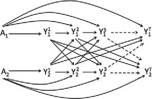
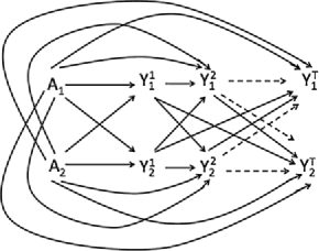
Interference by contagion often has a complex causal structure, because it can involve feedback among different individuals’ outcomes over time. The causal structure of the effect of $A_{i}$ on $Y_{i}$ is straightforward: $A_{i}$ has a direct protective effect on $Y_{i}$, represented by a direct arrow from $A_{i}$ to $Y_{i}$ on the DAG. The effect of $A_{i}$ on $Y_{j}$ is considerably more complex. It is tempting to represent the effect of $A_{i}$ on $Y_{j}$ as a mediated effect through $Y_{i}$, but this cannot be correct, as $Y_{i}$ and $Y_{j}$ are contemporaneous and, therefore, one cannot cause the other. The effect of $A_{i}$ on $Y_{j}$ is mediated through the evolution of the outcome of individual $i$; this complicated structure is depicted in the DAG in Figure 6, where $Y_{i}^{t}$ represents the outcome of individual $i$ at time $t$, $T$ is the time of the end of follow-up, and the dashed arrows represent times $4$ through $T-1$, which do not fit on the DAG (but which we assume were observed). The unit of time required to capture the causal structure depends on the nature of transmission of the outcome; it should be the case that the probability of one individual’s outcome affecting another’s is unaltered by differences in timing on a scale smaller than the units used.

Figure 6:

In order to further explicate the structure, we consider the case of an infectious disease like the flu. Infectious diseases are paradigmatic examples of contagion. Halloran and Struchiner (1995), Hudgens and Halloran (2008) and VanderWeele and Tchetgen Tchetgen (2011a) have written about identification and estimation of overall, unit-level, spillover and total effects for vaccinations against infectious diseases, and we follow up with this literature in Section 4.2.1. Although we illustrate the principles of interference by contagion through the lens of infectious diseases, this type of interference can occur in many and diverse settings: an educational intervention assigned to one student could affect that student’s performance, which in turn might affect the performance of her classmates; a get-out-the-vote mailing could motivate its recipients to decide to vote, and communicating that decision to friends could change the friends’ voting behavior. The principles that we discuss below apply to any of these settings.

Suppose that the flu vaccine has a protective effect against the flu by preventing or shortening the duration of episodes of the flu for some individuals. Let $A$ be an indicator of getting the flu vaccine before the start of a six-month long flu season, and let $Y$ be the total number of days spent infectious with the flu over the course of the season. In the DAG in Figure 6, $Y_{i}^{t}$ represents the flu status of individual $i$ at time $t$ (measured in days), $T\equiv 180$ is the day of the end of flu season, and the dashed arrows represent days $4$ through $T-1$, which do not fit on the DAG (but which we assume were observed). Let $Y_{i}^{t}$ be the total number of days spent infectious up to and including day $t$. (Note that, when $Y_{i}^{t}$ is observed for all $t$, this is equivalent to coding it as an indicator of individual $i$ being infectious at time $t$.) In choosing days as the unit of time, we are making the assumption that the probability of one individual infecting another is not affected by a difference of a fraction of a day in flu duration.

Figure 7:

We will rarely have fine-grained information on the evolution of the outcome over time. In the rest of this section, we describe how to draw the appropriate causal DAGs and how to identify causal effects in such cases. Drawing a causal DAG using only a subset of relevant variables has been extensively studied in the graphical models literature and involves an operation known as projection (Pearl and Verma, 1994; Tian and Pearl, 2002b; Verma, 1993). Projection algorithms are somewhat technical; below we provide an intuitive discussion of the construction of causal DAGs when not all variables relevant to contagion are observed.

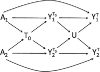
If we only observe the outcome (cumulative days of the flu) at the end of the season, then, as in the DAG in Figure 7, we replace the collection of all unobserved variables (i.e., $Y_{i}^{t}$ for $t<T$) with $U$. Without additional assumptions, we cannot replace the two diagonal pathways through $U$ with direct arrows from $A_{1}$ to $Y_{2}^{T}$ and from $A_{2}$ to $Y_{1}^{T}$; that would imply that $Y_{1}^{T}\amalg Y_{2}^{T}|A_{1},A_{2}$, which is shown to be false by the DAG in Figure 6. If we know who gets the flu first, then the DAG in Figure 8 represents the causal relations among the observed variables, where $T_{0}$ is the time of the first case of the flu. The unmeasured variable $U$ cannot be omitted because $Y_{1}^{T}$ is not independent of $Y_{2}^{T}$ conditional on $\{Y_{1}^{T_{0}},Y_{2}^{T_{0}}\}$; $Y_{1}^{T}$ depends on the number and timing of individual 2’s illnesses between time $T_{0}$ and time $T$. It might seem as though $Y_{1}^{T_{0}}$ should be independent of $Y_{2}^{T_{0}}$ conditional on $\{A_{1},A_{2}\}$ in this scenario, because there can be no contagion before the first case of the flu. But this is not the case: $Y_{i}^{T_{0}}$ can be thought of as an indicator that individual $i$ gets the flu before or at the same time as individual $j$, and this is dependent on individual $j$ remaining healthy through time $T_{0}-1$. On the other hand, conditioning on the time of the first case of the flu renders $Y_{1}^{T_{0}}$ and $Y_{2}^{T_{0}}$ independent, because conditioning on $T_{0}$ is tantamount to conditioning on both individuals remaining healthy until the time of the first case, that is, on their entire flu histories up to time $T_{0}$.

Figure 8:

Suppose information on the number but not duration of cases of the flu is available. Then we could define $Y^{t}$ to be the number of distinct cases initiated by time $t$. However, this outcome fails to capture all of the relevant information about an individual’s flu status, because a case of the flu that lasts ten days may be more contagious than one that lasts five days. Therefore, there may be an effect of $A_{i}$ on $Y_{j}^{t}$ that is not mediated by $Y_{j}^{s}$, $s<t$, being instead mediated by the duration of individual $i$’s flu incidents. This is represented on the DAG in Figure 9 by an arrow from $A_{i}$ to $Y_{j}^{t}$. These arrows encode the fact that $Y_{j}^{t}$ is dependent on $Y_{i}^{t}$ even conditional on $\{Y_{i}^{s},Y_{j}^{s}\}$ for all $s<t$. Similarly, if the outcome on the DAG in Figure 8 were the total number of flu episodes by the end of the season instead of the cumulative days of flu we would add arrows from $A_{i}$ to $Y_{j}^{T_{0}}$ and to $Y_{j}^{T}$.

Figure 9:

Figure 10:

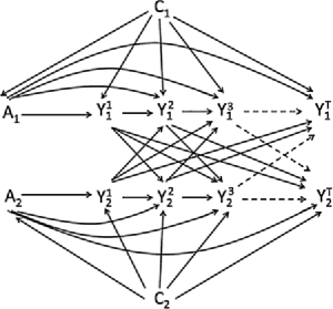
If there are common causes $C$ of treatment and outcome for each individual, as in the DAG in Figure 10, then exchangeability for the effect of $\mathbf{A}$ on $Y_{i}^{T}$ will hold conditional on $C_{i}$. If there are common causes of treatments for different individuals, or of treatments and outcomes across individuals, then exchangeability requires conditioning on them. The same conclusions about exchangeability hold if we observe the outcome only at select time points.

The overall, unit-level, spillover and total effects defined in Section 2.1 do not distinguish among the multiple distinct causal pathways from $A_{i}$ to $Y_{j}^{T}$. We discuss estimation of path-specific effects below.

4.2.1 Contagion and infectiousness

Recently, Vanderweele, Tchetgen and Halloran (2012) described the decomposition of the spillover effect, that is the effect of $A_{i}$ on $Y_{j}$, into a “contagion effect” and an “infectiousness effect.” The contagion effect is the protective effect that vaccinating one individual has on another’s disease status by preventing the vaccinated individual from getting the disease and thereby from transmitting it, similar to the effect we discussed above. In order to illustrate the infectiousness effect, consider the following refinement to our example. Suppose that a vaccine exists for the flu that prevents the disease for some individuals and also makes some cases of the disease among vaccinated individuals less likely to be transmitted. Let $A$ be an indicator of vaccination before the start of flu season and let $Y^{t}$ be the total number of episodes of flu up to and including day $t$. Then $A_{i}$ may have an effect on $Y_{j}^{t}$ even if it has no effect on $Y_{i}^{t}$, that is, even if individual $i$ would get the flu whether vaccinated or not, by preventing individual $i$ from transmitting the flu to individual $j$. This infectiousness effect represents a pathway that is distinct from the contagion effect because it does not operate through the infection status of the vaccinated individual. The infectiousness effect has the structure of a direct effect by which individual $i$’s vaccination confers improved protection against individual $i$’s flu on individual $j$; it represents a type of direct interference. This is similar to the example above in which the duration of flu episodes was unobserved: infectiousness, like flu duration, is a property of the infected individual’s disease state, but if it is not captured by the outcome measure then it has the structure of a direct effect of $A_{i}$ on $Y_{j}$. The contagion and infectiousness effects are not identifiable without strong assumptions or carefully conceived data collection. When they are identifiable their sum (or product if they are defined on the multiplicative scale) is equal to the total spillover effect of $A_{i}$ on $Y_{j}$.

Figure 11: This DAG corresponds to a household of size two in which individual 2 is always unvaccinated and disease status is assessed at the end of follow-up. $U$ represents unmeasured variables.

Figure 12: This DAG corresponds to the same setting as Figure 11, but under the assumptions that individual 2 can only be infected by individual 1 and that only one event is possible per subject during follow-up.

Vanderweele, Tchetgen and Halloran (2012) defined the contagion and infectiousness effects as the natural indirect and direct effects, respectively, of $A_{1}$ on $Y_{2}^{T}$ with $Y_{1}^{T_{0}}$ as the mediator, where $T_{0}$ is the day of the first flu infection and $T$ is the day of the end of follow-up, for example, the last day of the flu season. That is, the contagion effect is defined as $E[Y_{2}^{T}(0,Y_{1}^{T_{0}}(1))]-E[Y_{2}^{T}(0,Y_{1}^{T_{0}}(0))]$ and infectiousness by $E[Y_{2}^{T}(1,Y_{1}^{T_{0}}(1))]-E[Y_{2}^{T}(0,Y_{1}^{T_{0}}(1))]$. For simplicity and consistency with the existing literature we adopt the setting used in VanderWeele and Tchetgen Tchetgen (2011a), Vanderweele, Tchetgen and Halloran (2012) and Halloran and Hudgens (2012): each block is a group of size two who share a household, and in each pair individual 1 is randomized to vaccine while individual 2 is always unvaccinated. If, as those authors assumed, disease status is observed only at the end of follow-up, Figure 11 depicts the operative DAG. Although there is an unmeasured variable on the path from $A_{1}$ to $Y_{2}^{T}$, it is not a confounder and we can identify the effect of $A_{1}$ on $Y_{2}^{T}$. However, we cannot identify the component contagion and infectiousness effects without observing the mediator $Y_{1}^{T_{0}}$. In order to circumvent the problem of the unobserved mediator, Vanderweele, Tchetgen and Halloran (2012) assumed that each individual can be infected only once and that individual 2 can only be infected by individual 1, as would be the case if individual 2 were homebound. These assumptions dramatically simplify the causal structure by ensuring that individual 1 is infected first and that there is no feedback between the time of first infection and the end of follow up. Then $Y_{1}^{T}$ must be equal to $Y_{1}^{T_{0}}$, and thus $Y_{1}^{T_{0}}$ is observed. These assumptions are encoded by the DAG in Figure 12. Now the contagion and infectiousness effects can be identified as the natural indirect and direct effects of $A_{1}$ on $Y_{2}^{T}$ mediated by $Y_{1}^{T}=Y_{1}^{T_{0}}$, as long as assumptions (4) through (7) are met. Three of these assumptions correspond to the absence of any unmeasured confounding of the relationships between $A_{1}$ and $Y_{1}^{T}$, between $Y_{1}^{T}$ and $Y_{2}^{T}$ conditional on $A_{1}$, and between $A_{1}$ and $Y_{2}^{T}$, respectively. These assumptions can be made conditional on measured covariates $\mathbf{C}$. Assumption (6) is the recanting witness criterion.

Figure 13: This DAG corresponds to the same setting as Figure 12, but without the assumption that individual 2 can only be infected by individual 1. The dashed arrow is present when $T$ is defined as the end of the flu season; it is absent when $T$ is defined as $T_{0}+s$.

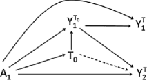
The simplifying assumption that the outcome can occur at most once may be reasonable for many infectious diseases. More limiting is the assumption that individual 2 can only be infected by individual 1. Here, we will describe settings in which it may be possible to relax this assumption. Even if we observe the time and identity of the first case of the flu in addition to the outcome at the end of follow-up, relaxing this assumption makes identification of the contagion and infectiousness effects impossible. In the DAG in Figure 13, $Y_{1}^{T_{0}}$ is an indicator of whether individual 1 was infected first. Although it is not straightforward to imagine intervening on $T_{0}$, the time of the first infection, we include this variable in the DAG in order to ensure that the DAG encodes the true conditional independence statements. The presence of the arrow from $T_{0}$ to $Y_{2}^{T}$ makes $T_{0}$ a recanting witness for the contagion and infectiousness effects: it is a confounder of the mediator–outcome relation that is caused by treatment. This arrow is necessitated by the fact that $T_{0}$ predicts $Y_{2}^{T}$ even conditional on $A_{1}$ and $Y_{1}^{T_{0}}$. To see this, imagine two different pairs in which individual 1 is vaccinated and gets sick first ($A_{1}=Y_{1}^{T_{0}}=1$). Suppose that in one pair, the vaccinated individual gets sick at the very end of the follow-up period ($T_{0}=T-1$). Then the probability that the second individual gets the flu after time $T_{0}$ but before time $T$ is very small. Suppose that in the other pair the vaccinated individual gets sick on the first day of the flu season ($T_{0}=1$). The probability that we observe the second individual in this pair to get sick before the end of follow-up is much higher.

One possible solution to the recanting witness problem is to let $T_{0}$ determine a new artificial end of follow-up, so that the amount of time between $T_{0}$ and $T$ is constant over different values of $T_{0}$. In particular, if we know that an infected individual is infectious for up to $s$ days after becoming symptomatic, then we can let $T=T_{0}+s$ and collect data on $Y_{1}^{T_{0}}$, $Y_{1}^{T_{0}+s}$ and $Y_{2}^{T_{0}+s}$. If neither individual in the pair is observed to get the flu then $T_{0}=T=$ the last day of the flu season. Setting the artificial end of follow-up to lag behind the time of first infection by $s$ days ensures that we will observe $Y_{1}^{T_{0}}=Y_{2}^{T_{0}+s}=1$ for any pair in which individual 2 catches the flu from individual 1. We throw away data on pairs for which the first infection occurs fewer than $s$ days before the end of the flu season, but if $s$ is small then it may be reasonable to assume that any resulting bias is negligible.

One further assumption is required in order for $Y_{2}^{T_{0}+s}\amalg T_{0}|Y_{1}^{T_{0}},A_{1}$, which is the conditional independence assumption that licenses the omission of an arrow from $T_{0}$ to $Y_{2}^{T_{0}+s}$. Suppose that cumulative exposure to the flu virus makes people, on average, less susceptible to infection as the flu season progresses due to acquired immunity. Then, for pairs in which individual 1 is vaccinated and gets sick first, individual 2 is less likely to catch individual 1’s flu later in the season as compared to earlier (for larger values $T_{0}$ compared to smaller values). This violates $Y_{2}^{T_{0}+s}\amalg T_{0}|Y_{1}^{T_{0}},A_{1}$. If we assume that the probability of individual 2 catching the flu if exposed on day $t$ is constant in $t$, then $Y_{2}^{T_{0}+s}$ is independent of $T_{0}$ conditional on $A_{1}$ and $Y_{1}^{T_{0}}$. Therefore, $T_{0}$ is not a recanting witness (it is still caused by treatment but is no longer a confounder of the mediator–outcome relation). Assuming that exchangeability assumptions (4), (5) and (7) hold (see Vanderweele, Tchetgen and Halloran, 2012 for discussion of their plausibility in this context), the contagion and infectiousness effects of $A_{1}$ on $Y_{2}^{T_{0}+s}$ are identifiable. The contagion effect is given by $E[Y_{2}^{T_{0}+s}(0,Y_{1}^{T_{0}}(1))]-E[Y_{2}^{T_{0}+s}(0,Y_{1}^{T_{0}}(0))]$ and infectiousness by $E[Y_{2}^{T_{0}+s}(1,Y_{1}^{T_{0}}(1))]-E[Y_{2}^{T_{0}+s}(0,\break Y_{1}^{T_{0}}(1))]$. The spillover effect of $A_{1}$ on $Y_{2}^{T_{0}+s}$ on the additive scale is the sum of the contagion and infectiousness effects.

If both individuals are randomized to vaccination, then $A_{2}$ is a confounder of the relationship between $Y_{1}^{T_{0}}$ and $Y_{2}^{T_{0}+s}$. Assuming $A_{2}$ is observed, this does not pose a problem for identification of the contagion and infectiousness effects. Generalizations of the contagion and infectiousness effects to blocks of size greater than two are also possible (Vanderweele, Tchetgen and Halloran, 2012).

An alternative definition of an infectiousness effect, proposed by Vanderweele, Tchetgen and Halloran (2012), is the controlled direct effect of $A_{1}$ on $Y_{2}^{T}$, holding $Y_{1}^{T_{0}}$ fixed at $1$. Identification of this effect does not require the recanting witness criterion to hold and, therefore, it is identifiable when the end-of-follow up is fixed and does not depend on $T_{0}$. A disadvantage of this controlled direct infectiousness effect is that it does not admit a decomposition of the indirect effect of $A_{1}$ on $Y_{2}^{T}$. That is, if we subtract the controlled direct infectiousness effect from the total effect of $A_{1}$ on $Y_{2}^{T}$, the remainder cannot be interpreted as a contagion effect.

4.3 Allocational Interference

In allocational interference, an individual is allocated to a group and his outcome is affected by which individuals are allocated to the same group. In many real settings, group allocation is not random, rather individuals select their own group or are assigned based on previously observed characteristics. One example of random group allocation is the assignment of college freshman to dorms or dorm rooms (Carrell, Fullerton and West, 2009; Sacerdote, 2000). We differentiate between allocational interference and other scenarios in which individuals already in groups are assigned to receive individual or group-level treatments. In the former setting, an individual’s outcome depends on the specific composition of his group, while in the latter it depends on treatment assignments for his group but not necessarily on group composition. Of course, these two phenomena often occur in tandem, as they would if children were assigned to classrooms which were then assigned different educational interventions.

Similarly, contagion is often present in conjunction with allocational interference. For example, in the allocation of children to classrooms there is likely to be feedback among children who are in the same classroom in terms of achievement, attitude and tendency to act out. Therefore, any measure of behavior or achievement that can evolve over time would likely be subject to contagion. An outcome like end-of-the-year test scores, on the other hand, would evince allocational interference without contagion as one student’s test score cannot directly affect another’s (though we would likely still envision contagion with respect to knowledge or learning).

Allocational interference is perhaps the most complicated of the three types of interference. We first describe how to represent basic allocational interference on a DAG. Then we introduce a toy example and use it to illustrate some additional DAG structures and to briefly discuss causal effects that may be of interest in the presence of allocational interference. This discussion is far from exhaustive, but we hope that this section will serve as a guide for how to think about allocational interference.

Allocational interference assigns subjects to groups within each block. Recall that blocks of individuals are independent from one another, and that interference is possible within but not between blocks. This is not the case for groups; interference will generally be present across groups within the same block. In the school example, blocks might be different schools and groups might be classrooms within each school. Suppose that within each block there are $L$ possible groups to which an individual can be allocated. Then treatment is a categorical variable, $A$, which for each subject takes on the value $l\in(1,\ldots,L)$ of the group to which that individual was assigned. As in Section 2, we let $k$ index $N$ blocks with $m$ individuals in each block. Let $\mathbf{A}_{k}$ be the vector of group assignments in block $k$.

Figure 14:

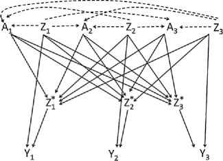
Figure 14 provides a DAG for a scenario with allocational interference and $m=3$. Within each block, we allocate the subjects into two distinct groups and each individual’s outcome may be affected by who is in each group. The DAG depicts a single block and we therefore suppress the subscript $k$. Let $Y_{i}$ be the outcome for individual $i$ and $Z_{i}$ be a vector of all baseline characteristics that affect the outcome of individual $i$ or the outcomes of the other individuals with whom he comes into contact. Define $Z_{i}^{*}$ to be an $(m-1)$-dimensional array with $j$th element equal to $Z_{j}\times I(A_{j}=A_{i})$, $j\neq i$, that is, the baseline covariates of subject $j$ multiplied by the indicator that individual $j$ is assigned to the same group as individual $i$. In addition to the individual level causal arrows from $Z_{i}$ and $Z_{i}^{*}$ into $Y_{i}$, we require arrows from $Z_{i}$ to $Z_{j}^{*}$ and from $A_{i}$ to $Z_{j}^{*}$ for all pairs $(i,j)$, $i\neq j$. This is because $Z_{j}^{*}$ is by definition a function of $\mathbf{A}$ and of $Z_{i}$ for all $i\neq j$. Randomized allocation corresponds to the absence of the dashed arrows into $\mathbf{A}$. Otherwise, an individual’s baseline covariates $Z_{i}$ may affect his group assignment $A_{i}$. For $Z_{i}$ to affect $A_{i}$ and not $A_{j}$ would entail an allocation rule that ignores balance across groups. In some settings, the vector of baseline covariates $\mathbf{Z}$ (or a function of $\mathbf{Z}$, e.g., its mean) would affect the allocation rule. This is represented by the presence of the dashed arrows into $\mathbf{A}$.

We now describe a toy example in which allocational interference operates and informs causal effects of interest. Suppose that runners enter a 5000 meter race, but the track is not wide enough for all of the competitors to race simultaneously. A race represents a single interference block; in order to perform statistical inference on the effects discussed below we would likely need to observe several independent races, indexed by $k$. The runners in each race are divided into smaller groups to race in successive heats. Number the subjects according to some composite measure of their recent performance, so that runner 1 is the fastest based on the composite measure and runner $m$ is the slowest. Let $Y_{ki}$ be the time in which runner $i$ in block $k$ finishes the race and $Z_{ki}$ be a vector of all relevant baseline characteristics. A runner’s speed will affect his own outcome. Moreover, his speed, confidence and sportsmanship may have an impact on the outcomes of the runners with whom he is grouped. These characteristics should all be included in $Z_{ki}$. The runners are divided into three heats, so $A_{ki}\in\{1,2,3\}$. For simplicity, we assume that $m$ is divisible by $3$ and each heat has $m/3$ runners, though heats of different sizes are possible. Consider the following two allocations: In allocation $\mathbf{a}$, runners 1 through $m/3$ are assigned to the first heat, runners $(m/3)+1$ through $2m/3$ to the second heat and runners $(2m/3)+1$ through $m$ to the third heat. In allocation $\mathbf{a}^{\prime}$, on the other hand, the first heat is comprised of runners $1,4,7,\ldots,m-2$; the second of runners $2,5,8,\ldots,m-1$, and the third of the remaining runners. Allocation $\mathbf{a}^{\prime}$ results in a more balanced distribution of baseline speed across heats.

Are runners, on average, likely to run faster under one of these two allocations? This is a question about the overall causal effect $E[Y(\mathbf{a})]-E[Y(\mathbf{a}^{\prime})]$. If the number of groups is the same under both allocations, as in our example, then the direct and indirect effects of allocations $\mathbf{a}$ and $\mathbf{a}^{\prime}$ may also be of interest (see Section 2.1). The expected unit-level effect $\mathit{UE}_{1}(\mathbf{a};3,1)\equiv E[Y_{1}(\mathbf{a}_{-1},3)]-E[Y_{1}(\mathbf{a}_{-1},1)]$ is the expected effect on runner 1 of racing in the fastest versus the slowest heat in allocation $\mathbf{a}$. The expected spillover effect $\mathit{SE}_{1}(\mathbf{a},\mathbf{a}^{\prime};1)\equiv E[Y_{1}(\mathbf{a}_{-1},1)]-E[Y_{1}(\mathbf{a}_{-1}^{\prime},1)]$ is the expected effect on runner 1 of running in the first heat when that heat is comprised of the fastest runners versus running in the first heat when that heat is comprised of runners with a mix of speeds. (In both cases, the expectations are with respect to multiple independent races.) This might matter if running in the first heat was advantageous because the crowd was more enthusiastic earlier on, a point to which we return below.

As always, in order to identify expectations of counterfactuals of the form $Y_{ki}(\mathbf{a}_{k})$ we require conditional exchangeability for the effect of $\mathbf{A}_{k}$ on $Y_{ki}$. If $\mathbf{A}_{k}$ and $Z_{ki}$ share any common causes, as they would if, for example, heats were assigned based on the identity of the runners’ coaches, then those common causes must be included in the conditioning set. If $A_{ki}$ depends on any component of $Z_{ki}$ then that component must be included in the conditioning set in order to achieve exchangeability. Similarly, if $A_{ki}$ depends on a component of $\mathbf{Z}_{k}$, that is, there are arrows from $Z_{ki}$ and from $Z_{kj}$, $j\neq i$, into $A_{ki}$, then that component of $\mathbf{Z}_{k}$ must be included in the conditioning set. We note that conditioning on a component of $\mathbf{Z}_{k}$ may block part of the effect of $\mathbf{A}_{k}$ on $Y_{ki}$; because $Z_{ki}^{*}$ is a deterministic function of $\mathbf{Z}_{k}$ conditioning on the latter is effectively conditioning on the former. $Z_{ki}^{*}$ lies on the causal pathway from $\mathbf{A}_{k}$ to $Y_{ki}$ and, therefore, conditioning on it blocks part of the causal effect of interest.

Figure 15:

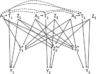
Let $T_{kl_{i}}$ be a group-level property of group $l_{i}$ in block $k$, where $l_{i}$ indexes the group to which individual $i$ is assigned, and define $T_{ki}\equiv T_{kl_{i}}$ to be the group-level property to which individual $i$ is exposed. If the order in which the heats are run makes a difference, because the weather changes throughout the day or because runners are tired later in the day, then $T_{ki}$ could be the time at which subject $i$’s heat is scheduled to race. This is an example of a preallocation group-level covariate that allows the groups to be distinguished from one another without reference to their composition. Other examples of this kind of group-level property are the teacher in charge of each classroom, the curricula to which classrooms are assigned, or different locations in which heats are assigned to run.

For the purposes of our race example, let $T_{ki}$ be a measure of the crowd enthusiasm when runner $i$ runs. The arrows from $A_{i}$ into $T_{i}$ on the DAG in Figure 15 are necessitated by the way we have defined $T_{ki}$, namely as a collection of properties of the group to which individual $i$ is assigned. Properties that depend on group composition but are not captured by $Z_{ki}^{*}$, such as the number of runners in the heat, can also affect $Y_{ki}$. Unlike the time at which each heat runs, these properties arise after group allocation and, therefore, do not distinguish the groups from one another a priori. If $T_{ki}$ is itself affected by group composition, because the size of the crowd is determined by who is in each heat, then we would also require arrows $A_{j}\rightarrow T_{i}$; these are the dashed arrows in Figure 15. Suppose that crowd enthusiasm is determined by the proportion of runners in the heat who are in the fastest quartile of all of the runners in the race, based on the baseline composite measure. Then $T_{ki}$ is affected by $\mathbf{Z}_{k}$ (which includes a measure of each runner’s previous performance), and we require arrows from each $Z_{j}$ into $T_{i}$, as on the DAG in Figure 16. If data on $\mathbf{T}_{k}$ is not collected, or if it is not known whether any group-level properties affect $Y_{ki}$, then we would add arrows from each $A_{i}$ into each $Y_{j}$ on the DAG in Figure 15, to represent the residual effect of $\mathbf{A}_{k}$ on $Y_{kj}$ due to unobserved group properties.

Figure 16:

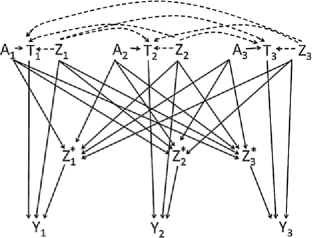
We also may be interested in whether the effect of an allocation is mediated by group attributes $\mathbf{T}_{k}$. In order to identify mediated effects through $\mathbf{T}_{k}$ it must be hypothetically possible to intervene on $\mathbf{T}_{k}$ without manipulating any other variable that may cause $Y_{ki}$ not through $\mathbf{T}_{k}$. For example, if $T_{ki}$ is the enthusiasm of the crowd when $i$’s group runs the race, then we can imagine intervening on $\mathbf{T}_{k}$ by changing the composition of the crowd without changing the assignments of runners to heats or their covariates. On the other hand, if $T_{ki}$ is the number of runners in $i$’s group, then clearly any intervention on $\mathbf{T}_{k}$ must operate because of $\mathbf{A}_{k}$, which causes $Y_{ki}$ not through $\mathbf{T}_{k}$. Natural direct, natural indirect and controlled direct effects are not coherently defined in this case. This is because counterfactuals of the form $Y_{ki}(\mathbf{a}_{k},\mathbf{T}_{k}(\mathbf{a}_{k}^{\prime}))$ are not well-defined if we cannot hypothetically simultaneously intervene on $\mathbf{A}_{k}$, setting it to $\mathbf{a}_{k}$, and on $\mathbf{T}_{k}$, setting it to its counterfactual value under allocation $\mathbf{a}_{k}^{\prime}$. If the only way to set $\mathbf{T}_{k}$ to its counterfactual value under allocation $\mathbf{a}_{k}^{\prime}$ is through an intervention that sets $\mathbf{A}_{k}$ to $\mathbf{a}_{k}^{\prime}$, then this hypothetical joint intervention is not possible. The effects of $\mathbf{A}_{k}$ on $Y_{ki}$ with $Z_{ki}^{*}$ as a mediator are similarly incoherent, because it is impossible to imagine intervening on $Z_{ki}^{*}$ without manipulating $\mathbf{A}_{k}$, $\mathbf{Z}_{k}$, or both. If we are interested in the role that $Z_{ki}^{*}$ plays in the effect of group allocation on the outcome, we can instead estimate the effects of $Z_{ki}^{*}$ on $Y_{ki}$.

5 A Note on Interference and Social Networks

Our discussion thus far has focused on settings in which individuals are clustered into blocks and in which individuals in distinct blocks do not influence each other. In some contexts, it may be the case that there are no or few distinct independent blocks; social networks constitute one such setting. A social network is a collection of individuals and the social ties between them, for example ties of friendship, kinship or physical proximity. Social networks are of public health interest because certain health-related behaviors, beliefs and outcomes may propagate socially (Christakis and Fowler, 2007, 2008; Smith and Christakis, 2008), but of course they are rife with interference, making causal inference difficult.

Allocational interference essentially involves intervening on the network structure itself, creating new ties by assigning individuals to the same group, for example, assigning children to the same classroom, and possibly breaking old ties by assigning individuals to different groups. An intervention on classroom assignments within a school could be seen as creating a new network topology at the beginning of every school year. Because the network itself is manipulated in allocational interference, it may be a useful lens through which to understand interventions on ties in social network contexts.

Contagion and direct interference occur naturally and widely in social networks. Direct interference may be present whenever an exposure consists of ideas, beliefs, knowledge or physical goods which can be shared by an exposed individual with his associates. Contagion in social networks has been written about extensively in recent years (Christakis and Fowler, 2007, 2008; Mulvaney-Day and Womack, 2009; Smith and Christakis, 2008). Infectious diseases are more likely to spread between people closely connected in a social network (e.g., because they live together or spend time together), and in addition there is some recent evidence that traits and behaviors like obesity and smoking may be “socially contagious” (Christakis and Fowler, 2007, 2008). The precise mechanisms for these purported phenomena are unknown, but some researchers have hypothesized that latent outcomes related to the observed outcomes may be transmitted through social contact. For example, Christakis and Fowler (2007, 2008) have suggested that beliefs about the acceptability of different smoking behaviors and body types may be contagious. If this is in fact the mechanism underlying what appears to be contagion of smoking behavior or obesity, then the true structure is depicted by the DAG in Figure 17. $O_{i}^{t}$ represents the observed characteristic of subject $i$ at time $t$, for example his smoking behavior, and $B_{i}^{t}$ represents his beliefs, for example, about the acceptability of smoking. We observe a phenomenon that resembles contagion, namely that $O_{i}^{t}$ appears to have a causal effect on $O_{j}^{t+1}$. However, this apparent effect may not be due to a causal pathway but rather to the backdoor path $O_{i}^{t}\leftarrow B_{i}^{t-1}\rightarrow B_{j}^{t}\rightarrow O_{j}^{t+1}$ as in Figure 17. Another possible structure that would give rise to apparent contagion is presented in Figure 18. Here, $O$ is indeed contagious, but the path by which contagion operates is mediated by $B$. Distinguishing between these different structures could have implications for interventions and policies. If the DAG in Figure 17 represents the true causal structure, then intervening on $O$ or introducing a policy targeted at affecting $O$ will not disrupt the contagious process; we should attempt to intervene on underlying beliefs instead. If the DAG in Figure 18 captures the true mechanisms at work, then intervening on either $O$ or $B$ can disrupt the contagious process.

Figure 17:

Figure 18:

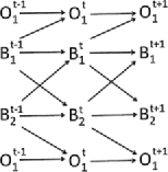
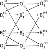
The discussion of contagion and direct interference in Section 4 may be useful for clarifying aspects of social network research. In many types of social networks and for many types of exposures and outcomes, both contagion and direct interference will be present. The results in Section 4.2.1 can sometimes be used to differentiate between the two types of interference. Contagion cannot be identified by cross-sectional network data without very strong assumptions about temporal and causal relationships, and some effects related to contagion require fine-grained information on outcomes in the network over time. Conversely, social network data can be used to refine assumptions about the structure of interference. We have assumed that interference occurred between all individuals in a block. This corresponds to a network in which each individual has a tie to every other individual in the same block. But if anything is known about the actual network topology, specifically about the absence of ties between certain individuals, then this information could be used to refine the causal structure of interference represented on the DAGs given in Section 3 and, therefore, the conditions under which causal effects are identifiable.

6 Conclusion

It is of paramount importance to carefully consider the specific causal structure whenever interference may operate on the relation between one individual’s treatment and another’s outcome. The possible structures are numerous and valid causal inference may require different assumptions in each one, depending on the effect of interest and the nature of confounding.

Also of great importance is the definition of the variables involved in the causal pathways under investigation. In some cases, the difference between interference by contagion and direct interference is contextual: depending on how we define the treatment and the outcome, some causal relationships can be seen as either one. Recall the example of direct interference that we presented in Section 4.1: the outcome is weight change and the treatment dietary counseling from a nutritionist. Direct interference occurs when a treated individual “treats” his associates by imparting to them the information gained from the nutritionist, thereby directly affecting their obesity status. Underlying this direct interference is a contagious process by which the treated individual transmits his understanding of how to adopt and maintain a healthy diet to his associates; “catching” this understanding causes the associates to lose weight. Defining variables precisely and narrowly is always a difficulty for causal inference; the challenge is to conduct valid inference when we do not observe the underlying causal mechanisms but instead have to base our analyses on constructs like weight, symptomatic flu, scholastic achievement, visits with a nutritionist, etc.

This paper scratches the surface of the enormous challenge of causal inference in the presence of interference. We have not, for example, touched upon estimation of causal effects or on inference, areas where some progress has been made in recent years (Aronow and Samii, 2013; Bowers, Fredrickson and Panagopoulos, 2013; Graham, Imbens and Ridder, 2010; Hudgens and Halloran, 2008; Manski, 2013; Rosenbaum, 2007; Tchetgen Tchetgen and VanderWeele, 2012) but much more is needed.

Appendix

We describe the identification of the effects of $A_{i}$ on $Y_{j}$ for the DAGs in Figure 5 when $\mathbf{C}$ is not fully observed.

In Figure 5(c), standardizing by $C_{i}$ identifies the effect of $A_{i}$ on $Y_{j}$:

$$\!\!\sum_{c_{i}}E[Y_{j}|A_{i}=a_{i},C_{i}=c_{i}]P(C_{i}=c)$$

$$\!\!\quad=\sum_{a_{j}}\sum_{c_{j}}\sum_{c_{i}}E[Y_{j}|A_{i}=a_{i},$$

$$\!\!\hphantom{\quad=\sum_{a_{j}}\sum_{c_{j}}\sum_{c_{i}}E[}{}C_{i}=c_{i},A_{j}=a_{j},C_{j}=c_{j}]$$

$$\!\!\hphantom{\quad=\sum_{a_{j}}\sum_{c_{j}}\sum_{c_{i}}}{}\cdot P(A_{j}=a_{j},$$

$$\!\!\hphantom{\quad=\sum_{a_{j}}\sum_{c_{j}}\sum_{c_{i}}{}\cdot P(}{}C_{j}=c_{j}|A_{i}=a_{i},C_{i}=c_{i})$$

$$\!\!\hphantom{\quad=\sum_{a_{j}}\sum_{c_{j}}\sum_{c_{i}}}{}\cdot P(C_{i}=c_{i})$$

$$\!\!\quad=\sum_{a_{j}}\sum_{c_{j}}\sum_{c_{i}}E\bigl{[}Y_{j}(a_{i},a_{j})|A_{i}=a_{i},$$

$$\!\!\hphantom{\quad=\sum_{a_{j}}\sum_{c_{j}}\sum_{c_{i}}E\bigl{[}}{}C_{i}=c_{i},A_{j}=a_{j},C_{j}=c_{j}\bigr{]}$$

$$\!\!\hphantom{\quad=\sum_{a_{j}}\sum_{c_{j}}\sum_{c_{i}}}{}\cdot P(A_{j}=a_{j},$$

$$\!\!\hphantom{\quad=\sum_{a_{j}}\sum_{c_{j}}\sum_{c_{i}}{}\cdot P(}{}C_{j}=c_{j}|A_{i}=a_{i},C_{i}=c_{i})$$

$$\!\!\hphantom{\quad=\sum_{a_{j}}\sum_{c_{j}}\sum_{c_{i}}}{}\cdot P(C_{i}=c_{i})$$

$$\quad=\sum_{a_{j}}\sum_{c_{j}}\sum_{c_{i}}E\bigl{[}Y_{j}(a_{i},a_{j})|C_{i}=c_{i},C_{j}=c_{j}\bigr{]}$$

$$\!\!\hphantom{\quad=\sum_{a_{j}}\sum_{c_{j}}\sum_{c_{i}}}{}\cdot P(A_{j}=a_{j},$$

$$\!\!\hphantom{\quad=\sum_{a_{j}}\sum_{c_{j}}\sum_{c_{i}}{}\cdot P(}{}C_{j}=c_{j}|A_{i}=a_{i},C_{i}=c_{i})$$

$$\!\!\hphantom{\quad=\sum_{a_{j}}\sum_{c_{j}}\sum_{c_{i}}}{}\cdot P(C_{i}=c_{i}).$$

This is a weighted average of $\mathbf{C}$-specific counterfactuals $Y_{j}(\mathbf{a})$. [Replacing $C_{i}$ with $D$ in the expressions above gives the identifying expression for the effect of $A_{i}$ on $Y_{j}$ in Figure 5(e).] Standardizing by $C_{i}$ also identifies the effect of $A_{i}$ on $Y_{i}$ for the DAGs in Figures 5(a) and 5(c), similarly giving a weighted average of $\mathbf{C}$-specific counterfactuals:

$$\!\!\sum_{c_{i}}E[Y_{i}|A_{i}=a_{i},C_{i}=c_{i}]P(C_{i}=c)$$

$$\!\!\quad=\sum_{a_{j}}\sum_{c_{j}}\sum_{c_{i}}E[Y_{i}|A_{i}=a_{i},$$

$$\!\!\hphantom{\quad=\sum_{a_{j}}\sum_{c_{j}}\sum_{c_{i}}E[}{}C_{i}=c_{i},A_{j}=a_{j},C_{j}=c_{j}]$$

$$\!\!\hphantom{\quad=\sum_{a_{j}}\sum_{c_{j}}\sum_{c_{i}}}{}\cdot P(A_{j}=a_{j},$$

$$\!\!\hphantom{\quad=\sum_{a_{j}}\sum_{c_{j}}\sum_{c_{i}}{}\cdot P(}{}C_{j}=c_{j}|A_{i}=a_{i},C_{i}=c_{i})$$

$$\!\!\hphantom{\quad=\sum_{a_{j}}\sum_{c_{j}}\sum_{c_{i}}}{}\cdot P(C_{i}=c_{i})$$

$$\!\!\quad=\sum_{a_{j}}\sum_{c_{j}}\sum_{c_{i}}E\bigl{[}Y_{i}(a_{i},a_{j})|A_{i}=a_{i},$$

$$\!\!\hphantom{\quad=\sum_{a_{j}}\sum_{c_{j}}\sum_{c_{i}}E\bigl{[}}{}C_{i}=c_{i},A_{j}=a_{j},C_{j}=c_{j}\bigr{]}$$

$$\!\!\hphantom{\quad=\sum_{a_{j}}\sum_{c_{j}}\sum_{c_{i}}}{}\cdot P(A_{j}=a_{j},$$

$$\!\!\hphantom{\quad=\sum_{a_{j}}\sum_{c_{j}}\sum_{c_{i}}{}\cdot P(}{}C_{j}=c_{j}|A_{i}=a_{i},C_{i}=c_{i})$$

$$\!\!\hphantom{\quad=\sum_{a_{j}}\sum_{c_{j}}\sum_{c_{i}}}{}\cdot P(C_{i}=c_{i})$$

$$\!\!\quad=\sum_{a_{j}}\sum_{c_{j}}\sum_{c_{i}}E\bigl{[}Y_{i}(a_{i},a_{j})|C_{i}=c_{i},C_{j}=c_{j}\bigr{]}$$

$$\!\!\hphantom{\quad=\sum_{a_{j}}\sum_{c_{j}}\sum_{c_{i}}}{}\cdot P(A_{j}=a_{j},$$

$$\!\!\hphantom{\quad=\sum_{a_{j}}\sum_{c_{j}}\sum_{c_{i}}{}\cdot P(}{}C_{j}=c_{j}|A_{i}=a_{i},C_{i}=c_{i})$$

$$\!\!\hphantom{\quad=\sum_{a_{j}}\sum_{c_{j}}\sum_{c_{i}}}{}\cdot P(C_{i}=c_{i}).$$

References

- Angrist and Lang (2004) {barticle}[author] \bauthor\bsnmAngrist, \bfnmJ. D.\binitsJ. D. and \bauthor\bsnmLang, \bfnmK.\binitsK. (\byear2004). \btitleDoes school integration generate peer effects? Evidence from Boston’s METCO program. \bjournalAmerican Economic Review \bvolume94 \bpages1613–1634. \bptokimsref\endbibitem
- Aronow and Samii (2013) {btechreport}[author] \bauthor\bsnmAronow, \bfnmPeter M.\binitsP. M. and \bauthor\bsnmSamii, \bfnmCyrus\binitsC. (\byear2013). \btitleEstimating average causal effects under general interference. \btypeTechnical report. \bptokimsref\endbibitem
- Avin, Shpitser and Pearl (2005) {bincollection}[author] \bauthor\bsnmAvin, \bfnmC.\binitsC., \bauthor\bsnmShpitser, \bfnmI.\binitsI. and \bauthor\bsnmPearl, \bfnmJ.\binitsJ. (\byear2005). \btitleIdentifiability of path-specific effects. In \bbooktitleProceedings of the International Joint Conference on Artificial Intelligence \bpages357–363. \bpublisherMorgan-Kaufmann, \blocationEdinburgh, UK. \bptokimsref\endbibitem
- Bowers, Fredrickson and Panagopoulos (2013) {barticle}[author] \bauthor\bsnmBowers, \bfnmJake\binitsJ., \bauthor\bsnmFredrickson, \bfnmMark M.\binitsM. M. and \bauthor\bsnmPanagopoulos, \bfnmCostas\binitsC. (\byear2013). \btitleReasoning about interference between units: A general framework. \bjournalPolitical Analysis \bvolume21 \bpages97–124. \bptokimsref\endbibitem
- Carrell, Fullerton and West (2009) {barticle}[author] \bauthor\bsnmCarrell, \bfnmS. E.\binitsS. E., \bauthor\bsnmFullerton, \bfnmR. L.\binitsR. L. and \bauthor\bsnmWest, \bfnmJ. E.\binitsJ. E. (\byear2009). \btitleDoes your cohort matter? Measuring peer effects in college achievement. \bjournalJ. Labor Economics \bvolume27 \bpages439–464. \bptokimsref\endbibitem
- Christakis and Fowler (2007) {barticle}[author] \bauthor\bsnmChristakis, \bfnmN. A.\binitsN. A. and \bauthor\bsnmFowler, \bfnmJ. H.\binitsJ. H. (\byear2007). \btitleThe spread of obesity in a large social network over 32 years. \bjournalNew England J. Medicine \bvolume357 \bpages370–379. \bptokimsref\endbibitem
- Christakis and Fowler (2008) {barticle}[author] \bauthor\bsnmChristakis, \bfnmN. A.\binitsN. A. and \bauthor\bsnmFowler, \bfnmJ. H.\binitsJ. H. (\byear2008). \btitleThe collective dynamics of smoking in a large social network. \bjournalNew England J. Medicine \bvolume358 \bpages2249–2258. \bptokimsref\endbibitem
- Cohen-Cole and Fletcher (2008) {barticle}[pbm] \bauthor\bsnmCohen-Cole, \bfnmEthan\binitsE. and \bauthor\bsnmFletcher, \bfnmJason M.\binitsJ. M. (\byear2008). \btitleIs obesity contagious? Social networks vs. environmental factors in the obesity epidemic. \bjournalJ. Health Econ. \bvolume27 \bpages1382–1387. \biddoi=10.1016/j.jhealeco.2008.04.005, issn=0167-6296, pii=S0167-6296(08)00036-2, pmid=18571258 \bptokimsref\endbibitem
- Dahlhaus and Eichler (2003) {bincollection}[mr] \bauthor\bsnmDahlhaus, \bfnmRainer\binitsR. and \bauthor\bsnmEichler, \bfnmMichael\binitsM. (\byear2003). \btitleCausality and graphical models in time series analysis. In \bbooktitleHighly Structured Stochastic Systems. \bseriesOxford Statist. Sci. Ser. \bvolume27 \bpages115–144. \bpublisherOxford Univ. Press, \blocationOxford. \bnoteWith part A by V. Didelez and part B by H. R. Künsch. \bidmr=2082408 \bptokimsref\endbibitem
- Didelez, Kreiner and Keiding (2010) {barticle}[mr] \bauthor\bsnmDidelez, \bfnmVanessa\binitsV., \bauthor\bsnmKreiner, \bfnmSvend\binitsS. and \bauthor\bsnmKeiding, \bfnmNiels\binitsN. (\byear2010). \btitleGraphical models for inference under outcome-dependent sampling. \bjournalStatist. Sci. \bvolume25 \bpages368–387. \biddoi=10.1214/10-STS340, issn=0883-4237, mr=2791673 \bptokimsref\endbibitem
- Freedman (2004) {barticle}[pbm] \bauthor\bsnmFreedman, \bfnmDavid A.\binitsD. A. (\byear2004). \btitleGraphical models for causation, and the identification problem. \bjournalEval. Rev. \bvolume28 \bpages267–293. \biddoi=10.1177/0193841X04266432, issn=0193-841X, pmid=15245621 \bptokimsref\endbibitem
- Graham, Imbens and Ridder (2010) {btechreport}[author] \bauthor\bsnmGraham, \bfnmB. S.\binitsB. S., \bauthor\bsnmImbens, \bfnmG. W.\binitsG. W. and \bauthor\bsnmRidder, \bfnmG.\binitsG. (\byear2010). \btitleMeasuring the effects of segregation in the presence of social spillovers: A nonparametric approach. \btypeTechnical report, National Bureau of Economic Research, Cambridge, MA. \bptokimsref\endbibitem
- Greenland, Pearl and Robins (1999) {barticle}[pbm] \bauthor\bsnmGreenland, \bfnmS.\binitsS., \bauthor\bsnmPearl, \bfnmJ.\binitsJ. and \bauthor\bsnmRobins, \bfnmJ. M.\binitsJ. M. (\byear1999). \btitleCausal diagrams for epidemiologic research. \bjournalEpidemiology \bvolume10 \bpages37–48. \bidissn=1044-3983, pii=00001648-199901000-00005, pmid=9888278 \bptokimsref\endbibitem
- Greenland and Robins (1986) {barticle}[pbm] \bauthor\bsnmGreenland, \bfnmS.\binitsS. and \bauthor\bsnmRobins, \bfnmJ. M.\binitsJ. M. (\byear1986). \btitleIdentifiability, exchangeability, and epidemiological confounding. \bjournalInt. J. Epidemiol. \bvolume15 \bpages413–419. \bidissn=0300-5771, pmid=3771081 \bptokimsref\endbibitem
- Halloran and Hudgens (2012) {barticle}[mr] \bauthor\bsnmHalloran, \bfnmM. Elizabeth\binitsM. E. and \bauthor\bsnmHudgens, \bfnmMichael G.\binitsM. G. (\byear2012). \btitleCausal inference for vaccine effects on infectiousness. \bjournalInt. J. Biostat. \bvolume8 \bpagesArt. 6, front matter + 40. \biddoi=10.2202/1557-4679.1354, issn=1557-4679, mr=2925328 \bptokimsref\endbibitem
- Halloran and Struchiner (1995) {barticle}[pbm] \bauthor\bsnmHalloran, \bfnmM. E.\binitsM. E. and \bauthor\bsnmStruchiner, \bfnmC. J.\binitsC. J. (\byear1995). \btitleCausal inference in infectious diseases. \bjournalEpidemiology \bvolume6 \bpages142–151. \bidissn=1044-3983, pmid=7742400 \bptokimsref\endbibitem
- Heckman, Lochner and Taber (1998) {bmisc}[author] \bauthor\bsnmHeckman, \bfnmJ. J.\binitsJ. J., \bauthor\bsnmLochner, \bfnmL.\binitsL. and \bauthor\bsnmTaber, \bfnmC.\binitsC. (\byear1998). \bhowpublishedExplaining rising wage inequality: Explorations with a dynamic general equilibrium model of labor earnings with heterogeneous agents. Technical report, National Bureau of Economic Research, Cambridge, MA. \bptokimsref\endbibitem
- Hernán and Robins (2006) {barticle}[pbm] \bauthor\bsnmHernán, \bfnmMiguel A.\binitsM. A. and \bauthor\bsnmRobins, \bfnmJames M.\binitsJ. M. (\byear2006). \btitleEstimating causal effects from epidemiological data. \bjournalJ. Epidemiol. Community Health \bvolume60 \bpages578–586. \biddoi=10.1136/jech.2004.029496, issn=0143-005X, pii=60/7/578, pmcid=2652882, pmid=16790829 \bptokimsref\endbibitem
- Hong and Raudenbush (2008) {barticle}[author] \bauthor\bsnmHong, \bfnmG.\binitsG. and \bauthor\bsnmRaudenbush, \bfnmS. W.\binitsS. W. (\byear2008). \btitleCausal inference for time-varying instructional treatments. \bjournalJ. Educational and Behavioral Statistics \bvolume33 \bpages333–362. \bptokimsref\endbibitem
- Hudgens and Halloran (2008) {barticle}[mr] \bauthor\bsnmHudgens, \bfnmMichael G.\binitsM. G. and \bauthor\bsnmHalloran, \bfnmM. Elizabeth\binitsM. E. (\byear2008). \btitleToward causal inference with interference. \bjournalJ. Amer. Statist. Assoc. \bvolume103 \bpages832–842. \biddoi=10.1198/016214508000000292, issn=0162-1459, mr=2435472 \bptokimsref\endbibitem
- Manski (2013) {barticle}[mr] \bauthor\bsnmManski, \bfnmCharles F.\binitsC. F. (\byear2013). \btitleIdentification of treatment response with social interactions. \bjournalEconom. J. \bvolume16 \bpagesS1–S23. \biddoi=10.1111/j.1368-423X.2012.00368.x, issn=1368-4221, mr=3030060 \bptokimsref\endbibitem
- Mulvaney-Day and Womack (2009) {barticle}[author] \bauthor\bsnmMulvaney-Day, \bfnmN.\binitsN. and \bauthor\bsnmWomack, \bfnmC. A.\binitsC. A. (\byear2009). \btitleObesity, identity and community: Leveraging social networks for behavior change in public health. \bjournalPublic Health Ethics \bvolume2 \bpages250–260. \bptokimsref\endbibitem
- Pearl (1995) {barticle}[mr] \bauthor\bsnmPearl, \bfnmJudea\binitsJ. (\byear1995). \btitleCausal diagrams for empirical research. \bjournalBiometrika \bvolume82 \bpages669–710. \biddoi=10.1093/biomet/82.4.669, issn=0006-3444, mr=1380809 \bptnotecheck related \bptokimsref\endbibitem
- Pearl (1997) {bincollection}[author] \bauthor\bsnmPearl, \bfnmJ.\binitsJ. (\byear1997). \btitleGraphical models for probabilistic and causal reasoning. In \bbooktitleThe Computer Science and Engineering Handbook (\beditor\bfnmA.\binitsA. \bsnmTucker, ed.) \bpages699–711. \bpublisherCRC Press, \blocationBoca Raton, FL. \bptokimsref\endbibitem
- Pearl (2000) {bbook}[mr] \bauthor\bsnmPearl, \bfnmJudea\binitsJ. (\byear2000). \btitleCausality: Models, Reasoning, and Inference. \bpublisherCambridge Univ. Press, \blocationCambridge. \bidmr=1744773 \bptokimsref\endbibitem
- Pearl (2001) {binproceedings}[author] \bauthor\bsnmPearl, \bfnmJ.\binitsJ. (\byear2001). \btitleDirect and indirect effects. In \bbooktitleProceedings of the Seventeenth Conference on Uncertainty in Artificial Intelligence \bpages411–420. \bpublisherMorgan-Kaufmann, \blocationSan Francisco, CA. \bptokimsref\endbibitem
- Pearl (2003) {barticle}[mr] \bauthor\bsnmPearl, \bfnmJudea\binitsJ. (\byear2003). \btitleStatistics and causal inference: A review. \bjournalTest \bvolume12 \bpages281–318. \biddoi=10.1007/BF02595718, issn=1133-0686, mr=2044313 \bptokimsref\endbibitem
- Pearl and Verma (1994) {bincollection}[mr] \bauthor\bsnmPearl, \bfnmJudea\binitsJ. and \bauthor\bsnmVerma, \bfnmThomas S.\binitsT. S. (\byear1994). \btitleA theory of inferred causation. In \bbooktitleLogic, Methodology and Philosophy of Science IX \bnote(Uppsala, 1991). \bseriesStud. Logic Found. Math. \bvolume134 \bpages789–811. \bpublisherNorth-Holland, \blocationAmsterdam. \biddoi=10.1016/S0049-237X(06)80074-1, mr=1328002 \bptnotecheck year \bptokimsref\endbibitem
- Richardson and Robins (2013) {bmisc}[author] \bauthor\bsnmRichardson, \bfnmThomas S.\binitsT. S. and \bauthor\bsnmRobins, \bfnmJames M.\binitsJ. M. (\byear2013). \bhowpublishedSingle World Intervention Graphs (SWIGs): A unification of the counterfactual and graphical approaches to causality. Technical Report 128, Center for Statistics and the Social Sciences, Univ. Washington, Seattle, WA. \bptokimsref\endbibitem
- Robins (2003) {bincollection}[mr] \bauthor\bsnmRobins, \bfnmJ. M.\binitsJ. M. (\byear2003). \btitleSemantics of causal DAG models and the identification of direct and indirect effects. In \bbooktitleHighly Structured Stochastic Systems (\beditor\bfnmP. J.\binitsP. J. \bsnmGreen, \beditor\bfnmN. L.\binitsN. L. \bsnmHjort and \beditor\bfnmS.\binitsS. \bsnmRichardson, eds.) \bpages70–82. \bseriesOxford Statistical Science Series \bvolume27. \bpublisherOxford Univ. Press, \blocationOxford. \bidmr=2082403 \bptokimsref\endbibitem
- Rosenbaum (2007) {barticle}[mr] \bauthor\bsnmRosenbaum, \bfnmPaul R.\binitsP. R. (\byear2007). \btitleInterference between units in randomized experiments. \bjournalJ. Amer. Statist. Assoc. \bvolume102 \bpages191–200. \biddoi=10.1198/016214506000001112, issn=0162-1459, mr=2345537 \bptokimsref\endbibitem
- Ross (1916) {barticle}[author] \bauthor\bsnmRoss, \bfnmR.\binitsR. (\byear1916). \btitleAn application of the theory of probabilities to the study of a priori pathometry. Part I. \bjournalProc. R. Soc. Lond. Ser. A Math. Phys. Eng. Sci. \bvolume92 \bpages204. \bptokimsref\endbibitem
- Rubin (1990) {barticle}[mr] \bauthor\bsnmRubin, \bfnmDonald B.\binitsD. B. (\byear1990). \btitleComment on J. Neyman and causal inference in experiments and observational studies: “On the application of probability theory to agricultural experiments. Essay on principles. Section 9” [Ann. Agric. Sci. 10 (1923) 1–51]. \bjournalStatist. Sci. \bvolume5 \bpages472–480. \bidissn=0883-4237, mr=1092987 \bptnotecheck related \bptokimsref\endbibitem
- Sacerdote (2000) {bmisc}[author] \bauthor\bsnmSacerdote, \bfnmB.\binitsB. (\byear2000). \bhowpublishedPeer effects with random assignment: Results for Dartmouth roommates. Technical report, National Bureau of Economic Research, Cambridge, MA. \bptokimsref\endbibitem
- Smith and Christakis (2008) {barticle}[author] \bauthor\bsnmSmith, \bfnmK. P.\binitsK. P. and \bauthor\bsnmChristakis, \bfnmN. A.\binitsN. A. (\byear2008). \btitleSocial networks and health. \bjournalAnnual Revue of Sociology \bvolume34 \bpages405–429. \bptokimsref\endbibitem
- Sobel (2006) {barticle}[mr] \bauthor\bsnmSobel, \bfnmMichael E.\binitsM. E. (\byear2006). \btitleWhat do randomized studies of housing mobility demonstrate?: Causal inference in the face of interference. \bjournalJ. Amer. Statist. Assoc. \bvolume101 \bpages1398–1407. \biddoi=10.1198/016214506000000636, issn=0162-1459, mr=2307573 \bptokimsref\endbibitem
- Tchetgen Tchetgen and VanderWeele (2012) {barticle}[mr] \bauthor\bsnmTchetgen Tchetgen, \bfnmEric J.\binitsE. J. and \bauthor\bsnmVanderWeele, \bfnmTyler J.\binitsT. J. (\byear2012). \btitleOn causal inference in the presence of interference. \bjournalStat. Methods Med. Res. \bvolume21 \bpages55–75. \biddoi=10.1177/0962280210386779, issn=0962-2802, mr=2867538 \bptokimsref\endbibitem
- Tian and Pearl (2002a) {bincollection}[author] \bauthor\bsnmTian, \bfnmJ.\binitsJ. and \bauthor\bsnmPearl, \bfnmJ.\binitsJ. (\byear2002a). \btitleA general identification condition for causal effects. In \bbooktitleProceedings of the National Conference on Artificial Intelligence \bpages567–573. \bpublisherMIT Press, \blocationCambridge, MA. \bptokimsref\endbibitem
- Tian and Pearl (2002b) {binproceedings}[author] \bauthor\bsnmTian, \bfnmJin\binitsJ. and \bauthor\bsnmPearl, \bfnmJudea\binitsJ. (\byear2002b). \btitleOn the testable implications of causal models with hidden variables. In \bbooktitleProceedings of the Eighteenth Conference on Uncertainty in Artificial Intelligence \bpages519–527. \bpublisherMorgan Kaufmann, \blocationSan Francisco, CA. \bptokimsref\endbibitem
- VanderWeele (2010) {barticle}[mr] \bauthor\bsnmVanderWeele, \bfnmTyler J.\binitsT. J. (\byear2010). \btitleDirect and indirect effects for neighborhood-based clustered and longitudinal data. \bjournalSociol. Methods Res. \bvolume38 \bpages515–544. \biddoi=10.1177/0049124110366236, issn=0049-1241, mr=2758165 \bptokimsref\endbibitem
- VanderWeele and Hernan (2013) {barticle}[author] \bauthor\bsnmVanderWeele, \bfnmT. J.\binitsT. J. and \bauthor\bsnmHernan, \bfnmM. A.\binitsM. A. (\byear2013). \btitleCausal inference under multiple versions of treatment. \bjournalJ. Causal Inference \bvolume1 \bpages1–20. \bptokimsref\endbibitem
- VanderWeele and Tchetgen Tchetgen (2011a) {barticle}[pbm] \bauthor\bsnmVanderWeele, \bfnmTyler J.\binitsT. J. and \bauthor\bsnmTchetgen Tchetgen, \bfnmEric J.\binitsE. J. (\byear2011a). \btitleBounding the infectiousness effect in vaccine trials. \bjournalEpidemiology \bvolume22 \bpages686–693. \biddoi=10.1097/EDE.0b013e31822708d5, issn=1531-5487, mid=NIHMS496622, pmcid=3792580, pmid=21753730 \bptokimsref\endbibitem
- VanderWeele and Tchetgen Tchetgen (2011b) {barticle}[mr] \bauthor\bsnmVanderWeele, \bfnmTyler J.\binitsT. J. and \bauthor\bsnmTchetgen Tchetgen, \bfnmEric J.\binitsE. J. (\byear2011b). \btitleEffect partitioning under interference in two-stage randomized vaccine trials. \bjournalStatist. Probab. Lett. \bvolume81 \bpages861–869. \biddoi=10.1016/j.spl.2011.02.019, issn=0167-7152, mr=2793754 \bptokimsref\endbibitem
- Vanderweele, Tchetgen and Halloran (2012) {barticle}[pbm] \bauthor\bsnmVanderWeele, \bfnmTyler J.\binitsT. J., \bauthor\bsnmTchetgen Tchetgen, \bfnmEric J.\binitsE. J. and \bauthor\bsnmHalloran, \bfnmM. Elizabeth\binitsM. E. (\byear2012). \btitleComponents of the indirect effect in vaccine trials: Identification of contagion and infectiousness effects. \bjournalEpidemiology \bvolume23 \bpages751–761. \biddoi=10.1097/EDE.0b013e31825fb7a0, issn=1531-5487, mid=NIHMS386535, pmcid=3415570, pmid=22828661 \bptokimsref\endbibitem
- VanderWeele et al. (2013) {barticle}[mr] \bauthor\bsnmVanderWeele, \bfnmTyler J.\binitsT. J., \bauthor\bsnmHong, \bfnmGuanglei\binitsG., \bauthor\bsnmJones, \bfnmStephanie M.\binitsS. M. and \bauthor\bsnmBrown, \bfnmJoshua L.\binitsJ. L. (\byear2013). \btitleMediation and spillover effects in group-randomized trials: A case study of the 4Rs educational intervention. \bjournalJ. Amer. Statist. Assoc. \bvolume108 \bpages469–482. \biddoi=10.1080/01621459.2013.779832, issn=0162-1459, mr=3174634 \bptokimsref\endbibitem
- Vansteelandt (2007) {barticle}[mr] \bauthor\bsnmVansteelandt, \bfnmStijn\binitsS. (\byear2007). \btitleOn confounding, prediction and efficiency in the analysis of longitudinal and cross-sectional clustered data. \bjournalScand. J. Stat. \bvolume34 \bpages478–498. \biddoi=10.1111/j.1467-9469.2006.00555.x, issn=0303-6898, mr=2368794 \bptokimsref\endbibitem
- Verma (1993) {bmisc}[author] \bauthor\bsnmVerma, \bfnmT. S.\binitsT. S. (\byear1993). \bhowpublishedGraphical aspects of causal models. Technical Report R-191, Univ. California, Los Angeles, CA. \bptokimsref\endbibitem