thanks: Author to whom correspondence should be sent.

Topological implications of negative curvature for biological and social networks

Réka Albert ralbert@phys.psu.edu www.phys.psu.edu/~ralbert Department of Physics, Pennsylvania State University, University Park, PA 16802    Bhaskar DasGupta dasgupta@cs.uic.edu www.cs.uic.edu/~dasgupta Department of Computer Science, University of Illinois at Chicago, Chicago, IL 60607    Nasim Mobasheri nmobas2@uic.edu Department of Computer Science, University of Illinois at Chicago, Chicago, IL 60607
Abstract

Network measures that reflect the most salient properties of complex large-scale networks are in high demand in the network research community. In this paper we adapt a combinatorial measure of negative curvature (also called hyperbolicity) to parameterized finite networks, and show that a variety of biological and social networks are hyperbolic. This hyperbolicity property has strong implications on the higher-order connectivity and other topological properties of these networks. Specifically, we derive and prove bounds on the distance among shortest or approximately shortest paths in hyperbolic networks. We describe two implications of these bounds to cross-talk in biological networks, and to the existence of central, influential neighborhoods in both biological and social networks.

Hyperbolicity, Networks, Crosstalk, Influential nodes
pacs:
87.18.Mp,87.18.Cf,87.18.Vf,89.75.Hc,02.10.Ox

I Introduction

For a large variety of complex systems, ranging from the World-Wide Web to metabolic networks, representation as a parameterized network and graph theoretical analysis of this network have led to many useful insights Newman-book ; AB-review . In addition to established network measures such as the average degree, clustering coefficient or diameter, complex network researchers have proposed and evaluated a number novel network measures rich-club ; LM07 ; albert-et-al-2011 ; bassett-et-al-2011 . In this article we consider a combinatorial measure of negative curvature (also called hyperbolicity) of parameterized finite networks and the implications of negative curvature on the higher-order connectivity and topological properties of these networks.

There are many ways in which the (positive or negative) curvature of a continuous surface or other similar spaces can be defined depending on whether the measure is to reflect the local or global properties of the underlying space. The specific notion of negative curvature that we use is an adoption of the hyperbolicity measure for a infinite metric space with bounded local geometry as originally proposed by Gromov G87 using a so-called “444-point condition”. We adopt this measure for parameterized finite discrete metric spaces induced by a network via all-pairs shortest paths and apply it to biological and social networks. Recently, there has been a surge of empirical works measuring and analyzing the hyperbolicity of networks defined in this manner, and many real-world networks were observed to be hyperbolic in this sense. For example, preferential attachment networks were shown to be scaled hyperbolic in JL04 ; JLB07 , networks of high power transceivers in a wireless sensor network were empirically observed to have a tendency to be hyperbolic in ALJKZ08 , communication networks at the IP layer and at other levels were empirically observed to be hyperbolic in NS11 ; PKBV10 , extreme congestion at a very limited number of nodes in a very large traffic network was shown in JLBB11 to be caused due to hyperbolicity of the network together with minimum length routing, and the authors in BPK10 showed how to efficiently map the topology of the Internet to a hyperbolic space.

Gromov’s hyperbolicity measure adopted on a shortest-path metric of networks can also be visualized as a measure of the “closeness” of the original network topology to a tree topology MSV11 . Another popular measure used in both the bioinformatics and theoretical computer science literature is the treewidth measure first introduced by Robertson and Seymour RS83 . Many 𝖭𝖯𝖭𝖯\mathsf{NP}-hard problems on general networks admit efficient polynomial-time solutions if restricted to classes of networks with bounded treewidth B88 , just as several routing-related problems or the diameter estimation problem become easier if the network has small hyperbolicity CE07 ; CDEHV08 ; CDEHVX12 ; GL05 . However, as observed in MSV11 , the two measures are quite different in nature: “the treewidth is more related to the least number of nodes whose removal changes the connectivity of the graph in a significant manner whereas the hyperbolicity measure is related to comparing the geodesics of the given network with that of a tree”. Other related research works on hyperbolic networks include estimating the distortion necessary to map hyperbolic metrics to tree metrics ABKMRT07 and studying the algorithmic aspects of several combinatorial problems on points in a hyperbolic space KL06 .

II Hyperbolicity-related Definitions and Measures

Let G=(V,E)𝐺𝑉𝐸G=(V,E) be a connected undirected graph of n4𝑛4n\geq 4 nodes. We will use the following notations:

  • u𝒫vsuperscript𝒫𝑢𝑣u\!\stackrel{{\scriptstyle\mathcal{P}}}{{\leftrightsquigarrow}}\!v denotes a path 𝒫(u=u0,u1,,uk1,uk=v)𝒫formulae-sequence𝑢subscript𝑢0subscript𝑢1subscript𝑢𝑘1subscript𝑢𝑘𝑣\mathcal{P}\equiv\left(u=u_{0},u_{1},\dots,u_{k-1},u_{k}=v\right) from node u𝑢u to node v𝑣v and (𝒫)𝒫\ell(\mathcal{P}) denotes the length (number of edges) of such a path.

  • ui𝒫ujsuperscript𝒫subscript𝑢𝑖subscript𝑢𝑗u_{i}\!\stackrel{{\scriptstyle\mathcal{P}}}{{\leftrightsquigarrow}}\!u_{j} denotes the sub-path (ui,ui+1,,uj)subscript𝑢𝑖subscript𝑢𝑖1subscript𝑢𝑗\left(u_{i},u_{i+1},\dots,u_{j}\right) of 𝒫𝒫\mathcal{P} from uisubscript𝑢𝑖u_{i} to ujsubscript𝑢𝑗u_{j}.

  • u𝔰vsuperscript𝔰𝑢𝑣u\!\stackrel{{\scriptstyle\mathfrak{s}}}{{\leftrightsquigarrow}}\!v denotes a shortest path from node u𝑢u to node v𝑣v of length du,v=(u𝔰v)subscript𝑑𝑢𝑣superscript𝔰𝑢𝑣d_{u,v}=\ell\big{(}u\!\stackrel{{\scriptstyle\mathfrak{s}}}{{\leftrightsquigarrow}}\!v\big{)}.

We introduce the hyperbolicity measures via the 444-node condition as originally proposed by Gromov. Consider a quadruple of distinct nodes111If two or more nodes among u1,u2,u3,u4subscript𝑢1subscript𝑢2subscript𝑢3subscript𝑢4u_{1},u_{2},u_{3},u_{4} are identical, then δu1,u2,u3,u4+=0subscriptsuperscript𝛿subscript𝑢1subscript𝑢2subscript𝑢3subscript𝑢40\delta^{+}_{u_{1},u_{2},u_{3},u_{4}}=0 due to the metric’s triangle inequality; thus it suffices to assume that the four nodes are distinct. u1,u2,u3,u4subscript𝑢1subscript𝑢2subscript𝑢3subscript𝑢4u_{1},u_{2},u_{3},u_{4}, and let π=(π1,π2,π3,π4)𝜋subscript𝜋1subscript𝜋2subscript𝜋3subscript𝜋4\pi=\left(\pi_{1},\pi_{2},\pi_{3},\pi_{4}\right) be a permutation of {1,2,3,4}1234\{1,2,3,4\} denoting a rearrangement of the indices of nodes such that

Su1,u2,u3,u4=duπ1,uπ2+duπ3,uπ4Mu1,u2,u3,u4=duπ1,uπ3+duπ2,uπ4Lu1,u2,u3,u4=duπ1,uπ4+duπ2,uπ3subscript𝑆subscript𝑢1subscript𝑢2subscript𝑢3subscript𝑢4subscript𝑑subscript𝑢subscript𝜋1subscript𝑢subscript𝜋2subscript𝑑subscript𝑢subscript𝜋3subscript𝑢subscript𝜋4subscript𝑀subscript𝑢1subscript𝑢2subscript𝑢3subscript𝑢4subscript𝑑subscript𝑢subscript𝜋1subscript𝑢subscript𝜋3subscript𝑑subscript𝑢subscript𝜋2subscript𝑢subscript𝜋4subscript𝐿subscript𝑢1subscript𝑢2subscript𝑢3subscript𝑢4subscript𝑑subscript𝑢subscript𝜋1subscript𝑢subscript𝜋4subscript𝑑subscript𝑢subscript𝜋2subscript𝑢subscript𝜋3S_{u_{1},u_{2},u_{3},u_{4}}=d_{u_{\pi_{1}},u_{\pi_{2}}}+d_{u_{\pi_{3}},u_{\pi_{4}}}\\ \leq M_{u_{1},u_{2},u_{3},u_{4}}=d_{u_{\pi_{1}},u_{\pi_{3}}}+d_{u_{\pi_{2}},u_{\pi_{4}}}\\ \leq L_{u_{1},u_{2},u_{3},u_{4}}=d_{u_{\pi_{1}},u_{\pi_{4}}}+d_{u_{\pi_{2}},u_{\pi_{3}}}

and let δu1,u2,u3,u4+=Lu1,u2,u3,u4Mu1,u2,u3,u42subscriptsuperscript𝛿subscript𝑢1subscript𝑢2subscript𝑢3subscript𝑢4subscript𝐿subscript𝑢1subscript𝑢2subscript𝑢3subscript𝑢4subscript𝑀subscript𝑢1subscript𝑢2subscript𝑢3subscript𝑢42\delta^{+}_{u_{1},u_{2},u_{3},u_{4}}=\frac{L_{u_{1},u_{2},u_{3},u_{4}}-M_{u_{1},u_{2},u_{3},u_{4}}}{2}. Considering all combinations of four nodes in a graph one can define a worst-case hyperbolicityG87 as

δworst+(G)=maxu1,u2,u3,u4{δu1,u2,u3,u4+}subscriptsuperscript𝛿worst𝐺subscriptsubscript𝑢1subscript𝑢2subscript𝑢3subscript𝑢4subscriptsuperscript𝛿subscript𝑢1subscript𝑢2subscript𝑢3subscript𝑢4\delta^{+}_{\mathrm{worst}}(G)=\max_{u_{1},u_{2},u_{3},u_{4}}\left\{\,\delta^{+}_{u_{1},u_{2},u_{3},u_{4}}\right\}

and an average hyperbolicity as

δave+(G)=1(n4)u1,u2,u3,u4δu1,u2,u3,u4+subscriptsuperscript𝛿ave𝐺1binomial𝑛4subscriptsubscript𝑢1subscript𝑢2subscript𝑢3subscript𝑢4subscriptsuperscript𝛿subscript𝑢1subscript𝑢2subscript𝑢3subscript𝑢4\delta^{+}_{\mathrm{ave}}(G)=\frac{1}{\binom{n}{4}}\sum_{\hskip 14.45377ptu_{1},u_{2},u_{3},u_{4}}\delta^{+}_{u_{1},u_{2},u_{3},u_{4}}

Note that δave+(G)subscriptsuperscript𝛿ave𝐺\delta^{+}_{\mathrm{ave}}(G) is the expected value of δu1,u2,u3,u4+subscriptsuperscript𝛿subscript𝑢1subscript𝑢2subscript𝑢3subscript𝑢4\delta^{+}_{u_{1},u_{2},u_{3},u_{4}} when the four nodes u1,u2,u3,u4subscript𝑢1subscript𝑢2subscript𝑢3subscript𝑢4u_{1},u_{2},u_{3},u_{4} are picked independently and uniformly at random from the set of all nodes. Both δworst+(G)subscriptsuperscript𝛿worst𝐺\delta^{+}_{\mathrm{worst}}(G) and δave+(G)subscriptsuperscript𝛿ave𝐺\delta^{+}_{\mathrm{ave}}(G) can be trivially computed in O(n4)superscript𝑛4\big{(}n^{4}\big{)} time for any graph G𝐺G.

A graph G𝐺G is called δ𝛿\delta-hyperbolic if δworst+(G)δsubscriptsuperscript𝛿worst𝐺𝛿\delta^{+}_{\mathrm{worst}}(G)\leq\delta. If δ𝛿\delta is a small constant independent of the parameters of the graph, a δ𝛿\delta-hyperbolic graph is simply called a hyperbolic graph. It is easy to see that if G𝐺G is a tree then δworst+(G)=δave+(G)=0subscriptsuperscript𝛿worst𝐺subscriptsuperscript𝛿ave𝐺0\delta^{+}_{\mathrm{worst}}(G)=\delta^{+}_{\mathrm{ave}}(G)=0. Thus all trees are hyperbolic graphs.

The hyperbolicity measure δworst+subscriptsuperscript𝛿worst\delta^{+}_{\mathrm{worst}} considered in this paper for a metric space was originally used by Gromov in the context of group theory G87 by observing that many results concerning the fundamental group of a Riemann surface hold true in a more general context. δworst+subscriptsuperscript𝛿worst\delta^{+}_{\mathrm{worst}} is trivially infinite in the standard (unbounded) Euclidean space. Intuitively, a metric space has a finite value of δworst+subscriptsuperscript𝛿worst\delta^{+}_{\mathrm{worst}} if it behaves metrically in the large scale as a negatively curved Riemannian manifold, and thus the value of δworst+subscriptsuperscript𝛿worst\delta^{+}_{\mathrm{worst}} can be related to the standard scalar curvature of a Hyperbolic manifold. For example, a simply connected complete Riemannian manifold whose sectional curvature is below α<0𝛼0\alpha<0 has a value of δworst+subscriptsuperscript𝛿worst\delta^{+}_{\mathrm{worst}} that is O((α)1)Osuperscript𝛼1\mathrm{O}\left({\left(\sqrt{-\alpha}\,\right)}^{-1}\right) (see R96 ).

In this paper we first show that a variety of biological and social networks are hyperbolic. We formulate and prove bounds on the existence of path-chords and on the distance among shortest or approximately shortest paths in hyperbolic networks. We determine the implications of these bounds on regulatory networks, i.e., directed networks whose edges correspond to regulation or influence. This category includes all the biological networks that we study in this paper. We also discuss the implications of our results on the region of influence of nodes in social networks. Some of the proofs of our theoretical results are adaptation of corresponding arguments in the continuous hyperbolic space. All the proofs are presented in the appendix for the sake of completeness.

Table 1: Hyperbolicity and diameter values for biological networks.

[0.8] Network id reference Average degree δave+(G)subscriptsuperscript𝛿ave𝐺\delta^{+}_{\mathrm{ave}}(G) δworst+(G)subscriptsuperscript𝛿worst𝐺\delta^{+}_{\mathrm{worst}}(G) 𝒟𝒟\mathcal{D} δworst+(G)𝒟/2subscriptsuperscript𝛿worst𝐺𝒟2\dfrac{\delta^{+}_{\mathrm{worst}}(G)}{\nicefrac{{\mathcal{D}}}{{2}}} 1. E. coli transcriptional net1 1.451.451.45 0.1320.1320.132 222 101010 0.4000.4000.400 2. Mammalian Signaling net2 2.042.042.04 0.0130.0130.013 333 111111 0.5450.5450.545 3. E. Coli transcriptional bold-♯\boldsymbol{\sharp} 1.301.301.30 0.0430.0430.043 222 131313 0.3080.3080.308 4. T LGL signaling net6 2.322.322.32 0.2970.2970.297 222 777 0.5710.5710.571 5. S. cerevisiae transcriptional net8 1.561.561.56 0.0040.0040.004 333 151515 0.4000.4000.400 6. C. elegans Metabolic net10-1 4.504.504.50 0.0100.0100.010 1.51.51.5 777 0.4290.4290.429 7. Drosophila segment polarity Odell:2000 1.691.691.69 0.6760.6760.676 444 999 0.8890.8890.889 8. ABA signaling LAA06 1.601.601.60 0.3020.3020.302 222 777 0.5710.5710.571 9. Immune Response Network Thakar07 2.332.332.33 0.2860.2860.286 1.51.51.5 444 0.7500.7500.750 10. T Cell Receptor Signalling julio07 1.461.461.46 0.3230.3230.323 333 131313 0.4620.4620.462 11. Oriented yeast PPI net11 3.113.113.11 0.0010.0010.001 222 666 0.6670.6670.667 bold-♯{}^{\textstyle\boldsymbol{\sharp}}\,(net1, , updated version)     see www.weizmann.ac.il/mcb/UriAlon/Papers/networkMotifs/coli1_1Inter_st.txt

Table 2: Hyperbolicity and diameter values for social networks.

[0.8] Network id reference Average degree δave+(G)subscriptsuperscript𝛿ave𝐺\delta^{+}_{\mathrm{ave}}(G) δworst+(G)subscriptsuperscript𝛿worst𝐺\delta^{+}_{\mathrm{worst}}(G) 𝒟𝒟\mathcal{D} δworst+(G)𝒟/2subscriptsuperscript𝛿worst𝐺𝒟2\dfrac{\delta^{+}_{\mathrm{worst}}(G)}{\nicefrac{{\mathcal{D}}}{{2}}} 1. Dolphins social network LSBHSD03 5.165.165.16 0.2620.2620.262 222 888 0.7500.7500.750 2. American College Football GN02 10.6410.6410.64 0.3120.3120.312 222 555 0.8000.8000.800 3. Zachary Karate Club Z77 4.584.584.58 0.1700.1700.170 111 555 0.4000.4000.400 4. Books about US Politics bold-‡\boldsymbol{\ddagger} 8.418.418.41 0.2470.2470.247 222 777 0.5710.5710.571 5. Sawmill communication MM97 3.443.443.44 0.1620.1620.162 111 888 0.2500.2500.250 6. Jazz musician GD03 27.6927.6927.69 0.1400.1400.140 1.51.51.5 666 0.5000.5000.500 7. Visiting ties in San Juan LMCL53 3.843.843.84 0.4220.4220.422 333 999 0.6670.6670.667 8. World Soccer data, 199819981998 bold-†\boldsymbol{\dagger} 3.373.373.37 0.2700.2700.270 2.52.52.5 121212 0.2860.2860.286 9. Les Miserable Knu93 6.516.516.51 0.2780.2780.278 222 141414 0.4170.4170.417 bold-‡\,{}^{\textstyle\boldsymbol{\ddagger}}\,V. Krebs, www.orgnet.com, bold-†{}^{\textstyle\boldsymbol{\dagger}}\,Dagstuhl seminar: Link Analysis and Visualization, Dagstuhl 1-6, 2001;     vlado.fmf.uni-lj.si/pub/networks/data/sport/football.htm

III Results and Discussion

Subsection A examines in detail the hyperbolicity of an assorted list of diverse biological and social networks. The remaining subsections of this section, namely subsections B–E, state our findings on the implications of hyperbolicity of a network on various topological properties of the network. For subsections D, E, we first state our findings as applicable for biological or social networks, followed by a summary of formal mathematical results that led to such findings. Because the precise bounds on topological features of a network as a function of hyperbolicty measures are quite mathematically involved, we discuss these bounds in a somewhat simplified form in subsections B–E, leaving the precise bounds as theorems and proofs in the appendix.

III.1 Hyperbolicity of Real Networks

We analyzed twenty well-known biological and social networks. The 111111 biological networks shown in Table 2 include 333 transcriptional regulatory, 555 signalling, 111 metabolic, 111 immune response and 111 oriented protein-protein interaction networks. Similarly, the 999 social networks shown in Table 2 range from interactions in dolphin communities to the social network of jazz musicians. The hyperbolicity of the biological and directed social networks was computed by ignoring the direction of edges. The hyperbolicity values were calculated by writing codes in C using standard algorithmic procedures.

As shown on Table 2 and Table 2, the hyperbolicity values of almost all networks are small. If 𝒟=maxu,v{du,v}𝒟subscript𝑢𝑣subscript𝑑𝑢𝑣\mathcal{D}=\max_{u,v}\big{\{}d_{u,v}\big{\}} is the diameter of the graph, then it is easy to see that δworst+(G)𝒟/2subscriptsuperscript𝛿worst𝐺𝒟2\delta^{+}_{\mathrm{worst}}(G)\leq\nicefrac{{\mathcal{D}}}{{2}}, and thus small diameter indeed implies a small value of worst-case hyperbolicity. As can be seen on Table 2 and Table 2, δworst+(G)subscriptsuperscript𝛿worst𝐺\delta^{+}_{\mathrm{worst}}(G) varies with respect to its worst-case bound of 𝒟/2𝒟2\nicefrac{{\mathcal{D}}}{{2}} from 25%percent2525\% of 𝒟/2𝒟2\nicefrac{{\mathcal{D}}}{{2}} to no more than 89%percent8989\% of 𝒟/2𝒟2\nicefrac{{\mathcal{D}}}{{2}}, and there does not seem to be a systematic dependence of δworst+(G)subscriptsuperscript𝛿worst𝐺\delta^{+}_{\mathrm{worst}}(G) on the number of nodes (which ranges from 181818 to 786786786), edges (from 424242 to 274227422742), or on the value of the diameter 𝒟𝒟\mathcal{D}.

For all the networks δave+(G)subscriptsuperscript𝛿ave𝐺\delta^{+}_{\mathrm{ave}}(G) is one or two orders of magnitude smaller than δworst+(G)subscriptsuperscript𝛿worst𝐺\delta^{+}_{\mathrm{worst}}(G). Intuitively, this suggests that the value of δworst+(G)subscriptsuperscript𝛿worst𝐺\delta^{+}_{\mathrm{worst}}(G) may be a rare deviation from typical values of δu1,u2,u3,u4+subscriptsuperscript𝛿subscript𝑢1subscript𝑢2subscript𝑢3subscript𝑢4\delta^{+}_{u_{1},u_{2},u_{3},u_{4}} that one would obtain for most combinations of nodes {u1,u2,u3,u4}subscript𝑢1subscript𝑢2subscript𝑢3subscript𝑢4\left\{u_{1},u_{2},u_{3},u_{4}\right\}.

We additionally performed the following rigorous tests for hyperbolicity of our networks.

III.1.1 Checking hyperbolicity via the scaled hyperbolicity approach

An approach for testing hyperbolicity for finite graphs was introduced and used via “scaled” Gromov hyperbolicity in JLB07 ; NS11 for hyperbolicity defined via thin triangles and in JLA11 for for hyperbolicity defined via the four-point condition as used in this paper. The basic idea is to “scale” the values of δu1,u2,u3,u4+subscriptsuperscript𝛿subscript𝑢1subscript𝑢2subscript𝑢3subscript𝑢4\delta^{+}_{u_{1},u_{2},u_{3},u_{4}} by a suitable scaling factor, say μu1,u2,u3,u4subscript𝜇subscript𝑢1subscript𝑢2subscript𝑢3subscript𝑢4\mu_{u_{1},u_{2},u_{3},u_{4}}, such that there exists a constant 0<ε<10𝜀10<\varepsilon<1 with the following property:

  • the maximum achievable value of δu1,u2,u3,u4+μu1,u2,u3,u4subscriptsuperscript𝛿subscript𝑢1subscript𝑢2subscript𝑢3subscript𝑢4subscript𝜇subscript𝑢1subscript𝑢2subscript𝑢3subscript𝑢4\frac{\delta^{+}_{u_{1},u_{2},u_{3},u_{4}}}{\mu_{u_{1},u_{2},u_{3},u_{4}}} is ε𝜀\varepsilon in the standard hyperbolic space or in the Euclidean space, and

  • δu1,u2,u3,u4+μu1,u2,u3,u4subscriptsuperscript𝛿subscript𝑢1subscript𝑢2subscript𝑢3subscript𝑢4subscript𝜇subscript𝑢1subscript𝑢2subscript𝑢3subscript𝑢4\frac{\delta^{+}_{u_{1},u_{2},u_{3},u_{4}}}{\mu_{u_{1},u_{2},u_{3},u_{4}}} goes beyond ε𝜀\varepsilon in positively curved spaces.

We use the notation 𝒟u1,u2,u3,u4=maxi,j{1,2,3,4}{dui,uj}subscript𝒟subscript𝑢1subscript𝑢2subscript𝑢3subscript𝑢4subscript𝑖𝑗1234subscript𝑑subscript𝑢𝑖subscript𝑢𝑗\displaystyle\mathcal{D}_{u_{1},u_{2},u_{3},u_{4}}=\max_{i,j\in\{1,2,3,4\}}\left\{d_{u_{i},u_{j}}\right\} to indicate the diameter of the subset of four nodes u1,u2,u3subscript𝑢1subscript𝑢2subscript𝑢3u_{1},u_{2},u_{3} and u4subscript𝑢4u_{4}. By using theoretical or empirical calculations, the authors in JLA11 provide the bounds shown in Table 3.

Table 3:  JLA11 Various scaled Gromov hyperbolicities.

[0.9] Name Notation μu1,u2,u3,u4subscript𝜇subscript𝑢1subscript𝑢2subscript𝑢3subscript𝑢4\mu_{u_{1},u_{2},u_{3},u_{4}} ε𝜀\varepsilon Method for determining ε𝜀\varepsilon diameter-scaled hyperbolicity δ𝒟superscript𝛿𝒟\delta^{\mathrm{\mathcal{D}}} 𝒟u1,u2,u3,u4subscript𝒟subscript𝑢1subscript𝑢2subscript𝑢3subscript𝑢4\mathcal{D}_{u_{1},u_{2},u_{3},u_{4}} 0.29290.29290.2929     empirical L𝐿L-scaled hyperbolicity δLsuperscript𝛿L\delta^{\mathrm{L}} Lu1,u2,u3,u4subscript𝐿subscript𝑢1subscript𝑢2subscript𝑢3subscript𝑢4L_{u_{1},u_{2},u_{3},u_{4}} 21222122\!\!\!\!\!\!\frac{\sqrt{2}-1}{2\sqrt{2}} \approx 0.14640.1464\!\!0.1464    mathematical (L+M+S)𝐿𝑀𝑆(L+M+S)-scaled hyperbolicity δL+M+Ssuperscript𝛿LMS\delta^{\mathrm{L+M+S}} Lu1,u2,u3,u4subscript𝐿subscript𝑢1subscript𝑢2subscript𝑢3subscript𝑢4L_{u_{1},u_{2},u_{3},u_{4}} +Mu1,u2,u3,u4subscript𝑀subscript𝑢1subscript𝑢2subscript𝑢3subscript𝑢4\,\,+\,M_{u_{1},u_{2},u_{3},u_{4}} +Su1,u2,u3,u4subscript𝑆subscript𝑢1subscript𝑢2subscript𝑢3subscript𝑢4\,\,\,\,\,\,+\,S_{u_{1},u_{2},u_{3},u_{4}} 0.06070.06070.0607    mathematical

Table 4: ΔY(G)superscriptΔY𝐺\Delta^{\mathrm{Y}}(G) values for biological networks for Y{𝒟,L,L+M+S}𝑌𝒟𝐿𝐿𝑀𝑆Y\in\left\{\mathcal{D},\,L,\,L+M+S\right\}.

[1] Network id Δ𝒟(G)superscriptΔ𝒟𝐺\Delta^{\mathrm{\mathcal{D}}}(G) ΔL(G)superscriptΔL𝐺\Delta^{\mathrm{L}}(G) ΔL+M+S(G)superscriptΔLMS𝐺\Delta^{\mathrm{L+M+S}}(G) 1. E. coli transcriptional 0.00140.00140.0014 0.00180.00180.0018 0.00150.00150.0015 2. Mammalian Signaling 0.00210.00210.0021 0.00180.00180.0018 0.00220.00220.0022 3. E. Coli transcriptional 0.00060.00060.0006 0.00060.00060.0006 0.00070.00070.0007 4. T LGL signaling 0.02280.02280.0228 0.02210.02210.0221 0.03180.03180.0318 5. S. cerevisiae transcriptional 0.00310.00310.0031 0.00320.00320.0032 0.00330.00330.0033 6. C. elegans Metabolic 0.00200.00200.0020 0.00180.00180.0018 0.00190.00190.0019 7. Drosophila segment polarity 0.03740.03740.0374 0.05580.0558\mathbf{0.0558} 0.07500.07500.0750 8. ABA signaling 0.03430.03430.0343 0.02850.02850.0285 0.04250.04250.0425 9. Immune Response Network 0.04610.0461\mathbf{0.0461} 0.05520.05520.0552 0.07810.0781\mathbf{0.0781} 10. T Cell Receptor Signalling 0.00340.00340.0034 0.00450.00450.0045 0.00560.00560.0056 11. Oriented yeast PPI 0.00130.00130.0013 0.00090.00090.0009 0.00120.00120.0012 maximum 0.04610.04610.0461 0.05580.05580.0558 0.07810.07810.0781

Table 5: ΔY(G)superscriptΔY𝐺\Delta^{\mathrm{Y}}(G) values for social networks for Y{𝒟,L,L+M+S}𝑌𝒟𝐿𝐿𝑀𝑆Y\in\left\{\mathcal{D},\,L,\,L+M+S\right\}.

[1] Network id Δ𝒟(G)superscriptΔ𝒟𝐺\Delta^{\mathrm{\mathcal{D}}}(G) ΔL(G)superscriptΔL𝐺\Delta^{\mathrm{L}}(G) ΔL+M+S(G)superscriptΔLMS𝐺\Delta^{\mathrm{L+M+S}}(G) 1. Dolphins social network 0.01150.01150.0115 0.01200.01200.0120 0.01680.01680.0168 2. American College Football 0.04350.0435\mathbf{0.0435} 0.03950.0395\mathbf{0.0395} 0.05770.0577\mathbf{0.0577} 3. Zachary Karate Club 0.01950.01950.0195 0.02490.02490.0249 0.02840.02840.0284 4. Books about US Politics 0.01060.01060.0106 0.00740.00740.0074 0.01160.01160.0116 5. Sawmill communication 0.00690.00690.0069 0.00680.00680.0068 0.00850.00850.0085 6. Jazz musician 0.00970.00970.0097 0.01170.01170.0117 0.01240.01240.0124 7. Visiting ties in San Juan 0.02210.02210.0221 0.02420.02420.0242 0.02750.02750.0275 8. World Soccer data, 199819981998 0.01450.01450.0145 0.01550.01550.0155 0.02120.02120.0212 9. Les Miserable 0.00320.00320.0032 0.00340.00340.0034 0.00490.00490.0049 maximum 0.04350.04350.0435 0.03950.03950.0395 0.05770.05770.0577

We adapt the criterion proposed by Jonckheere, Lohsoonthorn and Ariaei JLA11 to designate a given finite graph as hyperbolic by requiring a significant percentage of all possible subset of four nodes to satisfy the ε𝜀\varepsilon bound. More formally, suppose that G𝐺G has t𝑡t connected components containing n1,n2,,ntsubscript𝑛1subscript𝑛2subscript𝑛𝑡n_{1},n_{2},\dots,n_{t} nodes, respectively (j=1tnj=nsuperscriptsubscript𝑗1𝑡subscript𝑛𝑗𝑛\sum_{j=1}^{t}n_{j}=n). Let 0<η<10𝜂10<\eta<1 be a sufficiently high value indicating the confidence level in declaring the graph G𝐺G to be hyperbolic. Then, we call our given graph G𝐺G to be (scaled) hyperbolic if and only if

ΔY(G)= 
number of subset of four nodes {ui,uj,uk,u}
such that >δYui,uj,uk,uε
 
 
number of all possible combinations of four nodes
that contribute to hyperbolicity
 
= 
number of subset of four nodes {ui,uj,uk,u}
such that >δYui,uj,uk,uε
 
1jt:nj>3(nj4)
<1η
superscriptΔY𝐺 
number of subset of four nodes {ui,uj,uk,u}
such that >δYui,uj,uk,uε
 
 
number of all possible combinations of four nodes
that contribute to hyperbolicity
 
 
number of subset of four nodes {ui,uj,uk,u}
such that >δYui,uj,uk,uε
 
subscript:1𝑗𝑡subscript𝑛𝑗3binomialsubscript𝑛𝑗4
1𝜂
\Delta^{\mathrm{Y}}(G)=\frac{\text{ \begin{tabular}[]{c}\small number of subset of four nodes $\left\{u_{i},u_{j},u_{k},u_{\ell}\right\}$\\ \small such that $\delta^{\mathrm{Y}}_{u_{i},u_{j},u_{k},u_{\ell}}>\varepsilon$\end{tabular} }}{\text{ \begin{tabular}[]{c}\small number of all possible combinations of four nodes\\ \small that contribute to hyperbolicity\end{tabular} }}\\ =\frac{\text{ \begin{tabular}[]{c}\small number of subset of four nodes $\left\{u_{i},u_{j},u_{k},u_{\ell}\right\}$\\ \small such that $\delta^{\mathrm{Y}}_{u_{i},u_{j},u_{k},u_{\ell}}>\varepsilon$\end{tabular} }}{\sum_{1\leq j\leq t\colon n_{j}>3}\binom{n_{j}}{4}}<1-\eta

The values of ΔY(G)superscriptΔY𝐺\Delta^{\mathrm{Y}}(G) for our networks are shown in Table 5 and Table 5. It can be seen that, for all scaled hyperbolicity measures and for all networks, the value of 1η1𝜂1-\eta is very close to zero.

Table 6: p𝑝p-values for the ΔY(G)superscriptΔY𝐺\Delta^{\mathrm{Y}}(G) values for biological networks for Y{𝒟,L,L+M+S}𝑌𝒟𝐿𝐿𝑀𝑆Y\in\left\{\mathcal{D},\,L,\,L+M+S\right\}. In general, a p𝑝p-value less than 0.050.050.05 (shown in boldface) is considered to be statistically significant, and a p𝑝p-value above 0.050.050.05 is considered to be not statistically significant.

[0.87] Network id 1. E. coli 2. Mammalian Signaling 3. E. Coli transcriptional 4. T LGL signaling 5. S. cerevisiae transcriptional 6. C. elegans Metabolic 7. Drosophila segment polarity 8. ABA signaling 9. Immune Response Network 10. T Cell Receptor Signalling 11. Oriented yeast PPI p𝑝p values Δ𝒟superscriptΔ𝒟\Delta^{\mathrm{\mathcal{D}}} 0.00180.0018\mathbf{0.0018} <0.0001absent0.0001\mathbf{<0.0001} <0.0001absent0.0001\mathbf{<0.0001} <0.0001absent0.0001\mathbf{<0.0001} 0.33210.33210.3321 <0.0001absent0.0001\mathbf{<0.0001} <0.0001absent0.0001\mathbf{<0.0001} <0.0001absent0.0001\mathbf{<0.0001} <0.0001absent0.0001\mathbf{<0.0001} <0.0001absent0.0001\mathbf{<0.0001} <0.0001absent0.0001\mathbf{<0.0001} ΔLsuperscriptΔL\Delta^{\mathrm{L}} <0.0001absent0.0001\mathbf{<0.0001} <0.0001absent0.0001\mathbf{<0.0001} <0.0001absent0.0001\mathbf{<0.0001} 0.0110.0110.011 0.34340.34340.3434 <0.0001absent0.0001\mathbf{<0.0001} <0.0001absent0.0001\mathbf{<0.0001} 0.91450.91450.9145 <0.0001absent0.0001\mathbf{<0.0001} <0.0001absent0.0001\mathbf{<0.0001} <0.0001absent0.0001\mathbf{<0.0001} ΔL+M+SsuperscriptΔLMS\Delta^{\mathrm{L+M+S}} 0.52260.52260.5226 <0.0001absent0.0001\mathbf{<0.0001} <0.0001absent0.0001\mathbf{<0.0001} <0.0001absent0.0001\mathbf{<0.0001} 0.34240.34240.3424 <0.0001absent0.0001\mathbf{<0.0001} <0.0001absent0.0001\mathbf{<0.0001} 0.33420.33420.3342 <0.0001absent0.0001\mathbf{<0.0001} <0.0001absent0.0001\mathbf{<0.0001} <0.0001absent0.0001\mathbf{<0.0001}

Table 7: p𝑝p-values for the ΔY(G)superscriptΔY𝐺\Delta^{\mathrm{Y}}(G) values for social networks for Y{𝒟,L,L+M+S}𝑌𝒟𝐿𝐿𝑀𝑆Y\in\left\{\mathcal{D},\,L,\,L+M+S\right\}. In general, a p𝑝p-value less than 0.050.050.05 (shown in boldface) is considered to be statistically significant, and a p𝑝p-value above 0.050.050.05 is considered to be not statistically significant.

[1] Network id 1. Dolphins social network 2. American College Football 3. Zachary Karate Club 4. Books about US Politics 5. Sawmill communication 6. Jazz musician 7. Visiting ties in San Juan 8. World Soccer data, 199819981998 9. Les Miserable p𝑝p values Δ𝒟superscriptΔ𝒟\Delta^{\mathrm{\mathcal{D}}} <0.0001absent0.0001\mathbf{<0.0001} <0.0001absent0.0001\mathbf{<0.0001} <0.0001absent0.0001\mathbf{<0.0001} <0.0001absent0.0001\mathbf{<0.0001} <0.0001absent0.0001\mathbf{<0.0001} <0.0001absent0.0001\mathbf{<0.0001} <0.0001absent0.0001\mathbf{<0.0001} <0.0001absent0.0001\mathbf{<0.0001} <0.0001absent0.0001\mathbf{<0.0001} ΔLsuperscriptΔL\Delta^{\mathrm{L}} <0.0001absent0.0001\mathbf{<0.0001} <0.0001absent0.0001\mathbf{<0.0001} <0.0001absent0.0001\mathbf{<0.0001} <0.0001absent0.0001\mathbf{<0.0001} <0.0001absent0.0001\mathbf{<0.0001} <0.0001absent0.0001\mathbf{<0.0001} 0.07790.07790.0779 <0.0001absent0.0001\mathbf{<0.0001} <0.0001absent0.0001\mathbf{<0.0001} ΔL+M+SsuperscriptΔLMS\Delta^{\mathrm{L+M+S}} <0.0001absent0.0001\mathbf{<0.0001} <0.0001absent0.0001\mathbf{<0.0001} <0.0001absent0.0001\mathbf{<0.0001} <0.0001absent0.0001\mathbf{<0.0001} <0.0001absent0.0001\mathbf{<0.0001} <0.0001absent0.0001\mathbf{<0.0001} <0.0001absent0.0001\mathbf{<0.0001} <0.0001absent0.0001\mathbf{<0.0001} <0.0001absent0.0001\mathbf{<0.0001}

We next tested the statistical significance of the ΔY(G)superscriptΔY𝐺\Delta^{\mathrm{Y}}(G) values by computing the statistical significance values (commonly called p𝑝p-values) of these ΔY(G)superscriptΔY𝐺\Delta^{\mathrm{Y}}(G) values for each network G𝐺G with respect to a null hypothesis model of the networks. We use a standard method used in the network science literature (e.g., see albert-et-al-2011 ; net1 ) for such purpose. For each network G𝐺G, we generated 100100100 randomized versions of the network using a Markov-chain algorithm KTV99 by swapping the endpoints of randomly selected pairs of edges until 20%percent2020\% of the edges was changed. We computed the values of ΔY(Grand1)superscriptΔYsubscript𝐺subscriptrand1\Delta^{\mathrm{Y}}\left(G_{\mathrm{rand}_{1}}\right), ΔY(Grand2)superscriptΔYsubscript𝐺subscriptrand2\Delta^{\mathrm{Y}}\left(G_{\mathrm{rand}_{2}}\right), \dots, ΔY(Grand100)superscriptΔYsubscript𝐺subscriptrand100\Delta^{\mathrm{Y}}\left(G_{\mathrm{rand}_{100}}\right). We then used an (unpaired) one-sample student’s t-test to determine the probability that ΔY(G)superscriptΔY𝐺\Delta^{\mathrm{Y}}(G) belongs to the same distribution as ΔY(Grand1)superscriptΔYsubscript𝐺subscriptrand1\Delta^{\mathrm{Y}}\left(G_{\mathrm{rand}_{1}}\right), ΔY(Grand2)superscriptΔYsubscript𝐺subscriptrand2\Delta^{\mathrm{Y}}\left(G_{\mathrm{rand}_{2}}\right), \dots, ΔY(Grand100)superscriptΔYsubscript𝐺subscriptrand100\Delta^{\mathrm{Y}}\left(G_{\mathrm{rand}_{100}}\right).

The p𝑝p-values, tabulated in Table 6 and Table 7, clearly show that all social networks and all except two biological networks can be classified as hyperbolic in a statistically significant manner, implying that the topologies of these networks are close to a “tree topology”. Indeed, for biological networks, the assumption of chain-like or tree-like topology is frequently made in the traditional molecular biology literature Alberts-1994 . Independent current observations also provide evidence of tree-like topologies for various biological networks, e.g., the average in/out degree of transcriptional regulatory networks net1 ; Lee-et-al-2002 and of a mammalian signal transduction network net2 is close to 111, so cycles are very rare.

Refer to caption
Figure 1: Path-chord of a cycle 𝒞=(u0.u1,u2,u3,u4,u5,u0)\mathcal{C}=\left(u_{0}.u_{1},u_{2},u_{3},u_{4},u_{5},u_{0}\right).

III.2 Hyperbolicity and crosstalk in regulatory networks

Let 𝒞=(u0,u1,,uk1,u0)𝒞subscript𝑢0subscript𝑢1subscript𝑢𝑘1subscript𝑢0\mathcal{C}=\left(u_{0},u_{1},\dots,u_{k-1},u_{0}\right) be a cycle of k4𝑘4k\geq 4 nodes. A path-chord of 𝒞𝒞\mathcal{C} is defined to be a path ui𝒫ujsuperscript𝒫subscript𝑢𝑖subscript𝑢𝑗u_{i}\!\stackrel{{\scriptstyle\mathcal{P}}}{{\leftrightsquigarrow}}\!u_{j} between two distinct nodes ui,uj𝒞subscript𝑢𝑖subscript𝑢𝑗𝒞u_{i},u_{j}\in\mathcal{C} such that the length of 𝒫𝒫\mathcal{P} is less than (ij)(modk)annotated𝑖𝑗pmod𝑘(i-j)\pmod{k} (see Fig. 1). A path-chord of length 111 is simply called a chord.

We find that large cycles without a path-chord imply large lower bounds on hyperbolicity (see Theorem 1 in Section A of the appendix). In particular, G𝐺G does not have a cycle of more than 4δworst+(G)4subscriptsuperscript𝛿worst𝐺4\,\delta^{+}_{\mathrm{worst}}(G) nodes that does not have a path-chord. Thus, for example, if δworst+(G)<1subscriptsuperscript𝛿worst𝐺1\delta^{+}_{\mathrm{worst}}(G)<1 then G𝐺G has no chordless cycle, i.e., G𝐺G is a chordal graph. The intuition behind the proof of Theorem 1 is that if G𝐺G contains a long cycle without a path-chord then we can select four almost equidistant nodes on the cycle and these nodes give a large hyperbolicity value. This general result has the following implications for regulatory networks:

  • If a node regulates itself through a long feedback loop (e.g., of length at least 666 if δworst+(G)=3/2subscriptsuperscript𝛿worst𝐺32\delta^{+}_{\mathrm{worst}}(G)=\nicefrac{{3}}{{2}}) then this loop must have a path-chord. Thus it follows that there exists a shorter feedback cycle through the same node.

  • A chord or short path-chord can be interpreted as crosstalk between two paths between a pair of nodes. With this interpretation, the following conclusion follows. If one node in a regulatory network regulates another node through two sufficiently long paths, then there must be a crosstalk path between these two paths. For example, assuming δworst+(G)=3/2subscriptsuperscript𝛿worst𝐺32\delta^{+}_{\mathrm{worst}}(G)=\nicefrac{{3}}{{2}}, there must be a crosstalk path if the sum of lengths of the two paths is at least 666. In general, the number of crosstalk paths between two paths increases at least linearly with the total length of the two paths. The general conclusion that can be drawn is that independent linear pathways that connect a signal to the same output node (e.g., transcription factor) are rare, and if multiple pathways exist then they are interconnected through cross-talks.

III.3 Shortest-path triangles and crosstalk paths in regulatory networks

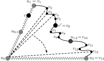
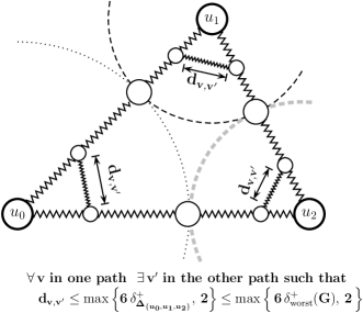
(a) Result related to triplets of shortest paths Originally, the hyperbolicity measure was introduced for infinite continuous metric spaces with negative curvature via the concept of the “thin” and “slim” triangles (e.g., see book ). For finite discrete metric spaces as induced by an undirected graph, one can analogously define a shortest-path triangle (or, simply a triangle) Δ{u0,u1,u2}subscriptΔsubscript𝑢0subscript𝑢1subscript𝑢2\Delta_{\left\{u_{0},u_{1},u_{2}\right\}} as a set of three distinct nodes u0,u1,u2subscript𝑢0subscript𝑢1subscript𝑢2u_{0},u_{1},u_{2} with a set of three shortest paths 𝒫Δ(u0,u1)subscript𝒫Δsubscript𝑢0subscript𝑢1\mathcal{P}_{\Delta}\left(u_{0},u_{1}\right), 𝒫Δ(u0,u2)subscript𝒫Δsubscript𝑢0subscript𝑢2\mathcal{P}_{\Delta}\left(u_{0},u_{2}\right), 𝒫Δ(u1,u2)subscript𝒫Δsubscript𝑢1subscript𝑢2\mathcal{P}_{\Delta}\left(u_{1},u_{2}\right) between u0subscript𝑢0u_{0} and u1subscript𝑢1u_{1}, u0subscript𝑢0u_{0} and u2subscript𝑢2u_{2}, and u1subscript𝑢1u_{1} and u2subscript𝑢2u_{2}, respectively. As illustrated on Fig. 2, in hyperbolic networks we are guaranteed to find short paths222By a short path here, we mean a path whose length is at most a constant times δΔ{u0,u1,u2}+subscriptsuperscript𝛿subscriptΔsubscript𝑢0subscript𝑢1subscript𝑢2\delta^{+}_{\Delta_{\{u_{0},u_{1},u_{2}\}}} (note that δΔ{u0,u1,u2}+δworst+(G)subscriptsuperscript𝛿subscriptΔsubscript𝑢0subscript𝑢1subscript𝑢2subscriptsuperscript𝛿worst𝐺\delta^{+}_{\Delta_{\{u_{0},u_{1},u_{2}\}}}\leq\delta^{+}_{\mathrm{worst}}(G)). between the nodes that make up 𝒫Δ(u0,u1)subscript𝒫Δsubscript𝑢0subscript𝑢1\mathcal{P}_{\Delta}\left(u_{0},u_{1}\right), 𝒫Δ(u0,u2)subscript𝒫Δsubscript𝑢0subscript𝑢2\mathcal{P}_{\Delta}\left(u_{0},u_{2}\right), 𝒫Δ(u1,u2)subscript𝒫Δsubscript𝑢1subscript𝑢2\mathcal{P}_{\Delta}\left(u_{1},u_{2}\right). This is formally stated in Theorem 3 in Section B of the appendix. Moreover, as Corollary 4 (in Section B of the appendix) states, we can have a small Hausdorff distance between these shortest paths. This result is a proper generalization of our previous result on path-cords. Indeed, in the special case when u1subscript𝑢1u_{1} and u2subscript𝑢2u_{2} are the same node the triangle becomes a shortest-path cycle involving the shortest paths between u0subscript𝑢0u_{0} and u1subscript𝑢1u_{1} and the short-cord result is obtained.

A proof of Theorem 3 is obtained by appropriate modification of a known similar bound for infinite continuous metric spaces.

The implications of this result for regulatory networks can be summarized as follows:

If we consider a feedback loop (cycle) or feed-forward loop formed by the shortest paths among three nodes, we can expect short cross-talk paths between these shortest paths. Consequently, the feedback or feed-forward loop will be nested with “additional” feed-back or feed-forward loops in which one of the paths will be slightly longer.

The above finding is empirically supported by the observation that network motifs (e.g., feed-forward or feed-back loops composed of three nodes and three edges) are often nested albert-review .
Refer to caption
Figure 2: An informal and simplified pictorial illustration of the claims in Section III.3(a).
Refer to caption
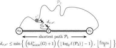
Figure 3: An informal and simplified pictorial illustration of the claims in Section III.3(b).

(b) Results related to the distance between two exact or approximate shortest paths between the same pair of nodes It is reasonable to assume that, when up- or down-regulation of a target node is mediated by two or more short paths 333Here by short paths we mean either a shortest path or an approximately shortest path whose length is not too much above the length of a shortest path, i.e., a μ𝜇\mu-approximate short path or a ε𝜀\varepsilon-additive-approximate short path, as defined in the subsequent “Formal Justifications and Intuitions” subsection, for small μ𝜇\mu or small ε𝜀\varepsilon, respectively. starting from the same regulator node, additional very long paths between the same regulator and target node do not contribute significantly to the target node’s regulation. We refer to the short paths as relevant, and to the long paths as irrelevant. Then, our finding can be summarized by saying that:

almost all relevant paths between two nodes have crosstalk paths between each other.

Formal Justifications and Intuitions (see Theorem 5 and Corollary 6 in Section C and Theorem 7 and Corollary 8 in Section D of the appendix)

We use the following two quantifications of “approximately” short paths:

  • A path u0𝒫uk=(u0,u1,,uk)superscript𝒫subscript𝑢0subscript𝑢𝑘subscript𝑢0subscript𝑢1subscript𝑢𝑘u_{0}\!\stackrel{{\scriptstyle\mathcal{P}}}{{\leftrightsquigarrow}}\!u_{k}=\big{(}u_{0},u_{1},\dots,u_{k}\big{)} is μ𝜇\mu-approximate short provided (ui𝒫uj)μdui,ujsuperscript𝒫subscript𝑢𝑖subscript𝑢𝑗𝜇subscript𝑑subscript𝑢𝑖subscript𝑢𝑗\ell\big{(}u_{i}\!\stackrel{{\scriptstyle\mathcal{P}}}{{\leftrightsquigarrow}}\!u_{j}\big{)}\leq\mu\,d_{u_{i},u_{j}} for all 0i<jk0𝑖𝑗𝑘0\leq i<j\leq k,

  • A path u0𝒫uksuperscript𝒫subscript𝑢0subscript𝑢𝑘u_{0}\!\stackrel{{\scriptstyle\mathcal{P}}}{{\leftrightsquigarrow}}\!u_{k} is ε𝜀\varepsilon-additive-approximate short provided (𝒫)du0,uk+ε𝒫subscript𝑑subscript𝑢0subscript𝑢𝑘𝜀\ell\left(\mathcal{P}\right)\leq d_{u_{0},u_{k}}+\varepsilon.

A mathematical justification for the claim then is provided by two separate theorems and their corollaries:

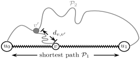
  • Let 𝒫1subscript𝒫1\mathcal{P}_{1} and 𝒫2subscript𝒫2\mathcal{P}_{2} be a shortest path and an arbitrary path, respectively, between two nodes u0subscript𝑢0u_{0} and u1subscript𝑢1u_{1}. Then, Theorem 5 and Corollary 6 implies that, for every node v𝑣v on 𝒫1subscript𝒫1\mathcal{P}_{1}, there exists a node vsuperscript𝑣v^{\prime} on 𝒫2subscript𝒫2\mathcal{P}_{2} such that dv,vsubscript𝑑𝑣superscript𝑣d_{v,v^{\prime}} depends linearly on δworst+(G)subscriptsuperscript𝛿worst𝐺\delta^{+}_{\mathrm{worst}}(G), only logarithmically on the length of 𝒫2subscript𝒫2\mathcal{P}_{2} and does not depend on the size or any other parameter of the network.

    To obtain this type of bound, one needs to apply Theorem 3 on u0subscript𝑢0u_{0}, u1subscript𝑢1u_{1} and the middle node of the path 𝒫2subscript𝒫2\mathcal{P}_{2} and then use the same approach recursively on a part of the path 𝒫2subscript𝒫2\mathcal{P}_{2} containing at most (𝒫2)/2subscript𝒫22\left\lceil\nicefrac{{\left(\mathcal{P}_{2}\right)}}{{2}}\right\rceil edges. The depth of the level of recursion provides the logarithmic factor in the bound.

  • If 𝒫1subscript𝒫1\mathcal{P}_{1} and 𝒫2subscript𝒫2\mathcal{P}_{2} are two short paths between u0subscript𝑢0u_{0} and u1subscript𝑢1u_{1} then Theorem 7 and Corollary 8 imply that the Hausdorff distance between 𝒫1subscript𝒫1\mathcal{P}_{1} and 𝒫2subscript𝒫2\mathcal{P}_{2} depends on δworst+(G)subscriptsuperscript𝛿worst𝐺\delta^{+}_{\mathrm{worst}}(G) only and does not depend on the size or any other parameter of the network.

    Intuitively, Theorem 7 and Corollary 8 can be thought of as generalizing and improving the bound in Theorem 5 for approximately short paths.

Refer to caption
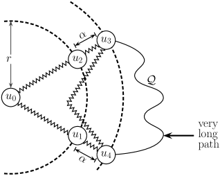
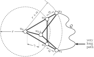
Figure 4: An informal and simplified pictorial illustration of claim ()(\star) in Section III.4. As the nodes u3subscript𝑢3u_{3} and u4subscript𝑢4u_{4} move further away from the center node u0subscript𝑢0u_{0}, the shortest path between them bends more towards u0subscript𝑢0u_{0} and any path between them that does not involve a node in the ball rrBr(u0)subscriptsuperscript𝑟𝑟subscript𝐵superscript𝑟subscript𝑢0\cup_{r^{\prime}\leq r}B_{r^{\prime}}\left(u_{0}\right) is long enough.

III.4 Identifying essential edges in the regulation between two nodes

For a given ξ>0𝜉0\xi>0 and a node u𝑢u, let ξ(u)={v|du,v=ξ}subscript𝜉𝑢conditional-set𝑣subscript𝑑𝑢𝑣𝜉\mathcal{B}_{\xi}\,(u)=\left\{\,v\,|\,d_{u,v}=\xi\,\right\} denote the “boundary of the ξ𝜉\xi-neighborhood” of u𝑢u, i.e., the set of all nodes at a distance of precisely ξ𝜉\xi from u𝑢u. Our two findings in the present context are as stated in (I) and (II) below.

(I) Identifying relevant paths between a source and a target node Suppose that we pick a node v𝑣v and consider the strict ξ𝜉\xi-neighborhood of v𝑣v

Nξ+(v)=rξr(v){u|degree of u is one}subscriptsuperscript𝑁𝜉𝑣subscript𝑟𝜉subscriptsuperscript𝑟𝑣conditional-set𝑢degree of u is one\displaystyle N^{+}_{\xi}(v)=\bigcup_{r\leq\xi}\mathcal{B}_{r^{\prime}}\left(v\right)\setminus\big{\{}u\,|\,\text{degree of $u$ is one}\big{\}}

(i.e., the set of all nodes, excluding nodes of degree 111, that are at a distance at most ξ𝜉\xi from u𝑢u) for a sufficiently large ξ𝜉\xi. Consider two nodes u1subscript𝑢1u_{1} and u2subscript𝑢2u_{2} on the boundary of this neighborhood, i.e., at a distance ξ𝜉\xi from v𝑣v. Then, the following holds:

(\star) the relevant (short) regulatory paths between u1subscript𝑢1u_{1} and u2subscript𝑢2u_{2} do not leave the neighborhood, i.e., all the edges in the relevant regulatory paths are in the neighborhood.

Thus, only the edges inside the neighborhood are relevant to the regulation among this pair of nodes.

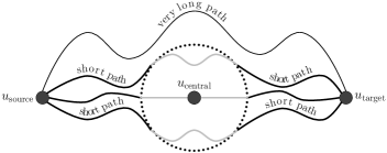
This result can be adapted to find the most relevant paths between the input node usourcesubscript𝑢sourceu_{\mathrm{source}} and output node utargetsubscript𝑢targetu_{\mathrm{target}} of a signal transduction network. In many situations, for example when the signal transduction network is inferred from undirected protein-protein interaction data, a large number of paths can potentially be included in the signal transduction network as the protein-protein interaction network has a large connected component with a small average path length albert-review . There is usually no prior knowledge on which of the existing paths are relevant to the signal transduction network. A hyperbolicity-based method is to first find a central node ucentralsubscript𝑢centralu_{\mathrm{central}} which is at equal distance between usourcesubscript𝑢sourceu_{\mathrm{source}} and utargetsubscript𝑢targetu_{\mathrm{target}}, and is on the shortest, or close to shortest, path between usourcesubscript𝑢sourceu_{\mathrm{source}} and utargetsubscript𝑢targetu_{\mathrm{target}}. Then one constructs the neighborhood around ucentralsubscript𝑢centralu_{\mathrm{central}} such that usourcesubscript𝑢sourceu_{\mathrm{source}} and utargetsubscript𝑢targetu_{\mathrm{target}} are on the boundary of this neighborhood. Applying this result, the paths relevant to the signal transduction network are inside the neighborhood, and the paths that go out of the neighborhood are irrelevant. See Fig. 4 for a pictorial illustration of this implication.
Refer to caption
Figure 5: An informal and simplified pictorial illustration of claim ()(\star\!\star) in Section III.4. Knocking out the nodes in a small neighborhood of ucentralsubscript𝑢centralu_{\mathrm{central}} cuts off all relevant (short) regulation between usourcesubscript𝑢sourceu_{\mathrm{source}} and utargetsubscript𝑢targetu_{\mathrm{target}}.

(II) Finding essential nodes Again, consider an input node usourcesubscript𝑢sourceu_{\mathrm{source}} and output node utargetsubscript𝑢targetu_{\mathrm{target}} of a signal transduction network, and let ucentralsubscript𝑢centralu_{\mathrm{central}} be a central node which is on the shortest path between them and at approximately equal distance between usourcesubscript𝑢sourceu_{\mathrm{source}} and utargetsubscript𝑢targetu_{\mathrm{target}}. Our results show that444O and ΩΩ\Omega are the standard notations used in analyzing asymptotic upper and lower bounds in the computer science literature: given two functions f(n)𝑓𝑛f(n) and g(n)𝑔𝑛g(n) of a variable n𝑛n, f(n)=O(g(n))𝑓𝑛O𝑔𝑛f(n)=\mathrm{O}(g(n)) (respectively, f(n)=Ω(g(n))𝑓𝑛Ω𝑔𝑛f(n)=\Omega(g(n)) provided there exists two constants n0,c>0subscript𝑛0𝑐0n_{0},c>0 such that f(n)cg(n)𝑓𝑛𝑐𝑔𝑛f(n)\leq c\,g(n) (respectively, f(n)cg(n)𝑓𝑛𝑐𝑔𝑛f(n)\geq c\,g(n)) for nn0𝑛subscript𝑛0n\geq n_{0}.

(\star\!\star) if one constructs a small ξ𝜉\xi-neighbourhood around ucentralsubscript𝑢centralu_{\mathrm{central}} with ξ=O(δworst+(G))𝜉Osubscriptsuperscript𝛿worst𝐺\xi=\text{O}\left(\delta^{+}_{\mathrm{worst}}(G)\right), then all relevant (short or approximately short) paths between usourcesubscript𝑢sourceu_{\mathrm{source}} and utargetsubscript𝑢targetu_{\mathrm{target}} must include a node in this ξ𝜉\xi-neighborhood. Therefore, “knocking out” the nodes in this ξ𝜉\xi-neighborhood cuts off all relevant regulatory paths between usourcesubscript𝑢sourceu_{\mathrm{source}} and utargetsubscript𝑢targetu_{\mathrm{target}}.

See Fig. 5 for a pictorial illustration of this implication. Note that the size ξ𝜉\xi of the neighborhood depends only on δworst+(G)subscriptsuperscript𝛿worst𝐺\delta^{+}_{\mathrm{worst}}(G) which, as our empirical results indicate, is usually a small constant for real networks.

Formal Justifications and Intuitions for ()(\star) and ()(\star\!\star) (see Theorem 10 and Corollary 11 in Section E of the appendix)

Suppose that we are given the following:

  • three integers κ4𝜅4\kappa\geq 4, α>0𝛼0\alpha>0,
    r>(κ21)(6δworst+(G)+2)𝑟𝜅216subscriptsuperscript𝛿worst𝐺2r>\left(\frac{\kappa}{2}-1\right)\left(6\,\delta^{+}_{\mathrm{worst}}(G)+2\right),

  • five nodes u0,u1,u2,u3,u4subscript𝑢0subscript𝑢1subscript𝑢2subscript𝑢3subscript𝑢4u_{0},u_{1},u_{2},u_{3},u_{4} such that

    • u1,u2Br(u0)subscript𝑢1subscript𝑢2subscript𝐵𝑟subscript𝑢0u_{1},u_{2}\in B_{r}\left(u_{0}\right) with du1,u2κ2(6δworst+(G)+2)subscript𝑑subscript𝑢1subscript𝑢2𝜅26subscriptsuperscript𝛿worst𝐺2d_{u_{1},u_{2}}\geq\frac{\kappa}{2}\,\left(6\,\delta^{+}_{\mathrm{worst}}(G)+2\right),

    • du1,u4=du2,u3=αsubscript𝑑subscript𝑢1subscript𝑢4subscript𝑑subscript𝑢2subscript𝑢3𝛼d_{u_{1},u_{4}}=d_{u_{2},u_{3}}=\alpha.

Then, ()(\star) and ()(\star\!\star) are implied by following type of asymptotic bounds provided by Theorem 10 and Corollary 11:

For a suitable positive value λ=O(δworst+(G))𝜆Osubscriptsuperscript𝛿worst𝐺\lambda=\mathrm{O}\big{(}\delta^{+}_{\mathrm{worst}}(G)\,\big{)}, if du1,u4=du2,u3=α>λsubscript𝑑subscript𝑢1subscript𝑢4subscript𝑑subscript𝑢2subscript𝑢3𝛼𝜆d_{u_{1},u_{4}}=d_{u_{2},u_{3}}=\alpha>\lambda then one of the following is true for any path 𝒬𝒬\mathcal{Q} between u3subscript𝑢3u_{3} and u4subscript𝑢4u_{4} that does not involve a node in rrr(u0)subscriptsuperscript𝑟𝑟subscriptsuperscript𝑟subscript𝑢0\cup_{r^{\prime}\leq r}\mathcal{B}_{r^{\prime}}\left(u_{0}\right):

  • 𝒬𝒬\mathcal{Q} does not exist (i.e., (𝒬)n𝒬𝑛\ell(\mathcal{Q})\geq n), or

  • 𝒬𝒬\mathcal{Q} is much longer than a shortest path between the two nodes, i.e., if 𝒬𝒬\mathcal{Q} is a μ𝜇\mu-approximate short path or a ε𝜀\varepsilon-additive-approximate short path then μ𝜇\mu or ε𝜀\varepsilon is large.

A pessimistic estimate shows that a value of λ𝜆\lambda that is about 6δworst+(G)+26subscriptsuperscript𝛿worst𝐺26\,\delta^{+}_{\mathrm{worst}}(G)+2 suffices. As we subsequently observe, for real networks the bound is much better, about λδworst+(G)𝜆subscriptsuperscript𝛿worst𝐺\lambda\approx\delta^{+}_{\mathrm{worst}}(G).

Table 8: Effect of the prescribed neighborhood in claim (\star) on all edges in relevant paths.

[1] 𝒮𝒫𝒮𝒫\mathcal{S}\mathcal{P} : shortest path between usourcesubscript𝑢sourceu_{\mathrm{source}} and utargetsubscript𝑢targetu_{\mathrm{target}} 𝒮𝒫+1𝒮superscript𝒫1\mathcal{S}\mathcal{P}^{+1} : paths between usourcesubscript𝑢sourceu_{\mathrm{source}} and utargetsubscript𝑢targetu_{\mathrm{target}} with one extra edge than 𝒮𝒫𝒮𝒫\mathcal{S}\mathcal{P} (111-additive-approximate short path) 𝒮𝒫+2𝒮superscript𝒫2\mathcal{S}\mathcal{P}^{+2} : paths between usourcesubscript𝑢sourceu_{\mathrm{source}} and utargetsubscript𝑢targetu_{\mathrm{target}} with two extra edges than 𝒮𝒫𝒮𝒫\mathcal{S}\mathcal{P} (222-additive-approximate short path) Nξ+(ucentral)subscriptsuperscript𝑁𝜉subscript𝑢centralN^{+}_{\xi}\left(u_{\,\mathrm{central}}\right) : strict ξ=dusource,utarget𝜉subscript𝑑subscript𝑢sourcesubscript𝑢target\xi=d_{u_{\,\mathrm{source}}\,,\,u_{\,\mathrm{target}}} neighborhood of ucentralsubscript𝑢centralu_{\mathrm{central}} n𝑛n : size (number of nodes) of the network Nξ+(ucentral)/nsubscriptsuperscript𝑁𝜉subscript𝑢central𝑛\nicefrac{{N^{+}_{\xi}\left(u_{\,\mathrm{central}}\right)}}{{n}} : fraction of strict ξ=dusource,utarget𝜉subscript𝑑subscript𝑢sourcesubscript𝑢target\xi=d_{u_{\,\mathrm{source}}\,,\,u_{\,\mathrm{target}}} neighborhood of ucentralsubscript𝑢centralu_{\mathrm{central}} with respect to the size of the network Network name usourcesubscript𝑢sourceu_{\mathrm{source}} utargetsubscript𝑢targetu_{\mathrm{target}} dusource,utargetsubscript𝑑subscript𝑢sourcesubscript𝑢targetd_{u_{\,\mathrm{source}}\,,\,u_{\,\mathrm{target}}} ucentralsubscript𝑢centralu_{\mathrm{central}} Nξ+(ucentral)nsubscriptsuperscript𝑁𝜉subscript𝑢central𝑛\dfrac{N^{+}_{\xi}\left(u_{\,\mathrm{central}}\right)}{n} % of 𝒮𝒫𝒮𝒫\mathcal{S}\mathcal{P} with every edge in the neighborhood of claim (\star) % of 𝒮𝒫+1𝒮superscript𝒫1\mathcal{S}\mathcal{P}^{+1} with every edge in the neighborhood of claim (\star) % of 𝒮𝒫+2𝒮superscript𝒫2\mathcal{S}\mathcal{P}^{+2} with every edge in the neighborhood of claim (\star) Network 1: E. coli transcriptional fliAZY arcA 444 CaiF 0.20 100% 100% 18% crp 0.27 100% 100% 70% fecA aspA 666 crp 0.43 100% 100% 100% sodA 0.28 100% 100% 62% Network 4: T-LGL signaling IL15 Apoptosis 444 GZMB 0.37 100% 66% 40% PDGF Apoptosis 666 IL2, NKFB    0.72,0.59 100% 100% 100% Ceramide 0.60 80% 64% 36% MCL1 0.59 80% 88% 93% stimuli Apoptosis 444 GZMB 0.37 100% 100% 100%

Empirical evaluation of ()(\star)

We empirically investigated the claim in (\star) on relevant paths passing through a neighborhood of a central node for the following two biological networks:

Network 1:

E. coli transcriptional, and

Network 4:

T-LGL signaling.

For each network we selected a few biologically relevant source-target pairs. For each such pair usourcesubscript𝑢sourceu_{\mathrm{source}} and utargetsubscript𝑢targetu_{\mathrm{target}}, we found the shortest path(s) between them. For each such shortest path, a central node ucentralsubscript𝑢centralu_{\mathrm{central}} was identified. We then considered the ξ𝜉\xi-neighborhood of ucentralsubscript𝑢centralu_{\mathrm{central}} such that both both usourcesubscript𝑢sourceu_{\mathrm{source}} and utargetsubscript𝑢targetu_{\mathrm{target}} are on the boundary of the neighborhood, and for each such neighborhood we determined what percentage of shortest or approximately short path (with one or two extra edges compared to shortest paths) between usourcesubscript𝑢sourceu_{\mathrm{source}} and utargetsubscript𝑢targetu_{\mathrm{target}} had all edges in this neighborhood. The results, tabulated in Table 8, support (\star).

Table 9: The effect of the size of the neighborhood in mediating short paths.

[1] 𝒮𝒫𝒮𝒫\mathcal{S}\mathcal{P} : shortest path between usourcesubscript𝑢sourceu_{\mathrm{source}} and utargetsubscript𝑢targetu_{\mathrm{target}} 𝒮𝒫+1𝒮superscript𝒫1\mathcal{S}\mathcal{P}^{+1}: paths between usourcesubscript𝑢sourceu_{\mathrm{source}} and utargetsubscript𝑢targetu_{\mathrm{target}} with one extra edge than 𝒮𝒫𝒮𝒫\mathcal{S}\mathcal{P} (111-additive-approximate short path) 𝒮𝒫+2𝒮superscript𝒫2\mathcal{S}\mathcal{P}^{+2}: paths between usourcesubscript𝑢sourceu_{\mathrm{source}} and utargetsubscript𝑢targetu_{\mathrm{target}} with two extra edges than 𝒮𝒫𝒮𝒫\mathcal{S}\mathcal{P} (222-additive-approximate short path) Network name usourcesubscript𝑢sourceu_{\mathrm{source}} utargetsubscript𝑢targetu_{\mathrm{target}} dusource,utargetsubscript𝑑subscript𝑢sourcesubscript𝑢targetd_{u_{\,\mathrm{source}}\,,\,u_{\,\mathrm{target}}} ucentralsubscript𝑢centralu_{\mathrm{central}} % of 𝒮𝒫𝒮𝒫\mathcal{S}\mathcal{P} with a node in ξ𝜉\xi-neighborhood % of 𝒮𝒫+1𝒮superscript𝒫1\mathcal{S}\mathcal{P}^{+1} with a node in ξ𝜉\xi-neighborhood % of 𝒮𝒫+2𝒮superscript𝒫2\mathcal{S}\mathcal{P}^{+2} with a node in ξ𝜉\xi-neighborhood Network 1: E. coli transcriptional δworst+(G)=2subscriptsuperscript𝛿worst𝐺2\delta^{+}_{\mathrm{worst}}(G)=2 fliAZY arcA 444 CaiF ξ=1𝜉1\,\,\,\,\,\,\,\,\xi=1 100% ξ=1𝜉1\,\,\,\,\,\,\,\,\,\,\,\,\,\xi=1 71% ξ=1𝜉1\,\,\,\,\,\,\,\,\,\,\,\,\,\xi=1 59% crp ξ=1𝜉1\,\,\,\,\,\,\,\,\xi=1 100% ξ=1𝜉1\,\,\,\,\,\,\,\,\,\,\,\,\,\xi=1 100% ξ=1𝜉1\,\,\,\,\,\,\,\,\,\,\,\,\,\xi=1 100% fecA aspA 666 crp ξ=1𝜉1\,\,\,\,\,\,\,\,\xi=1 100% ξ=1𝜉1\,\,\,\,\,\,\,\,\,\,\,\,\,\xi=1 100% ξ=1𝜉1\,\,\,\,\,\,\,\,\,\,\,\,\,\xi=1 100% sodA ξ=1𝜉1\,\,\,\,\,\,\,\,\xi=1 100% ξ=1𝜉1\,\,\,\,\,\,\,\,\,\,\,\,\,\xi=1 100% ξ=1𝜉1\,\,\,\,\,\,\,\,\,\,\,\,\,\xi=1 100% Network 4: T-LGL signaling δworst+(G)=2subscriptsuperscript𝛿worst𝐺2\delta^{+}_{\mathrm{worst}}(G)=2 IL15 apoptosis 444 GZMB ξ=1𝜉1\,\,\,\,\,\,\,\,\xi=1 100% ξ=1𝜉1\,\,\,\,\,\,\,\,\,\,\,\,\,\xi=1 100% ξ=1𝜉1\,\,\,\,\,\,\,\,\,\,\,\,\,\xi=1 100% PDGF apoptosis 666 IL2 ξ=1𝜉1\,\,\,\,\,\,\,\,\xi=1 80% ξ=1𝜉1\,\,\,\,\,\,\,\,\,\,\,\,\,\xi=1 82% ξ=1𝜉1\,\,\,\,\,\,\,\,\,\,\,\,\,\xi=1 93% ξ=2𝜉2\,\,\,\,\,\,\,\,\xi=2 100% ξ=2𝜉2\,\,\,\,\,\,\,\,\,\,\,\,\,\xi=2 100% ξ=2𝜉2\,\,\,\,\,\,\,\,\,\,\,\,\,\xi=2 100% NFKB ξ=1𝜉1\,\,\,\,\,\,\,\,\xi=1 80% ξ=1𝜉1\,\,\,\,\,\,\,\,\,\,\,\,\,\xi=1 86% ξ=1𝜉1\,\,\,\,\,\,\,\,\,\,\,\,\,\xi=1 76% ξ=2𝜉2\,\,\,\,\,\,\,\,\xi=2 100% ξ=2𝜉2\,\,\,\,\,\,\,\,\,\,\,\,\,\xi=2 100% ξ=2𝜉2\,\,\,\,\,\,\,\,\,\,\,\,\,\xi=2 100% Ceramide ξ=1𝜉1\,\,\,\,\,\,\,\,\xi=1 40% ξ=1𝜉1\,\,\,\,\,\,\,\,\,\,\,\,\,\xi=1 23% ξ=1𝜉1\,\,\,\,\,\,\,\,\,\,\,\,\,\xi=1 40% ξ=2𝜉2\,\,\,\,\,\,\,\,\xi=2 100% ξ=2𝜉2\,\,\,\,\,\,\,\,\,\,\,\,\,\xi=2 100% ξ=2𝜉2\,\,\,\,\,\,\,\,\,\,\,\,\,\xi=2 100% MCL1 ξ=1𝜉1\,\,\,\,\,\,\,\,\xi=1 60% ξ=1𝜉1\,\,\,\,\,\,\,\,\,\,\,\,\,\xi=1 47% ξ=1𝜉1\,\,\,\,\,\,\,\,\,\,\,\,\,\xi=1 73% ξ=2𝜉2\,\,\,\,\,\,\,\,\xi=2 100% ξ=2𝜉2\,\,\,\,\,\,\,\,\,\,\,\,\,\xi=2 100% ξ=2𝜉2\,\,\,\,\,\,\,\,\,\,\,\,\,\xi=2 100% Stimuli apoptosis 444 GZMB ξ=1𝜉1\,\,\,\,\,\,\,\,\xi=1 100% ξ=1𝜉1\,\,\,\,\,\,\,\,\,\,\,\,\,\xi=1 100% ξ=1𝜉1\,\,\,\,\,\,\,\,\,\,\,\,\,\xi=1 100%

Empirical evaluation of ()(\star\!\star)

We empirically investigated the size ξ𝜉\xi of the neighborhood in claim (\star\!\star) for the same two biological networks and the same combinations of source, target and central nodes as in claim (\star). We considered the ξ𝜉\xi-neighborhood of ucentralsubscript𝑢centralu_{\mathrm{central}} for ξ=1,2,𝜉12\xi=1,2,\dots, and for each such neighborhood we determined what percentage of shortest or approximately short path (with one or two extra edges compared to shortest paths) between usourcesubscript𝑢sourceu_{\mathrm{source}} and utargetsubscript𝑢targetu_{\mathrm{target}} involved a node in this neighborhood (not counting usourcesubscript𝑢sourceu_{\mathrm{source}} and utargetsubscript𝑢targetu_{\mathrm{target}}). The results, tabulated in Table 9, show that removing the nodes in a ξδworst+(G)𝜉subscriptsuperscript𝛿worst𝐺\xi\leq\delta^{+}_{\mathrm{worst}}(G) neighborhood around the central nodes disrupts all the relevant paths of the selected networks. As δworst+(G)subscriptsuperscript𝛿worst𝐺\delta^{+}_{\mathrm{worst}}(G) is a small constant for all of our biological networks, this implies that the central node and its neighbors within a small distance are the essential nodes in the signal propagation between usourcesubscript𝑢sourceu_{\mathrm{source}} and utargetsubscript𝑢targetu_{\mathrm{target}}.

III.5 Effect of hyperbolicity on structural holes in social networks

For a node uV𝑢𝑉u\in V, let 𝖭𝖻𝗋(u)={v|{u,v}E}𝖭𝖻𝗋𝑢conditional-set𝑣𝑢𝑣𝐸\mathsf{Nbr}(u)=\left\{\,v\,|\,\{u,v\}\in E\,\right\} be the set of neighbors of (i.e., nodes adjacent to) u𝑢u. To quantify the useful information in a social network, Ron Burt in Burt95 defined a measure of the structural holes of a network. For an undirected unweighted connected graph G=(V,E)𝐺𝑉𝐸G=(V,E) and a node uV𝑢𝑉u\in V with degree larger than 111, this measure 𝔐usubscript𝔐𝑢\mathfrak{M}_{u} of the structural hole at u𝑢u is defined as Burt95 ; Borg97 :

𝔐u==defvV(au,v+av,umaxxu{au,x+ax,u}  [4] [  1 yVyu,v (au,y+ay,u xu (au,x+ax,u))(av,y+ay,v maxzy {av,z+az,v})])\mathfrak{M}_{u}\stackrel{{\scriptstyle\mathrm{def}}}{{=\joinrel=}}\sum_{v\in V}\,\left(\,\dfrac{a_{u,v}+a_{v,u}}{\displaystyle\max_{x\neq u}\Big{\{}\,a_{u,x}+a_{x,u}\,\Big{\}}}\text{ \raisebox{-5.8125pt}{ {[}4] {$[$} } }\!\!1\,-\right.\\ \left.\left.\!\!\text{ \footnotesize$\displaystyle\sum_{\begin{subarray}{c}y\in V\\ y\neq u,v\end{subarray}}$ }\!\!\left(\frac{a_{u,y}+a_{y,u}}{\!\!\text{ \footnotesize$\displaystyle\sum_{x\neq u}$ }\!\!\left(a_{u,x}+a_{x,u}\right)}\right)\,\left(\frac{a_{v,y}+a_{y,v}}{\!\!\text{ \footnotesize$\displaystyle\max_{z\neq y}$ }\!\!\left\{a_{v,z}+a_{z,v}\right\}}\right)\,\,\right]\,\,\right)

where ap,q={1,if {p,q}E0,otherwisesubscript𝑎𝑝𝑞cases1if {p,q}E0otherwisea_{p,q}=\left\{\begin{array}[]{ll}1,&\mbox{if $\{p,q\}\in E$}\\ 0,&\mbox{otherwise}\end{array}\right. are the entries in the standard adjacency matrix of G𝐺G. By observing that ap,q=aq,psubscript𝑎𝑝𝑞subscript𝑎𝑞𝑝a_{p,q}=a_{q,p} and maxxu{au,x+ax,u}=maxzy{av,z+az,v}=2subscript𝑥𝑢subscript𝑎𝑢𝑥subscript𝑎𝑥𝑢subscript𝑧𝑦subscript𝑎𝑣𝑧subscript𝑎𝑧𝑣2\displaystyle\max_{x\neq u}\big{\{}a_{u,x}+a_{x,u}\big{\}}=\max_{z\neq y}\big{\{}a_{v,z}+a_{z,v}\big{\}}=2, the above equation for 𝔐usubscript𝔐𝑢\mathfrak{M}_{u} can be simplified to

𝔐u=|𝖭𝖻𝗋(u)|v,y𝖭𝖻𝗋(u)av,y|𝖭𝖻𝗋(u)|subscript𝔐𝑢𝖭𝖻𝗋𝑢subscript𝑣𝑦𝖭𝖻𝗋𝑢subscript𝑎𝑣𝑦𝖭𝖻𝗋𝑢\displaystyle\mathfrak{M}_{u}=\big{|}\,\mathsf{Nbr}(u)\,\big{|}\,-\dfrac{\displaystyle\sum_{v,y\,\in\,\mathsf{Nbr}(u)}\!\!\!\!a_{v,y}}{\big{|}\,\mathsf{Nbr}(u)\,\big{|}} (1)

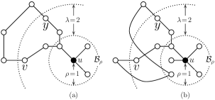
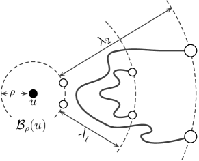
Thus high-degree nodes whose neighbors are not connected to each other have high 𝔐usubscript𝔐𝑢\mathfrak{M}_{u} values. For an intuitive interpretation and generalization of (1), the following definition of weak and strong dominance will prove useful (cf. dominating set problem for graphs GJ79 and point domination problems in geometry BDG1 ). A pair of distinct nodes v,y𝑣𝑦v,y is weakly (ρ,λ)𝜌𝜆(\rho,\lambda)-dominated (respectively, strongly (ρ,λ)𝜌𝜆(\rho,\lambda)-dominated) by a node u𝑢u provided (see Fig. 6):

  1. (a)

    ρ<du,v,du,yρ+λformulae-sequence𝜌subscript𝑑𝑢𝑣subscript𝑑𝑢𝑦𝜌𝜆\rho<d_{u,v},d_{u,y}\leq\rho+\lambda, and

  2. (b)

    for at least one shortest path 𝒫𝒫\mathcal{P} (respectively, for every shortest path 𝒫𝒫\mathcal{P}) between v𝑣v and y𝑦y, 𝒫𝒫\mathcal{P} contains a node z𝑧z such that du,zρsubscript𝑑𝑢𝑧𝜌d_{u,z}\leq\rho.

Refer to caption
Figure 6: Illustration of weak and strong domination. (a) v,y𝑣𝑦v,y is weakly (ρ,λ)𝜌𝜆(\rho,\lambda)-dominated by u𝑢u since only one shortest path between v𝑣v and y𝑦y intersects ρ(u)subscript𝜌𝑢\mathcal{B}_{\rho}(u). (b) v,y𝑣𝑦v,y is strongly (ρ,λ)𝜌𝜆(\rho,\lambda)-dominated by u𝑢u since all the shortest path between v𝑣v and y𝑦y intersect ρ(u)subscript𝜌𝑢\mathcal{B}_{\rho}(u).

Let {𝐯,𝐲}weakρ,λ𝐮 (respectively, {𝐯,𝐲}strongρ,λ𝐮superscriptsubscriptprecedesweak𝜌𝜆𝐯𝐲𝐮 (respectively, {𝐯,𝐲}strongρ,λ𝐮\mathbf{\{v,y\}\prec_{\,\mathrm{weak}}^{\,\rho,\lambda}u}\mbox{ (respectively, $\mathbf{\{v,y\}\prec_{\,\mathrm{strong}}^{\,\rho,\lambda}u}$) }

={1,if v,y is weakly (respectively, strongly)(ρ,λ)-dominated by u0,otherwiseabsentcases1if v,y is weakly (respectively, strongly)(ρ,λ)-dominated by u0otherwise\hskip 50.58878pt=\left\{\begin{array}[]{ll}1,&\!\!\begin{array}[]{l}\mbox{\small if $v,y$ is weakly (respectively, {\bf strongly})}\\ \,\,\,\,\mbox{\small$(\rho,\lambda)$-dominated by $u$}\end{array}\\[7.22743pt] 0,&\mbox{\small otherwise}\end{array}\right.

Since 1(u)=0<j 1j(u)=𝖭𝖻𝗋(u)subscript1𝑢subscript0𝑗1subscript𝑗𝑢𝖭𝖻𝗋𝑢\mathcal{B}_{1}(u)=\bigcup_{0\,<\,j\,\leq\,1}\mathcal{B}_{j}(u)=\mathsf{Nbr}(u), it follows that

𝔐u=|0<j 1j(u)|v,y 0<j 1j(u)(1{𝐯,𝐲}weak 0,𝟏𝐮)|0<j 1j(u)|subscript𝔐𝑢subscript0𝑗1subscript𝑗𝑢subscript𝑣𝑦subscript 0𝑗1subscript𝑗𝑢superscriptsubscriptprecedesweak 011𝐯𝐲𝐮subscript0𝑗1subscript𝑗𝑢\mathfrak{M}_{u}=\left|\,\cup_{0\,<\,j\,\leq\,1}\mathcal{B}_{j}(u)\,\right|\,\,-\,\,\frac{\sum_{v,y\,\in\,\bigcup_{\,0\,<\,j\,\leq\,1}\mathcal{B}_{j}(u)}\left(1-\mathbf{\{v,y\}\prec_{\,\mathrm{weak}}^{\,0,1}u}\right)}{\left|\,\cup_{0\,<\,j\,\leq\,1}\mathcal{B}_{j}(u)\,\right|}
=𝔼[ 
number of pairs of nodes v,y such that v,y is weakly (0,1)-dominated by u
 
| 
v is selected uniformly randomly from 0<j 1Bj(u)
 
]
absent𝔼delimited-[]conditional 
number of pairs of nodes v,y such that v,y is weakly (0,1)-dominated by u
 
 
v is selected uniformly randomly from 0<j 1Bj(u)
 
={\mathbb{E}}\left[\left.\text{ \begin{tabular}[]{p{1.4in}}\small number of pairs of nodes $v,y$ such that $v,y$ is {\bf weakly} $(0,1)$-dominated by $u$\end{tabular} }\right|\text{ \begin{tabular}[]{p{1.4in}}\small$v$ is selected uniformly randomly from $\bigcup_{0\,<\,j\,\leq\,1}\mathcal{B}_{j}(u)$\end{tabular} }\right]
𝔼[ 
number of pairs of nodes v,y such that v,y is strongly (0,1)-dominated by u
 
| 
v is selected uniformly randomly from 0<j 1Bj(u)
 
]
absent𝔼delimited-[]conditional 
number of pairs of nodes v,y such that v,y is strongly (0,1)-dominated by u
 
 
v is selected uniformly randomly from 0<j 1Bj(u)
 
\geq{\mathbb{E}}\left[\left.\text{ \begin{tabular}[]{p{1.4in}}\small number of pairs of nodes $v,y$ such that $v,y$ is {\bf strongly} $(0,1)$-dominated by $u$\end{tabular} }\right|\text{ \begin{tabular}[]{p{1.4in}}\small$v$ is selected uniformly randomly from $\bigcup_{0\,<\,j\,\leq\,1}\mathcal{B}_{j}(u)$\end{tabular} }\right]

and a generalization of 𝔐usubscript𝔐𝑢\mathfrak{M}_{u} is given by (replacing 0,1010,1 by ρ,λ𝜌𝜆\rho,\lambda):

𝔐u,ρ,λ=|ρ<jλj(u)|v,yρ<jλj(u)(1{𝐯,𝐲}weakρ,λ𝐮)|ρ<jλj(u)|subscript𝔐𝑢𝜌𝜆subscript𝜌𝑗𝜆subscript𝑗𝑢subscript𝑣𝑦subscript𝜌𝑗𝜆subscript𝑗𝑢superscriptsubscriptprecedesweak𝜌𝜆1𝐯𝐲𝐮subscript𝜌𝑗𝜆subscript𝑗𝑢\mathfrak{M}_{u,\rho,\lambda}=\left|\,\cup_{\rho\,<\,j\,\leq\,\lambda}\mathcal{B}_{j}(u)\,\right|\,\,-\,\,\frac{\sum_{v,y\,\in\,\bigcup_{\,\rho\,<\,j\,\leq\,\lambda}\mathcal{B}_{j}(u)}\left(1-\mathbf{\{v,y\}\prec_{\,\mathrm{weak}}^{\,\rho,\lambda}u}\right)}{\left|\,\bigcup_{\rho\,<\,j\,\leq\,\lambda}\mathcal{B}_{j}(u)\,\right|}
=𝔼[ 
number of pairs of nodes v,y such that v,y is weakly (ρ,λ)-dominated by u
 
| 
v is selected uniformly randomly from ρ<jλBj(u)
 
]
absent𝔼delimited-[]conditional 
number of pairs of nodes v,y such that v,y is weakly (ρ,λ)-dominated by u
 
 
v is selected uniformly randomly from ρ<jλBj(u)
 
={\mathbb{E}}\left[\text{ \begin{tabular}[]{p{1.4in}}\small number of pairs of nodes $v,y$ such that $v,y$ is {\bf weakly} $(\rho,\lambda)$-dominated by $u$\end{tabular} }\Bigg{|}\text{ \begin{tabular}[]{p{1.4in}}\small$v$ is selected uniformly randomly from $\cup_{\rho\,<\,j\,\leq\,\lambda}\mathcal{B}_{j}(u)$\end{tabular} }\right]
𝔼[ 
number of pairs of nodes v,y such that v,y is strongly (ρ,λ)-dominated by u
 
| 
v is selected uniformly randomly from ρ<jλBj(u)
 
]
absent𝔼delimited-[]conditional 
number of pairs of nodes v,y such that v,y is strongly (ρ,λ)-dominated by u
 
 
v is selected uniformly randomly from ρ<jλBj(u)
 
\geq{\mathbb{E}}\left[\text{ \begin{tabular}[]{p{1.4in}}\small number of pairs of nodes $v,y$ such that $v,y$ is {\bf strongly} $(\rho,\lambda)$-dominated by $u$\end{tabular} }\Bigg{|}\text{ \begin{tabular}[]{p{1.4in}}\small$v$ is selected uniformly randomly from $\cup_{\rho\,<\,j\,\leq\,\lambda}\mathcal{B}_{j}(u)$\end{tabular} }\right]

When the graph is hyperbolic (i.e., δworst+(G)subscriptsuperscript𝛿worst𝐺\delta^{+}_{\mathrm{worst}}(G) is a constant), for moderately large λ𝜆\lambda, weak and strong dominance are essentially identical and therefore weak domination has a much stronger implication. Recall that n𝑛n denotes the number of nodes in the graph G𝐺G.

Refer to caption
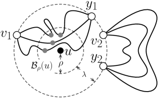
Figure 7: Visual illustration: either all the shortest paths are completely inside or all the shortest paths are completely outside of ρ+λ(u)subscript𝜌𝜆𝑢\mathcal{B}_{\rho+\lambda}(u).

Our finding can be succinctly summarized as (see Fig. 7 for a visual illustration):

(\star\!\!\!\star\!\!\!\star) If λ(6δworst+(G)+2)log2n𝜆6subscriptsuperscript𝛿worst𝐺2subscript2𝑛\lambda\geq\left(6\,\delta^{+}_{\mathrm{worst}}(G)+2\right)\log_{2}n then, assuming v𝑣v is selected uniformly randomly from ρ<jλj(u)subscript𝜌𝑗𝜆subscript𝑗𝑢\cup_{\rho\,<\,j\,\leq\,\lambda}\mathcal{B}_{j}(u) for any node u𝑢u, the expected number of pair of nodes v,y𝑣𝑦v,y that are weakly (ρ,λ)𝜌𝜆(\rho,\lambda)-dominated by u𝑢u is precisely the same as the expected number of pair of nodes that are strongly (ρ,λ)𝜌𝜆(\rho,\lambda)-dominated by u𝑢u.

Refer to caption
Figure 8: For hyperbolic graphs, the further we move from the central (black) node, the more a shortest path bends inward towards the central node.

A mathematical justification for the claim (\star\!\!\star\!\!\star) is provided by Lemma 12 in Section F of the appendix.

An implication of (\star\!\!\star\!\!\star)

If λ(6δworst+(G)+2)log2n𝜆6subscriptsuperscript𝛿worst𝐺2subscript2𝑛\lambda\geq\left(6\,\delta^{+}_{\mathrm{worst}}(G)+2\right)\log_{2}n and 𝔐u,ρ,λ|ρ+λ(u)|subscript𝔐𝑢𝜌𝜆subscript𝜌𝜆𝑢\mathfrak{M}_{u,\rho,\lambda}\approx\big{|}\,\mathcal{B}_{\rho+\lambda}(u)\,\big{|}, then almost all pairs of nodes are strongly (ρ,λ)𝜌𝜆(\rho,\lambda)-dominated by u𝑢u, i.e., for almost all pairs of nodes v,yρ+λ(u)𝑣𝑦subscript𝜌𝜆𝑢v,y\in\,\mathcal{B}_{\rho+\lambda}(u), every shortest path between v𝑣v and y𝑦y contains a node in ρ(u)subscript𝜌𝑢\mathcal{B}_{\rho}(u).

A visual illustration of this implication is in Fig. 8 showing that as λ𝜆\lambda increases the shortest paths tend to bend more and more towards the central node u𝑢u for a hyperbolic network.

Table 10: Weak domination leads to strong domination for social networks. u𝑢u is the index of the central node and
          ν=n2n1=|{(v,y)ρ+λ(u)|{𝐯,𝐲}strongρ,λ𝐮=1}||{(v,y)ρ+λ(u)|{𝐯,𝐲}weakρ,λ𝐮=1}|𝜈subscript𝑛2subscript𝑛1conditional-set𝑣𝑦subscript𝜌𝜆𝑢superscriptsubscriptprecedesstrong𝜌𝜆𝐯𝐲𝐮1conditional-set𝑣𝑦subscript𝜌𝜆𝑢superscriptsubscriptprecedesweak𝜌𝜆𝐯𝐲𝐮1\nu=\dfrac{n_{2}}{n_{1}}=\dfrac{\left|\,\left\{(v,y)\in\mathcal{B}_{\rho+\lambda}(u)\,\big{|}\,\mathbf{\{v,y\}\prec_{\,\mathrm{strong}}^{\,\rho,\lambda}u}=1\right\}\,\right|}{\left|\,\left\{(v,y)\in\mathcal{B}_{\rho+\lambda}(u)\,\big{|}\,\mathbf{\{v,y\}\prec_{\,\mathrm{weak}}^{\,\rho,\lambda}u}=1\right\}\,\right|}

[0.95] Network name u𝑢u ρ𝜌\rho λ𝜆\lambda |ρ+λ(u)|subscript𝜌𝜆𝑢\left|\,\mathcal{B}_{\rho+\lambda}(u)\,\right| ν𝜈\nu Network 1: Dolphin social network 14 4 1 5 80% 37 4 1 3 100% Network 4: Books about US politics 8 4 1 4 83% 3 3 1 5 90% Network 7: Visiting ties in San Juan 34 4 1 4 50% 9 3 1 5 90%

Empirical verification of (\star\!\!\star\!\!\star)

We empirically investigated the claim in (\star\!\!\star\!\!\star) for the following three social networks from Table 2:

Network 1

Dolphin social network,

Network 4

Books about US politics, and

Network 7

Visiting ties in San Juan.

For each network we selected a (central) node u𝑢u such that there are sufficiently many nodes in the boundary of the ξ𝜉\xi-neighborhood ξ(u)subscript𝜉𝑢\mathcal{B}_{\xi}\,(u) of u𝑢u for an appropriate ξ=ρ+λ𝜉𝜌𝜆\xi=\rho+\lambda. We then set λ𝜆\lambda to a very small value of 111, and calculated the following quantities.

  • We computed the number n1subscript𝑛1n_{1} of all pairs of nodes from ξ(u)subscript𝜉𝑢\mathcal{B}_{\xi}\,(u) that are weakly (ρ,λ)𝜌𝜆(\rho,\lambda)-dominated by u𝑢u.

  • We computed the number n2subscript𝑛2n_{2} of all pairs of nodes from ξ(u)subscript𝜉𝑢\mathcal{B}_{\xi}\,(u) that are strongly (ρ,λ)𝜌𝜆(\rho,\lambda)-dominated by u𝑢u.

Table 10 tabulates the ratio ν=n2/n1𝜈subscript𝑛2subscript𝑛1\nu=\nicefrac{{n_{2}}}{{n_{1}}}, and shows that a large percentage of the pair of nodes that were weakly dominated were also strongly dominated by u𝑢u.

IV Conclusion

In this paper we demonstrated a number of interesting properties of the shortest and approximately shortest paths in hyperbolic networks. We established the relevance of these results in the context of biological and social networks by empirically finding that a variety of such networks have close-to-tree-like topologies. Our results have important implications to a general class of directed networks which we refer to as regulatory networks. For example, our results imply that cross-talk edges or paths are frequent in these networks. Based on our theoretical results we proposed methodologies to determine relevant paths between a source and a target node in a signal transduction network, and to identify the most important nodes that mediate these paths. Our investigation shows that the hyperbolicity measure captures non-trivial topological properties that is not fully reflected in other network measures, and therefore the hyperbolicity measure should be more widely used.

Appendix A Theorem 1

Theorem 1

Suppose that G𝐺G has a cycle of k4𝑘4k\geq 4 nodes which has no path-chord. Then, δworst+(G)k/4subscriptsuperscript𝛿worst𝐺𝑘4\delta^{+}_{\mathrm{worst}}(G)\geq\left\lceil\nicefrac{{k}}{{4}}\right\rceil.

Refer to caption
Figure 9: Case 1 of Theorem 3: v=u0,1𝑣subscript𝑢01v=u_{0,1}, v=u1,2superscript𝑣subscript𝑢12v^{\prime}=u_{1,2}.

Proof.  In our proofs we will use the consequences of the 444-node condition when the 444 nodes are chosen in a specific manner as stated below in Lemma 2.

Lemma 2

Let u0,u1,u2,u3subscript𝑢0subscript𝑢1subscript𝑢2subscript𝑢3u_{0},u_{1},u_{2},u_{3} be four nodes such that u3subscript𝑢3u_{3} is on a shortest path between u1subscript𝑢1u_{1} and u2subscript𝑢2u_{2}. Suppose also that all the inter-node distances are strictly positive except for du1,u3subscript𝑑subscript𝑢1subscript𝑢3d_{u_{1},u_{3}} and du1,u3=du1,u2+du0,u1du0,u22subscript𝑑subscript𝑢1subscript𝑢3subscript𝑑subscript𝑢1subscript𝑢2subscript𝑑subscript𝑢0subscript𝑢1subscript𝑑subscript𝑢0subscript𝑢22d_{u_{1},u_{3}}=\left\lceil\frac{d_{u_{1},u_{2}}+d_{u_{0},u_{1}}-d_{u_{0},u_{2}}}{2}\right\rceil. Then,

du0,u1+du0,u2+du1,u22du0,u3+du1,u2du0,u1+du0,u2+du1,u22+2δu0,u1,u2,u3+subscript𝑑subscript𝑢0subscript𝑢1subscript𝑑subscript𝑢0subscript𝑢2subscript𝑑subscript𝑢1subscript𝑢22subscript𝑑subscript𝑢0subscript𝑢3subscript𝑑subscript𝑢1subscript𝑢2subscript𝑑subscript𝑢0subscript𝑢1subscript𝑑subscript𝑢0subscript𝑢2subscript𝑑subscript𝑢1subscript𝑢222subscriptsuperscript𝛿subscript𝑢0subscript𝑢1subscript𝑢2subscript𝑢3\left\lceil\frac{d_{u_{0},u_{1}}+d_{u_{0},u_{2}}+d_{u_{1},u_{2}}}{2}\right\rceil\leq d_{u_{0},u_{3}}+d_{u_{1},u_{2}}\\ \leq\left\lceil\frac{d_{u_{0},u_{1}}+d_{u_{0},u_{2}}+d_{u_{1},u_{2}}}{2}\right\rceil+2\,\delta^{+}_{u_{0},u_{1},u_{2},u_{3}}

Proof.  Note that due to triangle inequality 0du1,u2+du0,u1du0,u22du1,u20subscript𝑑subscript𝑢1subscript𝑢2subscript𝑑subscript𝑢0subscript𝑢1subscript𝑑subscript𝑢0subscript𝑢22subscript𝑑subscript𝑢1subscript𝑢20\leq\left\lceil\frac{d_{u_{1},u_{2}}+d_{u_{0},u_{1}}-d_{u_{0},u_{2}}}{2}\right\rceil\leq d_{u_{1},u_{2}} and thus node u3subscript𝑢3u_{3} always exists.

First, consider the case when 0<du1,u3<du1,u20subscript𝑑subscript𝑢1subscript𝑢3subscript𝑑subscript𝑢1subscript𝑢20<d_{u_{1},u_{3}}<d_{u_{1},u_{2}}. Consider the three quantities involved in the 444-node condition for the nodes u0,u1,u2,u3subscript𝑢0subscript𝑢1subscript𝑢2subscript𝑢3u_{0},u_{1},u_{2},u_{3}, namely the quantities du0,u3+du1,u2subscript𝑑subscript𝑢0subscript𝑢3subscript𝑑subscript𝑢1subscript𝑢2d_{u_{0},u_{3}}+d_{u_{1},u_{2}}, du0,u2+du1,u3subscript𝑑subscript𝑢0subscript𝑢2subscript𝑑subscript𝑢1subscript𝑢3d_{u_{0},u_{2}}+d_{u_{1},u_{3}} and du0,u1+du2,u3subscript𝑑subscript𝑢0subscript𝑢1subscript𝑑subscript𝑢2subscript𝑢3d_{u_{0},u_{1}}+d_{u_{2},u_{3}}. Note that

2(du0,u3+du1,u2)=(du0,u3+du1,u3)+(du0,u3+du2,u3)+du1,u2du0,u1+du0,u2+du1,u2du0,u3+du1,u2du0,u1+du0,u2+du1,u222subscript𝑑subscript𝑢0subscript𝑢3subscript𝑑subscript𝑢1subscript𝑢2subscript𝑑subscript𝑢0subscript𝑢3subscript𝑑subscript𝑢1subscript𝑢3subscript𝑑subscript𝑢0subscript𝑢3subscript𝑑subscript𝑢2subscript𝑢3subscript𝑑subscript𝑢1subscript𝑢2subscript𝑑subscript𝑢0subscript𝑢1subscript𝑑subscript𝑢0subscript𝑢2subscript𝑑subscript𝑢1subscript𝑢2subscript𝑑subscript𝑢0subscript𝑢3subscript𝑑subscript𝑢1subscript𝑢2subscript𝑑subscript𝑢0subscript𝑢1subscript𝑑subscript𝑢0subscript𝑢2subscript𝑑subscript𝑢1subscript𝑢222\left(d_{u_{0},u_{3}}+d_{u_{1},u_{2}}\right)=\left(d_{u_{0},u_{3}}+d_{u_{1},u_{3}}\right)+\left(d_{u_{0},u_{3}}+d_{u_{2},u_{3}}\right)+d_{u_{1},u_{2}}\\ \geq d_{u_{0},u_{1}}+d_{u_{0},u_{2}}+d_{u_{1},u_{2}}\\ \Rightarrow\,d_{u_{0},u_{3}}+d_{u_{1},u_{2}}\geq\left\lceil\frac{d_{u_{0},u_{1}}+d_{u_{0},u_{2}}+d_{u_{1},u_{2}}}{2}\right\rceil
du0,u2+du1,u3=du0,u2+du1,u2+du0,u1du0,u22=du0,u1+du0,u2+du1,u22subscript𝑑subscript𝑢0subscript𝑢2subscript𝑑subscript𝑢1subscript𝑢3subscript𝑑subscript𝑢0subscript𝑢2subscript𝑑subscript𝑢1subscript𝑢2subscript𝑑subscript𝑢0subscript𝑢1subscript𝑑subscript𝑢0subscript𝑢22subscript𝑑subscript𝑢0subscript𝑢1subscript𝑑subscript𝑢0subscript𝑢2subscript𝑑subscript𝑢1subscript𝑢22d_{u_{0},u_{2}}+d_{u_{1},u_{3}}=d_{u_{0},u_{2}}+\left\lfloor\frac{d_{u_{1},u_{2}}+d_{u_{0},u_{1}}-d_{u_{0},u_{2}}}{2}\right\rfloor\\ =\left\lfloor\frac{d_{u_{0},u_{1}}+d_{u_{0},u_{2}}+d_{u_{1},u_{2}}}{2}\right\rfloor
du0,u1+du2,u3=du0,u1+du1,u2+du0,u2du0,u12=du0,u1+du0,u2+du1,u22subscript𝑑subscript𝑢0subscript𝑢1subscript𝑑subscript𝑢2subscript𝑢3subscript𝑑subscript𝑢0subscript𝑢1subscript𝑑subscript𝑢1subscript𝑢2subscript𝑑subscript𝑢0subscript𝑢2subscript𝑑subscript𝑢0subscript𝑢12subscript𝑑subscript𝑢0subscript𝑢1subscript𝑑subscript𝑢0subscript𝑢2subscript𝑑subscript𝑢1subscript𝑢22d_{u_{0},u_{1}}+d_{u_{2},u_{3}}=d_{u_{0},u_{1}}+\left\lceil\frac{d_{u_{1},u_{2}}+d_{u_{0},u_{2}}-d_{u_{0},u_{1}}}{2}\right\rceil\\ =\left\lceil\frac{d_{u_{0},u_{1}}+d_{u_{0},u_{2}}+d_{u_{1},u_{2}}}{2}\right\rceil

Thus, du0,u3+du1,u2max{du0,u2+du1,u3,du0,u1+du2,u3}subscript𝑑subscript𝑢0subscript𝑢3subscript𝑑subscript𝑢1subscript𝑢2subscript𝑑subscript𝑢0subscript𝑢2subscript𝑑subscript𝑢1subscript𝑢3subscript𝑑subscript𝑢0subscript𝑢1subscript𝑑subscript𝑢2subscript𝑢3d_{u_{0},u_{3}}+d_{u_{1},u_{2}}\geq\max\big{\{}\,d_{u_{0},u_{2}}+d_{u_{1},u_{3}},\,d_{u_{0},u_{1}}+d_{u_{2},u_{3}}\,\big{\}} and using the definition of δu0,u1,u2,u3+subscriptsuperscript𝛿subscript𝑢0subscript𝑢1subscript𝑢2subscript𝑢3\delta^{+}_{u_{0},u_{1},u_{2},u_{3}} we have

du0,u1+du0,u2+du1,u22du0,u3+du1,u2du0,u1+du0,u2+du1,u22+2δu0,u1,u2,u3+subscript𝑑subscript𝑢0subscript𝑢1subscript𝑑subscript𝑢0subscript𝑢2subscript𝑑subscript𝑢1subscript𝑢22subscript𝑑subscript𝑢0subscript𝑢3subscript𝑑subscript𝑢1subscript𝑢2subscript𝑑subscript𝑢0subscript𝑢1subscript𝑑subscript𝑢0subscript𝑢2subscript𝑑subscript𝑢1subscript𝑢222subscriptsuperscript𝛿subscript𝑢0subscript𝑢1subscript𝑢2subscript𝑢3\left\lceil\frac{d_{u_{0},u_{1}}+d_{u_{0},u_{2}}+d_{u_{1},u_{2}}}{2}\right\rceil\leq d_{u_{0},u_{3}}+d_{u_{1},u_{2}}\\ \leq\left\lceil\frac{d_{u_{0},u_{1}}+d_{u_{0},u_{2}}+d_{u_{1},u_{2}}}{2}\right\rceil+2\,\delta^{+}_{u_{0},u_{1},u_{2},u_{3}}

Next, consider the case when du1,u3=0subscript𝑑subscript𝑢1subscript𝑢30d_{u_{1},u_{3}}=0. This implies

du0,u1+du1,u3=du0,u1+du1,u2=du0,u2=du0,u1+du0,u2+du1,u22du0,u1+du0,u2+du1,u22subscript𝑑subscript𝑢0subscript𝑢1subscript𝑑subscript𝑢1subscript𝑢3subscript𝑑subscript𝑢0subscript𝑢1subscript𝑑subscript𝑢1subscript𝑢2subscript𝑑subscript𝑢0subscript𝑢2subscript𝑑subscript𝑢0subscript𝑢1subscript𝑑subscript𝑢0subscript𝑢2subscript𝑑subscript𝑢1subscript𝑢22subscript𝑑subscript𝑢0subscript𝑢1subscript𝑑subscript𝑢0subscript𝑢2subscript𝑑subscript𝑢1subscript𝑢22d_{u_{0},u_{1}}+d_{u_{1},u_{3}}=d_{u_{0},u_{1}}+d_{u_{1},u_{2}}=d_{u_{0},u_{2}}\\ =\dfrac{d_{u_{0},u_{1}}+d_{u_{0},u_{2}}+d_{u_{1},u_{2}}}{2}\leq\left\lceil\frac{d_{u_{0},u_{1}}+d_{u_{0},u_{2}}+d_{u_{1},u_{2}}}{2}\right\rceil

Finally, consider the case when du1,u3=du1,u2subscript𝑑subscript𝑢1subscript𝑢3subscript𝑑subscript𝑢1subscript𝑢2d_{u_{1},u_{3}}=d_{u_{1},u_{2}}. This implies

du1,u2du1,u2+du0,u1du0,u22<1du0,u2+du1,u2=du0,u1+22ε for some 0<ε1subscript𝑑subscript𝑢1subscript𝑢2subscript𝑑subscript𝑢1subscript𝑢2subscript𝑑subscript𝑢0subscript𝑢1subscript𝑑subscript𝑢0subscript𝑢221subscript𝑑subscript𝑢0subscript𝑢2subscript𝑑subscript𝑢1subscript𝑢2subscript𝑑subscript𝑢0subscript𝑢122𝜀 for some 0<ε1d_{u_{1},u_{2}}-\frac{d_{u_{1},u_{2}}+d_{u_{0},u_{1}}-d_{u_{0},u_{2}}}{2}<1\\ \equiv\,d_{u_{0},u_{2}}+d_{u_{1},u_{2}}=d_{u_{0},u_{1}}+2-2\,\varepsilon\,\,\,\mbox{ for some $0<\varepsilon\leq 1$}

Thus, it easily follows that

du0,u3+du1,u2=du0,u2+du1,u2=du0,u2+du1,u2+du0,u1+22ε2=du0,u2+du1,u2+du0,u12+1εdu0,u3+du1,u2du0,u1+du0,u2+du1,u22subscript𝑑subscript𝑢0subscript𝑢3subscript𝑑subscript𝑢1subscript𝑢2subscript𝑑subscript𝑢0subscript𝑢2subscript𝑑subscript𝑢1subscript𝑢2subscript𝑑subscript𝑢0subscript𝑢2subscript𝑑subscript𝑢1subscript𝑢2subscript𝑑subscript𝑢0subscript𝑢122𝜀2subscript𝑑subscript𝑢0subscript𝑢2subscript𝑑subscript𝑢1subscript𝑢2subscript𝑑subscript𝑢0subscript𝑢121𝜀subscript𝑑subscript𝑢0subscript𝑢3subscript𝑑subscript𝑢1subscript𝑢2subscript𝑑subscript𝑢0subscript𝑢1subscript𝑑subscript𝑢0subscript𝑢2subscript𝑑subscript𝑢1subscript𝑢22d_{u_{0},u_{3}}+d_{u_{1},u_{2}}=d_{u_{0},u_{2}}+d_{u_{1},u_{2}}=\frac{d_{u_{0},u_{2}}+d_{u_{1},u_{2}}+d_{u_{0},u_{1}}+2-2\,\varepsilon}{2}\\ =\frac{d_{u_{0},u_{2}}+d_{u_{1},u_{2}}+d_{u_{0},u_{1}}}{2}+1-\varepsilon\\ \Rightarrow\,d_{u_{0},u_{3}}+d_{u_{1},u_{2}}\leq\left\lceil\frac{d_{u_{0},u_{1}}+d_{u_{0},u_{2}}+d_{u_{1},u_{2}}}{2}\right\rceil

We can now prove Theorem 1 as follows. Let 𝒞=(u0,u1,,uk1,u0)𝒞subscript𝑢0subscript𝑢1subscript𝑢𝑘1subscript𝑢0\mathcal{C}=\big{(}u_{0},u_{1},\dots,u_{k-1},u_{0}\big{)} be the cycle of k=4r+r𝑘4𝑟superscript𝑟k=4r+r^{\prime} nodes for some integers r𝑟r and 0r<40superscript𝑟40\leq r^{\prime}<4. Consider the four nodes u0,ur+r/2,u2r+(r+r/2)/ 2subscript𝑢0subscript𝑢𝑟superscript𝑟2subscript𝑢2𝑟superscript𝑟superscript𝑟22u_{0},u_{r+\left\lceil\nicefrac{{r^{\prime}}}{{2}}\right\rceil},u_{2r+\left\lfloor\,\left(\,r^{\prime}+\left\lceil\nicefrac{{r^{\prime}}}{{2}}\right\rceil\,\right)\,/\,2\,\right\rfloor} and u3r+rsubscript𝑢3𝑟superscript𝑟u_{3r+r^{\prime}}. Since 𝒞𝒞\mathcal{C} has no path-chord, we have du0,ur+r/2=r+r/2subscript𝑑subscript𝑢0subscript𝑢𝑟superscript𝑟2𝑟superscript𝑟2d_{u_{0},u_{r+\left\lceil\nicefrac{{r^{\prime}}}{{2}}\right\rceil}}=r+\left\lceil\nicefrac{{r^{\prime}}}{{2}}\right\rceil, du0,u2r+(r+r/2)/ 2=2r+r+r/22dur+r/2,u3r+r=2r+rr/22r+r/2subscript𝑑subscript𝑢0subscript𝑢2𝑟superscript𝑟superscript𝑟222𝑟superscript𝑟superscript𝑟22subscript𝑑subscript𝑢𝑟superscript𝑟2subscript𝑢3𝑟superscript𝑟2𝑟superscript𝑟superscript𝑟22𝑟superscript𝑟2d_{u_{0},u_{2r+\left\lfloor\,\left(\,r^{\prime}+\left\lceil\nicefrac{{r^{\prime}}}{{2}}\right\rceil\,\right)\,/\,2\,\right\rfloor}}=2r+\left\lfloor\,\frac{r^{\prime}+\left\lceil\nicefrac{{r^{\prime}}}{{2}}\right\rceil}{2}\,\right\rfloor d_{u_{r+\left\lceil r^{\prime}/2\right\rceil},u_{3r+r^{\prime}}}=2r+r^{\prime}-\left\lceil\nicefrac{{r^{\prime}}}{{2}}\right\rceil\leq 2r+\left\lceil\nicefrac{{r^{\prime}}}{{2}}\right\rceil, du0,u3r+r=rsubscript𝑑subscript𝑢0subscript𝑢3𝑟superscript𝑟𝑟d_{u_{0},u_{3r+r^{\prime}}}=r and u2r+(r+r/2)/ 2subscript𝑢2𝑟superscript𝑟superscript𝑟22u_{2r+\left\lfloor\,\left(\,r^{\prime}+\left\lceil\nicefrac{{r^{\prime}}}{{2}}\right\rceil\,\right)\,/\,2\,\right\rfloor} is on a shortest path between ursubscript𝑢𝑟u_{r} and u3r+rsubscript𝑢3𝑟superscript𝑟u_{3r+r^{\prime}}. Thus, applying the bound of Lemma 2, we get

δworst+(G)δu0,ur+r/2,u2r+(r+r/2)/ 2,u3r+r+du0,u2r+r+r/22+dur+r2,u3r+rdu0,ur+r2+dur+r2,u3r+r+du3r+r,u022=4r+r+r/22r+r/24r+r22=r+r+r/22r2r1/4δworst+(G)r=k/4subscriptsuperscript𝛿worst𝐺subscriptsuperscript𝛿subscript𝑢0subscript𝑢𝑟superscript𝑟2subscript𝑢2𝑟superscript𝑟superscript𝑟22subscript𝑢3𝑟superscript𝑟subscript𝑑subscript𝑢0subscript𝑢2𝑟superscript𝑟superscript𝑟22subscript𝑑subscript𝑢𝑟superscript𝑟2subscript𝑢3𝑟𝑟subscript𝑑subscript𝑢0subscript𝑢𝑟superscript𝑟2subscript𝑑subscript𝑢𝑟superscript𝑟2subscript𝑢3𝑟superscript𝑟subscript𝑑subscript𝑢3𝑟𝑟subscript𝑢0224𝑟superscript𝑟superscript𝑟22superscript𝑟superscript𝑟24𝑟superscript𝑟22𝑟superscript𝑟superscript𝑟22superscript𝑟2𝑟14subscriptsuperscript𝛿worst𝐺𝑟𝑘4\delta^{+}_{\mathrm{worst}}(G)\geq\delta^{+}_{u_{0},\,u_{r+\left\lceil\nicefrac{{r^{\prime}}}{{2}}\right\rceil},\,u_{2r+\left\lfloor\,\left(\,r^{\prime}+\left\lceil\nicefrac{{r^{\prime}}}{{2}}\right\rceil\,\right)\,/\,2\,\right\rfloor},\,u_{3r+r^{\prime}}}\\ \geq\frac{d_{u_{0},u_{2r+\left\lfloor\,\frac{r^{\prime}+\left\lceil\nicefrac{{r^{\prime}}}{{2}}\right\rceil}{2}\right\rfloor}}+d_{u_{r+\left\lceil\frac{r^{\prime}}{2}\right\rceil},u_{3r+r}}-\left\lceil\frac{d_{u_{0},u_{r+\left\lceil\frac{r^{\prime}}{2}\right\rceil}}+d_{u_{r+\left\lceil\frac{r^{\prime}}{2}\right\rceil},u_{3r+r^{\prime}}}+d_{u_{3r+r},u_{0}}}{2}\right\rceil}{2}\\ =\frac{4r+\left\lfloor\,\frac{r^{\prime}+\left\lceil\nicefrac{{r^{\prime}}}{{2}}\right\rceil}{2}\,\right\rfloor-r^{\prime}+\left\lceil\nicefrac{{r^{\prime}}}{{2}}\right\rceil-\left\lceil\dfrac{4r+r^{\prime}}{2}\right\rceil}{2}=r+\frac{\left\lfloor\,\frac{r^{\prime}+\left\lceil\nicefrac{{r^{\prime}}}{{2}}\right\rceil}{2}\,\right\rfloor-r^{\prime}}{2}\\ \geq r-\nicefrac{{1}}{{4}}\,\,\Rightarrow\,\,\delta^{+}_{\mathrm{worst}}(G)\geq r=\left\lceil\nicefrac{{k}}{{4}}\right\rceil

Appendix B Theorem 3 and Corollary 4

Refer to caption
Figure 10: A pictorial illustration of the claim in Theorem 3.

The Gromov product nodes u0,1,u0,2,u1,2subscript𝑢01subscript𝑢02subscript𝑢12u_{0,1},u_{0,2},u_{1,2} of a shortest-path triangle Δ{u0,u1,u2}subscriptΔsubscript𝑢0subscript𝑢1subscript𝑢2\Delta_{\left\{u_{0},u_{1},u_{2}\right\}} are three nodes satisfying the following555To simplify exposition, we assume that du0,u1+du1,u2+du0,u2subscript𝑑subscript𝑢0subscript𝑢1subscript𝑑subscript𝑢1subscript𝑢2subscript𝑑subscript𝑢0subscript𝑢2d_{u_{0},u_{1}}+d_{u_{1},u_{2}}+d_{u_{0},u_{2}} is an even number. Otherwise, the definition will require minor changes.:

  • u0,1subscript𝑢01u_{0,1}, u0,2subscript𝑢02u_{0,2} and u1,2subscript𝑢12u_{1,2} are located on the paths 𝒫Δ(u0,u1)subscript𝒫Δsubscript𝑢0subscript𝑢1\mathcal{P}_{\Delta}\left(u_{0},u_{1}\right), 𝒫Δ(u0,u2)subscript𝒫Δsubscript𝑢0subscript𝑢2\mathcal{P}_{\Delta}\left(u_{0},u_{2}\right) and 𝒫Δ(u1,u2)subscript𝒫Δsubscript𝑢1subscript𝑢2\mathcal{P}_{\Delta}\left(u_{1},u_{2}\right), respectively, and

  • the distances of these three nodes from u0,u1subscript𝑢0subscript𝑢1u_{0},u_{1} and u2subscript𝑢2u_{2} satisfy the following constraints:

    du0,u0,1+du1,u0,1=du0,u1,du0,u0,2+du2,u0,2=du0,u2formulae-sequencesubscript𝑑subscript𝑢0subscript𝑢01subscript𝑑subscript𝑢1subscript𝑢01subscript𝑑subscript𝑢0subscript𝑢1subscript𝑑subscript𝑢0subscript𝑢02subscript𝑑subscript𝑢2subscript𝑢02subscript𝑑subscript𝑢0subscript𝑢2\displaystyle d_{u_{0},u_{0,1}}+d_{u_{1},u_{0,1}}=d_{u_{0},u_{1}},\,\,\,\,d_{u_{0},u_{0,2}}+d_{u_{2},u_{0,2}}=d_{u_{0},u_{2}}
    du1,u1,2+du2,u1,2=du1,u2,du1,u0,1=du1,u1,2formulae-sequencesubscript𝑑subscript𝑢1subscript𝑢12subscript𝑑subscript𝑢2subscript𝑢12subscript𝑑subscript𝑢1subscript𝑢2subscript𝑑subscript𝑢1subscript𝑢01subscript𝑑subscript𝑢1subscript𝑢12\displaystyle d_{u_{1},u_{1,2}}+d_{u_{2},u_{1,2}}=d_{u_{1},u_{2}},\,\,\,\,d_{u_{1},u_{0,1}}=d_{u_{1},u_{1,2}}
    du0,u0,1=du0,u0,2=du0,u1+du0,u2du1,u22subscript𝑑subscript𝑢0subscript𝑢01subscript𝑑subscript𝑢0subscript𝑢02subscript𝑑subscript𝑢0subscript𝑢1subscript𝑑subscript𝑢0subscript𝑢2subscript𝑑subscript𝑢1subscript𝑢22\displaystyle d_{u_{0},u_{0,1}}=d_{u_{0},u_{0,2}}=\left\lfloor\dfrac{d_{u_{0},u_{1}}+d_{u_{0},u_{2}}-d_{u_{1},u_{2}}}{2}\right\rfloor

It is not difficult to see that a set of such three nodes always exists. For convenience, the nodes u1,0subscript𝑢10u_{1,0}, u2,0subscript𝑢20u_{2,0} and u2,1subscript𝑢21u_{2,1} are assumed to be the same as the nodes u0,1subscript𝑢01u_{0,1}, u0,2subscript𝑢02u_{0,2} and u1,2subscript𝑢12u_{1,2}, respectively.

Theorem 3 (see Fig. 10 for a visual illustration)

For a shortest-path triangle Δ{u0,u1,u2}subscriptΔsubscript𝑢0subscript𝑢1subscript𝑢2\Delta_{\left\{u_{0},u_{1},u_{2}\right\}} and for 0i20𝑖20\leq i\leq 2, let v𝑣v and vsuperscript𝑣v^{\prime} be two nodes on the paths ui[1.2] 𝒫Δ(ui,ui+2(mod3))ui,i+2(mod3)superscript[1.2] subscript𝒫Δsubscript𝑢𝑖subscript𝑢annotated𝑖2𝑝𝑚𝑜𝑑3subscript𝑢𝑖subscript𝑢𝑖annotated𝑖2𝑝𝑚𝑜𝑑3u_{i}\!\!\!\stackrel{{\scriptstyle\mathcal{P}_{\Delta}\left(u_{i},u_{i+2\pmod{3}}\right)}}{{\text{{[}1.2]{$\leftrightsquigarrow$} }}}\!\!\!u_{i,\,i+2\pmod{3}} and ui[1.2] 𝒫Δ(ui,ui+1(mod3))ui,i+1(mod3)superscript[1.2] subscript𝒫Δsubscript𝑢𝑖subscript𝑢annotated𝑖1𝑝𝑚𝑜𝑑3subscript𝑢𝑖subscript𝑢𝑖annotated𝑖1𝑝𝑚𝑜𝑑3u_{i}\!\!\!\stackrel{{\scriptstyle\mathcal{P}_{\Delta}\left(u_{i},u_{i+1\pmod{3}}\right)}}{{\text{{[}1.2]{$\leftrightsquigarrow$} }}}\!\!\!u_{i,\,i+1\pmod{3}}, respectively, such that dui,v=dui,vsubscript𝑑subscript𝑢𝑖𝑣subscript𝑑subscript𝑢𝑖superscript𝑣d_{u_{i},v}=d_{u_{i},v^{\prime}}. Then,

dv,v6δΔ{u0,u1,u2}++2subscript𝑑𝑣superscript𝑣6subscriptsuperscript𝛿subscriptΔsubscript𝑢0subscript𝑢1subscript𝑢22d_{v,v^{\prime}}\leq 6\,\delta^{+}_{\Delta_{\{u_{0},u_{1},u_{2}\}}}+2

where δΔ{u0,u1,u2}+δworst+(G)subscriptsuperscript𝛿subscriptΔsubscript𝑢0subscript𝑢1subscript𝑢2subscriptsuperscript𝛿worst𝐺\delta^{+}_{\Delta_{\{u_{0},u_{1},u_{2}\}}}\leq\delta^{+}_{\mathrm{worst}}(G) is the largest worst-case hyperbolicity among all combinations of four nodes in the three shortest paths defining the triangle.

Corollary 4 (Hausdorff distance between shortest paths)

Suppose that 𝒫1subscript𝒫1\mathcal{P}_{1} and 𝒫2subscript𝒫2\mathcal{P}_{2} are two shortest paths between two nodes u0subscript𝑢0u_{0} and u1subscript𝑢1u_{1}. Then, the Hausdorff distance dH(𝒫1,𝒫2)subscript𝑑𝐻subscript𝒫1subscript𝒫2d_{H}\left(\mathcal{P}_{1},\mathcal{P}_{2}\right) between these two paths can be bounded as:

dH(𝒫1,𝒫2)=defmax{maxv1𝒫1minv2𝒫2{dv1,v2},maxv2𝒫2minv1𝒫1{dv1,v2}}6δΔ{u0,u1,u2}++2superscriptdefsubscript𝑑𝐻subscript𝒫1subscript𝒫2subscriptsubscript𝑣1subscript𝒫1subscriptsubscript𝑣2subscript𝒫2subscript𝑑subscript𝑣1subscript𝑣2subscriptsubscript𝑣2subscript𝒫2subscriptsubscript𝑣1subscript𝒫1subscript𝑑subscript𝑣1subscript𝑣26subscriptsuperscript𝛿subscriptΔsubscript𝑢0subscript𝑢1subscript𝑢22\!\!\!\!\!\!\!d_{H}\left(\mathcal{P}_{1},\mathcal{P}_{2}\right)\stackrel{{\scriptstyle\mathrm{def}}}{{=}}\max\left\{\,\max_{v_{1}\,\in\,\mathcal{P}_{1}}\min_{v_{2}\,\in\,\mathcal{P}_{2}}\Big{\{}\,d_{v_{1},v_{2}}\,\Big{\}},\,\max_{v_{2}\,\in\,\mathcal{P}_{2}}\min_{v_{1}\,\in\,\mathcal{P}_{1}}\Big{\{}\,d_{v_{1},v_{2}}\,\Big{\}}\,\right\}\\ \leq 6\,\delta^{+}_{\Delta_{\{u_{0},u_{1},u_{2}\}}}+2

where u2subscript𝑢2u_{2} is any node on the path 𝒫2subscript𝒫2\mathcal{P}_{2}.

Proof of Theorem 3. To simplify exposition, we assume that du0,u1+du1,u2+du0,u2subscript𝑑subscript𝑢0subscript𝑢1subscript𝑑subscript𝑢1subscript𝑢2subscript𝑑subscript𝑢0subscript𝑢2d_{u_{0},u_{1}}+d_{u_{1},u_{2}}+d_{u_{0},u_{2}} is even and prove a slightly improve bound of dv,v6δΔ{u0,u1,u2}++1subscript𝑑𝑣superscript𝑣6subscriptsuperscript𝛿subscriptΔsubscript𝑢0subscript𝑢1subscript𝑢21d_{v,v^{\prime}}\leq 6\,\delta^{+}_{\Delta_{\{u_{0},u_{1},u_{2}\}}}+1. It is easy to modify the proof to show that dv,v6δΔ{u0,u1,u2}++2subscript𝑑𝑣superscript𝑣6subscriptsuperscript𝛿subscriptΔsubscript𝑢0subscript𝑢1subscript𝑢22d_{v,v^{\prime}}\leq 6\,\delta^{+}_{\Delta_{\{u_{0},u_{1},u_{2}\}}}+2 if du0,u1+du1,u2+du0,u2subscript𝑑subscript𝑢0subscript𝑢1subscript𝑑subscript𝑢1subscript𝑢2subscript𝑑subscript𝑢0subscript𝑢2d_{u_{0},u_{1}}+d_{u_{1},u_{2}}+d_{u_{0},u_{2}} is odd.

We will prove the result for i=1𝑖1i=1 only; similar arguments will hold for i=0𝑖0i=0 and i=2𝑖2i=2. If du1,u0,1=0subscript𝑑subscript𝑢1subscript𝑢010d_{u_{1},u_{0,1}}=0 then v=v=u1𝑣superscript𝑣subscript𝑢1v=v^{\prime}=u_{1} and the claim holds trivially, Thus, we assume that du1,u0,1>0subscript𝑑subscript𝑢1subscript𝑢010d_{u_{1},u_{0,1}}>0.

Case 1: v=u0,1𝑣subscript𝑢01{v=u_{0,1}} and v=u1,2superscript𝑣subscript𝑢12{v^{\prime}=u_{1,2}}. In this case we need to prove that du0,1,u1,26δΔ{u0,u1,u2}++1subscript𝑑subscript𝑢01subscript𝑢126subscriptsuperscript𝛿subscriptΔsubscript𝑢0subscript𝑢1subscript𝑢21d_{u_{0,1},u_{1,2}}\leq 6\,\delta^{+}_{\Delta_{\{u_{0},u_{1},u_{2}\}}}+1 (see Fig. 9). Assume that du0,1,u1,2>0subscript𝑑subscript𝑢01subscript𝑢120d_{u_{0,1},u_{1,2}}>0 since otherwise the claim is trivially true. Using Lemma 2 for the four nodes u0,u1,u2,u1,2subscript𝑢0subscript𝑢1subscript𝑢2subscript𝑢12u_{0},u_{1},u_{2},u_{1,2}, we get

du0,u1,2+du1,u2du0,u1+du1,u2+du0,u22+2δu0,u1,u2,u1,2+subscript𝑑subscript𝑢0subscript𝑢12subscript𝑑subscript𝑢1subscript𝑢2subscript𝑑subscript𝑢0subscript𝑢1subscript𝑑subscript𝑢1subscript𝑢2subscript𝑑subscript𝑢0subscript𝑢222subscriptsuperscript𝛿subscript𝑢0subscript𝑢1subscript𝑢2subscript𝑢12\displaystyle d_{u_{0},u_{1,2}}+d_{u_{1},u_{2}}\leq\left\lceil\frac{d_{u_{0},u_{1}}+d_{u_{1},u_{2}}+d_{u_{0},u_{2}}}{2}\right\rceil+2\,\delta^{+}_{u_{0},u_{1},u_{2},u_{1,2}} (2)

Now, we note that

du1,u2+du0,u0,2=du1,u2+du0,u1+du0,u2du1,u22=du0,u1+du0,u2+du1,u22subscript𝑑subscript𝑢1subscript𝑢2subscript𝑑subscript𝑢0subscript𝑢02subscript𝑑subscript𝑢1subscript𝑢2subscript𝑑subscript𝑢0subscript𝑢1subscript𝑑subscript𝑢0subscript𝑢2subscript𝑑subscript𝑢1subscript𝑢22subscript𝑑subscript𝑢0subscript𝑢1subscript𝑑subscript𝑢0subscript𝑢2subscript𝑑subscript𝑢1subscript𝑢22d_{u_{1},u_{2}}+d_{u_{0},u_{0,2}}=d_{u_{1},u_{2}}+\left\lfloor\frac{d_{u_{0},u_{1}}+d_{u_{0},u_{2}}-d_{u_{1},u_{2}}}{2}\right\rfloor\\ =\left\lfloor\frac{d_{u_{0},u_{1}}+d_{u_{0},u_{2}}+d_{u_{1},u_{2}}}{2}\right\rfloor (3)

which in turn implies

|du0,u1,2du0,u0,2|=|(du0,u1,2+du1,u2)(du1,u2+du0,u0,2)||du0,u1+du1,u2+du0,u22+2δu0,u1,u2,u1,2+(by inequality (2))du0,u1+du0,u2+du1,u22(by equality (3))|2δu0,u1,u2,u1,2++1subscript𝑑subscript𝑢0subscript𝑢12subscript𝑑subscript𝑢0subscript𝑢02subscript𝑑subscript𝑢0subscript𝑢12subscript𝑑subscript𝑢1subscript𝑢2subscript𝑑subscript𝑢1subscript𝑢2subscript𝑑subscript𝑢0subscript𝑢02subscriptsubscript𝑑subscript𝑢0subscript𝑢1subscript𝑑subscript𝑢1subscript𝑢2subscript𝑑subscript𝑢0subscript𝑢222subscriptsuperscript𝛿subscript𝑢0subscript𝑢1subscript𝑢2subscript𝑢12(by inequality (2))subscriptsubscript𝑑subscript𝑢0subscript𝑢1subscript𝑑subscript𝑢0subscript𝑢2subscript𝑑subscript𝑢1subscript𝑢22(by equality (3))2subscriptsuperscript𝛿subscript𝑢0subscript𝑢1subscript𝑢2subscript𝑢121\big{|}\,d_{u_{0},u_{1,2}}-d_{u_{0},u_{0,2}}\,\big{|}=\left|\,\left(d_{u_{0},u_{1,2}}+d_{u_{1},u_{2}}\right)-\left(d_{u_{1},u_{2}}+d_{u_{0},u_{0,2}}\right)\,\right|\\ \leq\Bigg{|}\,\,\underbrace{\left\lceil\frac{d_{u_{0},u_{1}}+d_{u_{1},u_{2}}+d_{u_{0},u_{2}}}{2}\right\rceil+2\,\delta^{+}_{u_{0},u_{1},u_{2},u_{1,2}}}_{\text{(by inequality \eqref{j6})}}\\ \hskip 93.95122pt\,-\,\underbrace{\left\lfloor\frac{d_{u_{0},u_{1}}+d_{u_{0},u_{2}}+d_{u_{1},u_{2}}}{2}\right\rfloor}_{\text{(by equality \eqref{j7})}}\,\,\Bigg{|}\\ \leq 2\,\delta^{+}_{u_{0},u_{1},u_{2},u_{1,2}}+1 (4)

In a similar manner, we can prove the following analog of inequality (4):

|du2,u0,1du2,u0,2|2δu0,u1,u2,u0,1+subscript𝑑subscript𝑢2subscript𝑢01subscript𝑑subscript𝑢2subscript𝑢022subscriptsuperscript𝛿subscript𝑢0subscript𝑢1subscript𝑢2subscript𝑢01\displaystyle\big{|}\,d_{u_{2},u_{0,1}}-d_{u_{2},u_{0,2}}\,\big{|}\leq 2\,\delta^{+}_{u_{0},u_{1},u_{2},u_{0,1}} (5)

Using inequalities (4) and (5), it follows that

|(du0,u1,2+du2,u0,1)du0,u2|=|(du0,u1,2+du2,u0,1)(du0,u0,2+du2,u0,2)|=|(du0,u1,2du0,u0,2)+(du2,u0,1du2,u0,2)||du0,u1,2du0,u0,2|+|du2,u0,1du2,u0,2|2δu0,u1,u2,u1,2++2δu0,u1,u2,u0,1++1subscript𝑑subscript𝑢0subscript𝑢12subscript𝑑subscript𝑢2subscript𝑢01subscript𝑑subscript𝑢0subscript𝑢2subscript𝑑subscript𝑢0subscript𝑢12subscript𝑑subscript𝑢2subscript𝑢01subscript𝑑subscript𝑢0subscript𝑢02subscript𝑑subscript𝑢2subscript𝑢02subscript𝑑subscript𝑢0subscript𝑢12subscript𝑑subscript𝑢0subscript𝑢02subscript𝑑subscript𝑢2subscript𝑢01subscript𝑑subscript𝑢2subscript𝑢02subscript𝑑subscript𝑢0subscript𝑢12subscript𝑑subscript𝑢0subscript𝑢02subscript𝑑subscript𝑢2subscript𝑢01subscript𝑑subscript𝑢2subscript𝑢022subscriptsuperscript𝛿subscript𝑢0subscript𝑢1subscript𝑢2subscript𝑢122subscriptsuperscript𝛿subscript𝑢0subscript𝑢1subscript𝑢2subscript𝑢011\left|\,\left(d_{u_{0},u_{1,2}}+d_{u_{2},u_{0,1}}\right)-d_{u_{0},u_{2}}\,\right|\\ =\left|\,\left(d_{u_{0},u_{1,2}}+d_{u_{2},u_{0,1}}\right)-\left(d_{u_{0},u_{0,2}}+d_{u_{2},u_{0,2}}\right)\,\right|\\ =\left|\,\left(d_{u_{0},u_{1,2}}-d_{u_{0},u_{0,2}}\right)+\left(d_{u_{2},u_{0,1}}-d_{u_{2},u_{0,2}}\right)\,\right|\\ \leq\big{|}\,d_{u_{0},u_{1,2}}-d_{u_{0},u_{0,2}}\,\big{|}\,+\,\big{|}\,d_{u_{2},u_{0,1}}-d_{u_{2},u_{0,2}}\,\big{|}\\ \leq 2\,\delta^{+}_{u_{0},u_{1},u_{2},u_{1,2}}+2\,\delta^{+}_{u_{0},u_{1},u_{2},u_{0,1}}+1 (6)

Now, consider the three quantities involved in the 444-node condition for the nodes u0,u2,u0,1,u1,2subscript𝑢0subscript𝑢2subscript𝑢01subscript𝑢12u_{0},u_{2},u_{0,1},u_{1,2}, namely the quantities: du0,u2+du0,1,u1,2subscript𝑑subscript𝑢0subscript𝑢2subscript𝑑subscript𝑢01subscript𝑢12d_{u_{0},u_{2}}+d_{u_{0,1},u_{1,2}}, du0,u1,2+du0,1,u2subscript𝑑subscript𝑢0subscript𝑢12subscript𝑑subscript𝑢01subscript𝑢2d_{u_{0},u_{1,2}}+d_{u_{0,1},u_{2}} and du0,u0,1+du2,u1,2subscript𝑑subscript𝑢0subscript𝑢01subscript𝑑subscript𝑢2subscript𝑢12d_{u_{0},u_{0,1}}+d_{u_{2},u_{1,2}}. Note that

du0,u0,1+du2,u1,2=du0,u0,2+du2,u0,2=du0,u2<du0,u2+du0,1,u1,2subscript𝑑subscript𝑢0subscript𝑢01subscript𝑑subscript𝑢2subscript𝑢12subscript𝑑subscript𝑢0subscript𝑢02subscript𝑑subscript𝑢2subscript𝑢02subscript𝑑subscript𝑢0subscript𝑢2subscript𝑑subscript𝑢0subscript𝑢2subscript𝑑subscript𝑢01subscript𝑢12\displaystyle d_{u_{0},u_{0,1}}\!\!+d_{u_{2},u_{1,2}}\!=d_{u_{0},u_{0,2}}\!\!+d_{u_{2},u_{0,2}}\!=d_{u_{0},u_{2}}\!<d_{u_{0},u_{2}}\!\!+d_{u_{0,1},u_{1,2}} (7)

If du0,u1,2+du0,1,u2du0,u0,1+du2,u1,2subscript𝑑subscript𝑢0subscript𝑢12subscript𝑑subscript𝑢01subscript𝑢2subscript𝑑subscript𝑢0subscript𝑢01subscript𝑑subscript𝑢2subscript𝑢12d_{u_{0},u_{1,2}}+d_{u_{0,1},u_{2}}\leq d_{u_{0},u_{0,1}}+d_{u_{2},u_{1,2}} then by the definition of δu0,u2,u0,1,u1,2+subscriptsuperscript𝛿subscript𝑢0subscript𝑢2subscript𝑢01subscript𝑢12\delta^{+}_{u_{0},u_{2},u_{0,1},u_{1,2}} we have

du0,1,u1,2=(du0,u2+du0,1,u1,2)du0,u2=(du0,u2+du0,1,u1,2)(du0,u0,1+du2,u1,2)2δu0,u2,u0,1,u1,2+subscript𝑑subscript𝑢01subscript𝑢12subscript𝑑subscript𝑢0subscript𝑢2subscript𝑑subscript𝑢01subscript𝑢12subscript𝑑subscript𝑢0subscript𝑢2subscript𝑑subscript𝑢0subscript𝑢2subscript𝑑subscript𝑢01subscript𝑢12subscript𝑑subscript𝑢0subscript𝑢01subscript𝑑subscript𝑢2subscript𝑢122subscriptsuperscript𝛿subscript𝑢0subscript𝑢2subscript𝑢01subscript𝑢12d_{u_{0,1},u_{1,2}}=\left(d_{u_{0},u_{2}}+d_{u_{0,1},u_{1,2}}\right)-d_{u_{0},u_{2}}\\ =\left(d_{u_{0},u_{2}}+d_{u_{0,1},u_{1,2}}\right)-\left(d_{u_{0},u_{0,1}}+d_{u_{2},u_{1,2}}\right)\leq 2\,\delta^{+}_{u_{0},u_{2},u_{0,1},u_{1,2}}

Otherwise, du0,u1,2+du0,1,u2>du0,u0,1+du2,u1,2subscript𝑑subscript𝑢0subscript𝑢12subscript𝑑subscript𝑢01subscript𝑢2subscript𝑑subscript𝑢0subscript𝑢01subscript𝑑subscript𝑢2subscript𝑢12d_{u_{0},u_{1,2}}+d_{u_{0,1},u_{2}}>d_{u_{0},u_{0,1}}+d_{u_{2},u_{1,2}} and then again by the definition of 2δu0,u2,u0,1,u1,2+2subscriptsuperscript𝛿subscript𝑢0subscript𝑢2subscript𝑢01subscript𝑢122\,\delta^{+}_{u_{0},u_{2},u_{0,1},u_{1,2}} we have

|du0,u1,2+du0,1,u2du0,u2du0,1,u1,2|2δu0,u2,u0,1,u1,2+subscript𝑑subscript𝑢0subscript𝑢12subscript𝑑subscript𝑢01subscript𝑢2subscript𝑑subscript𝑢0subscript𝑢2subscript𝑑subscript𝑢01subscript𝑢122subscriptsuperscript𝛿subscript𝑢0subscript𝑢2subscript𝑢01subscript𝑢12\left|\,d_{u_{0},u_{1,2}}+d_{u_{0,1},u_{2}}-d_{u_{0},u_{2}}-d_{u_{0,1},u_{1,2}}\,\right|\leq 2\,\delta^{+}_{u_{0},u_{2},u_{0,1},u_{1,2}}

and now using inequality (6) gives

du0,1,u1,2=(du0,u1,2+du2,u0,1du0,u2)(du0,u1,2+du0,1,u2du0,u2du0,1,u1,2)|du0,u1,2+du2,u0,1du0,u2|+|du0,u1,2+du0,1,u2du0,u2du0,1,u1,2|2δu0,u1,u2,u1,2++2δu0,u1,u2,u0,1++2δu0,u2,u0,1,u1,2++16δΔ{u0,u1,u2}++1subscript𝑑subscript𝑢01subscript𝑢12subscript𝑑subscript𝑢0subscript𝑢12subscript𝑑subscript𝑢2subscript𝑢01subscript𝑑subscript𝑢0subscript𝑢2subscript𝑑subscript𝑢0subscript𝑢12subscript𝑑subscript𝑢01subscript𝑢2subscript𝑑subscript𝑢0subscript𝑢2subscript𝑑subscript𝑢01subscript𝑢12subscript𝑑subscript𝑢0subscript𝑢12subscript𝑑subscript𝑢2subscript𝑢01subscript𝑑subscript𝑢0subscript𝑢2subscript𝑑subscript𝑢0subscript𝑢12subscript𝑑subscript𝑢01subscript𝑢2subscript𝑑subscript𝑢0subscript𝑢2subscript𝑑subscript𝑢01subscript𝑢122subscriptsuperscript𝛿subscript𝑢0subscript𝑢1subscript𝑢2subscript𝑢122subscriptsuperscript𝛿subscript𝑢0subscript𝑢1subscript𝑢2subscript𝑢012subscriptsuperscript𝛿subscript𝑢0subscript𝑢2subscript𝑢01subscript𝑢1216subscriptsuperscript𝛿subscriptΔsubscript𝑢0subscript𝑢1subscript𝑢21\!\!\!\!\!\!\!\!\!\!d_{u_{0,1},u_{1,2}}=\Big{(}d_{u_{0},u_{1,2}}+d_{u_{2},u_{0,1}}-d_{u_{0},u_{2}}\Big{)}-\Big{(}d_{u_{0},u_{1,2}}+d_{u_{0,1},u_{2}}-d_{u_{0},u_{2}}-d_{u_{0,1},u_{1,2}}\Big{)}\\ \leq\Big{|}d_{u_{0},u_{1,2}}+d_{u_{2},u_{0,1}}-d_{u_{0},u_{2}}\Big{|}+\Big{|}d_{u_{0},u_{1,2}}+d_{u_{0,1},u_{2}}-d_{u_{0},u_{2}}-d_{u_{0,1},u_{1,2}}\Big{|}\\ \leq 2\,\delta^{+}_{u_{0},u_{1},u_{2},u_{1,2}}+2\,\delta^{+}_{u_{0},u_{1},u_{2},u_{0,1}}+2\,\delta^{+}_{u_{0},u_{2},u_{0,1},u_{1,2}}+1\leq 6\,\delta^{+}_{\Delta_{\{u_{0},u_{1},u_{2}\}}}+1
Refer to caption
Figure 11: Case 2 of Theorem 3: vu0,1𝑣subscript𝑢01v\neq u_{0,1}, vu1,2superscript𝑣subscript𝑢12v^{\prime}\neq u_{1,2}.

Case 2: vu0,1𝑣subscript𝑢01{v\neq u_{0,1}} and vu1,2superscript𝑣subscript𝑢12{v^{\prime}\neq u_{1,2}}. The claim trivially holds if dv,v1subscript𝑑𝑣superscript𝑣1d_{v,v^{\prime}}\leq 1, thus we assume that dv,v>1subscript𝑑𝑣superscript𝑣1d_{v,v^{\prime}}>1. Let (v1=u1,v2=u3,v3,,vh=v,,vs=u1,2,,vr=u2)formulae-sequencesubscript𝑣1subscript𝑢1formulae-sequencesubscript𝑣2subscript𝑢3subscript𝑣3formulae-sequencesubscript𝑣superscript𝑣formulae-sequencesubscript𝑣𝑠subscript𝑢12subscript𝑣𝑟subscript𝑢2\big{(}v_{1}=u_{1},v_{2}=u_{3},v_{3},\dots,v_{h}=v^{\prime},\dots,v_{s}=u_{1,2},\dots,v_{r}=u_{2}\big{)} be the ordered sequence of nodes in the given shortest path from u1subscript𝑢1u_{1} to u2subscript𝑢2u_{2} (see Fig. 11). Consider the sequence of shortest-path triangles Δ{u0,u1,v2},Δ{u0,u1,v3},,Δ{u0,u1,vr}subscriptΔsubscript𝑢0subscript𝑢1subscript𝑣2subscriptΔsubscript𝑢0subscript𝑢1subscript𝑣3subscriptΔsubscript𝑢0subscript𝑢1subscript𝑣𝑟\Delta_{\left\{u_{0},u_{1},v_{2}\right\}},\Delta_{\left\{u_{0},u_{1},v_{3}\right\}},\dots,\Delta_{\left\{u_{0},u_{1},v_{r}\right\}}, where each such triangle Δ{u0,u1,vj}subscriptΔsubscript𝑢0subscript𝑢1subscript𝑣𝑗\Delta_{\left\{u_{0},u_{1},v_{j}\right\}} is obtained by taking the shortest path 𝒫Δ(u0,u1)subscript𝒫Δsubscript𝑢0subscript𝑢1\mathcal{P}_{\Delta}\left(u_{0},u_{1}\right), the sub-path 𝒫Δ(u1,vj)subscript𝒫Δsubscript𝑢1subscript𝑣𝑗\mathcal{P}_{\Delta}\big{(}u_{1},v_{j}\big{)} of the shortest path 𝒫Δ(u1,u2)subscript𝒫Δsubscript𝑢1subscript𝑢2\mathcal{P}_{\Delta}\left(u_{1},u_{2}\right), from u1subscript𝑢1u_{1} to vjsubscript𝑣𝑗v_{j}, and a shortest path u0𝔰vjsuperscript𝔰subscript𝑢0subscript𝑣𝑗u_{0}\!\stackrel{{\scriptstyle\mathfrak{s}}}{{\leftrightsquigarrow}}\!v_{j} from u0subscript𝑢0u_{0} to vjsubscript𝑣𝑗v_{j}. Let v1,jsubscript𝑣1𝑗v_{1,j} be the Gromov product node on the side (shortest path) 𝒫Δ(u1,vj)subscript𝒫Δsubscript𝑢1subscript𝑣𝑗\mathcal{P}_{\Delta}\big{(}u_{1},v_{j}\big{)} for the shortest-path triangle Δ{u0,u1,vj}subscriptΔsubscript𝑢0subscript𝑢1subscript𝑣𝑗\Delta_{\left\{u_{0},u_{1},v_{j}\right\}}.

We claim that if v1,j=vpsubscript𝑣1𝑗subscript𝑣𝑝v_{1,j}=v_{p} and v1,j+1=vqsubscript𝑣1𝑗1subscript𝑣𝑞v_{1,j+1}=v_{q} then q𝑞q is either p𝑝p or p+1𝑝1p+1. Indeed, if du1,vp=du0,u1+du1,ujdu0,vj2subscript𝑑subscript𝑢1subscript𝑣𝑝subscript𝑑subscript𝑢0subscript𝑢1subscript𝑑subscript𝑢1subscript𝑢𝑗subscript𝑑subscript𝑢0subscript𝑣𝑗2d_{u_{1},v_{p}}=\left\lfloor\frac{d_{u_{0},u_{1}}+d_{u_{1},u_{j}}-d_{u_{0},v_{j}}}{2}\right\rfloor and du1,vq=du0,u1+du1,uj+1du0,vj+12subscript𝑑subscript𝑢1subscript𝑣𝑞subscript𝑑subscript𝑢0subscript𝑢1subscript𝑑subscript𝑢1subscript𝑢𝑗1subscript𝑑subscript𝑢0subscript𝑣𝑗12d_{u_{1},v_{q}}=\left\lfloor\frac{d_{u_{0},u_{1}}+d_{u_{1},u_{j+1}}-d_{u_{0},v_{j+1}}}{2}\right\rfloor then

du1,vqdu1,vp=du0,u1+du1,vj+1du0,vj+12du0,u1+du1,vjdu0,vj2du0,u1+(1+du1,vj)(du0,vj+11)2du0,u1+du1,vjdu0,vj2=du0,u1+du1,vjdu0,vj2+1du0,u1+du1,vjdu0,vj21subscript𝑑subscript𝑢1subscript𝑣𝑞subscript𝑑subscript𝑢1subscript𝑣𝑝subscript𝑑subscript𝑢0subscript𝑢1subscript𝑑subscript𝑢1subscript𝑣𝑗1subscript𝑑subscript𝑢0subscript𝑣𝑗12subscript𝑑subscript𝑢0subscript𝑢1subscript𝑑subscript𝑢1subscript𝑣𝑗subscript𝑑subscript𝑢0subscript𝑣𝑗2subscript𝑑subscript𝑢0subscript𝑢11subscript𝑑subscript𝑢1subscript𝑣𝑗subscript𝑑subscript𝑢0subscript𝑣𝑗112subscript𝑑subscript𝑢0subscript𝑢1subscript𝑑subscript𝑢1subscript𝑣𝑗subscript𝑑subscript𝑢0subscript𝑣𝑗2subscript𝑑subscript𝑢0subscript𝑢1subscript𝑑subscript𝑢1subscript𝑣𝑗subscript𝑑subscript𝑢0subscript𝑣𝑗21subscript𝑑subscript𝑢0subscript𝑢1subscript𝑑subscript𝑢1subscript𝑣𝑗subscript𝑑subscript𝑢0subscript𝑣𝑗21\!\!\!\!\!\!\!\!\!\!d_{u_{1},v_{q}}-d_{u_{1},v_{p}}=\left\lfloor\frac{d_{u_{0},u_{1}}+d_{u_{1},v_{j+1}}-d_{u_{0},v_{j+1}}}{2}\right\rfloor-\left\lfloor\frac{d_{u_{0},u_{1}}+d_{u_{1},v_{j}}-d_{u_{0},v_{j}}}{2}\right\rfloor\\ \leq\left\lfloor\frac{d_{u_{0},u_{1}}+\left(1+d_{u_{1},v_{j}}\right)-\left(d_{u_{0},v_{j+1}}-1\right)}{2}\right\rfloor-\left\lfloor\frac{d_{u_{0},u_{1}}+d_{u_{1},v_{j}}-d_{u_{0},v_{j}}}{2}\right\rfloor\\ =\left\lfloor\frac{d_{u_{0},u_{1}}+d_{u_{1},v_{j}}-d_{u_{0},v_{j}}}{2}+1\right\rfloor-\left\lfloor\frac{d_{u_{0},u_{1}}+d_{u_{1},v_{j}}-d_{u_{0},v_{j}}}{2}\right\rfloor\leq 1

and a similar proof of du1,vqdu1,vp1subscript𝑑subscript𝑢1subscript𝑣𝑞subscript𝑑subscript𝑢1subscript𝑣𝑝1d_{u_{1},v_{q}}-d_{u_{1},v_{p}}\leq 1 can be obtained if du1,vp=du0,u1+du1,ujdu0,vj2subscript𝑑subscript𝑢1subscript𝑣𝑝subscript𝑑subscript𝑢0subscript𝑢1subscript𝑑subscript𝑢1subscript𝑢𝑗subscript𝑑subscript𝑢0subscript𝑣𝑗2d_{u_{1},v_{p}}=\left\lceil\frac{d_{u_{0},u_{1}}+d_{u_{1},u_{j}}-d_{u_{0},v_{j}}}{2}\right\rceil and du1,vq=du0,u1+du1,uj+1du0,vj+12subscript𝑑subscript𝑢1subscript𝑣𝑞subscript𝑑subscript𝑢0subscript𝑢1subscript𝑑subscript𝑢1subscript𝑢𝑗1subscript𝑑subscript𝑢0subscript𝑣𝑗12d_{u_{1},v_{q}}=\left\lceil\frac{d_{u_{0},u_{1}}+d_{u_{1},u_{j+1}}-d_{u_{0},v_{j+1}}}{2}\right\rceil. Thus, the ordered sequence of nodes v1,1,v1,2,,v1,rsubscript𝑣11subscript𝑣12subscript𝑣1𝑟v_{1,1},v_{1,2},\dots,v_{1,r} cover the ordered sequence of nodes v2,v3,,vssubscript𝑣2subscript𝑣3subscript𝑣𝑠v_{2},v_{3},\dots,v_{s} in a consecutive manner without skipping over any node. Since v1,1subscript𝑣11v_{1,1} is either v1subscript𝑣1v_{1} or v2subscript𝑣2v_{2}, and v1,r=vs=u1,2subscript𝑣1𝑟subscript𝑣𝑠subscript𝑢12v_{1,r}=v_{s}=u_{1,2}, there must be an index t𝑡t such that v1,t=v=vhsubscript𝑣1𝑡superscript𝑣subscript𝑣v_{1,t}=v^{\prime}=v_{h}. Since du1,v=du1,vsubscript𝑑subscript𝑢1𝑣subscript𝑑subscript𝑢1superscript𝑣d_{u_{1},v}=d_{u_{1},v^{\prime}}, v𝑣v and vsuperscript𝑣v^{\prime} are the two Gromov product nodes for the shortest-path triangle Δ{u0,u1,vt}subscriptΔsubscript𝑢0subscript𝑢1subscript𝑣𝑡\Delta_{\left\{u_{0},u_{1},v_{t}\right\}} and thus applying Case 1.1 on Δ{u0,u1,vt}subscriptΔsubscript𝑢0subscript𝑢1subscript𝑣𝑡\Delta_{\{u_{0},u_{1},v_{t}\}} we have dv,v6δΔ{u0,u1,u2}++1subscript𝑑𝑣superscript𝑣6subscriptsuperscript𝛿subscriptΔsubscript𝑢0subscript𝑢1subscript𝑢21d_{v,v^{\prime}}\leq 6\,\delta^{+}_{\Delta_{\{u_{0},u_{1},u_{2}\}}}+1. ❑

Refer to caption
Figure 12: Illustration of the bound in Theorem 5.

Appendix C Theorem 5 and Corollary 6

Theorem 5 (see Fig. 12 for a visual illustration)

Let 𝒫1u0𝔰u1subscript𝒫1subscript𝑢0superscript𝔰subscript𝑢1\mathcal{P}_{1}\equiv u_{0}\!\stackrel{{\scriptstyle\mathfrak{s}}}{{\leftrightsquigarrow}}\!u_{1} and 𝒫2subscript𝒫2\mathcal{P}_{2} be a shortest path and an arbitrary path, respectively, between two nodes u0subscript𝑢0u_{0} and u1subscript𝑢1u_{1}. Then, for every node v𝑣v on 𝒫1subscript𝒫1\mathcal{P}_{1}, there exists a node vsuperscript𝑣v^{\prime} on 𝒫2subscript𝒫2\mathcal{P}_{2} such that

dv,vmin{(6δworst+(G)+2)(log2(𝒫2)1),du0,u12}=O(δworst+(G)log(𝒫2))subscript𝑑𝑣superscript𝑣6subscriptsuperscript𝛿worst𝐺2subscript2subscript𝒫21subscript𝑑subscript𝑢0subscript𝑢12missing-subexpressionOsubscriptsuperscript𝛿worst𝐺subscript𝒫2\begin{array}[]{lcl}d_{v,v^{\prime}}&\leq&\min\left\{\,\,\Big{(}6\,\delta^{+}_{\mathrm{worst}}(G)+2\Big{)}\,\Big{(}\left\lfloor\,\log_{2}\ell\left(\mathcal{P}_{2}\right)\,\right\rfloor-1\Big{)}\,,\,\,\left\lfloor\frac{d_{u_{0},u_{1}}}{2}\right\rfloor\,\,\right\}\\[3.61371pt] &=&{\mathrm{O}\Big{(}\,\delta^{+}_{\mathrm{worst}}(G)\,\log\ell\left(\mathcal{P}_{2}\right)\Big{)}}\end{array}

Since (𝒫2)nsubscript𝒫2𝑛\ell\left(\mathcal{P}_{2}\right)\leq n, the above bound also implies that

dv,v(6δworst+(G)+2)(log2n1)=O(δworst+(G)logn)subscript𝑑𝑣superscript𝑣6subscriptsuperscript𝛿worst𝐺2subscript2𝑛1Osubscriptsuperscript𝛿worst𝐺𝑛d_{v,v^{\prime}}\leq\Big{(}6\,\delta^{+}_{\mathrm{worst}}(G)+2\Big{)}\,\Big{(}\left\lfloor\,\log_{2}n\,\right\rfloor-1\Big{)}={\mathrm{O}\Big{(}\,\delta^{+}_{\mathrm{worst}}(G)\,\log n\Big{)}}
Corollary 6

Suppose that there exists a node v𝑣v on the shortest path between u0subscript𝑢0u_{0} and u1subscript𝑢1u_{1} such that minv𝒫2{dv,v}γsubscriptsuperscript𝑣subscript𝒫2subscript𝑑𝑣superscript𝑣𝛾\min_{v^{\prime}\in\mathcal{P}_{2}}\left\{d_{v,v^{\prime}}\right\}\geq\gamma. Then, (𝒫2)2γ6δworst+(G)+2+11=Ω(2γ/δworst+(G))subscript𝒫2superscript2𝛾6subscriptsuperscript𝛿worst𝐺211Ωsuperscript2𝛾subscriptsuperscript𝛿worst𝐺\ell\left(\mathcal{P}_{2}\right)\geq 2^{{}^{\textstyle\frac{\gamma}{6\,\delta^{+}_{\mathrm{worst}}(G)+2}+1}}-1=\Omega\Big{(}2^{{}^{\textstyle\gamma\,/\,\delta^{+}_{\mathrm{worst}}(G)}}\Big{)}.

Proof of Theorem 5. First, note that by selecting vsuperscript𝑣v^{\prime} to be one of u0subscript𝑢0u_{0} or u1subscript𝑢1u_{1} appropriately we have dv,vdu0,u1/2subscript𝑑𝑣superscript𝑣subscript𝑑subscript𝑢0subscript𝑢12d_{v,v^{\prime}}\leq\left\lfloor\nicefrac{{d_{u_{0},u_{1}}}}{{2}}\right\rfloor. Now, assume that (𝒫2)>2subscript𝒫22\ell\left(\mathcal{P}_{2}\right)>2. Let u2subscript𝑢2u_{2} be the node on the path 𝒫2subscript𝒫2\mathcal{P}_{2} such that (u0𝒫2u2)=(𝒫2)/2superscriptsubscript𝒫2subscript𝑢0subscript𝑢2subscript𝒫22\ell\big{(}u_{0}\!\stackrel{{\scriptstyle\mathcal{P}_{2}}}{{\leftrightsquigarrow}}\!u_{2}\big{)}=\left\lceil\,\nicefrac{{\ell\left(\mathcal{P}_{2}\right)}}{{2}}\,\right\rceil. and consider the shortest-path triangle Δ{u0,u1,u2}subscriptΔsubscript𝑢0subscript𝑢1subscript𝑢2\Delta_{\left\{u_{0},u_{1},u_{2}\right\}}. By Theorem 3 there exists a node vsuperscript𝑣v^{\prime} either on a shortest path between u0subscript𝑢0u_{0} and u2subscript𝑢2u_{2} or on a shortest path between u1subscript𝑢1u_{1} and u2subscript𝑢2u_{2} such that dv,v6δworst+(G)+2subscript𝑑𝑣superscript𝑣6subscriptsuperscript𝛿worst𝐺2d_{v,v^{\prime}}\leq 6\,\delta^{+}_{\mathrm{worst}}(G)+2. We move from v𝑣v to vsuperscript𝑣v^{\prime} and recursively solve the problem of finding a shortest path from vsuperscript𝑣v^{\prime} to a node on a part of the path 𝒫2subscript𝒫2\mathcal{P}_{2} containing at most (𝒫2)/2subscript𝒫22\left\lceil\nicefrac{{\left(\mathcal{P}_{2}\right)}}{{2}}\right\rceil edges. Let D(y)𝐷𝑦D(y) denote the minimum distance from v𝑣v to a node in a path of length y𝑦y between u0subscript𝑢0u_{0} and u1subscript𝑢1u_{1}. Thus, the worst-case recurrence for D(y)𝐷𝑦D(y) is given by

D(y)D(y2)+6δworst+(G)+2,if y>2D(2)=1𝐷𝑦𝐷𝑦26subscriptsuperscript𝛿worst𝐺2if y>2𝐷21missing-subexpression\begin{array}[]{ll}D(y)\leq D\left(\,\left\lceil\frac{y}{2}\right\rceil\,\right)+6\,\delta^{+}_{\mathrm{worst}}(G)+2,&\mbox{if $y>2$}\\[7.22743pt] D(2)=1&\end{array}

A solution to the above recurrence satisfies D((𝒫2))(6δworst+(G)+2)(log2(𝒫2)1)𝐷subscript𝒫26subscriptsuperscript𝛿worst𝐺2subscript2subscript𝒫21D\left(\ell\left(\mathcal{P}_{2}\right)\,\right)\leq\Big{(}6\,\delta^{+}_{\mathrm{worst}}(G)+2\Big{)}\,\Big{(}\left\lceil\,\log_{2}\ell\left(\mathcal{P}_{2}\right)\,\right\rceil-1\Big{)}. ❑

Appendix D Theorem 7 and Corollary 8

For easy of display of long mathematical equations, we will denote δworst+(G)subscriptsuperscript𝛿worst𝐺\delta^{+}_{\mathrm{worst}}(G) simply as δ+superscript𝛿\delta^{+}.

Theorem 7

Let 𝒫1subscript𝒫1\mathcal{P}_{1} and 𝒫2subscript𝒫2\mathcal{P}_{2} be a shortest path and another path, respectively, between two nodes. Define η𝒫1,𝒫2subscript𝜂subscript𝒫1subscript𝒫2\eta_{\mathcal{P}_{1},\mathcal{P}_{2}} as

η𝒫1,𝒫2=(6δ++2)log2((6μ+2)(6δ++2)log2[(6δ++2)(3μ+1)μ]+μ) =O(δ+log(μδ+)), if 𝒫2 is μ-approximate shortη𝒫1,𝒫2=(6δ++2)log2(8(6δ++2)log2[(6δ++2)(4+2ε)]+1+ε2)=O(δ+log(ε+δ+logε)), if 𝒫2 is ε-additive-approximate shortsubscript𝜂subscript𝒫1subscript𝒫2=(6δ++2)log2((6μ+2)(6δ++2)log2[(6δ++2)(3μ+1)μ]+μ) absentOsuperscript𝛿𝜇superscript𝛿 if 𝒫2 is μ-approximate shortmissing-subexpressionsubscript𝜂subscript𝒫1subscript𝒫2absent6superscript𝛿2subscript286superscript𝛿2subscript26superscript𝛿242𝜀1𝜀2absentOsuperscript𝛿𝜀superscript𝛿𝜀 if 𝒫2 is ε-additive-approximate short\begin{array}[]{l}\textstyle\eta_{\,\mathcal{P}_{1},\mathcal{P}_{2}}\\ \text{\footnotesize$\textstyle=\Bigg{(}6\,\delta^{+}+2\Bigg{)}\,\log_{2}\Bigg{(}\,\bigg{(}6\,\mu+2\bigg{)}\,\bigg{(}6\,\delta^{+}+2\bigg{)}\,\log_{2}\bigg{[}\left(6\,\delta^{+}+2\right)\,\big{(}3\,\mu+1\big{)}\,\mu\bigg{]}\,+\mu\Bigg{)}$ }\\ =\mathrm{O}\left(\delta^{+}\,\log\left(\,\mu\,\delta^{+}\,\right)\,\right),\text{ if $\mathcal{P}_{2}$ is $\mu$-approximate short}\\ \\ \textstyle\eta_{\,\mathcal{P}_{1},\mathcal{P}_{2}}\\ =\textstyle\Bigg{(}6\,\delta^{+}+2\Bigg{)}\,\log_{2}\Bigg{(}8\,\bigg{(}6\,\delta^{+}+2\bigg{)}\,\log_{2}\bigg{[}\left(6\,\delta^{+}+2\right)\,\left(4+2\varepsilon\right)\bigg{]}\,+1+\dfrac{\varepsilon}{2}\Bigg{)}\\ =\mathrm{O}\left(\delta^{+}\log\Big{(}\,\varepsilon+\delta^{+}\,\log\varepsilon\,\Big{)}\,\right),\text{ if $\mathcal{P}_{2}$ is $\varepsilon$-additive-approximate short}\end{array}\vspace*{5pt}

Then, the following statements are true.

(a) For every node v𝑣v on 𝒫1subscript𝒫1\mathcal{P}_{1}, there exists a node vsuperscript𝑣v^{\prime} on 𝒫2subscript𝒫2\mathcal{P}_{2} such that dv,vη𝒫1,𝒫2subscript𝑑𝑣superscript𝑣subscript𝜂subscript𝒫1subscript𝒫2d_{v,v^{\prime}}\leq\left\lfloor\eta_{\mathcal{P}_{1},\mathcal{P}_{2}}\,\right\rfloor.

(b) For every node vsuperscript𝑣v^{\prime} on 𝒫2subscript𝒫2\mathcal{P}_{2}, there exists a node v𝑣v on 𝒫1subscript𝒫1\mathcal{P}_{1} such that dv,vζ𝒫1,𝒫2subscript𝑑𝑣superscript𝑣subscript𝜁subscript𝒫1subscript𝒫2d_{v,v^{\prime}}\leq\zeta_{\mathcal{P}_{1},\mathcal{P}_{2}} where

ζ𝒫1,𝒫2={min{(μ+1)η𝒫1,𝒫2+μ2,μdu0,u12}=O(μδ+log(μδ+)), if 𝒫2 is μ-approximate shortmin{2η𝒫1,𝒫2+1+ε2,du0,u1+ε2}=O(ε+δ+log(ε+δ+logε)), if 𝒫2 is ε-additive-approximate shortsubscript𝜁subscript𝒫1subscript𝒫2cases𝜇1subscript𝜂subscript𝒫1subscript𝒫2𝜇2𝜇subscript𝑑subscript𝑢0subscript𝑢12absentO𝜇superscript𝛿𝜇superscript𝛿 if 𝒫2 is μ-approximate short2subscript𝜂subscript𝒫1subscript𝒫21𝜀2subscript𝑑subscript𝑢0subscript𝑢1𝜀2absentO𝜀superscript𝛿𝜀superscript𝛿𝜀 if 𝒫2 is ε-additive-approximate short\zeta_{\mathcal{P}_{1},\mathcal{P}_{2}}=\left\{\begin{array}[]{l}\,\,\,\,\min\left\{\,\,\left\lfloor\big{(}\,\mu+1\,\big{)}\,\eta_{\mathcal{P}_{1},\mathcal{P}_{2}}+\dfrac{\mu}{2}\right\rfloor,\,\left\lfloor\dfrac{\mu\,d_{u_{0},u_{1}}}{2}\right\rfloor\,\,\right\}\\[7.22743pt] =\mathrm{O}\left(\mu\,\delta^{+}\,\log\left(\,\mu\,\delta^{+}\,\right)\,\right),\text{ if $\mathcal{P}_{2}$ is $\mu$-approximate short}\\[14.45377pt] \,\,\,\,\min\left\{\,\left\lfloor 2\,\eta_{\mathcal{P}_{1},\mathcal{P}_{2}}+\dfrac{1+\varepsilon}{2}\right\rfloor,\,\left\lfloor\dfrac{d_{u_{0},u_{1}}+\varepsilon}{2}\right\rfloor\,\right\}\\[7.22743pt] =\mathrm{O}\left(\varepsilon+\delta^{+}\log\left(\,\varepsilon+\delta^{+}\,\log\varepsilon\,\right)\,\right),\\[7.22743pt] \hskip 36.135pt\text{ if $\mathcal{P}_{2}$ is $\varepsilon$-additive-approximate short}\end{array}\right.
Corollary 8

(Hausdorff distance between approximate short paths) Suppose that 𝒫1subscript𝒫1\mathcal{P}_{1} and 𝒫2subscript𝒫2\mathcal{P}_{2} are two paths between two nodes. Then, the Hausdorff distance dH(𝒫1,𝒫2)subscript𝑑𝐻subscript𝒫1subscript𝒫2d_{H}\left(\mathcal{P}_{1},\mathcal{P}_{2}\right) between these two paths can be bounded as follows:

dH(𝒫1,𝒫2)=defmax{maxv1𝒫1minv2𝒫2{dv1,v2},maxv2𝒫2minv1𝒫1{dv1,v2}}η𝒫1,u0𝔰u1+ζ𝒫2,u0𝔰u1superscriptdefsubscript𝑑𝐻subscript𝒫1subscript𝒫2subscriptsubscript𝑣1subscript𝒫1subscriptsubscript𝑣2subscript𝒫2subscript𝑑subscript𝑣1subscript𝑣2subscriptsubscript𝑣2subscript𝒫2subscriptsubscript𝑣1subscript𝒫1subscript𝑑subscript𝑣1subscript𝑣2subscript𝜂superscript𝔰subscript𝒫1subscript𝑢0subscript𝑢1subscript𝜁superscript𝔰subscript𝒫2subscript𝑢0subscript𝑢1d_{H}\left(\mathcal{P}_{1},\mathcal{P}_{2}\right)\stackrel{{\scriptstyle\mathrm{def}}}{{=}}\max\left\{\,\max_{v_{1}\,\in\,\mathcal{P}_{1}}\min_{v_{2}\,\in\,\mathcal{P}_{2}}\Big{\{}\,d_{v_{1},v_{2}}\,\Big{\}},\,\max_{v_{2}\,\in\,\mathcal{P}_{2}}\min_{v_{1}\,\in\,\mathcal{P}_{1}}\Big{\{}\,d_{v_{1},v_{2}}\,\Big{\}}\,\right\}\\ \leq\eta_{\mathcal{P}_{1},\textstyle u_{0}\stackrel{{\scriptstyle\mathfrak{s}}}{{\leftrightsquigarrow}}u_{1}}+\zeta_{\mathcal{P}_{2},\textstyle u_{0}\stackrel{{\scriptstyle\mathfrak{s}}}{{\leftrightsquigarrow}}u_{1}}
Corollary 9

Suppose that there exists a node v𝑣v on the shortest path between u0subscript𝑢0u_{0} and u1subscript𝑢1u_{1} such that minv𝒫2{dv,v}γsubscriptsuperscript𝑣subscript𝒫2subscript𝑑𝑣superscript𝑣𝛾\min_{\,v^{\prime}\,\in\,\mathcal{P}_{2}}\left\{d_{v,v^{\prime}}\right\}\geq\gamma. Then, the following is true.

\bullet If 𝒫2subscript𝒫2\mathcal{P}_{2} is a μ𝜇\mu-approximate short path then

μ>2γ6δ++112γ( 24+o(1))( 6δ++1)13μ=Ω(2γ/δ+γ)𝜇superscript2𝛾6superscript𝛿112𝛾24o16superscript𝛿113𝜇Ωsuperscript2𝛾superscript𝛿𝛾\mu>\frac{2^{\textstyle\frac{\gamma}{6\,\delta^{+}+1}}}{{12\,\gamma}-\Big{(}\,24+\mathrm{o}(1)\,\Big{)}\,\Big{(}\,6\,\delta^{+}+1\,\Big{)}}-\frac{1}{3}\,\Rightarrow\,\mu=\Omega\left(\frac{2^{\textstyle\nicefrac{{\gamma}}{{\delta^{+}}}}}{\gamma}\right)

\bullet If 𝒫2subscript𝒫2\mathcal{P}_{2} is a ε𝜀\varepsilon-additive-approximate short path then

ε>2γ6δ++1(48δ++172)log2(48δ++8)ε=Ω(2γ/δ+δ+logδ+)𝜀superscript2𝛾6superscript𝛿148superscript𝛿172subscript248superscript𝛿8absent𝜀Ωsuperscript2𝛾superscript𝛿superscript𝛿superscript𝛿\begin{array}[]{l}\varepsilon\,>\,\dfrac{2^{\frac{\gamma}{6\,\delta^{+}+1}}}{\Big{(}48\,\delta^{+}\,+\frac{17}{2}\Big{)}}\,-\,\log_{2}\left(48\,\delta^{+}+8\right)\\ \hskip 28.90755pt\Rightarrow\,\varepsilon=\Omega\left(\dfrac{2^{\textstyle\nicefrac{{\gamma}}{{\delta^{+}}}}}{\delta^{+}}\,-\,\log\delta^{+}\right)\end{array}

In particular, assuming real world networks have small constant values of δ+superscript𝛿\delta^{+}, the asymptotic dependence of μ𝜇\mu and ε𝜀\varepsilon on γ𝛾\gamma can be summarized as:

both μ and ε are Ω(2cγ) for some constant 0<c<1both μ and ε are Ωsuperscript2𝑐𝛾 for some constant 0<c<1\text{both $\mu$ and $\varepsilon$ are }\Omega\left(2^{\,c\>\gamma}\,\right)\text{ for some constant $0<c<1$}

Proof of Theorem 7. Let 𝒫1subscript𝒫1\mathcal{P}_{1} and 𝒫2subscript𝒫2\mathcal{P}_{2} be a shortest path and another path, respectively, between two nodes u0subscript𝑢0u_{0} and u1subscript𝑢1u_{1}. Note that any “sub-path” of a μ𝜇\mu-approximate short path is also a μ𝜇\mu-approximately short path, i.e., ui𝒫ujsuperscript𝒫subscript𝑢𝑖subscript𝑢𝑗u_{i}\!\stackrel{{\scriptstyle\mathcal{P}}}{{\leftrightsquigarrow}}\!u_{j} is also a μ𝜇\mu-approximate short path, and similarly any sub-path of a ε𝜀\varepsilon-additive-approximate short path is also a ε𝜀\varepsilon-additive-approximate short path. μ𝜇\mu-approximate shortest paths also restrict the “span” of a path-chord of the path, i.e., if (u0,u1,,uk)subscript𝑢0subscript𝑢1subscript𝑢𝑘\big{(}u_{0},u_{1},\dots,u_{k}\big{)} is a μ𝜇\mu-approximate short path and {ui,uj}Esubscript𝑢𝑖subscript𝑢𝑗𝐸\left\{u_{i},u_{j}\right\}\in E then |ji|μ𝑗𝑖𝜇|j-i\,|\leq\mu.

(a) Let v𝑣v and vsuperscript𝑣v^{\prime} be two nodes on 𝒫1subscript𝒫1\mathcal{P}_{1} and 𝒫2subscript𝒫2\mathcal{P}_{2}, respectively, such that α=dv,v=maxv′′𝒫1minv′′′𝒫2{dv′′,v′′′}𝛼subscript𝑑𝑣superscript𝑣subscriptsuperscript𝑣′′subscript𝒫1subscriptsuperscript𝑣′′′subscript𝒫2subscript𝑑superscript𝑣′′superscript𝑣′′′\displaystyle\alpha=d_{v,v^{\prime}}=\max_{v^{\prime\prime}\in\mathcal{P}_{1}}\min_{v^{\prime\prime\prime}\in\mathcal{P}_{2}}\left\{d_{v^{\prime\prime},v^{\prime\prime\prime}}\right\}. Let vu0𝒫1vsubscript𝑣subscript𝑢0superscriptsubscript𝒫1𝑣v_{\ell}\in u_{0}\!\stackrel{{\scriptstyle\mathcal{P}_{1}}}{{\leftrightsquigarrow}}\!v and vru1𝒫1vsubscript𝑣𝑟subscript𝑢1superscriptsubscript𝒫1𝑣v_{r}\in u_{1}\!\stackrel{{\scriptstyle\mathcal{P}_{1}}}{{\leftrightsquigarrow}}\!v be two nodes defined by

dv,v=2α+1,if du0,v>2α+1du0,v,otherwisesubscript𝑑subscript𝑣𝑣2𝛼1if du0,v>2α+1subscript𝑑subscript𝑢0𝑣otherwise\displaystyle d_{v_{\ell},v}=\begin{array}[]{ll}2\,\alpha+1,&\mbox{if $d_{u_{0},v}>2\,\alpha+1$}\\ d_{u_{0},v},&\mbox{otherwise}\end{array}
dvr,v=2α+1,if du1,v>2α+1du1,v,otherwisesubscript𝑑subscript𝑣𝑟𝑣2𝛼1if du1,v>2α+1subscript𝑑subscript𝑢1𝑣otherwise\displaystyle d_{v_{r},v}=\begin{array}[]{ll}2\,\alpha+1,&\mbox{if $d_{u_{1},v}>2\,\alpha+1$}\\ d_{u_{1},v},&\mbox{otherwise}\end{array}

By definition of α𝛼\alpha, there exists two nodes v~~subscript𝑣\widetilde{v_{\ell}} and vr~~subscript𝑣𝑟\widetilde{v_{r}} on the path 𝒫2subscript𝒫2\mathcal{P}_{2} such that dv,v~,dvr,vr~αsubscript𝑑subscript𝑣~subscript𝑣subscript𝑑subscript𝑣𝑟~subscript𝑣𝑟𝛼d_{v_{\ell},\widetilde{v_{\ell}}},d_{v_{r},\widetilde{v_{r}}}\leq\alpha. Consider the 𝒫3=v~𝒫2vr~subscript𝒫3~subscript𝑣superscriptsubscript𝒫2~subscript𝑣𝑟\mathcal{P}_{3}=\widetilde{v_{\ell}}\!\stackrel{{\scriptstyle\mathcal{P}_{2}}}{{\leftrightsquigarrow}}\!\widetilde{v_{r}} that is the part of path 𝒫2subscript𝒫2\mathcal{P}_{2} from v~~subscript𝑣\widetilde{v_{\ell}} to vr~~subscript𝑣𝑟\widetilde{v_{r}}. Note that

dv~,vr~dv~,v+dv,vr+dvr,vr~6α+2subscript𝑑~subscript𝑣~subscript𝑣𝑟subscript𝑑~subscript𝑣subscript𝑣subscript𝑑subscript𝑣subscript𝑣𝑟subscript𝑑subscript𝑣𝑟~subscript𝑣𝑟6𝛼2d_{\widetilde{v_{\ell}},\widetilde{v_{r}}}\leq d_{\widetilde{v_{\ell}},{v_{\ell}}}+d_{{v_{\ell}},{v_{r}}}+d_{{v_{r}},\widetilde{v_{r}}}\leq 6\,\alpha+2

Thus, we arrive at the following inequalities

(𝒫3)(6α+2)μ,if 𝒫2 is μ-approximate short6α+2+ε,if 𝒫2 is ε-additive-approximate shortsubscript𝒫36𝛼2𝜇if 𝒫2 is μ-approximate short6𝛼2𝜀if 𝒫2 is ε-additive-approximate short\ell\left(\mathcal{P}_{3}\right)\leq\begin{array}[]{ll}\big{(}6\,\alpha+2\big{)}\,\mu,&\mbox{if $\mathcal{P}_{2}$ is $\mu$-approximate short}\\[2.168pt] 6\,\alpha+2+\varepsilon,&\mbox{if $\mathcal{P}_{2}$ is $\varepsilon$-additive-approximate short}\end{array}

Now consider the path 𝒫4=v𝔰v~𝒫2vr~𝔰vrsubscript𝒫4subscript𝑣superscript𝔰~subscript𝑣superscriptsubscript𝒫2~subscript𝑣𝑟superscript𝔰subscript𝑣𝑟\mathcal{P}_{4}=v_{\ell}\!\stackrel{{\scriptstyle\mathfrak{s}}}{{\leftrightsquigarrow}}\!\widetilde{v_{\ell}}\!\stackrel{{\scriptstyle\mathcal{P}_{2}}}{{\leftrightsquigarrow}}\!\widetilde{v_{r}}\!\stackrel{{\scriptstyle\mathfrak{s}}}{{\leftrightsquigarrow}}\!v_{r} obtained by taking a shortest path from vsubscript𝑣v_{\ell} to v~~subscript𝑣\widetilde{v_{\ell}} followed by the path 𝒫3subscript𝒫3\mathcal{P}_{3} followed by a shortest path from vrsubscript𝑣𝑟v_{r} to vr~~subscript𝑣𝑟\widetilde{v_{r}}. Note that

(𝒫4){(6α+2)μ+2α, if 𝒫2 is μ-approximate short6α+2+ε+2α=8α+2+ε,if 𝒫2 is ε-additive-approximate shortsubscript𝒫4cases6𝛼2𝜇2𝛼 if 𝒫2 is μ-approximate short6𝛼2𝜀2𝛼8𝛼2𝜀if 𝒫2 is ε-additive-approximate short\ell\left(\mathcal{P}_{4}\right)\leq\left\{\begin{array}[]{l}\big{(}6\,\alpha+2\big{)}\,\mu+2\,\alpha,\mbox{ if $\mathcal{P}_{2}$ is $\mu$-approximate short}\\[5.05942pt] 6\,\alpha+2+\varepsilon+2\,\alpha=8\,\alpha+2+\varepsilon,\\ \hskip 28.90755pt\mbox{if $\mathcal{P}_{2}$ is $\varepsilon$-additive-approximate short}\end{array}\right.

We claim that minv~𝒫4{dv,v~}=αsubscript~𝑣subscript𝒫4subscript𝑑𝑣~𝑣𝛼\min_{\,\widetilde{v}\,\in\,\mathcal{P}_{4}}\{d_{v,\widetilde{v}}\}=\alpha. Indeed, if v~𝒫3~𝑣subscript𝒫3\widetilde{v}\in\mathcal{P}_{3} then, by definition of α𝛼\alpha, minv~{dv,v~}=αsubscript~𝑣subscript𝑑𝑣~𝑣𝛼\min_{\,\widetilde{v}}\,\{d_{v,\widetilde{v}}\}=\alpha. Otherwise, if v~v𝔰v~~𝑣subscript𝑣superscript𝔰~subscript𝑣\widetilde{v}\in v_{\ell}\!\stackrel{{\scriptstyle\mathfrak{s}}}{{\leftrightsquigarrow}}\!\widetilde{v_{\ell}}, then by triangle inequality dv,vdv,v~+dv~,vdv,v~2α+1dv~,v>αsubscript𝑑subscript𝑣𝑣subscript𝑑𝑣~𝑣subscript𝑑~𝑣subscript𝑣subscript𝑑𝑣~𝑣2𝛼1subscript𝑑~𝑣subscript𝑣𝛼d_{v_{\ell},v}\leq d_{v,\widetilde{v}}+d_{\,\widetilde{v},v_{\ell}}\,\Rightarrow\,d_{v,\widetilde{v}}\geq 2\,\alpha+1-d_{\,\widetilde{v},v_{\ell}}>\alpha. Similarly, if v~vr~𝔰vr~𝑣~subscript𝑣𝑟superscript𝔰subscript𝑣𝑟\widetilde{v}\in\widetilde{v_{r}}\!\stackrel{{\scriptstyle\mathfrak{s}}}{{\leftrightsquigarrow}}\!v_{r}, then by triangle inequality dvr,vdv,v~+dv~,vrdv,v~2α+1dv~,vr>αsubscript𝑑subscript𝑣𝑟𝑣subscript𝑑𝑣~𝑣subscript𝑑~𝑣subscript𝑣𝑟subscript𝑑𝑣~𝑣2𝛼1subscript𝑑~𝑣subscript𝑣𝑟𝛼d_{v_{r},v}\leq d_{v,\widetilde{v}}+d_{\,\widetilde{v},v_{r}}\,\Rightarrow\,d_{v,\widetilde{v}}\geq 2\,\alpha+1-d_{\,\widetilde{v},v_{r}}>\alpha. Since v𝒫1vrsuperscriptsubscript𝒫1subscript𝑣subscript𝑣𝑟v_{\ell}\!\stackrel{{\scriptstyle\mathcal{P}_{1}}}{{\leftrightsquigarrow}}\!v_{r} is a shortest path between vsubscript𝑣v_{\ell} and vrsubscript𝑣𝑟v_{r} and v𝑣v is a node on this path, by Theorem 5, α(6δ++2)(log2(𝒫4)1)𝛼6superscript𝛿2subscript2subscript𝒫41\alpha\leq\left(6\,\delta^{+}+2\right)\,\left(\,\left\lfloor\,\log_{2}\ell\left(\mathcal{P}_{4}\right)\,\right\rfloor-1\right). Thus, we have the following inequalities:

\bullet If 𝒫2subscript𝒫2\mathcal{P}_{2} is a μ𝜇\mu-approximate short path then

(𝒫4)(6α+2)μ+2α=(6μ+2)α+2μ(6μ+2)(6δ++2)(log2(𝒫4)1)+2μ(6μ+2)(6δ++2)(log2((6μ+2)α+2μ)1)+2μα(6δ++2)(log2((3μ+1)α+μ))missing-subexpressionsubscript𝒫46𝛼2𝜇2𝛼6𝜇2𝛼2𝜇6𝜇26superscript𝛿2subscript2subscript𝒫412𝜇6𝜇26superscript𝛿2subscript26𝜇2𝛼2𝜇12𝜇𝛼6superscript𝛿2subscript23𝜇1𝛼𝜇\displaystyle\begin{array}[]{c l}&\ell\left(\mathcal{P}_{4}\right)\\ \leq&\big{(}6\,\alpha+2\big{)}\,\mu+2\,\alpha\\[2.168pt] =&\big{(}6\,\mu+2\big{)}\,\alpha+2\,\mu\\[2.168pt] \leq&\big{(}6\,\mu+2\big{)}\,\left(6\,\delta^{+}+2\right)\,\left(\log_{2}\ell\left(\mathcal{P}_{4}\right)-1\right)+2\,\mu\\[2.168pt] \leq&\big{(}6\,\mu+2\big{)}\,\left(6\,\delta^{+}+2\right)\,\left(\log_{2}\left(\big{(}6\,\mu+2\big{)}\,\alpha+2\,\mu\right)\,-1\right)+2\,\mu\\[2.168pt] \Rightarrow&\alpha\leq\left(6\,\delta^{+}+2\right)\,\left(\log_{2}\left(\big{(}3\,\mu+1\big{)}\,\alpha+\mu\right)\,\right)\end{array} (14)

\bullet If 𝒫2subscript𝒫2\mathcal{P}_{2} is a ε𝜀\varepsilon-additive-approximate short path then

(𝒫4)8α+2+ε8(6δ++2)(log2(𝒫4)1)+2+ε8(6δ++2)(log2(8α+2+ε)1)+2+ε8α+2+ε8(6δ++2)(log2(8α+2+ε)1)+2+εα(6δ++2)(log2(4α+1+ε2))subscript𝒫48𝛼2𝜀missing-subexpression86superscript𝛿2subscript2subscript𝒫412𝜀missing-subexpression86superscript𝛿2subscript28𝛼2𝜀12𝜀missing-subexpression8𝛼2𝜀missing-subexpressionmissing-subexpressionabsent86superscript𝛿2subscript28𝛼2𝜀12𝜀missing-subexpression𝛼6superscript𝛿2subscript24𝛼1𝜀2\displaystyle\begin{array}[]{r c l}\ell\left(\mathcal{P}_{4}\right)&\leq&8\,\alpha+2+\varepsilon\\[2.168pt] &\leq&8\,\left(6\,\delta^{+}+2\right)\,\left(\log_{2}\ell\left(\mathcal{P}_{4}\right)-1\right)+2+\varepsilon\\[2.168pt] &\leq&8\,\left(6\,\delta^{+}+2\right)\,\left(\log_{2}\left(8\,\alpha+2+\varepsilon\right)\,-1\right)+2+\varepsilon\\[2.168pt] &\Rightarrow&8\,\alpha+2+\varepsilon\\ &&\,\,\,\leq 8\,\left(6\,\delta^{+}+2\right)\,\left(\log_{2}\left(8\,\alpha+2+\varepsilon\right)\,-1\right)+2+\varepsilon\\[2.168pt] &\equiv&\alpha\leq\left(6\,\delta^{+}+2\right)\,\left(\log_{2}\left(4\,\alpha+1+\frac{\varepsilon}{2}\right)\,\right)\end{array} (21)

Both  (14) and  (21) are of the form αalog2(bα+c) 2α/abα+c𝛼𝑎subscript2𝑏𝛼𝑐superscript2𝛼𝑎𝑏𝛼𝑐\alpha\leq a\log_{2}\big{(}b\,\alpha+c\big{)}\,\equiv\,2^{\nicefrac{{\alpha}}{{a}}}\leq b\,\alpha+c where

a=6δ++21 for both (14) and (21)𝑎6superscript𝛿21 for both (14) and (21)\begin{array}[]{lcl}a&=&6\,\delta^{+}+2\geq 1\text{ for both \eqref{loglog1} and \eqref{loglog2}}\\[-10.84006pt] \end{array}
b={3μ+14for (14)4for (21)c={μ1for (14)1+ε21for (21)𝑏cases3𝜇14for (14)4for (21)𝑐cases𝜇1for (14)1𝜀21for (21)\begin{array}[]{lcllcl}b&=&\left\{\begin{array}[]{ll}3\,\mu+1\geq 4&\text{for \eqref{loglog1}}\\ 4&\text{for \eqref{loglog2}}\end{array}\right.&c&=&\left\{\begin{array}[]{ll}\mu\geq 1&\text{for \eqref{loglog1}}\\ 1+\frac{\varepsilon}{2}\geq 1&\text{for \eqref{loglog2}}\end{array}\right.\end{array}

Thus, α𝛼\alpha is at most z0subscript𝑧0z_{0} where z0subscript𝑧0z_{0} is the largest positive integer value of z𝑧z that satisfies the equation:

2z/abz+csuperscript2𝑧𝑎𝑏𝑧𝑐\displaystyle 2^{\nicefrac{{z}}{{a}}}\leq b\,z+c

In the sequel, we will use the fact that log2(xy+1)log2(x+y)subscript2𝑥𝑦1subscript2𝑥𝑦\log_{2}\big{(}x\,y+1\big{)}\geq\log_{2}\big{(}x+y\big{)} for x,y1𝑥𝑦1x,y\geq 1. This holds since

x1&y1y(x1)x1xy+1x+y𝑥1𝑦1𝑦𝑥1𝑥1𝑥𝑦1𝑥𝑦x\geq 1\,\,\&\,\,y\geq 1\,\Rightarrow\,y\,(x-1)\geq x-1\,\equiv\,x\,y+1\geq x+y

We claim that z0η=alog2(2ablog2(abc)+c)subscript𝑧0𝜂𝑎subscript22𝑎𝑏subscript2𝑎𝑏𝑐𝑐z_{0}\leq\eta=a\,\log_{2}\left(2\,a\,b\log_{2}\big{(}a\,b\,c\big{)}\,+c\right). This is verified by showing that 2η/abη+csuperscript2𝜂𝑎𝑏𝜂𝑐2^{\nicefrac{{\eta}}{{a}}}\geq b\,\eta+c as follows:

2η/a=2log2(2ablog2(abc)+c)=2ablog2(abc)+cbη+c=ab(log2(2ablog2(abc)+c))+csuperscript2𝜂𝑎superscript2subscript22𝑎𝑏subscript2𝑎𝑏𝑐𝑐2𝑎𝑏subscript2𝑎𝑏𝑐𝑐𝑏𝜂𝑐𝑎𝑏subscript22𝑎𝑏subscript2𝑎𝑏𝑐𝑐𝑐\displaystyle\begin{array}[]{r c l}2^{\nicefrac{{\eta}}{{a}}}&=&2^{\log_{2}\big{(}2\,a\,b\log_{2}\big{(}a\,b\,c\big{)}\,+c\big{)}}=2\,a\,b\,\log_{2}\big{(}a\,b\,c\big{)}\,+c\\ b\,\eta+c&=&a\,b\,\left(\log_{2}\big{(}2\,a\,b\log_{2}\big{(}a\,b\,c\big{)}\,+c\big{)}\,\right)+c\end{array}
2η/a>bη+c2ablog2(abc)+cab(log2(2ablog2(abc)+c))+c2log2(abc)log2(2ablog2(abc)+c)2log2(abc)log2(2abclog2(abc)+1)since 2ablog2(abc)1 and c1(abc)2 2abclog2(abc)+1abclog2(abc)+1missing-subexpressionsuperscript2𝜂𝑎𝑏𝜂𝑐2𝑎𝑏subscript2𝑎𝑏𝑐𝑐𝑎𝑏subscript22𝑎𝑏subscript2𝑎𝑏𝑐𝑐𝑐2subscript2𝑎𝑏𝑐subscript22𝑎𝑏subscript2𝑎𝑏𝑐𝑐2subscript2𝑎𝑏𝑐subscript22𝑎𝑏𝑐subscript2𝑎𝑏𝑐1missing-subexpressionsince 2ablog2(abc)1 and c1superscript𝑎𝑏𝑐22𝑎𝑏𝑐subscript2𝑎𝑏𝑐1𝑎𝑏𝑐subscript2𝑎𝑏𝑐1\begin{array}[]{r l}&2^{\nicefrac{{\eta}}{{a}}}>b\,\eta+c\\ \equiv&2\,a\,b\,\log_{2}\big{(}a\,b\,c\big{)}\,+c\geq a\,b\,\left(\log_{2}\big{(}2\,a\,b\log_{2}\big{(}a\,b\,c\big{)}\,+c\big{)}\,\right)+c\\ \equiv&2\,\log_{2}\big{(}a\,b\,c\big{)}\,\geq\,\log_{2}\big{(}2\,a\,b\log_{2}\big{(}a\,b\,c\big{)}\,+c\big{)}\\ \Leftarrow&2\,\log_{2}\big{(}a\,b\,c\big{)}\,\geq\,\log_{2}\left(2\,a\,b\,c\log_{2}\big{(}a\,b\,c\big{)}+1\right)\\ &\,\,\,\,\,\,\,\,\text{\small since $2\,a\,b\log_{2}\big{(}a\,b\,c\big{)}\geq 1$ and $c\geq 1$}\\ \equiv&\big{(}a\,b\,c\big{)}^{2}\,\geq\,2\,a\,b\,c\log_{2}\big{(}a\,b\,c\big{)}+1\\ \Leftarrow&a\,b\,c\,\geq\,\log_{2}\big{(}a\,b\,c\big{)}+1\end{array}

and the very last inequality holds since abc4𝑎𝑏𝑐4a\,b\,c\geq 4. Thus, we arrive at the at the following bounds:

\bullet If 𝒫2subscript𝒫2\mathcal{P}_{2} is a μ𝜇\mu-approximate short path then

η=(6δ++2)log2((6μ+2)(6δ++2)log2[(6δ++2)(3μ+1)μ]+μ)𝜂6superscript𝛿2subscript26𝜇26superscript𝛿2subscript26superscript𝛿23𝜇1𝜇𝜇\eta=\Bigg{(}6\,\delta^{+}+2\Bigg{)}\,\log_{2}\Bigg{(}\,\bigg{(}6\,\mu+2\bigg{)}\,\bigg{(}6\,\delta^{+}+2\bigg{)}\,\log_{2}\bigg{[}\left(6\,\delta^{+}+2\right)\,\big{(}3\,\mu+1\big{)}\,\mu\bigg{]}\,+\mu\Bigg{)}

\bullet If 𝒫2subscript𝒫2\mathcal{P}_{2} is a ε𝜀\varepsilon-additive-approximate short path then

η=(6δ++2)log2(8(6δ++2)log2[(6δ++2)(4+2ε)]+1+ε2)𝜂6superscript𝛿2subscript286superscript𝛿2subscript26superscript𝛿242𝜀1𝜀2\eta=\Bigg{(}6\,\delta^{+}+2\Bigg{)}\,\log_{2}\Bigg{(}8\,\bigg{(}6\,\delta^{+}+2\bigg{)}\,\log_{2}\bigg{[}\left(6\,\delta^{+}+2\right)\,\left(4+2\varepsilon\right)\,\bigg{]}\,+1+\frac{\varepsilon}{2}\,\Bigg{)}

(b) Let the ordered sequence of nodes in the path 𝒫3=v1𝒫2v1subscript𝒫3subscript𝑣1superscriptsubscript𝒫2superscriptsubscript𝑣1\mathcal{P}_{3}=v_{1}\!\stackrel{{\scriptstyle\mathcal{P}_{2}}}{{\leftrightsquigarrow}}\!v_{1}^{\prime} be a (length) maximal sequence of nodes such that:

v𝒫3:minv𝒫1{dv,v}>Z𝒫1,𝒫2:for-allsuperscript𝑣subscript𝒫3subscript𝑣subscript𝒫1subscript𝑑𝑣superscript𝑣subscript𝑍subscript𝒫1subscript𝒫2\forall\,v^{\prime}\in\mathcal{P}_{3}\colon\min_{v\,\in\,\mathcal{P}_{1}}\left\{\,d_{v,v^{\prime}}\right\}>Z_{\mathcal{P}_{1},\mathcal{P}_{2}}

Consider the following set of nodes belonging to the two paths u0𝒫2v1superscriptsubscript𝒫2subscript𝑢0subscript𝑣1u_{0}\!\stackrel{{\scriptstyle\mathcal{P}_{2}}}{{\leftrightsquigarrow}}\!v_{1} and v1𝒫2u1superscriptsubscript𝒫2superscriptsubscript𝑣1subscript𝑢1v_{1}^{\prime}\!\stackrel{{\scriptstyle\mathcal{P}_{2}}}{{\leftrightsquigarrow}}\!u_{1}:

𝒮={vu0𝒫2v1|v𝒫1:dv,v=minv′′𝒫2{dv,v′′}}𝒮r={vv1𝒫2u1|v𝒫1:dv,v=minv′′𝒫2{dv,v′′}}subscript𝒮conditional-setsuperscript𝑣subscript𝑢0superscriptsubscript𝒫2subscript𝑣1:𝑣subscript𝒫1subscript𝑑𝑣superscript𝑣subscriptsuperscript𝑣′′subscript𝒫2subscript𝑑𝑣superscript𝑣′′subscript𝒮𝑟conditional-setsuperscript𝑣superscriptsubscript𝑣1superscriptsubscript𝒫2subscript𝑢1:𝑣subscript𝒫1subscript𝑑𝑣superscript𝑣subscriptsuperscript𝑣′′subscript𝒫2subscript𝑑𝑣superscript𝑣′′\begin{array}[]{l}\mathcal{S}_{\ell}=\bigcup\left\{v^{\prime}\!\in u_{0}\!\stackrel{{\scriptstyle\mathcal{P}_{2}}}{{\leftrightsquigarrow}}\!v_{1}\,\big{|}\,\exists\,v\in\mathcal{P}_{1}\colon d_{v,v^{\prime}}=\!\min_{v^{\prime\prime}\,\in\,\mathcal{P}_{2}}\left\{\,d_{v,v^{\prime\prime}}\right\}\right\}\\ \mathcal{S}_{r}=\bigcup\left\{v^{\prime}\!\in v_{1}^{\prime}\!\stackrel{{\scriptstyle\mathcal{P}_{2}}}{{\leftrightsquigarrow}}\!u_{1}\,\big{|}\,\exists\,v\in\mathcal{P}_{1}\colon d_{v,v^{\prime}}=\!\min_{v^{\prime\prime}\,\in\,\mathcal{P}_{2}}\left\{\,d_{v,v^{\prime\prime}}\right\}\right\}\end{array}

Since u0𝒮subscript𝑢0subscript𝒮u_{0}\in\mathcal{S}_{\ell} and u1𝒮rsubscript𝑢1subscript𝒮𝑟u_{1}\in\mathcal{S}_{r}, it follows that 𝒮subscript𝒮\mathcal{S}_{\ell}\neq\emptyset and 𝒮rsubscript𝒮𝑟\mathcal{S}_{r}\neq\emptyset. Note that

{vu0𝒫1u1|v𝒮𝒮r:dv,v=minv′′𝒫2{dv,v′′}}=vu0𝒫1u1{v}conditional-set𝑣subscript𝑢0superscriptsubscript𝒫1subscript𝑢1:superscript𝑣subscript𝒮subscript𝒮𝑟subscript𝑑𝑣superscript𝑣subscriptsuperscript𝑣′′subscript𝒫2subscript𝑑𝑣superscript𝑣′′subscript𝑣subscript𝑢0superscriptsubscript𝒫1subscript𝑢1𝑣\bigcup\left\{v\in u_{0}\!\stackrel{{\scriptstyle\mathcal{P}_{1}}}{{\leftrightsquigarrow}}\!u_{1}\,\big{|}\,\exists\,v^{\prime}\in\mathcal{S}_{\ell}\cup\mathcal{S}_{r}\colon d_{v,v^{\prime}}=\!\min_{v^{\prime\prime}\,\in\,\mathcal{P}_{2}}\left\{\,d_{v,v^{\prime\prime}}\right\}\right\}=\!\!\!\!\!\bigcup_{v\,\in\,u_{0}\,\stackrel{{\scriptstyle\mathcal{P}_{1}}}{{\leftrightsquigarrow}}\,u_{1}}\!\!\!\!\!\Big{\{}\,v\,\Big{\}}

Thus, there exists two adjacent nodes v4subscript𝑣4v_{4} and v4superscriptsubscript𝑣4v_{4}^{\prime} on 𝒫1subscript𝒫1\mathcal{P}_{1} such that both dv4,v3subscript𝑑subscript𝑣4subscript𝑣3d_{v_{4},v_{3}} and dv4,v3subscript𝑑superscriptsubscript𝑣4superscriptsubscript𝑣3d_{v_{4}^{\prime},v_{3}^{\prime}} is at most Z𝒫1,𝒫2subscript𝑍subscript𝒫1subscript𝒫2Z_{\mathcal{P}_{1},\mathcal{P}_{2}}. Using triangle inequality it follows that

dv3,v3dv3,v4+dv4,v4+dv4,v3=2Z𝒫1,𝒫2+1subscript𝑑subscript𝑣3superscriptsubscript𝑣3subscript𝑑subscript𝑣3subscript𝑣4subscript𝑑subscript𝑣4superscriptsubscript𝑣4subscript𝑑superscriptsubscript𝑣4superscriptsubscript𝑣32subscript𝑍subscript𝒫1subscript𝒫21d_{v_{3},v_{3}^{\prime}}\leq d_{v_{3},v_{4}}+d_{v_{4},v_{4}^{\prime}}+d_{v_{4}^{\prime},v_{3}^{\prime}}=2\,Z_{\mathcal{P}_{1},\mathcal{P}_{2}}+1

giving the following bounds

(v3𝒫2v3){μdv3,v32μZ𝒫1,𝒫2+μ,if 𝒫2 is μ-approximate shortdv3,v3+ε2Z𝒫1,𝒫2+1+ε,if 𝒫2 is ε-additive-approximate shortsuperscriptsubscript𝒫2subscript𝑣3superscriptsubscript𝑣3cases𝜇subscript𝑑subscript𝑣3superscriptsubscript𝑣32𝜇subscript𝑍subscript𝒫1subscript𝒫2𝜇if 𝒫2 is μ-approximate shortsubscript𝑑subscript𝑣3superscriptsubscript𝑣3𝜀2subscript𝑍subscript𝒫1subscript𝒫21𝜀if 𝒫2 is ε-additive-approximate short\ell\left(v_{3}\!\stackrel{{\scriptstyle\mathcal{P}_{2}}}{{\leftrightsquigarrow}}\!v_{3}^{\prime}\right)\leq\left\{\begin{array}[]{l}\mu\,d_{v_{3},v_{3}^{\prime}}\leq 2\,\mu\,Z_{\mathcal{P}_{1},\mathcal{P}_{2}}+\mu,\\ \hskip 36.135pt\text{if $\mathcal{P}_{2}$ is $\mu$-approximate short}\\[3.61371pt] d_{v_{3},v_{3}^{\prime}}+\varepsilon\leq 2\,Z_{\mathcal{P}_{1},\mathcal{P}_{2}}+1+\varepsilon,\\ \hskip 36.135pt\text{if $\mathcal{P}_{2}$ is $\varepsilon$-additive-approximate short}\end{array}\right.

For any node vsuperscript𝑣v^{\prime} on 𝒫3subscript𝒫3\mathcal{P}_{3}, we can always use the following path to reach a node on 𝒫1subscript𝒫1\mathcal{P}_{1}:

  • if dv,v3dv,v3subscript𝑑superscript𝑣subscript𝑣3subscript𝑑superscript𝑣superscriptsubscript𝑣3d_{v^{\prime},v_{3}}\leq d_{v^{\prime},v_{3}^{\prime}} then we take the path v𝒫2v3𝔰v4superscriptsubscript𝒫2superscript𝑣subscript𝑣3superscript𝔰subscript𝑣4v^{\prime}\!\stackrel{{\scriptstyle\mathcal{P}_{2}}}{{\leftrightsquigarrow}}\!v_{3}\!\stackrel{{\scriptstyle\mathfrak{s}}}{{\leftrightsquigarrow}}\!v_{4} of length at most (v3𝒫2v3)2+Z𝒫1,𝒫2superscriptsubscript𝒫2subscript𝑣3superscriptsubscript𝑣32subscript𝑍subscript𝒫1subscript𝒫2\bigg{\lfloor}\frac{\ell\left(v_{3}\stackrel{{\scriptstyle\mathcal{P}_{2}}}{{\leftrightsquigarrow}}v_{3}^{\prime}\right)}{2}\bigg{\rfloor}+Z_{\mathcal{P}_{1},\mathcal{P}_{2}} to reach the node v=v4𝑣subscript𝑣4v=v_{4} on 𝒫1subscript𝒫1\mathcal{P}_{1};

  • otherwise we take the path v𝒫2v3𝔰v4superscriptsubscript𝒫2superscript𝑣superscriptsubscript𝑣3superscript𝔰superscriptsubscript𝑣4v^{\prime}\!\stackrel{{\scriptstyle\mathcal{P}_{2}}}{{\leftrightsquigarrow}}\!v_{3}^{\prime}\!\stackrel{{\scriptstyle\mathfrak{s}}}{{\leftrightsquigarrow}}\!v_{4}^{\prime} of length at most (v3𝒫2v3)2+Z𝒫1,𝒫2superscriptsubscript𝒫2subscript𝑣3superscriptsubscript𝑣32subscript𝑍subscript𝒫1subscript𝒫2\bigg{\lfloor}\frac{\ell\,\left(v_{3}\stackrel{{\scriptstyle\mathcal{P}_{2}}}{{\leftrightsquigarrow}}v_{3}^{\prime}\right)}{2}\bigg{\rfloor}+Z_{\mathcal{P}_{1},\mathcal{P}_{2}} to reach the node v=v4𝑣superscriptsubscript𝑣4v=v_{4}^{\prime} on 𝒫1subscript𝒫1\mathcal{P}_{1}.

This gives the following worst-case bounds for dv,vsubscript𝑑𝑣superscript𝑣d_{v,v^{\prime}}:

dv,v{(μ+1)Z𝒫1,𝒫2+μ2,if 𝒫2 is μ-approximate short2Z𝒫1,𝒫2+1+ε2,if 𝒫2 is ε-additive-approximate shortsubscript𝑑𝑣superscript𝑣cases𝜇1subscript𝑍subscript𝒫1subscript𝒫2𝜇2if 𝒫2 is μ-approximate short2subscript𝑍subscript𝒫1subscript𝒫21𝜀2if 𝒫2 is ε-additive-approximate shortd_{v,v^{\prime}}\leq\left\{\begin{array}[]{l}\left\lfloor\big{(}\,\mu+1\,\big{)}\,Z_{\mathcal{P}_{1},\mathcal{P}_{2}}+\frac{\mu}{2}\right\rfloor,\text{if $\mathcal{P}_{2}$ is $\mu$-approximate short}\\[3.61371pt] \left\lfloor 2\,Z_{\mathcal{P}_{1},\mathcal{P}_{2}}+\frac{1+\varepsilon}{2}\right\rfloor,\text{if $\mathcal{P}_{2}$ is $\varepsilon$-additive-approximate short}\end{array}\right.

Refer to caption
Figure 13: Illustration of the claims in Theorem 10 and Corollary 11.

Appendix E Theorem 10 and Corollary 11

Theorem 10 (see Fig. 13 for a visual illustration)

Suppose that we are given the following:

\bullet three integers κ4𝜅4\kappa\geq 4, α>0𝛼0\alpha>0, r>(κ21)(6δworst+(G)+2)𝑟𝜅216subscriptsuperscript𝛿worst𝐺2r>\left(\frac{\kappa}{2}-1\right)\left(6\,\delta^{+}_{\mathrm{worst}}(G)+2\right),

\bullet five nodes u0,u1,u2,u3,u4subscript𝑢0subscript𝑢1subscript𝑢2subscript𝑢3subscript𝑢4u_{0},u_{1},u_{2},u_{3},u_{4} such that

  • u1,u2Br(u0)subscript𝑢1subscript𝑢2subscript𝐵𝑟subscript𝑢0u_{1},u_{2}\in B_{r}\left(u_{0}\right) with du1,u2κ2(6δworst+(G)+2)subscript𝑑subscript𝑢1subscript𝑢2𝜅26subscriptsuperscript𝛿worst𝐺2d_{u_{1},u_{2}}\geq\frac{\kappa}{2}\,\left(6\,\delta^{+}_{\mathrm{worst}}(G)+2\right),

  • du1,u4=du2,u3=αsubscript𝑑subscript𝑢1subscript𝑢4subscript𝑑subscript𝑢2subscript𝑢3𝛼d_{u_{1},u_{4}}=d_{u_{2},u_{3}}=\alpha.

Then, the following statements are true for any shortest path 𝒫𝒫\mathcal{P} between u3subscript𝑢3u_{3} and u4subscript𝑢4u_{4}:

(a) there exists a node v𝑣v on 𝒫𝒫\mathcal{P} such that

du0,vr(3κ212)(6δworst+(G)+2)=rO(κδworst+(G))subscript𝑑subscript𝑢0𝑣𝑟3𝜅2126subscriptsuperscript𝛿worst𝐺2𝑟O𝜅subscriptsuperscript𝛿worst𝐺d_{u_{0},v}\leq r-\left(\frac{3\kappa-2}{12}\right)\left(6\,\delta^{+}_{\mathrm{worst}}(G)+2\right)=r-\mathrm{O}\Big{(}\kappa\,\delta^{+}_{\mathrm{worst}}(G)\Big{)}

(b) (𝒫)(3κ26)(6δworst+(G)+2)+2α=Ω(κδworst+(G)+α)𝒫3𝜅266subscriptsuperscript𝛿worst𝐺22𝛼Ω𝜅subscriptsuperscript𝛿worst𝐺𝛼\ell\left(\mathcal{P}\right)\geq\left(\frac{3\kappa-2}{6}\right)\left(6\,\delta^{+}_{\mathrm{worst}}(G)+2\right)+2\,\alpha={\Omega\,\Big{(}\kappa\,\delta^{+}_{\mathrm{worst}}(G)\,+\,\alpha\Big{)}}.

Corollary 11 (see Fig. 13 for a visual illustration)

Consider any path 𝒬𝒬\mathcal{Q} between u3subscript𝑢3u_{3} and u4subscript𝑢4u_{4} that does not involve a node in rrr(u0)subscriptsuperscript𝑟𝑟subscriptsuperscript𝑟subscript𝑢0\cup_{r^{\prime}\leq r}\mathcal{B}_{r^{\prime}}\left(u_{0}\right). Then, the following statements hold:

(i)

(𝒬)2α6δworst+(G)+2+κ4+561=2Ω(αδworst+(G)+κ)𝒬superscript2𝛼6subscriptsuperscript𝛿worst𝐺2𝜅4561superscript2Ω𝛼subscriptsuperscript𝛿worst𝐺𝜅\ell\left(\mathcal{Q}\right)\geq 2^{{}^{\textstyle\frac{\alpha}{6\,\delta^{+}_{\mathrm{worst}}(G)+2}+\frac{\kappa}{4}+\frac{5}{6}}}-1=2^{\textstyle\Omega\,\left(\frac{\alpha}{\delta^{+}_{\mathrm{worst}}(G)}\,+\,\kappa\right)}. In particular, if δworst+(G)subscriptsuperscript𝛿worst𝐺\delta^{+}_{\mathrm{worst}}(G) is a constant then (𝒬)=2Ω(α+κ)𝒬superscript2Ω𝛼𝜅\ell\left(\mathcal{Q}\right)={2^{\textstyle\Omega\left(\alpha+\kappa\right)}} and thus (𝒬)𝒬\ell\left(\mathcal{Q}\right) increases at least exponentially with both α𝛼\alpha and κ𝜅\kappa.

(ii)

if 𝒬𝒬\mathcal{Q} is a μ𝜇\mu-approximate short path then

μ2α6δworst+(G)+2+κ41612α+(3κ26o(1))(6δworst+(G)+2)13=Ω(2Θ(αδworst+(G)+κ)α+κδworst+(G))𝜇superscript2𝛼6subscriptsuperscript𝛿worst𝐺2𝜅41612𝛼3𝜅26o16subscriptsuperscript𝛿worst𝐺213Ωsuperscript2Θ𝛼subscriptsuperscript𝛿worst𝐺𝜅𝛼𝜅subscriptsuperscript𝛿worst𝐺\mu\,\geq\,\frac{2^{\textstyle\frac{\alpha}{6\,\delta^{+}_{\mathrm{worst}}(G)+2}+\frac{\kappa}{4}-\frac{1}{6}}}{{12\,\alpha+\big{(}3\,\kappa-26-\mathrm{o}(1)\,\big{)}\,\big{(}6\,\delta^{+}_{\mathrm{worst}}(G)+2\big{)}}}-\frac{1}{3}=\Omega\left(\frac{2^{\Theta\,\left(\frac{\alpha}{\delta^{+}_{\mathrm{worst}}(G)}\,+\,\kappa\right)}}{\alpha+\kappa\,\delta^{+}_{\mathrm{worst}}(G)}\right)

In particular, if δworst+(G)subscriptsuperscript𝛿worst𝐺\delta^{+}_{\mathrm{worst}}(G) is a constant then μ=Ω(2Θ(α+κ)α+κ)𝜇Ωsuperscript2Θ𝛼𝜅𝛼𝜅\mu={\Omega\left(\frac{2^{\,\Theta\,(\alpha+\kappa)}}{\alpha+\kappa}\right)} and thus μ𝜇\mu increases at least exponentially with both α𝛼\alpha and κ𝜅\kappa.

(iii)

if 𝒬𝒬\mathcal{Q} is a ε𝜀\varepsilon-additive-approximate short path then

ε>2α6δworst+(G)+2+κ41648δworst+(G)+172log2(48δworst+(G)+16)𝜀superscript2𝛼6subscriptsuperscript𝛿worst𝐺2𝜅41648subscriptsuperscript𝛿worst𝐺172subscript248subscriptsuperscript𝛿worst𝐺16\varepsilon>\frac{2^{\textstyle\frac{\alpha}{6\,\delta^{+}_{\mathrm{worst}}(G)+2}+\frac{\kappa}{4}-\frac{1}{6}}}{48\,\delta^{+}_{\mathrm{worst}}(G)\,+\frac{17}{2}}\,-\,\log_{2}\left(48\,\delta^{+}_{\mathrm{worst}}(G)+16\right)

In particular, if δworst+(G)subscriptsuperscript𝛿worst𝐺\delta^{+}_{\mathrm{worst}}(G) is a constant then ε=Ω(2Θ(α+κ))𝜀Ωsuperscript2Θ𝛼𝜅\varepsilon={\Omega\left(2^{\,\Theta\,(\alpha+\kappa)}\right)} and thus ε𝜀\varepsilon increases at least exponentially with both α𝛼\alpha and κ𝜅\kappa.

E.1 Proof of Theorem 10

Consider the shortest-path triangle Δ{u0,u3,u4}subscriptΔsubscript𝑢0subscript𝑢3subscript𝑢4\Delta_{\left\{u_{0},u_{3},u_{4}\right\}} and let u0,3,u0,4subscript𝑢03subscript𝑢04u_{0,3},u_{0,4} and u3,4subscript𝑢34u_{3,4} be the Gromov product nodes of Δ{u0,u3,u4}subscriptΔsubscript𝑢0subscript𝑢3subscript𝑢4\Delta_{\{u_{0},u_{3},u_{4}\}} on the sides (shortest paths) u0subscript𝑢0u_{0} to u3subscript𝑢3u_{3}, u0subscript𝑢0u_{0} to u4subscript𝑢4u_{4} and u3subscript𝑢3u_{3} to u4subscript𝑢4u_{4}, respectively. Thus, du0,u0,3=du0,u0,4subscript𝑑subscript𝑢0subscript𝑢03subscript𝑑subscript𝑢0subscript𝑢04d_{u_{0},u_{0,3}}=d_{u_{0},u_{0,4}}, and β=du3,u3,4=du0,u3+du3,u4du0,u42=du3,u42𝛽subscript𝑑subscript𝑢3subscript𝑢34subscript𝑑subscript𝑢0subscript𝑢3subscript𝑑subscript𝑢3subscript𝑢4subscript𝑑subscript𝑢0subscript𝑢42subscript𝑑subscript𝑢3subscript𝑢42\beta=d_{u_{3},u_{3,4}}=\left\lfloor\frac{d_{u_{0},u_{3}}+d_{u_{3},u_{4}}-d_{u_{0},u_{4}}}{2}\right\rfloor=\left\lfloor\frac{d_{u_{3},u_{4}}}{2}\right\rfloor since du0,u3=du0,u4=r+αsubscript𝑑subscript𝑢0subscript𝑢3subscript𝑑subscript𝑢0subscript𝑢4𝑟𝛼d_{u_{0},u_{3}}=d_{u_{0},u_{4}}=r+\alpha.

We first claim that du0,u0,3<r=du0,u2subscript𝑑subscript𝑢0subscript𝑢03𝑟subscript𝑑subscript𝑢0subscript𝑢2d_{u_{0},u_{0,3}}<r=d_{u_{0},u_{2}}. Suppose for the sake of contradiction that du0,u0,3=du0,u0,4rsubscript𝑑subscript𝑢0subscript𝑢03subscript𝑑subscript𝑢0subscript𝑢04𝑟d_{u_{0},u_{0,3}}=d_{u_{0},u_{0,4}}\geq r. Then, by Theorem 3 we get du1,u26δworst+(G)+2subscript𝑑subscript𝑢1subscript𝑢26subscriptsuperscript𝛿worst𝐺2d_{u_{1},u_{2}}\leq 6\,\delta^{+}_{\mathrm{worst}}(G)+2 which contradicts the assumption that du1,u2κ2(6δworst+(G)+2)subscript𝑑subscript𝑢1subscript𝑢2𝜅26subscriptsuperscript𝛿worst𝐺2d_{u_{1},u_{2}}\geq\frac{\kappa}{2}\,\left(6\,\delta^{+}_{\mathrm{worst}}(G)+2\right) since κ4𝜅4\kappa\geq 4.

Thus, assume that du0,u0,3=du0,u0,4=rxsubscript𝑑subscript𝑢0subscript𝑢03subscript𝑑subscript𝑢0subscript𝑢04𝑟𝑥d_{u_{0},u_{0,3}}=d_{u_{0},u_{0,4}}=r-x for some integer x>0𝑥0x>0. By Theorem 3, du0,3,u0,46δworst+(G)+2subscript𝑑subscript𝑢03subscript𝑢046subscriptsuperscript𝛿worst𝐺2d_{u_{0,3},u_{0,4}}\leq 6\,\delta^{+}_{\mathrm{worst}}(G)+2. Let du0,3,u0,4=6δworst+(G)+2ysubscript𝑑subscript𝑢03subscript𝑢046subscriptsuperscript𝛿worst𝐺2𝑦d_{u_{0,3},u_{0,4}}=6\,\delta^{+}_{\mathrm{worst}}(G)+2-y for some integer 0<y6δworst+(G)+20𝑦6subscriptsuperscript𝛿worst𝐺20<y\leq 6\,\delta^{+}_{\mathrm{worst}}(G)+2 and du1,u2=κ2(6δworst+(G)+2)+zsubscript𝑑subscript𝑢1subscript𝑢2𝜅26subscriptsuperscript𝛿worst𝐺2𝑧d_{u_{1},u_{2}}=\frac{\kappa}{2}\,\left(6\,\delta^{+}_{\mathrm{worst}}(G)+2\right)+z for some integer z0𝑧0z\geq 0. Consider the 444-node condition for the four nodes u1,u2,u0,3,u0,4subscript𝑢1subscript𝑢2subscript𝑢03subscript𝑢04u_{1},u_{2},u_{0,3},u_{0,4}. The three relevant quantities for comparison are:

q=du1,u2+du0,3,u0,4=(κ2+1)(6δworst+(G)+1)+zyq==du0,3,u2+du0,4,u1=(du0,u2du0,u0,3)+(du0,u1du0,u0,4)=2xq\varparallelinv=du0,3,u1+du0,4,u2(du0,3,u0,4+du0,4,u1)+(du0,3,u0,4+du0,3,u2)=12δworst+(G)+42y+2xsubscript𝑞parallel-tosubscript𝑑subscript𝑢1subscript𝑢2subscript𝑑subscript𝑢03subscript𝑢04𝜅216subscriptsuperscript𝛿worst𝐺1𝑧𝑦subscript𝑞subscript𝑑subscript𝑢03subscript𝑢2subscript𝑑subscript𝑢04subscript𝑢1subscript𝑑subscript𝑢0subscript𝑢2subscript𝑑subscript𝑢0subscript𝑢03subscript𝑑subscript𝑢0subscript𝑢1subscript𝑑subscript𝑢0subscript𝑢042𝑥subscript𝑞\varparallelinvsubscript𝑑subscript𝑢03subscript𝑢1subscript𝑑subscript𝑢04subscript𝑢2subscript𝑑subscript𝑢03subscript𝑢04subscript𝑑subscript𝑢04subscript𝑢1subscript𝑑subscript𝑢03subscript𝑢04subscript𝑑subscript𝑢03subscript𝑢2absent12subscriptsuperscript𝛿worst𝐺42𝑦2𝑥\begin{array}[]{l}q_{\parallel}=d_{u_{1},u_{2}}+d_{u_{0,3},u_{0,4}}=\left(\frac{\kappa}{2}+1\right)\left(6\,\delta^{+}_{\mathrm{worst}}(G)+1\right)+z-y\\[3.61371pt] q_{=}=d_{u_{0,3},u_{2}}+d_{u_{0,4},u_{1}}=\left(d_{u_{0},u_{2}}-d_{u_{0},u_{0,3}}\right)+\left(d_{u_{0},u_{1}}-d_{u_{0},u_{0,4}}\right)=2x\\[3.61371pt] q_{\varparallelinv}=d_{u_{0,3},u_{1}}+d_{u_{0,4},u_{2}}\leq\left(d_{u_{0,3},u_{0,4}}+d_{u_{0,4},u_{1}}\right)+\left(d_{u_{0,3},u_{0,4}}+d_{u_{0,3},u_{2}}\right)\\ \hskip 79.49744pt=12\,\delta^{+}_{\mathrm{worst}}(G)+4-2y+2x\end{array}

We now show that x>(3κ212)(6δworst+(G)+2)𝑥3𝜅2126subscriptsuperscript𝛿worst𝐺2x>\left(\frac{3\kappa-2}{12}\right)\left(6\,\delta^{+}_{\mathrm{worst}}(G)+2\right). We have the following cases.

  • Assume that q\varparallelinvmin{q,q=}subscript𝑞\varparallelinvsubscript𝑞parallel-tosubscript𝑞q_{\varparallelinv}\leq\min\left\{q_{\parallel},\,q_{=}\right\}. This implies

    |qq=|2δworst+(G)|(κ2+1)(6δworst+(G)+2)+zy2x|2δworst+(G)x(κ2+1)(6δworst+(G)+2)+zy2δworst+(G)2(3κ212)(6δworst+(G)+2)+16missing-subexpressionsubscript𝑞parallel-tosubscript𝑞2subscriptsuperscript𝛿worst𝐺𝜅216subscriptsuperscript𝛿worst𝐺2𝑧𝑦2𝑥2subscriptsuperscript𝛿worst𝐺𝑥𝜅216subscriptsuperscript𝛿worst𝐺2𝑧𝑦2subscriptsuperscript𝛿worst𝐺2missing-subexpressionabsent3𝜅2126subscriptsuperscript𝛿worst𝐺216\begin{array}[]{cl}&\big{|}q_{\parallel}-q_{=}\big{|}\leq 2\,\delta^{+}_{\mathrm{worst}}(G)\\[3.61371pt] \equiv&\Big{|}\,\left(\frac{\kappa}{2}+1\right)\,\left(6\,\delta^{+}_{\mathrm{worst}}(G)+2\right)+z-y-2x\,\Big{|}\leq 2\,\delta^{+}_{\mathrm{worst}}(G)\\ \Rightarrow&x\geq\dfrac{\left(\frac{\kappa}{2}+1\right)\,\left(6\,\delta^{+}_{\mathrm{worst}}(G)+2\right)+z-y-2\,\delta^{+}_{\mathrm{worst}}(G)}{2}\\ &\hskip 7.22743pt\geq\left(\frac{3\kappa-2}{12}\right)\left(6\,\delta^{+}_{\mathrm{worst}}(G)+2\right)\,+\,\frac{1}{6}\end{array}
  • Otherwise, assume that q=min{q,q\varparallelinv}subscript𝑞subscript𝑞parallel-tosubscript𝑞\varparallelinvq_{=}\leq\min\left\{q_{\parallel},\,q_{\varparallelinv}\right\}. This implies

    |qq\varparallelinv|2δworst+(G)q\varparallelinvq2δworst+(G)du0,3,u1+du0,4,u2(κ2+1)(6δworst+(G)+2)+zy2δworst+(G)(du0,3,u0,4+du0,4,u1)+(du0,3,u0,4+du0,3,u2)du0,3,u1+du0,4,u2(κ2+1)(6δworst+(G)+2)+zy2δworst+(G)2x+2(6δworst+(G)+2y)(κ2+1)(6δworst+(G)+2)+zy2δworst+(G)x(3κ212)(6δworst+(G)+2)+16missing-subexpressionsubscript𝑞parallel-tosubscript𝑞\varparallelinv2subscriptsuperscript𝛿worst𝐺subscript𝑞\varparallelinvsubscript𝑞parallel-to2subscriptsuperscript𝛿worst𝐺subscript𝑑subscript𝑢03subscript𝑢1subscript𝑑subscript𝑢04subscript𝑢2𝜅216subscriptsuperscript𝛿worst𝐺2𝑧𝑦2subscriptsuperscript𝛿worst𝐺subscript𝑑subscript𝑢03subscript𝑢04subscript𝑑subscript𝑢04subscript𝑢1subscript𝑑subscript𝑢03subscript𝑢04subscript𝑑subscript𝑢03subscript𝑢2subscript𝑑subscript𝑢03subscript𝑢1subscript𝑑subscript𝑢04subscript𝑢2missing-subexpressionabsent𝜅216subscriptsuperscript𝛿worst𝐺2𝑧𝑦2subscriptsuperscript𝛿worst𝐺2𝑥26subscriptsuperscript𝛿worst𝐺2𝑦missing-subexpressionabsent𝜅216subscriptsuperscript𝛿worst𝐺2𝑧𝑦2subscriptsuperscript𝛿worst𝐺𝑥3𝜅2126subscriptsuperscript𝛿worst𝐺216\begin{array}[]{cl}&\big{|}q_{\parallel}-q_{\varparallelinv}\big{|}\leq 2\,\delta^{+}_{\mathrm{worst}}(G)\\[3.61371pt] \Rightarrow&q_{\varparallelinv}\geq q_{\parallel}-2\,\delta^{+}_{\mathrm{worst}}(G)\\[3.61371pt] \Rightarrow&d_{u_{0,3},u_{1}}+d_{u_{0,4},u_{2}}\geq\left(\frac{\kappa}{2}+1\right)\,\left(6\,\delta^{+}_{\mathrm{worst}}(G)+2\right)+z-y-2\,\delta^{+}_{\mathrm{worst}}(G)\\[3.61371pt] \Rightarrow&\big{(}d_{u_{0,3},u_{0,4}}+d_{u_{0,4},u_{1}}\big{)}+\big{(}d_{u_{0,3},u_{0,4}}+d_{u_{0,3},u_{2}}\big{)}\geq d_{u_{0,3},u_{1}}+d_{u_{0,4},u_{2}}\\ &\hskip 28.90755pt\geq\left(\frac{\kappa}{2}+1\right)\,\left(6\,\delta^{+}_{\mathrm{worst}}(G)+2\right)+z-y-2\,\delta^{+}_{\mathrm{worst}}(G)\\[3.61371pt] \Rightarrow&2x+2\,\Big{(}6\,\delta^{+}_{\mathrm{worst}}(G)+2-y\,\Big{)}\\ &\hskip 28.90755pt\geq\left(\frac{\kappa}{2}+1\right)\,\left(6\,\delta^{+}_{\mathrm{worst}}(G)+2\right)+z-y-2\,\delta^{+}_{\mathrm{worst}}(G)\\[3.61371pt] \Rightarrow&x\geq\left(\frac{3\kappa-2}{12}\right)\left(6\,\delta^{+}_{\mathrm{worst}}(G)+2\right)\,+\,\frac{1}{6}\end{array}
  • Otherwise, assume that qmin{q=,q\varparallelinv}subscript𝑞parallel-tosubscript𝑞subscript𝑞\varparallelinvq_{\parallel}\leq\min\left\{q_{=},\,q_{\varparallelinv}\right\}. This implies

    |q=q\varparallelinv|2δworst+(G)| 2x(du0,3,u1+du0,4,u2)|2δworst+(G)2xdu0,3,u1+du0,4,u22δworst+(G)(du1,u2du0,4,u1)+(du1,u2du0,3,u1)2δworst+(G)2xκ(6δworst+(G)+2)+2z2x2δworst+(G)x(3κ212)(6δworst+(G)+2)+δworst+(G)2+16missing-subexpressionsubscript𝑞subscript𝑞\varparallelinv2subscriptsuperscript𝛿worst𝐺2𝑥subscript𝑑subscript𝑢03subscript𝑢1subscript𝑑subscript𝑢04subscript𝑢22subscriptsuperscript𝛿worst𝐺2𝑥subscript𝑑subscript𝑢03subscript𝑢1subscript𝑑subscript𝑢04subscript𝑢22subscriptsuperscript𝛿worst𝐺missing-subexpressionabsentsubscript𝑑subscript𝑢1subscript𝑢2subscript𝑑subscript𝑢04subscript𝑢1subscript𝑑subscript𝑢1subscript𝑢2subscript𝑑subscript𝑢03subscript𝑢12subscriptsuperscript𝛿worst𝐺2𝑥𝜅6subscriptsuperscript𝛿worst𝐺22𝑧2𝑥2subscriptsuperscript𝛿worst𝐺𝑥3𝜅2126subscriptsuperscript𝛿worst𝐺2subscriptsuperscript𝛿worst𝐺216\begin{array}[]{cl}&\big{|}q_{=}-q_{\varparallelinv}\big{|}\leq 2\,\delta^{+}_{\mathrm{worst}}(G)\\[3.61371pt] \equiv&\big{|}\,2x-\big{(}d_{u_{0,3},u_{1}}+d_{u_{0,4},u_{2}}\big{)}\,\big{|}\leq 2\,\delta^{+}_{\mathrm{worst}}(G)\\[3.61371pt] \Rightarrow&2x\geq d_{u_{0,3},u_{1}}+d_{u_{0,4},u_{2}}-2\,\delta^{+}_{\mathrm{worst}}(G)\\ &\hskip 28.90755pt\geq\big{(}d_{u_{1},u_{2}}-d_{u_{0,4},u_{1}}\big{)}+\big{(}d_{u_{1},u_{2}}-d_{u_{0,3},u_{1}}\big{)}-2\,\delta^{+}_{\mathrm{worst}}(G)\\[3.61371pt] \equiv&2x\geq\kappa\left(6\,\delta^{+}_{\mathrm{worst}}(G)+2\right)+2z-2x-2\,\delta^{+}_{\mathrm{worst}}(G)\\[3.61371pt] \Rightarrow&x\geq\left(\frac{3\kappa-2}{12}\right)\left(6\,\delta^{+}_{\mathrm{worst}}(G)+2\right)+\frac{\delta^{+}_{\mathrm{worst}}(G)}{2}+\frac{1}{6}\end{array}

Using Theorem 3, it now follows that

du0,u3,4du0,u0,3+du0,3,u0,4(rx)+(6δworst+(G)+2)<r(3κ212)(6δworst+(G)+2)subscript𝑑subscript𝑢0subscript𝑢34subscript𝑑subscript𝑢0subscript𝑢03subscript𝑑subscript𝑢03subscript𝑢04𝑟𝑥6subscriptsuperscript𝛿worst𝐺2𝑟3𝜅2126subscriptsuperscript𝛿worst𝐺2d_{u_{0},u_{3,4}}\leq d_{u_{0},u_{0,3}}+d_{u_{0,3},u_{0,4}}\leq\big{(}r-x\big{)}+\left(6\,\delta^{+}_{\mathrm{worst}}(G)+2\right)\\ <r-\left(\frac{3\kappa-2}{12}\right)\left(6\,\delta^{+}_{\mathrm{worst}}(G)+2\right)

This proves part (a) with u3,4subscript𝑢34u_{3,4} being the node in question. To prove part (b), note that

|𝒫|=2β2(r+α)2du0,u3,42α+(3κ26)(6δworst+(G)+2)𝒫2𝛽2𝑟𝛼2subscript𝑑subscript𝑢0subscript𝑢342𝛼3𝜅266subscriptsuperscript𝛿worst𝐺2|\mathcal{P}|=2\,\beta\geq 2(r+\alpha)-2d_{u_{0},u_{3,4}}\geq 2\alpha+\left(\dfrac{3\kappa-2}{6}\right)\left(6\,\delta^{+}_{\mathrm{worst}}(G)+2\right)

E.2 Proof of Corollary 11

Consider such a path 𝒬𝒬\mathcal{Q} and consider the node u3,4subscript𝑢34u_{3,4} on the shortest path between u3subscript𝑢3u_{3} and u4subscript𝑢4u_{4}. Since every node of 𝒬𝒬\mathcal{Q} is at a distance strictly larger than r+α𝑟𝛼r+\alpha from u0subscript𝑢0u_{0}, by Theorem 10 the following holds for every node v𝒬𝑣𝒬v\in\mathcal{Q}

du3,4,v(r+α)du0,u3,4=(r+α)(r(3κ212)(6δworst+(G)+2))=α+(3κ212)(6δworst+(G)+2)subscript𝑑subscript𝑢34𝑣𝑟𝛼subscript𝑑subscript𝑢0subscript𝑢34𝑟𝛼𝑟3𝜅2126subscriptsuperscript𝛿worst𝐺2𝛼3𝜅2126subscriptsuperscript𝛿worst𝐺2d_{u_{3,4},v}\geq\big{(}r+\alpha\big{)}-d_{u_{0},u_{3,4}}=\big{(}r+\alpha\big{)}-\left(r-\left(\frac{3\kappa-2}{12}\right)\left(6\,\delta^{+}_{\mathrm{worst}}(G)+2\right)\right)\\ =\alpha+\left(\frac{3\kappa-2}{12}\right)\left(6\,\delta^{+}_{\mathrm{worst}}(G)+2\right)

Thus, by Corollary 6 (with γ=α+(3κ212)(6δworst+(G)+2)𝛾𝛼3𝜅2126subscriptsuperscript𝛿worst𝐺2\gamma=\alpha+\left(\frac{3\kappa-2}{12}\right)\left(6\,\delta^{+}_{\mathrm{worst}}(G)+2\right)\,), we get

(𝒬)2γ6δworst+(G)+2+11=2α6δworst+(G)+2+κ4+561𝒬superscript2𝛾6subscriptsuperscript𝛿worst𝐺211superscript2𝛼6subscriptsuperscript𝛿worst𝐺2𝜅4561\ell\left(\mathcal{Q}\right)\geq 2^{{}^{\frac{\gamma}{6\,\delta^{+}_{\mathrm{worst}}(G)+2}+1}}-1=2^{{}^{\textstyle\frac{\alpha}{6\,\delta^{+}_{\mathrm{worst}}(G)+2}+\frac{\kappa}{4}+\frac{5}{6}}}-1

If 𝒬𝒬\mathcal{Q} is a μ𝜇\mu-approximate short path, then by Corollary 9:

μ>2γ6δworst+(G)+212γ( 24+o(1))( 6δworst+(G)+2)13=2α6δworst+(G)+2+κ41612α+(3κ26o(1))(6δworst+(G)+2)13𝜇superscript2𝛾6subscriptsuperscript𝛿worst𝐺212𝛾24o16subscriptsuperscript𝛿worst𝐺213superscript2𝛼6subscriptsuperscript𝛿worst𝐺2𝜅41612𝛼3𝜅26o16subscriptsuperscript𝛿worst𝐺213\mu>\frac{2^{\textstyle\frac{\gamma}{6\,\delta^{+}_{\mathrm{worst}}(G)+2}}}{{12\,\gamma}-\Big{(}\,24+\mathrm{o}(1)\,\Big{)}\,\Big{(}\,6\,\delta^{+}_{\mathrm{worst}}(G)+2\,\Big{)}}-\frac{1}{3}\\ =\frac{2^{\textstyle\frac{\alpha}{6\,\delta^{+}_{\mathrm{worst}}(G)+2}+\frac{\kappa}{4}-\frac{1}{6}}}{{12\,\alpha+\big{(}3\,\kappa-26-\mathrm{o}(1)\,\big{)}\,\big{(}6\,\delta^{+}_{\mathrm{worst}}(G)+2\big{)}}}-\frac{1}{3}

If 𝒬𝒬\mathcal{Q} is a ε𝜀\varepsilon-additive-approximate short path, then by Corollary 9:

ε>2γ6δworst+(G)+248δworst+(G)+172log2(48δworst+(G)+16)𝜀superscript2𝛾6subscriptsuperscript𝛿worst𝐺248subscriptsuperscript𝛿worst𝐺172subscript248subscriptsuperscript𝛿worst𝐺16\displaystyle\varepsilon\,>\,\frac{2^{\frac{\gamma}{6\,\delta^{+}_{\mathrm{worst}}(G)+2}}}{48\,\delta^{+}_{\mathrm{worst}}(G)\,+\frac{17}{2}}\,-\,\log_{2}\left(48\,\delta^{+}_{\mathrm{worst}}(G)+16\right)
=2α6δworst+(G)+2+κ41648δworst+(G)+172log2(48δworst+(G)+16)absentsuperscript2𝛼6subscriptsuperscript𝛿worst𝐺2𝜅41648subscriptsuperscript𝛿worst𝐺172subscript248subscriptsuperscript𝛿worst𝐺16\displaystyle\hskip 21.68121pt=\frac{2^{\textstyle\frac{\alpha}{6\,\delta^{+}_{\mathrm{worst}}(G)+2}+\frac{\kappa}{4}-\frac{1}{6}}}{48\,\delta^{+}_{\mathrm{worst}}(G)\,+\frac{17}{2}}\,-\,\log_{2}\left(48\,\delta^{+}_{\mathrm{worst}}(G)+16\right)

Appendix F Lemma 12

Lemma 12

(equivalence of strong and weak domination; see Fig. 7 for a visual illustration) If λ(6δworst+(G)+2)log2n𝜆6subscriptsuperscript𝛿worst𝐺2subscript2𝑛\lambda\geq\left(6\,\delta^{+}_{\mathrm{worst}}(G)+2\right)\log_{2}n then

𝔐u,ρ,λ==def𝔼[ 
number of pairs of nodes v,y such that v,y is weakly (ρ,λ)-dominated by u
 
| 
v is selected uniformly randomly from ρ<jλBj(u)
 
]
superscript==defsubscript𝔐𝑢𝜌𝜆𝔼delimited-[]conditional 
number of pairs of nodes v,y such that v,y is weakly (ρ,λ)-dominated by u
 
 
v is selected uniformly randomly from ρ<jλBj(u)
 
\mathfrak{M}_{u,\rho,\lambda}\stackrel{{\scriptstyle\mathrm{def}}}{{=\joinrel=}}{\mathbb{E}}\left[\left.\text{ \begin{tabular}[]{p{1.4in}}\small number of pairs of nodes $v,y$ such that $v,y$ is {\bf weakly} $(\rho,\lambda)$-dominated by $u$\end{tabular} }\right|\text{ \begin{tabular}[]{p{1in}}\small$v$ is selected uniformly randomly from $\cup_{\rho\,<\,j\,\leq\,\lambda}\mathcal{B}_{j}(u)$\end{tabular} }\right]
=𝔼[ 
number of pairs of nodes v,y such that v,y is strongly (ρ,λ)-dominated by u
 
| 
v is selected uniformly randomly from ρ<jλBj(u)
 
]
absent𝔼delimited-[]conditional 
number of pairs of nodes v,y such that v,y is strongly (ρ,λ)-dominated by u
 
 
v is selected uniformly randomly from ρ<jλBj(u)
 
\hskip 28.0pt\boldsymbol{=}\,\,{\mathbb{E}}\left[\left.\text{ \begin{tabular}[]{p{1.4in}}\small number of pairs of nodes $v,y$ such that $v,y$ is {\bf strongly} $(\rho,\lambda)$-dominated by $u$\end{tabular} }\right|\text{ \begin{tabular}[]{p{1in}}\small$v$ is selected uniformly randomly from $\cup_{\rho\,<\,j\,\leq\,\lambda}\mathcal{B}_{j}(u)$\end{tabular} }\right]

Proof.  Suppose that v,y𝑣𝑦v,y is weakly (ρ,λ)𝜌𝜆(\rho,\lambda)-dominated by u𝑢u, i.e., there exists a shortest path v𝒫ysuperscript𝒫𝑣𝑦v\!\stackrel{{\scriptstyle\mathcal{P}}}{{\leftrightsquigarrow}}\!y between v,yρ+λ(u)𝑣𝑦subscript𝜌𝜆𝑢v,y\in\mathcal{B}_{\rho+\lambda}(u) such that for some node vv𝒫ysuperscript𝑣𝑣superscript𝒫𝑦v^{\prime}\in v\!\stackrel{{\scriptstyle\mathcal{P}}}{{\leftrightsquigarrow}}\!y we have vρ(u)superscript𝑣subscript𝜌𝑢v^{\prime}\in\mathcal{B}_{\rho}(u). Let v𝒬ysuperscript𝒬𝑣𝑦v\!\stackrel{{\scriptstyle\mathcal{Q}}}{{\leftrightsquigarrow}}\!y be any other path between v𝑣v and y𝑦y that does not contain a node from ρ(u)subscript𝜌𝑢\mathcal{B}_{\rho}(u). Then, by Corollary 11(i) (with κ=4𝜅4\kappa=4) we have

(𝒬)2λ6δworst+(G)+2+11612log2n+1161>n1𝒬superscript2𝜆6subscriptsuperscript𝛿worst𝐺21161superscript2subscript2𝑛1161𝑛1\ell\left(\mathcal{Q}\right)\geq 2^{{}^{\textstyle\frac{\lambda}{6\,\delta^{+}_{\mathrm{worst}}(G)+2}+\frac{11}{6}}}-1\geq 2^{\log_{2}n+\frac{11}{6}}-1>n-1

which contradicts the obvious bound (𝒬)<n𝒬𝑛\ell\left(\mathcal{Q}\right)<n. Thus, no such path 𝒬𝒬\mathcal{Q} exists and v,y𝑣𝑦v,y is strongly (ρ,λ)𝜌𝜆(\rho,\lambda)-dominated by u𝑢u. ❑

Acknowledgements.
B. DasGupta and N. Mobasheri were supported by NSF grants IIS-1160995. R. Albert was supported by NSF grants IIS-1161007 and PHY-1205840.

References

  • (1) M. E. J. Newman, Networks: An Introduction (Oxford University Press, 2010).
  • (2) R. Albert, A.-L. Barabási, Statistical mechanics of complex networks. Reviews in Modern Physics 74, 47-97 (2002).
  • (3) V. Colizza, A. Flammini, M. A. Serrano, A. Vespignani, Detecting rich-club ordering in complex networks. Nature Physics 2, 110-115 (2006).
  • (4) V. Latora, M. Marchior, A measure of centrality based on network efficiency. New Journal of Physics 9, 188 (2007).
  • (5) R. Albert, B. DasGupta, A. Gitter, G. Gürsoy, R. Hegde, P. Pal, G. S. Sivanathan, E. Sontag, A New Computationally Efficient Measure of Topological Redundancy of Biological and Social Networks. Physical Review E 84(3), 036117 (2011).
  • (6) D. S. Bassett, N. F. Wymbs, M. A. Porter, P. J. Mucha, J. M. Carlson, S. T. Grafton, Dynamic reconfiguration of human brain networks during learning. Proc Natl Acad Sci USA 108(18), 7641-7646 (2011).
  • (7) M. Gromov, Hyperbolic groups. Essays in group theory 8, 75-263 (1987).
  • (8) E. A. Jonckheere, P. Lohsoonthorn, Geometry of network security. Proceedings of the American Control Conference 2, 976-981 (IEEE Press, 2004).
  • (9) E. Jonckheere, P. Lohsoonthorn, F. Bonahon, Scaled Gromov hyperbolic graphs. Journal of Graph Theory 57(2), 157-180 (2007).
  • (10) F. Ariaei, M. Lou, E. Jonckeere, B. Krishnamachari, M. Zuniga, Curvature of sensor network: clustering coefficient. EURASIP Journal on Wireless Communications and Networking, 213185 (2008).
  • (11) D. Narayan, I. Saniee, Large-scale curvature of networks. Physical Review E 84, 066108 (2011).
  • (12) F. Papadopoulos, D. Krioukov, M. Boguna, A. Vahdat, Greedy Forwarding in Dynamic Scale-Free Networks Embedded in Hyperbolic Metric Spaces. Proceedings of the IEEE Conference on Computer Communications, 1-9 (IEEE Press, 2010).
  • (13) E. Jonckheerea, M. Loua, F. Bonahona, Y. Baryshnikova, Euclidean versus hyperbolic congestion in idealized versus experimental networks. Internet Mathematics 7(1), 1-27 (2011).
  • (14) M. Bogun, F. Papadopoulos, D. Krioukov, Sustaining the Internet with hyperbolic mapping, Nature Communications 1(62) (2010).
  • (15) F. de Montgolfier, M. Soto, L. Viennot, Treewidth and Hyperbolicity of the Internet. Proceedings of the 10thsuperscript10th10^{\rm th} IEEE International Symposium on Networking Computing and Applications, 25-32 (IEEE Press, 2011).
  • (16) N. Robertson, P. D. Seymour, Graph minors. i. excluding a forest. Journal of Combinatorial Theory Series B 35(1), 39-61 (1983).
  • (17) H. L. Bodlaender, Dynamic programming on graphs with bounded treewidth, in Lecture Notes in Computer Science 317, T. Lepistö, A. Salomaa, Eds (Springer Berlin Heidelberg, 1988) pp. 105-118.
  • (18) V. Chepoi, B. Estellon, Packing and covering δ𝛿\delta-hyperbolic spaces by balls, in Lecture Notes in Computer Science 4627, M. Charikar, K. Jansen, O. Reingold, J. D. P. Rolim, Eds (Springer, 2007), pp. 59-73.
  • (19) V. Chepoi, F. F. Dragan, B. Estellon, M. Habib, Y. Vaxès. Diameters, centers, and approximating trees of δ𝛿\delta-hyperbolic geodesic spaces and graphs. Proceedings of the 24thsuperscript24th24^{\rm th} Annual Symposium on Computational geometry, 59-68 (ACM Press, New York, 2008).
  • (20) V. Chepoi, F. F. Dragan, B. Estellon, M. Habib, Y. Vaxès, Y. Xiang, Additive spanners and distance and routing labeling schemes for δ𝛿\delta-hyperbolic graphs. Algorithmica 62(3-4), 713-732 (2012).
  • (21) C. Gavoille, O. Ly, Distance labeling in hyperbolic graphs, in Lecture Notes in Computer Science 3827, X. Deng, D.-Z. Du, Eds (Springer Berlin Heidelberg, 2005) pp. 1071-1079.
  • (22) I. Abraham, M. Balakrishnan, F. Kuhn, D. Malkhi, V. Ramasubramanian, K. Talwar, Reconstructing approximate tree metrics. Proceedings of the 26thsuperscript26th26^{\rm th} annual ACM symposium on Principles of distributed computing, 43-52 (ACM Press, New York, 2007).
  • (23) R. Krauthgamer, J. R. Lee, Algorithms on negatively curved spaces. Proceedings of the 47thsuperscript47th47^{\rm th} Annual IEEE Symposium on Foundations of Computer Science, 119-132 (IEEE Press, 2006).
  • (24) J. Roe, Index Theory, Coarse Geometry, and Topology of Manifolds. Conference Board of the Mathematical Sciences Regional Conference Series 90 (American Mathematical Society, 1996).
  • (25) S. S. Shen-Orr, R. Milo, S. Mangan, U. Alon, Network motifs in the transcriptional regulation network of Escherichia coli. Nature Genetics 31, 64-68 (2002).
  • (26) A. Ma’ayan, S. L. Jenkins, S. Neves, A. Hasseldine, E. Grace, B. Dubin-Thaler, N. J. Eungdamrong, G. Weng, P. T. Ram, J. Jeremy Rice, A. Kershenbaum, G. A. Stolovitzky, R. D. Blitzer, R. Iyengar, Formation of regulatory patterns during signal propagation in a mammalian cellular network. Science, 309 (5737), 1078-1083 (2005).
  • (27) R. Zhang, M. V. Shah, J. Yang, S. B. Nyland, X. Liu, J. K. Yun, R. Albert, T. P. Loughran, Network model of survival signaling in large granular lymphocyte leukemia. Proc Natl Acad Sci USA 105 (42), 16308-16313 (2008).
  • (28) R. Milo, S. Shen-Orr, S. Itzkovitz, N. Kashtan, D. U. Alon, Network motifs: simple building blocks of complex networks. Science 298, 824-827 (2002).
  • (29) H. Jeong, B. Tombor, R. Albert, Z. N. Oltvai, A.-L. Barabasi, The large-scale organization of metabolic networks. Nature 407, 651-654 (2000).
  • (30) G. von Dassow, E. Meir, E.M. Munro, G.M. Odell, The segment polarity network is a robust developmental module. Nature 406, 188-192 (2000).
  • (31) S. Li, S. M. Assmann, R. Albert, Predicting essential components of signal transduction networks: a dynamic model of guard cell abscisic acid signaling. PLoS Biology 4(10), e312 (2006).
  • (32) J. Thakar, M. Pilione, G. Kirimanjeswara, E. T. Harvill, R. Albert, Modeling Systems-Level Regulation of Host Immune Responses. PLoS Computational Biology 3(6), e109 (2007).
  • (33) J. Saez-Rodriguez, L. Simeoni, J. A. Lindquist, R. Hemenway, U. Bommhardt, B. Arndt, U.-U. Haus, R. Weismantel, E. D. Gilles, S. Klamt, B. Schraven, A logical model provides insights into T cell receptor signaling. PLoS Computational Biology 3(8), e163 (2007).
  • (34) A. Gitter, J. Klein-Seetharaman, A. Gupta, Z. Bar-Joseph, Discovering pathways by orienting edges in protein interaction networks. Nucleic Acids Research 39(4), e22 (2011).
  • (35) D. Lusseau, K. Schneider, O. J. Boisseau, P. Haase, E. Slooten, S. M. Dawson, The bottlenose dolphin community of Doubtful Sound features a large proportion of long-lasting associations. Behavioral Ecology and Sociobiology 54(4), 396-405 (2003).
  • (36) M. Girvan, M. E. J. Newman, Community structure in social and biological networks. Proc Natl Acad Sci USA 99(12), 7821-7826 (2002).
  • (37) W. W. Zachary, An information flow model for conflict and fission in small groups. Journal of Anthropological Research 33, 452-473 (1977).
  • (38) J. H. Michael, J. G. Massey, Modeling the communication network in a sawmill. Forest Products Journal 47, 25-30 (1997).
  • (39) P. Gleiser, L. Danon, Community structure in Jazz. Advances in Complex Systems 6(4), 565-573 (2003).
  • (40) C. P. Loomis, J. O. Morales, R. A. Clifford, O. E. Leonard, Turrialba: Social Systems and the Introduction of Change (The Free Press, Glencoe, IL, 1953), p. 45 and 78.
  • (41) D. E. Knuth, The Stanford GraphBase: A Platform for Combinatorial Computing (Addison-Wesley, Reading, MA, 1993).
  • (42) E. Jonckheere, P. Lohsoonthorn, F. Ariaei, Scaled Gromov Four-Point Condition for Network Graph Curvature Computation. Internet Mathematics 7(3), 137-177 (2011).
  • (43) R. Kannan, P. Tetali, S. Vempala, Markov-chain algorithms for generating bipartite graphs and tournaments. Random Structures and Algorithms 14, 293-308 (1999).
  • (44) B. Alberts, Molecular biology of the cell (New York: Garland Publishers, 1994).
  • (45) T. I. Lee, N. J. Rinaldi, F. Robert, D. T. Odom, Z. Bar-Joseph, G. K. Gerber, N. M. Hannett, C. T. Harbison, C. M. Thompson, I. Simon, J. Zeitlinger, E. G. Jennings, H. L. Murray, D. B. Gordon, B. Ren, J. J. Wyrick, J.-B. Tagne, T. L. Volkert, E. Fraenkel, D. K. Gifford, R. A. Young, Transcriptional regulatory networks in Saccharomyces cerevisiae. Science 298(5594), 799-804 (2002).
  • (46) M. R. Bridson, A. Haefliger, Metric Spaces of Non-Positive Curvature (Springer, 1999).
  • (47) R. Albert, Scale-free networks in cell biology. Journal of Cell Science 118, 4947-4957 (2005).
  • (48) R. S. Burt, Structural Holes: The Social Structure of Competition (Harvard University Press, 1995).
  • (49) S. P. Borgatti, Structural Holes: Unpacking Burt’s Redundancy Measures. Connections, 20(1), 35-38 (1997).
  • (50) M. R. Garey, D. S. Johnson, Computers and Intractability – A Guide to the Theory of NP-Completeness (W. H. Freeman & Co., 1979).
  • (51) P. Gupta, R. Janardan, M. Smid, B. DasGupta, The rectangle enclosure and point-dominance problems revisited. International Journal of Computational Geometry & Applications 7(5), 437-455 (1997).

Supplemental Information

Table 11: Details of 111111 biological networks studied
name brief description # nodes # edges reference
1. E. coli transcriptional
E. coli transcriptional regulatory network of
direct regulatory interactions between transcription
factors and the genes or operons they regulate
311 451 net1
2. Mammalian signaling
Mammalian network of signaling pathways and
cellular machines in the hippocampal CA1 neuron
512 1047 net2
3. E. coli transcriptional
E. coli transcriptional regulatory network of
direct regulatory interactions between transcription
factors and the genes or operons they regulate
418 544 bold-♯\boldsymbol{\sharp}
4. T-LGL signaling
Signaling network inside cytotoxic T cells in the context of
the disease T cell large granular lymphocyte leukemia
58 135 net6
5. S. cerevisiae
transcriptional
S. cerevisiae transcriptional regulatory network
showing interactions between transcription factor
proteins and genes
690 1082 net8
6. C. elegans metabolic
The network of biochemical reactions in C. elegans metabolism
453 2040 net10-1
7. Drosophila
segment polarity
(6 cells)
1-dimensional 6-cell version of the gene regulatory
network among products of the segment polarity
gene family that plays an important role in the
embryonic development of Drosophila melanogaster
78 132 Odell:2000
8. ABA signaling
Guard cell signal transduction network for
abscisic acid (ABA) induced stomatal closure in plants
55 88 LAA06
9. Immune response
network
Network of interactions among immune cells and pathogens
in the mammalian immune response against two bacterial species
18 42 Thakar07
10. T cell receptor
signaling
Network for T cell activation mechanisms after engagement
of the TCR, the CD4/CD8 co-receptors and CD28.
94 138 julio07
11. Oriented yeast PPI
An oriented version of an unweighted PPI network constructed
from S. cerevisiae interactions in the BioGRID database
786 2445 net11
bold-♯{}^{\textstyle\boldsymbol{\sharp}}\,Updated version of the network in net1 ; see www.weizmann.ac.il/mcb/UriAlon/Papers/networkMotifs/coli1_1Inter_st.txt.
Table 12: Details of 999 social networks studied
name brief description type # nodes # edges reference
1. Dolphin social
network
Social network of frequent associations between
626262 dolphins in a community living off Doubtful
Sound in New Zealand
undirected,
unweighted
62 160 LSBHSD03
2. American
College Football
Network of American football games between
Division IA colleges during the regular Fall 2000 season
undirected,
unweighted
115 612 GN02
3. Zachary Karate
Club
Network of friendships between 34 members
of a karate club at a US university in the 1970s
undirected,
unweighted
34 78 Z77
4. Books about
US politics
Network of books about US politics published
around the time of the 2004 presidential
election and sold by the online bookseller
amazon.com; edges between books represent
frequent copurchasing of books by the same buyers.
undirected,
unweighted
105 442 bold-‡\boldsymbol{\ddagger}
5. Sawmill
communication
network
A communication network within a small enterprise:
a sawmill. All employees were asked to indicate the
frequency with which they discussed work matters
with each of their colleagues on a five-point scale
ranging from less than once a week to several times
a day. Two employees were linked in the network
if they rated their contact as three or more.
undirected,
unweighted
36 62 MM97
6. Jazz Musician
network
A social network of Jazz musicians
undirected,
unweighted
198 2742 GD03
7. Visiting ties
in San Juan
Network for visiting relations between families living
in farms in the neighborhood San Juan Sur,
Costa Rica, 1948
undirected,
unweighted
75 144 LMCL53
8. World Soccer
Data,
Paris 1998
Members of the 22 soccer teams which participated
in the World Championship in Paris in 1998 had
contracts in 35 countries. Counts of which team
exports how many players to which country are
used to generate this network.
directed,
weighted
35 118 bold-†\boldsymbol{\dagger}
9. Les Miserables
Network of co-appearances of characters in Victor
Hugo’s novel “Les Miserables”. Nodes represent
characters as indicated by the labels and edges
connect any pair of characters that appear in the
same chapter of the book. The weights on the
edges are the number of such coappearances.
undirected,
weighted
77 251 Knu93
bold-‡{}^{\textstyle\boldsymbol{\ddagger}}\,V. Krebs, unpublished manuscript, found on Krebs’ website www.orgnet.com.
bold-†{}^{\textstyle\boldsymbol{\dagger}}\,Dagstuhl seminar: Link Analysis and Visualization, Dagstuhl 1-6, 2001.
(see http://vlado.fmf.uni-lj.si/pub/networks/data/sport/football.htm)

Biological details of source, target and central nodes (usourcesubscript𝑢sourceu_{\mathrm{source}}, utargetsubscript𝑢targetu_{\mathrm{target}} and ucentralsubscript𝑢centralu_{\mathrm{central}}) used in Table 8 and Table 9

Network 1: E. coli transcriptional

Node name Node type Details
fliAZY usourcesubscript𝑢sourceu_{\mathrm{source}} Contains fliA gene (sigma factor), fliZ (possible cell-density responsive regulator of sigma) and fliY (periplasmic cystine-binding protein)
fecA usourcesubscript𝑢sourceu_{\mathrm{source}} Ferric citrate, outer membrane receptor
arcA utargetsubscript𝑢targetu_{\mathrm{target}} Aerobic respiration control, transcriptional dual regulator
aspA utargetsubscript𝑢targetu_{\mathrm{target}} Component of aspartate ammonia-lyase
crp ucentralsubscript𝑢centralu_{\mathrm{central}} Component of CRP transcriptional dual regulator (DNA-binding transcriptional dual regulator)
CaiF ucentralsubscript𝑢centralu_{\mathrm{central}} DNA-binding transcriptional activator
sodA ucentralsubscript𝑢centralu_{\mathrm{central}} Component of superoxide dismutases that catalyzes the dismutation of superoxide into oxygen and hydrogen peroxide

Network 4: T-LGL signaling network

Node name Node type Details
PDGF usourcesubscript𝑢sourceu_{\mathrm{source}} Platelet-derived growth factor is one of the numerous growth factors, or proteins that regulates cell growth and division.
IL15 usourcesubscript𝑢sourceu_{\mathrm{source}} Interleukin 15 is a cytokine.
Stimuli usourcesubscript𝑢sourceu_{\mathrm{source}} Antigen Stimulation
apoptosis utargetsubscript𝑢targetu_{\mathrm{target}} process of programmed cell death
IL2 ucentralsubscript𝑢centralu_{\mathrm{central}} Interleukin 2 is a cytokine signaling molecule in the immune system
Ceramide ucentralsubscript𝑢centralu_{\mathrm{central}} A waxy lipid molecule within the cell membrane which can participate in variety of cellular signaling like proliferation and apoptosis
GZMB ucentralsubscript𝑢centralu_{\mathrm{central}} A serine proteases that is released within cytotoxic T cells and natural killer cells to induce apoptosis within virus-infected cells, thus destroying them
NFKB ucentralsubscript𝑢centralu_{\mathrm{central}} nuclear factor kappa-light-chain-enhancer of activated B cells, a protein complex that controls the transcription of DNA
MCL1 ucentralsubscript𝑢centralu_{\mathrm{central}} Induced myeloid leukemia cell differentiation protein Mcl-1