Probing non-standard gravity with the growth index:
a background independent analysis
Heinrich Steigerwalda, Julien Belb and Christian Marinonia,c
a Aix Marseille Université, Université de Toulon, CNRS, CPT UMR 7332, 13288, Marseille, France
b INAF - Osservatorio Astronomico di Brera, Via Brera 28, Milano, via Bianchi 46, 23807 Merate, Italy
c Institut Universitaire de France, 103, bd. Saint-Michel, F-75005 Paris, France
Abstract
Measurements of the growth index of linear matter density fluctuations provide a clue as to whether Einstein’s field equations encompass gravity also on large cosmic scales, those where the expansion of the universe accelerates. We show that the information encoded in this function can be satisfactorily parameterized using a small set of coefficients , in such a way that the true scaling of the growth index is recovered to better than in most dark energy and dark gravity models. We find that the likelihood of current data, given this formalism and the Cold Dark Matter (CDM) expansion model of , is maximal for and , a measurement compatible with the CDM predictions (, ). In addition, data tend to favor models predicting slightly less growth of structures than the CDM scenario. The main aim of the paper is to provide a prescription for routinely calculating, in an analytic way, the amplitude of the growth indices in relevant cosmological scenarios, and to show that these parameters naturally define a space where predictions of alternative theories of gravity can be compared against growth data in a manner which is independent from the expansion history of the cosmological background. As the standard -plane provides a tool to identify different expansion histories and their relation to various cosmological models, the -plane can thus be used to locate different growth rate histories and their relation to alternatives model of gravity. As a result, we find that the Dvali-Gabadadze-Porrati gravity model is rejected with a confidence level. By simulating future data sets, such as those that a Euclid-like mission will provide, we also show how to tell apart CDM predictions from those of more extreme possibilities, such as smooth dark energy models, clustering quintessence or parameterized post-Friedmann cosmological models.
1 Introduction
Measurements of the expansion rate history of the universe, when interpreted within the standard model of cosmology, convincingly indicate that the universe has recently entered a phase of accelerated expansion [1, 2, 3, 4, 5, 8, 9, 10, 7]. Most of this unexpected evidence is provided via geometric probes of cosmology, that is by constraining the redshift scaling of the luminosity distances of cosmic standard candles (such as Supernovae Ia), or of the angular diameter distance of cosmic standard rulers (such as the sound horizon scale at the last scattering epoch).
Despite much observational evidence, little is known about the physical mechanism that drives cosmic acceleration. As a matter of fact, virtually all the attempts to make sense of this perplexing phenomenon without invoking a new constant of nature (the so called cosmological constant) call for exotic physics beyond current theories. For example, it is speculated that cosmic acceleration might be induced by a non clustering, non evolving, non interacting and extremely light vacuum energy [11], or by a cosmic field with negative pressure, and thus repulsive gravitational effect, that changes with time and varies across space (the so called dark energy fluid) [12, 13, 14, 15, 16, 17, 18, 19, 20], if not by a break-down of Einstein’s theory of gravity on cosmological scales (the so called dark gravity scenario) [21, 22, 23, 24, 25, 26, 27, 28, 29, 30, 31, 32].
This last, extreme eventuality is made somewhat less far-fetched by the fact that a large variety of nonstandard gravitational models, inspired by fundamental physics arguments, can be finely tuned to reproduce the expansion rate history of the successful standard model of cosmology, the CDM paradigm. Although different models make undistinguishable predictions about the amplitude and scaling of background observables such as and the analysis of the clustering properties of matter on large linear cosmic scales is in principle sufficient to distinguish and falsify alternative gravitational scenarios. Indeed, a generic prediction of modified gravity theories is that the Newton constant becomes a time (and possibly scale) dependent function . Therefore, dynamical observables of cosmology which are sensitive to the amplitude of , such as, for example, the clustering properties of cosmic structures, provide a probe for resolving geometrical degeneracies among models and for properly identifying the specific signature of nonstandard gravitational signals. Considerable phenomenological effort is thus devoted to engineering and applying methods for extracting information from dynamical observables of the inhomogeneous sector of the universe [33, 34, 35, 36, 37, 38, 39, 40, 41, 42, 43, 44, 45]. Indeed, thanks to large and deep future galaxy redshift surveys, such as for example Euclid [47], the clustering properties of matter will be soon characterized with a ‘background level’ precision, thus providing us with stringent constraints on the viability of alternative gravitational scenarios.
Extending the perimeter of precision cosmology beyond zeroth order observables into the domain of first order perturbative quantities critically depends on observational improvements but also on the refinement of theoretical tools. Among the quantities that are instrumental in constraining modified gravity models, the linear growth index ,
| (1) |
where is the scale factor of the universe, is the reduced density of matter and the dimensionless density contrast of matter, has attracted much attention. Despite being in principle a function, this quantity is often, and effectively, parameterized as being constant [48]. Among the various appealing properties of such an approximation, two in particular deserve to be mentioned. First, the salient features of the growth rate history of linear structures can be compressed into a single scalar quantity which can be easily constrained using standard parameter estimation techniques. As it is the case with parameters such as , , etc., which incorporate all the information contained in the expansion rate function , so it is extremely economic to label and identify different growth histories with the single book-keeping index . Moreover, since the growth index parameter takes distinctive values for distinct gravity theories, any deviation of its estimated amplitude from the reference value (which represents the exact asymptotic early value of the function in a CDM cosmology [49]) is generically interpreted as a potential signature of new gravitational physics.
However useful in quantifying deviations from standard gravity predictions, this index must also be precise to be of any practical use. As a rule of thumb, the systematic error introduced by approximating with , which depends on , must be much smaller than the precision with which future experiments are expected to constrain the growth index over a wide redshift range( [47]). Notwithstanding, already within a standard CDM framework with , the imprecision of the asymptotic approximation is of order at . More subtly, the expansion kinematic is expected to leave time dependent imprints in the growth index. The need to model the redshift evolution of the growth index, especially in view of the large redshift baseline that will be surveyed by future data, led to the development of more elaborated parameterizations [51, 52, 53, 54, 55]. Whether their justification is purely phenomenological or theoretical, these formulas aim at locking the expected time variation of into a small set of scalar quantities, the so called growth index parameters . For example, some authors (e.g. [54, 55]) suggest to use the Taylor expansion for data fitting purposes. Indeed, this approach has the merit of great accuracy at present epoch, but it becomes too inaccurate at the intermediate redshifts () already probed by current data.
On top of precision issues, there are also interpretational concerns. Ideally, we would like the growth index parameter space to be also in one-to-one correspondence with predictions of specific gravitational theories. In other terms we would like to use likelihood contours in this plane to select/reject specific gravitational scenarios. This is indeed a tricky issue. For example, it is rather involved to link the amplitude of the growth index parameters to predictions of theoretical models if the growth index fitting formula has a phenomenological nature. More importantly, it is not evident how to extract growth information () from a function, which, as equation (1) shows, is degenerate with background information (specifically ). In other terms, the growth index parameters are model dependent quantity that can be estimated only after a specific model for the evolution of the background quantity is supplied. Therefore it is not straightforward to use the likelihood function in the -plane to reject dark energy scenarios for which the background quantities do not scale as in the fiducial. Because of this, up to now, growth index measurements in a given fiducial were used to rule out only the null-hypothesis that the fiducial correctly describes large scale structure formation processes. Growth index estimates were not used to gauge the viability of a larger class of alternative gravitational scenarios.
A reverse argument also holds and highlights the importance of working out a growth index parameterization which is able to capture the finest details of the exact numerical solution, establishing at the same time, the functional dependence on background observables. Indeed, once a given gravitational paradigm is assumed as a prior, the degeneracy of growth index measurements with background information, can be exploited to constraining the background parameter of the resulting cosmological model, directly using growth data. Therefore, by expressing the growth index as a function of specific dark energy or dark gravity parameters one can test for the overall coherence of cosmological information extracted from the joint analyses of smooth and inhomogeneous observables.
In this paper we address some of these issues by means of a new parameterization of the growth index. The main virtues of the approach is that the proposed formula is a) flexible, i.e. it describes predictions of a wide class of cosmic acceleration models, b) accurate, i.e. it performs better than alternative models in reproducing exact numerical results, c) it is ’observer friendly’, i.e. accuracy is achieved with a minimum number of parameters and d) it is ‘theorist friendly’, i.e. the amplitude of the fitting parameters can be directly and mechanically related, in an analytic way, to predictions of theoretical models.
The paper is organized as follows. We define the parameterization for the growth index in section §2, and we discuss its accuracy in describing various dark energy models such as smooth and clustering quintessence in §3. In §4 we apply the formalism to modified gravity scenarios. In particular, we discuss the DGP [23] and the Parameterized Post Friedmanian [56] scenarios. In §5 we will impose the studied models to current (simulated future) data. Conclusions are drawn in §6. Throughout all the paper, if not specified differently, the flat Friedmann-Lemaître-Robertson-Walker cosmology with parameters [7] is referred to as the reference CDM model.
2 Parameterizing the growth index
In this section we introduce our notation and we give the theoretical background for analyzing the clustering of matter on large linear scales. For a large class of dark energy models and gravitational laws, at least on scales where the quasi-static approximation applies, the dynamics of linear matter perturbations can be effectively described by the following second order differential equation
| (2) |
where overdot () denotes derivation with respect to cosmic time and the dimensionless response and damping coefficients are general functions of cosmic time and possibly the spatial Fourier frequency. As for the simplest case, General Relativity even augmented by a minimally coupled scalar field, marks the point while for modified gravity models we expect, in general, . The specific form of predicted in higher dimension brane models [23] or in scalar tensor theories of gravity [56] are given in §4.1 and §4.2.1 respectively. See, instead, [57] for a more elaborate model of modified gravity which does not reduce to the standard form of Eq. 2.
It is convenient, from the observational perspective, to express Eq. 2 in terms of the linear growth rate , a cosmic observable defined as the logarithmic derivative of the matter density fluctuations . We obtain
| (3) |
where prime (′) denotes derivation with respect to . It is standard practice to look for solutions of Eq. 3 with the form
| (4) |
where is called the growth index already introduced in §1. Although, in some special cases, an exact analytic solution can be explicitly given (for example, in terms of a hypergeometric function if and the DE EoS is constant [58]), the approximate parametric solution has been widely advocated [59, 60, 61, 54, 62, 63, 55, 64, 65, 66, 67, 68]. Indeed, the growth rate of matter density perturbations is highly sensitive to the kinematics of the smooth expansion of the Universe, as well as to the gravitational instability properties of the background fluids. The approximate anstaz interestingly and neatly splits the background (basis) and the inhomogeneous contribution (exponent) to the linear growth rate of structures. Gravitational models beyond standard general relativity, which predict identical background expansion histories, i.e. identical observables and , may thus be singularized and differentiated by constraining the amplitude of . However solutions with a constant growth index of (sub-horizon) matter density perturbations cannot be realized in quintessence models of dark energy over the whole period from the beginning of matter domination up into distant future. Moreover, it is likely that different gravitational models tuned to reproduce the same expansion history display unidentical evolution for . This implies that the amplitudes of inferred in two different cosmological models, characterized by distinctive evolution laws of the matter density parameter, cannot be directly compared.
In order to increase the accuracy of predictions, we look for a more elaborate parametric form of the growth index: we express as a function of . Plugging (4) into (3) we obtain
| (5) |
where we set . We assume that all non-constant coefficients (, , , ) are well-defined functions of , and are completely specified once a theory of gravity is considered. Since the numerical solution of equation (5) for a CDM model indicates that is an almost linear function of , and guessing that viable alternative theories of gravity should predict minimal, but detectable, deviations from standard model results, we suggest to describe the time evolution of the growth index as
| (6) |
where are constant parameters. Expressing via a series expansion has already been proposed earlier by [49] and improved later by [51]. In those works , whereas here we set . Demonstrating the gain in accuracy achieved by this change of variable is one of the goals of this paper. A different one, but equally important, is to show that by this choice we can work out a closed analytic formula that predicts the amplitude of the coefficients (up to an arbitrary order ) once any given dark energy and gravitational model is specified. Specifically, we define the structural parameters of the formalism
| (7) |
where is a natural number and . We obtain (see §7)
| (8) |
For , we have
| (9) |
where
| (10) |
and the Bell polynomials are defined by
| (11) |
where the sum is taken over all -tupels of non-negative integers satisfying
| (12) |
In the following we will test the precision of the approximation (6) for different accelerating models and for various cosmological parameters. In particular we will show that two coefficients and are sufficient for a large class of models.
3 Standard Gravity
In this section we frame our analysis in a Friedmann Lemaître Roberston & Walker (FLRW) model of the universe, a metric model characterized by two degrees of freedom: the spatial curvature of the universe and the scale factor . We therefore assume that gravity is ruled by the standard Einstein field equations, and we further assume that the hyper-surfaces of constant time are flat () as observations consistently suggest [7], and that, at least during the late stage of its evolution, i.e. the period we are concerned with, the universe is only filled with cosmic matter and dark energy. These are perfect fluid components whose , i.e. the ratio between pressure and density, is zero and lower than respectively. We refer to the particular case in which the DE as to the CDM model. The evolution of the physical density of matter and DE is given by
| (13) |
where
| (14) |
while the expansion rate of the cosmic metric, or simply the Hubble parameter , is given by
| (15) |
where is the present day reduced density of matter. In this notation, the evolution equations for the reduced density of matter and DE are
| (16) |
and
| (17) |
respectively.
Under these hypotheses, the relevant quantities in Eq. (5) become
| (18) |
where is the (possibly varying) parameter of the dark energy fluid. We will illustrate the performances of the proposed parameterization (cf. Eq. (6)) first by assuming that dark energy is a smooth component which does not cluster on any scale, i.e. its energy density is a function of time only. We will then increase the degrees of freedom associated to this hypothetical component, by assuming that dark energy may become gravitationally unstable, that is its effective density varies also as a function of space.
3.1 Smooth Dark Energy
The propagation of instabilities in the energy density and pressure of a fluid can be heuristically understood in terms of two kinematical quantities: the speed of sound and the sound horizon . On scales larger than the sound horizon instabilities can collapse. On scales below the fluid is smooth. As an example of this last case, one can consider a canonical, minimally coupled, scalar field such as quintessence. Since , the sound horizon coincides with the cosmic horizon and the quintessence fluid can be considered homogeneous on all (observationally) relevant scales. In our notation, such a smooth dark energy component is effectively described by setting
| (19) |
into Eq. (5). Setting
| (20) |
we find
| (21) |
for etc. Smooth models of dark energy make physical sense only for . This null energy condition, indeed, prevents both ghost and gradient instabilities (e.g. [69]). Notwithstanding, sound theories of DE can be constructed also by relaxing the null energy condition, for example, by imposing the Lagrangian density of the gravitational field to contain space derivatives higher than two, i.e. terms that become important at some high momentum scale (see §2.2 of Ref. [70]). In what follows, we will thus consider also super acceleration scenarios , their effective, phenomenological character being understood.
We now discuss two distinct scenarios. First, we assume that the dark energy EoS varies weakly with cosmic time, i.e. that it can be effectively described in terms of a constant parameter . Then we complete our analysis by computing the explicit amplitude of the growth index parameters in a scenario in which the DE EoS is free to vary.

3.1.1 DE with a constant equation of state
| (22) |
where etc. Replacing (22) in (8) and (9) we find:
| (23) |
In particular, for the CDM model (i. e. for ), we find
| (24) |
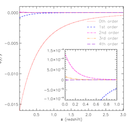
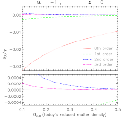
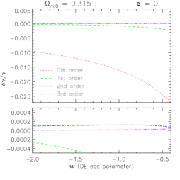
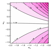
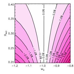
For , the relative error at order 1, at order 2 and at order 3. More generally, Figure 1 (upper right panel) shows that the accuracy of the approximation increases by roughly a factor of 10 as soon as a new coefficient is switched on. This same figure (lower right panel) shows that the relative accuracy depends only slightly on the equation of state parameter , although the error is in general slightly larger for larger . The relative error of the approximation is also quite stable as we vary within a sensitive range of values (see the lower left panel in Figure 1).
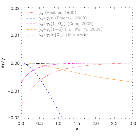
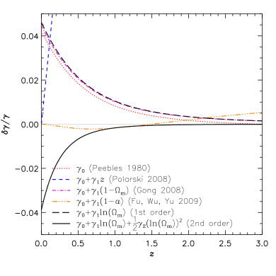
We remark that the coefficients and are the same111up to the sign of when expanding the growth index in powers of whereas and higher orders differ. However, as a consequence of developing in , already at first order our approximation is, depending on cosmology, from 5 to 10 times better at . This is seen in Figure 2, where we also compare the accuracy of Eq. (23) with various other parameterizations of the growth index. Not only Eq. (6) is more precise than formulas based on perturbative expansions around , in the relevant redshift range for dark energy studies, that is , it is also more accurate than the phenomenological [53] or perturbative [54] expressions normalized at .
3.1.2 Varying equation of state
We first compute the coefficients (see Eq. 20). If we assume , then the limit is equivalent to the limit . We obtain
| (25) |
etc., where from equation (18). The formalism requires the knowledge of the order derivative of the DE EoS for , that is well beyond the redshift domain where the expansion rate of the universe is expected to be sensitive to contributions from the dark energy density. Noting that when , the finiteness of the coefficients (at least up to ) can be enforced by requiring the EoS to satisfy the following equation
| (26) |
whose most general solution is
| (27) |
where , . Note that by linearizing the previous expression around one recovers the standard parameterization [71]. For this specific equation of state, we have
| (28) |
and, as a consequence, the coefficients of the series expansion which defines the growth index are
| (29a) | ||||
| (29b) | ||||
| (29c) | ||||
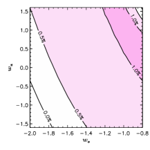
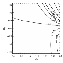
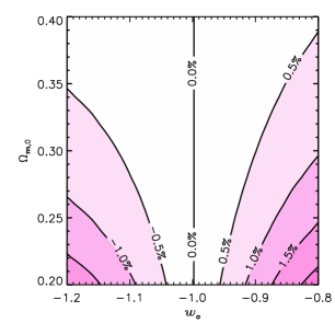
The relative variation of the growth index with respect to the CDM value, when the EoS parameters span the range () can be as large as at . As a reference, if is fixed to the value , then one can expect a relative difference as important as , a figure larger than the nominal precision with which a Euclid-like survey is expected to constrain , that is [47]. Figure 3 shows that within the redshift range that will be surveyed by Euclid (), already when truncating the expansion at first order, the maximal imprecision with which the redshift scaling of is reconstructed over all the parameter space is less than 0.1%.
We are not aware of any theoretically justified model that accounts for possible variability in the DE EoS, so we compare the accuracy of our parameterization (cf. Eqs. (29)) with that obtained using the Wang & Steinhardt (1998) model[49], which is supposed to be an accurate approximation also for weakly varying dark energy equation of states. Additionally, we also consider the phenomenological fitting formula of [50], (, where is the Heaviside step function and is the constant equation of state (EoS) parameter of the dark energy fluid). As can be appreciated by inspecting Figure 3, the gain in precision with respect to both these growth index models can be as high as 1 order of magnitude in the range (), a figure which pushes the systematic error well below the expected measurement precision of the Euclid satellite.
3.2 Clustering Dark Energy
Dark energy affects the process of structure formation not only through its equation of state, but also through its speed of sound. Indeed, if the speed of sound with which dark energy perturbations propagate drops below the speed of light, then dark energy inhomogeneities increase and couple gravitationally to matter perturbations. As a consequence, they may be detectable on correspondingly better observable (though typically still large) scales. The influence of an unstable dark energy component on the clustering of matter can be effectively described by switching on the additional degrees of freedom and in Eq. (2).
As an archetype of this class of phenomena, we consider the clustering dark energy model with vanishing speed of sound introduced in [74]. In this model, the dark energy EoS is assumed to be constant, the speed of sound is effectively null, and we have
| (30) |
As a consequence, the structural parameters of our formalism are
| (31a) | ||||||
| (31b) | ||||||
while and are the same as in Eq. (22). Using Eq. (9), it follows immediately that the growth index coefficients are
| (32a) | ||||
| (32b) | ||||
| (32c) | ||||
Note that, as for smooth quintessence, the CDM model is also included in clustering quintessence as the limiting case (as a matter of fact, by setting in Eqs. (32) we finde the coefficients (24)).
In Figure 4 we compare the exact numerical calculation of the growth index and the approximation (6) with coefficients and computed above. The relative discrepancy, for the characteristic values of and is shown in Figure 4. By comparing our parameterization of the growth index with that of Sefusatti and Vernizzi (2011) (left panel of Figure 4), we can appreciate the gain in precision, which is roughly a factor of 2.
4 Modified Gravity
In this section we show how to predict the amplitude of the growth index in scenarios where the Einstein fields equations are modified. We will first discuss what has become a reference benchmark for alternative gravitational scenarios, the DGP model [23], and we will then generalize the discussion, by applying the formalism to Post Parametrized Friedmann models [56].
4.1 The growth index as a diagnostic for the DGP model
We consider the Dvali-Gabadadze-Porrati brainworld model[23] in which gravity is modified at large distances due to an extra spatial dimension. The scale factor of the resulting cosmological model evolves according to the following modified Friedmann equation [24]
| (33) |
where is the length scale at which gravity starts to leak out into the bulk. Neglecting effects of spatial curvature () and defining , the Hubble rate can be expressed as
| (34) |
which implies the constraint . By deriving Eq. (33) with respect to and by using the standard energy conservation equation , we find, in terms of the fundamental variable of our formalism ()
| (35) |
from which it follows that the flat DGP model is formally equivalent to a DE model with an varying as . The effective Newton constant in the Poisson equation is [73, 64, 63]
| (36) |
and, after some algebra, the source term in Eq. (2) can be expressed as
| (37) |
From Eqs. (35), (37) and (7) we find the following structural parameters
| (38a) | ||||
| (38b) | ||||
and, finally, the growth index coefficients
| (39) |
In what follows we consider the flat DGP model with . With this choice of the density parameter, the DGP model best fits the expansion rate of the reference CDM model in the range . In this non-standard gravity scenario, the maximal relative error, when comparing the parametric reconstruction of the growth rate with numerical results in the redshift range covered by Euclid-like survey, is at order 1, and at order 2, see Fig 5. To sub percentage precision we need to expand the growth index one order further. The somewhat degraded precision for the DGP model is due to the fact that the Taylor parameterization proposed in this work (cf. the approximation (6)) is specifically tailored for models in which the growth index minimally deviates from the CDM prediction. It is however impressive how the DGP model, despite its extreme nature, can still be satisfactorily described by our formalism.
4.2 The growth index in general models of modified gravity
We will now assume that, in viable theories of modified gravity, both background and perturbed observables have values close to that of the standard cosmological model. That is, deviations from CDM are hypothesized to be small, comparable with current observational uncertainties. We further assume that Eq. (2) is the master equation for studying matter collapse on sub-horizon size. In other terms, linear density fluctuations evolve in the quasi-static Newtonian regime. This being the case, the structure coefficients of the growth index formalism are given by Eq. (7) and, by a straightforward implementation of formula (9), we obtain
| (40a) | |||||
| (40b) | |||||
| (40c) | |||||
One can parameterize a large class of modified gravity scenarios by expanding the model dependent quantities and in power series. Since we are interested in alternative gravitational scenarios that might explain away the dark energy phenomenon, we expect deviations from Einstein’s gravity to become appreciable as starts to diverge from 0. By assuming both and analytic at , we can thus expand (see also [56])
| (41a) | |||||
| (41b) | |||||
| (41c) | |||||
where we denoted by the value of the in the epoch of matter domination as in §3.1.2. The corresponding growth index coefficients are
| (42a) | |||||
| (42b) | |||||
| (42c) | |||||
4.2.1 The CDM framework
As an example of the application of the formalism, we consider the CDM scenario of [56]. This is a one-parameter family of models representing a large class of modified gravity theories for which the fundamental geometric degree of freedom is the metric, the field equations are at most 2nd order in the metric variables and gauge-invariant [75]. The interesting facet of these non-standard gravity models is that deviations from GR are parameterized by an observable, the gravitational slip parameter
| (43) |
where and are the Newton and curvature potentials respectively, both assumed to be time and scale dependent functions.
In this non-standard gravity formalism, the background evolution is degenerate with that of the CDM model of cosmology, that is it is effectively described by the Friedmann equation ((15)) augmented by a Dark Energy component with equation of state parameter , satisfying the usual conservation equation (13). This fixes the amplitude of the structural parameters of our formalism to those of (21).
Deviations from General Relativity are expected only in the perturbed sector of the theory. At first order, indeed, this class of models predicts the following modification of the Newton constant
| (44) |
where it is assumed that on small cosmic scales, well inside the horizon, any scale dependence in the gravitational slip parameter can be neglected. This in turns implies that the growth of matter perturbations, in these scenarios, can be described by inserting and into Eq. 3. Since, at early epochs deviations from General Relativity are constrained by Big Bang Nucleosynthesis measurements, it is a fair hypothesis to assume that is a smooth function which deviates from zero as soon as the dark energy comes to dominate the overall energy budget of the universe. As a result, the gravitational slip parameter can be expanded as [56]
| (45) |
and the overall effects of non-standard gravity are governed by the set of discrete parameters . From Eqs. (41) and (42) it is now easy to read off the value of the growth indices in the CDM model:
| (46a) | |||||
| (46b) | |||||
| (46c) | |||||
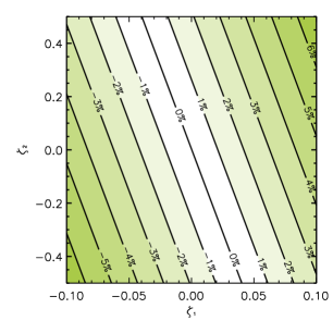
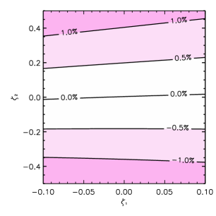
The amplitude of the non-standard signals expected in this alternative gravitational scenario is shown in the left panel of Figure 6 where we display the distortions which a possibly non-null value of the CDM parameters and induce on the growth index. Also the accuracy with which the growth index is reconstructed by our formalism is shown (left panel). This last plot confirms that systematic uncertainties are below the threshold of the Planck statistical errors over a region of the parameter space (, ) which is sufficiently large to be physically interesting.
| Label | Reference | ||
|---|---|---|---|
| THF | Turnbull et al. (2012) [34] | 0.02 | |
| DNM | Davis et al. (2011) [35] | 0.02 | |
| 6dFGS | Beutler et al. (2012) [36] | 0.07 | |
| 2dFGRS | Percival et al. (2004) [37], Song & Percival (2009) [38] | 0.17 | |
| 2SLAQ | Ross et al. (2007) [39] | 0.55 | |
| SDSS | Cabré et al. (2009) [40] | 0.34 | |
| SDSS II | Samushia et al. (2012) [41] | 0.25 | |
| 0.37 | |||
| BOSS | Reid et al. (2012) [42] | 0.57 | |
| WiggleZ | Contreras et al. (2013) [43] | 0.20 | |
| 0.40 | |||
| 0.60 | |||
| 0.76 | |||
| VVDS | Guzzo et al. (2008) [44], Song & Percival (2009) [38] | 0.77 | |
| VIPERS | De la Torre et al. (2013) [45] | 0.80 |
5 Data analysis in the growth index parameter space
Besides being instrumental in increasing the accuracy with which the growth rate is reconstructed from data, the -formalism introduced in the previous sections also serves as a guide in interpreting empirical results directly in terms of dark energy models. This is shown in this section, where we confront the growth index predictions with current data and data simulations for a Euclid-like survey. After describing our data analysis strategy, we show here how we test whether the CDM model correctly describes available data about the linear growth rate of structures and how we use the growth index parameter space to analyze and draw statistical conclusions on various non-standard gravity scenarios, in a manner which is independent from the specific details of the expansion history of the universe.
5.1 Testing the CDM predictions in the perturbed sector
We first focus on the constraints that present day observations set on the growth indices . These are derived by computing the likelihood of the data shown in Table 1 given the model in Eqs. (4) and (6). To this purpose we minimize the function
| (47) |
where is the uncertainty in the growth data, is the set of parameters that, except for , fix the background expansion, are the growth indices introduced in Eq. (6) and
| (48) | ||||
| (49) |
where is the growth factor. In this paper we restrict our analysis to the first two growth indices, i.e. we set . We also assume the measurements in Table 1 to be independent. A more sophisticated error analysis might eventually results in minor changes in our quantitative conclusions, but will have no impact on their physical interpretation. It is well known that cannot be estimated from data without picking a particular model, or at least a parametrization, for gravity, i.e., for the quantity being tested [72]. Despite the strong prior on the underlaying gravitational model, there is however evidence that the estimated values of this observable depend negligibly on the distance-redshift conversion model, that is for sensible variations of the background parameter in a flat CDM model, the variation of the estimation is well below the statistical error [45, 43]. This should guarantee that data can be meaningfully compared against models with distinct background evolution from that assumed to estimate the observable.
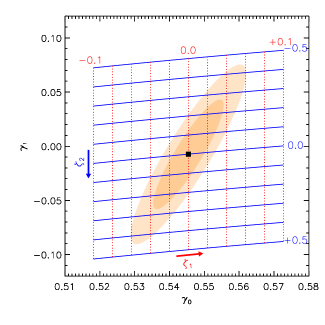
The likelihood analysis is carried out by choosing a prior model (hereafter called fiducial) for the evolution of and in Eqs. (49). To this purpose we choose the reference CDM model i.e. a flat CDM model with parameters [7]. The resulting likelihood contours for and are shown in the left panel of Figure 7. By marginalizing in the growth index parameter space we find that, at confidence level (c.l.), the relative precision on the leading and first order growth indices is and . On the right panel of Figure 7 we show the same analysis assuming WMAP9 background values . In this case, the 1-dimensional marginalized confidence levels are and . The likelihood contours are appreciably smaller if the likelihood analysis is carried out in the WMAP9 fiducial, owing to the fact that the statistical analysis depends on the background model. We will see in the next section how to factor out the specific choice of the background model from the interpretation of growth rate data.
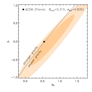
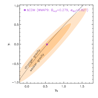
The traditional way of exploiting the growth index formalism is to use it as a tool for a consistency test of the scenario proposed to model the background kinematics of the universe. The goal is to check whether a given gravitational model that explains the observed cosmic expansion rate also predicts the correct growth rate of linear structures. For example, one needs to verify that the most likely amplitude of the growth index parameters derived from observations of the linear growth of structures is not in conflict with those predicted on the basis of the DE EoS parameters and which best fit expansion rate data. In absence of major observational systematics, any possible mismatch between measured and expected values of the growth index, would be the smoking gun of new gravitational physics. In the opposite case, growth data provide additional constraints on dark energy parameters.
Figure 7 shows that the growth index predicted on the basis of and , i.e. the EoS values of the reference CDM model agrees with results from the likelihood analysis of linear growth rate data coming from a variety of low redshift surveys of the large scale structure of the universe. Shouldn’t this be the case, one could question either the unbiased nature of the data analysis in both sectors, background and perturbed, either the effectiveness of the standard description of gravity in terms of a CDM framework.
A first immediate advantage of interpreting growth history data in the growth index plane, is that this parameter space facilitates the interpretation of critical information encoded in the likelihood function. Specifically, it allows to classify alternative dark energy models (each labeled by the pair of coordinates ) as either generating more or less growth of structures with respect to the chosen fiducial. The line separating these two characteristic regions is shown in Figure 7 and it is computed by imposing
| (50) |
where are the growth indices of the fiducial model (that is in Fig 7), are the background parameters of the fiducial model and is the initial redshift at which perturbations are conventionally assumed start growing. The region of more growth in the -plane is defined as the region where a density perturbation (whose amplitude is normalized to unity today) had, at the initial redshift, a smaller amplitude than that predicted in the fiducial model () whereas regions of weaker gravity are the loci where the amplitude of the perturbation was larger (). Note that the orientation of the line separating these two regions depends only negligibly on the chosen initial redshift (for the sake of illustration we have set in Figure 7). Our analysis shows that current data mildly favor models in which the strength of gravitational interactions is weaker than what is predicted in the reference CDM model. This result also confirms a conclusion of [46]. As compared to the way perturbations grow within purely matter-dominated models, it seems that data tend to prefer a suppression mechanism more efficient than that provided by the cosmological constant.
5.2 Discriminating DE models in the and parameter space
Once a fiducial for the background evolution is chosen to compute the likelihood function, what conclusions can we draw on the viability of gravitational models other than the fiducial itself? We will now see that, since the dependence of the growth index on the relevant cosmological parameters is explicitly taken into account in our analysis scheme, the likelihood in the plane, besides allowing to reject the null hypothesis that the fiducial is compatible with data, also allows to set constraints on alternative cosmological scenarios. In other terms, it is possible to exploit model dependent likelihood contours in the plane to tell apart also those theoretical models characterized by an evolution of the background sector which is distinct from that of the fiducial model itself.
The growth indices and are model dependent quantities which can be estimated only once a specific background fiducial model for the evolution of is chosen (cf. Eq. 48). As a consequence, the growth indices inferred in distinct background models cannot be directly compared. For example, consider the likelihood contours in the plane obtained by assuming the reference CDM model as fiducial (Figure 7). One cannot constrain the DE parameters and by simply computing the amplitude of the coefficients and expected in an effective DE model with parameters and (cf. §3.1.2) and by confronting these theoretical values with the empirical likelihood. Indeed, the specific growth rate history of a DE model is not entirely captured by the growth indices, part of the information being locked in the scaling of the background density parameter .
We overcome this critical pitfall by computing , the amplitude of the effective growth indices in the fiducial background, that is the exponent that once inserted in (4) together with the matter density parameter of the fiducial model adopted in the likelihood analysis (), allows to match the scaling of the growth rate expected in the specific gravitational model under consideration. This is equivalent to enforcing the following identity
| (51) |
By means of this transformation strategy we factor out the effect of expansion from the analysis of growth rate histories. We will illustrate this feature by simulating the constraints that the growth index parameters expected from a next generation survey such as the space mission Euclid will put on the background dark energy parameters and .
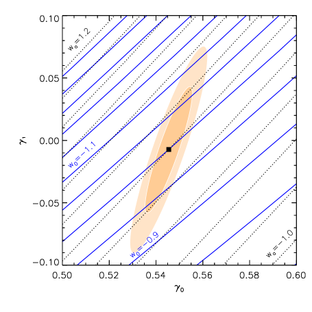
The Euclid mission is designed to survey, in spectroscopic mode, galaxies in the redshift range and in a sky area of deg2 [47]. We simulate the expected growth data assuming as fiducial, the reference CDM model. To this purpose, we simply split the redshift range into 14 intervals, and we predict by using Eqs. (19), (18) and (5). We finally assume that the relative error on the observable, in each interval, is that corresponding to the Euclid figure of merit listed in table 2.2 of [47], i.e. . The resulting likelihood contours in the plane, obtained via a standard analysis, are shown in Figure 8. Notice that the growth index figure of merit, defined as the inverse of the surface of the likelihood contour in the plane, is expected to increase by a factor when compared to that deduced from current constraints (see Figure 7).
In Figure 8 we also show the effective growth indices ( predicted by various DE models (labeled by the parameters and ) obtained by means of the transformation law (51). In practice we compute these effective growth indices () by minimizing numerically the integral
| (52) |
over the redshift range covered by observational data (i.e. for current data and for Euclid-data simulations). We have verified that this mapping is sufficiently precise over all the redshift intervals where acceleration effects are observable. For typical errors of order arise for the most extreme values of and shown in Figure 8. Therefore, this error is largely negligible with respect to the precision of the constraints. Note that while varying and , we have kept fixed , that is we overlook any possible degeneracy between the DE and matter density parameters entering the expansion rate . This essentially because the relative variation induced in the distance modulus by this simplifying assumption is less than in the domain of interest. Overall, Figure 8 shows how measurements in the perturbed sector help to tighten the constraints on background cosmological parameters, and, ultimately to discriminate among DE models. Specifically, we predict that growth rate data will provide independent constraints on the value of characterized by a relative(/absolute) precision of .
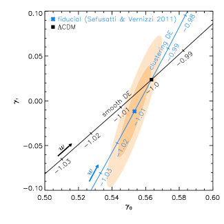
The remapping method illustrated by Eq. (51) provides a technique with which to tell apart gravitational models with identical background evolutions. In other terms we can use the growth index parameter space to resolve the background degeneracy of two dark energy models, i.e. two models predicting the same background expansions, but different linear growth histories. To illustrate this feature, we consider two possible scenarios whose background evolutions are degenerate with that of the CDM model: the clustering quintessence and the CDM models.
We first consider the case in which future Euclid data are simulated in a clustering quintessence model, a cosmological model in which matter is supplemented by a quintessence component with null sound speed, i.e. the model of [74] discussed in §3.2. Specifically, we forecast by using Eqs. (30), (18) and(5) and by further imposing that the background expansion is effectively described in terms of the constant DE EoS parameter . The likelihood contours in the plane, obtained by adopting as fiducial model the same clustering quintessence model used to simulate data, are displayed on the left panel of Figure 9. We now show how to use these measurements in the plane to tell apart the clustering quintessence from canonical smooth quintessence. To this purpose we calculate the effective growth indices and in two different theoretical models of dark energy, the clustering quintessence and the smooth quintessence models (both identified, for simplicity, via their constant parameter ). They are calculated by using Eq. (51) to map of Eqs. (29) and (32) respectively into the effective values for the fiducial background used to analyze growth data. By comparing likelihood results vs. the predicted amplitude of the growth index, we can appreciate how the smooth DE model with the same background expansion as the true cosmological model (in this context, the clustering quintessence model) is clearly ruled out at 95% c.l. by growth rate data. Specifically, if the effective EoS deviates from the reference value by at least ( or ) a Euclid-like survey has enough resolving power to discriminate between smooth and clustering quintessence.
As an additional example, on the right panel of Figure 9 we show the constraints that an Euclid-like survey can set on the slip parameter entering the CDM model reviewed in §4.2.1. To this purpose we simulate Euclid observations assuming the reference CDM model and we then reconstruct the likelihood assuming this very same model as fiducial. We then compare this statistic to prediction from the CDM model, that is to the values and of Eqs. (46) computed for different values of the slip parameters and defined in equation (45) (for simplicity we here explore only models for which and ). Note that, in this particular case, owing to the fact that the background evolution does not change from model to model, the remapping procedure is superfluous. The right panel of Figure 9 displays the performances of an Euclid-like survey in detecting possible deviations of the slip parameter from its GR value, i.e from zero. We can conclude that data will have enough resolving power to exclude, at the 95% c.l., models predicting a parameter larger than 0.025 , or in other terms data can detect a relative deviation between the Newtonian and the curvature potential if it is larger than about 2.5%.
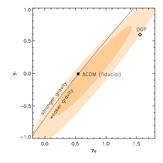

Up to this point, we have shown that models with distinct background evolutions and models with distinct growth rate predictions can be analyzed in the same parameter space, thanks to the remapping scheme of Eq. (51). A neat way to demonstrate the precision and consistency of this strategy is by showing that the conclusions on the physical viability of a model are invariant with respect to the choice of the fiducial in which data are analyzed. We will demonstrate this key feature by exploiting the DGP[23] model which predicts both different background and different growth rate evolutions with respect to the CDM model. To this purpose, as in §4.1 we consider the flat DGP model which best fits the expansion rate of the reference CDM model. This DGP model has parameters , where the effective DGP is given in §4.1.
In Figure 10 we show the constraints set on the DGP model by current data (cf. Table 1). In the left panel, we show the likelihood contours in the parameter plane obtained by using as fiducial for the evolution of the background metric the expansion rate of the reference CDM model. The prediction for the DGP model obtained with the mapping (51) is also shown. In the right panel, instead, we show the likelihood contours in the parameter plane obtained by using the expansion rate of the DGP model as fiducial for the evolution of the background metric. In this case, it is the predictions of the CDM model that are remapped via Eq. (51). By confronting these two plots we see that while the location, the amplitude and the orientation of the likelihood surfaces do vary, the interpretation of the results is clearly unchanged. Both figures show, consistently, that measurements of the growth rate in the range have already a sufficient precision to rule out, at a c.l., a most extreme scenario of modified gravity such as the DGP model. In other terms, the structure of the likelihood contours depends on the specific fiducial model of the background, that is each fiducial background defines its own growth index parameter space. But physical interpretation is unchanged if we change from one parameter space to the other using the transformation equation (51).
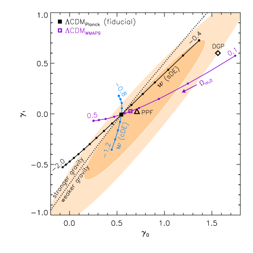
The advantage of the method is also illustrated in Figure 11 using current data. In this picture we simultaneously contrast predictions from a large class of cosmological models against the likelihood contours derived assuming the reference CDM as fiducial for data analysis. On top of the DGP model (black diamond), we also plot the effective growth indices associated to the CDM model which best fits WMAP9 data [6] (purple empty square). In this scenario, characterized by the reduced density parameter , the growth of structures is slightly suppressed with respect to the fiducial, i.e. the reference CDM model of Planck. One might also remark the slight (but statistically insignificant) tendency of growth data to favor the WMAP9 substantiation of the CDM model with respect to the Planck one. This is a particular example of a general feature of CDM models: the higher the matter density and the more severe the tension with growth index constraints. For example CDM models with are excluded at confidence level. In Figure 11 we also show the constraints on DE models with constant parameter . Smooth DE models with and Clustering DE models with are excluded at confidence level. Finally, as a curiosity, we show that a CDM model (black empty triangle) with the same background as the reference CDM model but with a slip parameter best fits observations, that is it maximizes the likelihood of current data.
6 Conclusions
The observational information about the growth rate history of linear cosmic structures can be satisfactorily encoded into a small set of parameters, the growth indices , whose amplitude can be analytically predicted by theory. Their measurement allows to explore whether Einstein’s field equations encompass gravity also in the infrared, i.e. on very large cosmic scales. In order for this to be accomplished, a) an optimal scheme for compressing the growth rate function into the smallest possible set of discrete scalars , without sacrifying accuracy, and b) a prescription for routinely calculating their amplitude in relevant theories of gravity, in order to explore the largest region in the space of all possible models, must be devised.
In this paper we have explored a promising approach towards this goal. We have demonstrated both the precision and the flexibility of a specific parameterization of the growth index, that is the logarithmic expansion (6). If the fiducial gravitational model is not too different from standard GR, i.e. possible deviations in both the background and perturbed sector can be interpreted as first order correction to the Friedmann model, then the proposed parameterization scheme allows to match numerical results on the redshift dependence of the growth index with a relative error which is lower than the nominal precision with which the next generation of redshift surveys are expected to fix the scaling of this function. The performances are demonstrated by comparing, for various fiducial gravitational models, the accuracy of our proposal against that of different parameterizations available in the literature.
Besides accuracy, the formalism features two other critical merits, one practical and one conceptual. First we supply a simple way for routinely calculating the amplitude of the growth indices in any gravitational model in which the master equation for the growth of density perturbations reduces to the form of Eq. 2. To this purpose it is enough to specify three characteristic functions of this equation, the expansion rate , the damping and the response coefficients to calculate the parameters up to any desired order . Moreover, since the parameterization of the growth rate has not a phenomenological nature, but it is constructed as a series expansion of the exact solutions of the differential equation which rules the growth of structures (cf. Eq. 3), one can easily interpret empirical results about the amplitude of the growth indices in terms of fundamental gravitational models.
Since the growth index is a model dependent quantity, it has been traditionally used only to reject, statistically, the specific model adopted to analyze growth data. We have shown, instead, that the growth index parameter space provides a diagnostic tool to discriminate a large class of models, even those presenting background evolution histories different from the fiducial model adopted in data analysis. In other terms, a detection of a present day growth index amplitude would not only indicate a deviation from CDM predictions but could be used to disentangle among different alternative explanations of the cosmic acceleration in a straightforward way. The key to this feature is the mapping of Eq. 51 which allows to factor out the effect of expansion from the analysis of growth rate histories. As the standard plane identifies different expansion histories , the plane can thus be used to locate different growth rate histories .
We have illustrated the performance of the growth index plane in relation to modify gravity model selection/exclusion by using current data as well as forecasts from future experiments. We have shown that the likelihood contours in the growth index plane can be used to tell apart a clustering quintessence component [74] from a smooth dark energy fluid, to fix the parameters of viable Parameterized Post Friedman gravitational models [56] or to exclude specific gravitational models such as, for example, DGP [23].
The performances of the analysis tool presented in this paper are expected to be enhanced, should the formalism be coupled to models parameterizing the large class of possible gravitational alternatives to standard GR available in the literature. In particular various approaches have been proposed to synthetically describe all the possible gravitational laws generated by adding a single scalar degree of freedom to Einstein’s equations [30, 31, 32, 76]. Besides quintessence, scalar-tensor theory and gravity, this formalism allows also to describe covariant Galileons [77], kinetic gravity braiding [78] and Horndeski/generalized Galileons theories [79, 80]. Interestingly, the cosmological perturbation theory of this general class of models can be parameterized so that a direct correspondence between the parameterization and the underlying space of theories is maintained. In a different paper [69] we have already explored how the effective field theory formalism of [30] allows to interpret the empirical constraints on directly in terms of fundamental gravity theories.
Acknowledgments
We acknowledge useful discussions with L. Guzzo, F. Piazza, T. Schücker, P. Taxil and J. M. Virey. CM is grateful for support from specific project funding of the Institut Universitaire de France and of the Labex OCEVU.
References
- [1] S. Perlmutter et al. (SNCP Collaboration), ”Measurements of and from 42 High-Redshift Supernovae”, ApJ 517, 565 (1999) [astro-ph/9812133]
- [2] A. G. Riess et al. (SNST Collaboration), ”Observational Evidence from Supernovae for an Accelerating Universe and a Cosmological Constant”, AJ 116, 1009 (1998) [astro-ph/9805201]
- [3] P. Astier et al. (SNLS Collaboration), ”The Supernova Legacy Survey: Measurement of , and from the First Year Data Set”, A&A 447, 31 (2006) [astro-ph/0510447]
- [4] C. Marinoni and A. Buzzi, ”A geometric measure of dark energy with pairs of galaxies”, Nature 468, 539 (2010)
- [5] E. Komatsu et al. (WMAP Collaboration), ”Seven-Year Wilkinson Microwave Anisotropy Probe (WMAP) Observations: Cosmological Interpretation”, ApJS 192, 18 (2011) [arXiv:1001.4538]
- [6] G. Hinshaw et al. (WMAP Collaboration), ”Nine-Year Wilkinson Microwave Anisotropy Probe (WMAP) Observations: Cosmological Parameter Results”, ApJS 208, 19 (2013) [arXiv:1212.5226]
- [7] P. A. R. Ade et al. ( Collaboration), ”Planck 2013 results. XVI. Cosmological parameters”, [arXiv:1303.5076]
- [8] L. Anderson, E. Aubourg, S. Bailey, et al., ”The clustering of galaxies in the SDSS-III Baryon Oscillation Spectroscopic Survey: Baryon Acoustic Oscillations in the Data Release 9 Spectroscopic Galaxy Sample”, MNRAS 427, 3435 (2013) [arXiv:1203.6594]
- [9] J. Bel, C. Marinoni, B. R. Granett, L. Guzzo, J. A. Peacock, E. Branchini et al., ”The VIMOS Public Extragalactic Redshift Survey (VIPERS): from the galaxy clustering ratio measured at ”, A&A 563, A37 (2014) [arXiv:1310.3380]
- [10] A. G. Sanchez, C. G. Scóccola, A. J. Ross et al., ”The clustering of galaxies in the SDSS-III Baryon Oscillation Spectroscopic Survey: cosmological implications of the large-scale two-point correlation function”, MNRAS 425, 415 (2012) [arXiv:1203.6616]
- [11] P. J. E. Peebles and B. Ratra, ”The Cosmological constant and dark energy”, Rev. Mod. Phys. 75, 559 (2003) [astro-ph/0207347]
- [12] L. Amendola and S. Tsujikawa, ”Dark Energy: Theory and Observations”, Cambridge U. P. (2011)
- [13] E. J. Copeland, M. Sami and S. Tsujikawa, ”Dynamics of dark energy”, Int. J. Mod. Phys. D 15, 1753 (2006) [hep-th/0603057]
- [14] C. Wetterich, ”Cosmology and the Fate of Dilatation Symmetry”, Nucl. Phys. B 302 668 (1988)
- [15] R. R. Caldwell, R. Dave and P. J. Steinhardt, ”Cosmological imprint of an energy component with general equation of state”, Phys. Rev. Lett. 80 , 1582 (1998) [astro-ph/9708069]
- [16] C. Armendariz-Picon, V. F. Mukhanov and P. J. Steinhardt, ”A Dynamical Solution to the Problem of a Small Cosmological Constant and Late-time Cosmic Acceleration”, Phys. Rev. Lett. 85, 4438 (2000) [astro-ph/0004134]
- [17] P. Binetruy, ”Cosmological constant versus quintessence”, Int. J. Theor. Phys. 39, 1859 (2000) [hep-ph/0005037]
- [18] J. P. Uzan, ”Cosmological scaling solutions of nonminimally coupled scalar fields”, Phys. Rev. D 59 (1999) 123510 [gr-qc/9903004]
- [19] A. Riazuelo and J. P. Uzan, ”Cosmological observations in scalar - tensor quintessence”, Phys. Rev. D 66 023525 (2002) [astro-ph/0107386]
- [20] M. Gasperini, F. Piazza and G. Veneziano, ”Quintessence as a runaway dilaton”, Phys. Rev. D 65, 023508 (2002) [gr-qc/0108016]
- [21] T. Clifton, P. G. Ferreira, A. Padilla and C. Skordis, ”Modified Gravity and Cosmology”, Phys. Rept. 513, 1 (2012) [arXiv:1106.2476]
- [22] A. De Felice and S. Tsujikawa, ” theories”, Living Rev. Rel. 13, 3 (2010) [arXiv:1002.4928]
- [23] G. R. Dvali, G. Gabadadze, and M. Porrati, ”4-D gravity on a brane in 5-D Minkowski space”, Phys. Lett. B. 485, 208 (2000) [hep-th/0005016]
- [24] C. Deffayet, G. R. Dvali and G. Gabadadze, ”Accelerated universe from gravity leaking to extra dimensions”, Phys. Rev. D 65, 044023 (2002) [astro-ph/0105068]
- [25] N. Arkani-Hamed, S. Dimopoulos, G. Dvali and G. Gabadadze, ”Nonlocal modification of gravity and the cosmological constant problem” [arXiv:hep-th/0209227]
- [26] S. Capozziello, S. Carloni and A. Troisi, ”Quintessence without scalar fields”, Recent Res. Dev. Astron. Astrophys. 1, 625 (2003) [arXiv:astro-ph/0303041]
- [27] S. ’i. Nojiri and S. D. Odintsov, ”Modified Gauss-Bonnet theory as gravitational alternative for dark energy”, Phys. Lett. B 631, 1 (2005) [hep-th/0508049]
- [28] C. de Rham, G. Gabadadze and A. J. Tolley, ”Resummation of Massive Gravity”, Phys. Rev. Lett. 106, 231101 (2011) [arXiv:1011.1232]
- [29] F. Piazza, ”The IR-Completion of Gravity: What happens at Hubble Scales?”, New J. Phys. 11, 113050 (2009) [arXiv:0907.0765]
- [30] G. Gubitosi, F. Piazza and F. Vernizzi, ”The Effective Field Theory of Dark Energy”, JCAP 1302, 032 (2013) [arXiv:1210.0201]
- [31] J. Gleyzes, D. Langlois, F. Piazza and F. Vernizzi, ”Essential Building Blocks of Dark Energy”, JCAP 1308, 025 (2013) [arXiv:1304.4840]
- [32] T. Baker, P. G. Ferreira and C. Skordis, ”The Parameterized Post-Friedmann Framework for Theories of Modified Gravity: Concepts, Formalism and Examples”, Phys. Rev. D 87, 024015 (2013) [arXiv:1209.2117]
- [33] J. Bel and C. Marinoni, ”Determination of the abundance of cosmic matter via the cell count moments of the galaxy distribution”, A&A 563, A36 (2014) [arXiv:1210.2365]
- [34] S. J. Turnbull, M. J. Hudson, H. A. Feldman et al., ”Cosmic flows in the nearby universe from Type Ia Supernovae”, MNRAS 420, 447 (2012) [arXiv:1111.0631v2]
- [35] M. Davis, A. Nusser, K. L. Masters et al., ”Local Gravity versus Local Velocity: Solutions for and nonlinear bias”, MNRAS 413, 2906 (2011) [arXiv:1011.3114]
- [36] F. Beutler, C. Blake, M. Colless et al., ”The 6dF Galaxy Survey: measurement of the growth rate and ”, MNRAS 423, 3430 (2012) [arXiv:1204.4725]
- [37] W. J. Percival et al. (2dFGRS Coll.), ”The 2dF Galaxy Redshift Survey: Spherical harmonics analysis of fluctuations in the final catalogue”, MNRAS 353, 1201 (2004) [astro-ph/0406513]
- [38] Y.-S. Song and W. J. Percival, ”Reconstructing the history of structure formation using Redshift Distortions”, JCAP 10, 4 (2009) [arXiv:0807.0810]
- [39] N. P. Ross, J. da Ângela, T. Shanks et al., ”The 2dF-SDSS LRG and QSO Survey: The 2-Point Correlation Function and Redshift-Space Distortions”, MNRAS 381, 573 (2007) [astro-ph/0612400]
- [40] A. Cabré and E. Gaztañaga, ”Clustering of luminous red galaxies I: large scale redshift space distortions”, MNRAS 393, 1183 (2009) [arXiv:0807.2460]
- [41] L. Samushia, W. J. Percival, A. Raccanelli, ”Interpreting large-scale redshift-space distortion measurements”, MNRAS 420, 2102 (2012) [arXiv:1102.1014]
- [42] B. A. Reid, L. Samushia, M. White et al., ”The clustering of galaxies in the SDSS-III Baryon Oscillation Spectroscopic Survey: measurements of the growth of structure and expansion rate at from anisotropic clustering” [arXiv:1203.6641]
- [43] C. Contreras et al. (WiggleZ Collaboration), ”The WiggleZ Dark Energy Survey: measuring the cosmic growth rate with the two-point galaxy correlation function”, MNRAS Advance Access (2013) [arXiv:1302.5178]
- [44] L. Guzzo, M. Pierleoni, B. Meneux et al., ”A test of the nature of cosmic acceleration using galaxy redshift distortions”, Nature 451, 541 (2008) [arXiv:0802.1944]
- [45] S. de la Torre, L. Guzzo, J. Peacock et al., ”The VIMOS Public Extragalactic Redshift Survey (VIPERS). Galaxy clustering and redshift-space distortions at in the first data release” [arXiv:1303.2622]
- [46] L. Samushia, B. A. Reid, M. White et al., ”The Clustering of Galaxies in the SDSS-III Baryon Oscillation Spectroscopic Survey: Measuring growth rate and geometry with anisotropic clustering” [arxiv:1312.4899]
- [47] R. Laureijs et al. (EUCLID Consortium), ”Euclid Definition Study Report” [arXiv:1110.3193]
- [48] P. J. E. Peebles, ”The Large Scale Structure of the Universe”, Princeton University Press (1980)
- [49] L. Wang, P. J. Steinhardt, ”Cluster abundance constraints on quintessence models”, ApJ 508, 483 (1998) [astro-ph/9804015]
- [50] E. V. Linder, ”Cosmic growth history and expansion history”, Phys. Rev. D 72, 043529 (2005) [astro-ph/0507263]
- [51] Y. Gong, ”The growth factor parameterization and modified gravity”, Phys. Rev. D 78, 123010 (2008) [arXiv:0808.1316]
- [52] R. Gannouji, B. Moraes, and D. Polarski, ”The growth of matter perturbations in models”, JCAP 0902, 034 (2009) [arXiv:0809.3374]
- [53] P. Wu, H. Yu, X. Fu, ”A Parametrization for the growth index of linear matter perturbations”, JCAP 0906, 019 (2009) [arXiv:0905.3444]
- [54] D. Polarski and R. Gannouji, ”On the growth of linear perturbations”, Phys. Lett. B 660, 439 (2008) [arXiv:0710.1510]
- [55] R. Gannouji and D. Polarski, ”The growth of matter perturbations in some scalar-tensor DE models”, JCAP 05, 018 (2008) [arXiv:0802.4196]
- [56] P. G. Ferreira, C. Skordis, ”The linear growth rate of structure in Parametrized Post Friedmannian Universes”, Phys. Rev. D 81, 104020 (2010) [arXiv:1003.4231]
- [57] M. Kunz, D. Sapone, ”Dark Energy versus Modified Gravity”, Phys. Rev. Lett. 98, 121301 (2007) [astro-ph/0612452]
- [58] V. Silvera and I. Waga, ”Decaying Lambda cosmologies and power spectrum”, Phys. Rev. D 50, 4890 (1994)
- [59] M. Sereno and J. A. Peacock, ”Imprints of deviations from the gravitational inverse-square law on the power spectrum of mass fluctuations”, MNRAS 371, 719 (2006) [astro-ph/0605498]
- [60] L. Knox, Y.-S. Song, and J. A. Tyson, ”Distance-redshift and growth-redshift relations as two windows on acceleration and gravitation: Dark energy or new gravity?”, Phys. Rev. D 74, 023512 (2006) [astro-ph/0503644]
- [61] M. Ishak, A. Upadhye, and D. N. Spergel, ”Probing cosmic acceleration beyond the equation of state: Distinguishing between dark energy and modified gravity models”, Phys. Rev. D 74, 043513 (2006) [astro-ph/0507184]
- [62] D. Sapone and L. Amendola, ”Constraining the growth factor with baryon oscillations” [arXiv:0709.2792]
- [63] S. Nesseris and L. Perivolaropoulos, ”Testing CDM with the Growth Function : Current Constraints”, Phys. Rev. D 77, 023504 (2008) [arXiv:0710.1092]
- [64] C. Di Porto and L. Amendola, ”Observational constraints on the linear fluctuation growth rate”, Phys. Rev. D 77, 083508 (2008) [arXiv:0707.2686]
- [65] A. Bueno Belloso, J. Garcia-Bellido and D. Sapone, ”A parametrization of the growth index of matter perturbations in various Dark Energy models and observational prospects using a Euclid-like survey” [arXiv:1105.4825]
- [66] C. Di Porto, L. Amendola and E. Branchini, ”Growth factor and galaxy bias from future redshift surveys: a study on parametrizations”, MNRAS 419, 985 (2012) [arXiv:1101.2453]
- [67] V. Cardone, S. Camera and A. Diaferio, ”An updated analysis of two classes of f(R) theories of gravity”, JCAP 1202, 030 (2012) [arXiv:1201.3272]
- [68] S. Basilakos and A. Pouri, ”The growth index of matter perturbations and modified gravity”, MNRAS 423, 3761 (2012) [arXiv:1203.6724]
- [69] F. Piazza, H. Steigerwald and C. Marinoni, ”Phenomenology of dark energy: exploring the space of theories with future redshift surveys” (2013) [arXiv:1312.6111]
- [70] P. Creminelli, G. D’Amico, J. Norena and F. Vernizzi, ”The Effective Theory of Quintessence: the Side Unveiled”, JCAP 0902, 018 (2009) [arXiv:0811.0827]
- [71] M. Chevallier and D. Polarski, ”Accelerating Universes with Scaling Dark Matter”, Int. J. Mod. Phys. D 10, 213 (2000) [arXiv:gr-qc/0009008]
- [72] M. Motta, I. Sawicki, I. D. Saltas, L. Amendola, and M. Kunz, ”Probing Dark Energy through Scale Dependence”, Phys. Rev. D 88, 124035 (2013) [arXiv:1305.0008]
- [73] A. Lue, ”The Phenomenology of Dvali-Gabadadze-Porrati Cosmologies”, Phys. Rept. 423, 1 (2006) [astro-ph/0510068]
- [74] E. Sefusatti and F. Vernizzi, ”Cosmological structure formation with clustering quintessence”, JCAP 1103, 047 (2011) [arXiv:1101.1026]
- [75] C. Skordis, ”Consistent cosmological modifications to the Einstein equations ”, Phys. Rev. D 79, 123527 (2009) [arXiv:0806.1238]
- [76] J. K. Bloomfield, E. E. Flanagan, M. Park and S. Watson, ”Dark energy or modified gravity? An effective field theory approach”, JCAP 08, 010 (2013) [arXiv:1211.7054]
- [77] A. Nicolis, R. Rattazzi and E. Trincherini, ”The Galileon as a local modification of gravity”, Phys. Rev. D 79, 064036 (2009) [arXiv:0811.2197]
- [78] C. Deffayet, O. Pujolas, I. Sawicki and A. Vikman, ”Imperfect Dark Energy from Kinetic Gravity Braiding”, JCAP 1010, 026 (2010) [arXiv:1008.0048]
- [79] G. W. Horndeski, ”Second-order scalar-tensor field equations in a four-dimensional space”, Int. J. Theor. Phys. 10, 363 (1974)
- [80] C. Deffayet, G. Esposito-Farèse and A. Vikman, ”Covariant Galileon”, Phys. Rev. D 79, 084003 (2009) [arXiv:0901.1314]
7 Appendix A: Amplitude of the growth indices
We compute the amplitude of the growth indices as follows. First we introduce Eq. (6) into Eq. (5) and obtain
| (53) |
Neglecting the term on the right hand side, we have transformed the first order non-linear differential equation (3) into an algebraic equation of the form
| (54) |
Now we set in Eq. (53) and we obtain
| (55) |
We suppose that , and in any viable model. In order to compute the coefficients up to an order , we have to expand as a Taylor series of at up to an order :
| (56) |
Eq. (54) is satified if and only if all the coefficients vanish:
| (57) |
This leads naturally to the definition of the structural coefficients (7). For in Eq. (57) we obtain Eq. (8). Finally, inverting Eq. (57) for leads to the recursion formula (9).