Decoding coalescent hidden Markov models in linear time

Kelley Harris1, Sara Sheehan2, John A. Kamm3, and Yun S. Song2,3,4

1Department of Mathematics, University of California, Berkeley

2Computer Science Division, University of California, Berkeley

3Department of Statistics, University of California, Berkeley

4Department of Integrative Biology, University of California, Berkeley

kharris@math.berkeley.edu, ssheehan@eecs.berkeley.edu, jkamm@stat.berkeley.edu, yss@eecs.berkeley.edu

Abstract

In many areas of computational biology, hidden Markov models (HMMs) have been used to model local genomic features. In particular, coalescent HMMs have been used to infer ancient population sizes, migration rates, divergence times, and other parameters such as mutation and recombination rates. As more loci, sequences, and hidden states are added to the model, however, the runtime of coalescent HMMs can quickly become prohibitive. Here we present a new algorithm for reducing the runtime of coalescent HMMs from quadratic in the number of hidden time states to linear, without making any additional approximations. Our algorithm can be incorporated into various coalescent HMMs, including the popular method PSMC for inferring variable effective population sizes. Here we implement this algorithm to speed up our demographic inference method diCal, which is equivalent to PSMC when applied to a sample of two haplotypes. We demonstrate that the linear-time method can reconstruct a population size change history more accurately than the quadratic-time method, given similar computation resources. We also apply the method to data from the 1000 Genomes project, inferring a high-resolution history of size changes in the European population.

To appear in the Proceedings of the 18th Annual International Conference on Research in Computational Molecular Biology (RECOMB 2014). The final publication is available at link.springer.com.

1 Introduction

The hidden Markov model (HMM) is a natural and powerful device for learning functional and evolutionary attributes of DNA sequence data. Given an emitted sequence of base pairs or amino acids, the HMM is well-suited to locating hidden features of interest such as genes and promotor regions [2, 5]. HMMs can also be used to infer hidden attributes of a collection of related DNA sequences. In this case, emitted states are a tuple of A’s, C’s, G’s and T’s, and the diversity of emitted states in a particular region can be used to infer the local evolutionary history of the sequences. When two sequences are identical throughout a long genetic region, they most likely inherited that region identical by descent from a recent common ancestor. Conversely, high genetic divergence indicates that the sequences diverged from a very ancient common ancestor [1, 15].

In recent years, coalescent HMMs such as the Pairwise Sequentially Markov Coalescent (PSMC) [15] have been used to infer the sequence of times to most recent common ancestor (TMRCAs) along a pair of homologous DNA sequences. Two other coalescent HMMs (CoalHMM [12, 4, 16] and diCal [24, 25]) also tackle the problem of inferring genealogical information in samples of more than two haplotypes. These methods are all derived from the coalescent with recombination, a stochastic process that encapsulates the history of a collection of DNA sequences as an ancestral recombination graph (ARG) [13, 29]. The hidden state associated with each genetic locus is a tree with time-weighted edges, and neighboring trees in the sequence are highly correlated with each other. Sequential changes in tree structure reflect the process of genetic recombination that slowly breaks up ancestral haplotypes over time.

The methods mentioned above all infer approximate ARGs for the purpose of demographic inference, either detecting historical changes in effective population size or estimating times of divergence and admixture between different populations or species. PSMC and CoalHMM have been used to infer ancestral population sizes in a variety of non-model organisms for which only a single genome is available [6, 19, 17, 30, 20, 28], as well as for the Neanderthal and Denisovan archaic hominid genomes [18]. Despite this progress, the demographic inference problem is far from solved, even for extremely well-studied species like Homo sapiens and Drosophila melanogaster [23, 7, 15, 27, 9]. Estimates of the population divergence time between European and African humans range from 50 to 120 thousand years ago (kya), while estimates of the speciation time between polar bears and brown bears range from 50 kya to 4 million years ago [10, 19, 3]. One reason that different demographic methods often infer conflicting histories is that they make different trade-offs between the mathematical precision of the model and scalability to larger input datasets. This is even true within the class of coalescent HMMs, which are much more similar to each other than to methods that infer demography from summary statistics [8, 21, 11] or Markov chain Monte Carlo [7].

Exact inference of the posterior distribution of ARGs given data is a very challenging problem, the major reason being that the space of hidden states is infinite, parameterized by continuous coalescence times. In practice, when a coalescent HMM is implemented, time needs to be discretized and confined to a finite range of values. It is a difficult problem to choose an optimal time discretization that balances the information content of a dataset, the complexity of the analysis, and the desire to infer particular periods of history at high resolution. Recent demographic history is often of particular interest, but large sample sizes are needed to distinguish between the population sizes at time points that are very close together or very close to the present.

In a coalescent HMM under a given demographic model, optimal demographic parameters can be inferred using an expectation-maximization (EM) algorithm. The speed of this EM algorithm is a function of at least three variables: the length L𝐿L of the genomic region being analyzed, the number n𝑛n of sampled haplotypes, and the number d𝑑d of states for discretized time. In most cases, the complexity is linear in L𝐿L, but the complexity in n𝑛n can be enormous because the number of distinct n𝑛n-leaved tree topologies grows super-exponentially with n𝑛n. PSMC and CoalHMM avoid this problem by restricting n𝑛n to be very small, analyzing no more than four haplotypes at a time. diCal admits larger values of n𝑛n by using a trunk genealogy approximation (see [22, 24, 25] for details) which is derived from the diffusion process dual to the coalescent process, sacrificing information about the exact structure of local genealogies in order to analyze large samples which are informative about the recent past.

To date, all published coalescent HMMs have had quadratic complexity in d𝑑d. This presents a significant limitation given that small values of d𝑑d lead to biased parameter estimates [16] and limit the power of the method to resolve complex demographic histories. PSMC is typically run with a discretization of size d=64𝑑64d=64, but diCal and CoalHMM analyses of larger datasets are restricted to coarser discretizations by the cost of increasing the sample size. In this paper, we exploit the natural symmetries of the coalescent process to derive an alternate EM algorithm with linear complexity in d𝑑d. The speedup requires no approximations to the usual forward-backward probabilities; we perform an exact computation of the likelihood in O(d)𝑂𝑑O(d) time rather than O(d2)𝑂superscript𝑑2O(d^{2}) time using an augmented HMM. We implement the algorithms presented in this paper to speed up our published method diCal, which is equivalent to PSMC when the sample size is two, yielding results of the same quality as earlier work in a fraction of the runtime. We have included the speedup in the most recent version of our program diCal; source code can be downloaded at http://sourceforge.net/projects/dical/.

2 Linear-Time Computation of the Forward and Backward Probabilities

We consider a coalescent HMM \mathcal{M} with hidden states S1,,SLsubscript𝑆1subscript𝑆𝐿S_{1},\ldots,S_{L} and observations x=x1,,xL𝑥subscript𝑥1subscript𝑥𝐿x=x_{1},\ldots,x_{L}. For PSMC, Ssubscript𝑆S_{\ell} is the discretized time interval in which two homologous chromosomes coalesce at locus \ell, while xsubscript𝑥x_{\ell} is an indicator for heterozygosity. The method diCal is based on the conditional sampling distribution (CSD) which describes the probability of observing a newly sampled haplotype x𝑥x given a collection \mathcal{H} of n𝑛n already observed haplotypes. In diCal, the hidden state at locus \ell is S=(H,T)subscript𝑆subscript𝐻subscript𝑇S_{\ell}=(H_{\ell},T_{\ell}), where Hsubscript𝐻H_{\ell}\in\mathcal{H} denotes the haplotype in the “trunk genealogy” (see [22]) with which x𝑥x coalesces at locus \ell and T{1,,d}subscript𝑇1𝑑T_{\ell}\in\{1,\ldots,d\} denotes the discretized time interval of coalescence; the observation x𝒜subscript𝑥𝒜x_{\ell}\in\mathcal{A} is the allele of haplotype x𝑥x at locus \ell. For n=||=1𝑛1n=|\mathcal{H}|=1, diCal is equivalent to PSMC. In what follows, we present our algorithm in the context of diCal, but we note that the same underlying idea can be applied to other coalescent HMMs.

2.1 A linear-time forward algorithm

We use f(x1:,(h,j))𝑓subscript𝑥:1𝑗f(x_{1:\ell},(h,j)) to denote the joint forward probability of observing the partial emitted sequence x1::=x1,,xassignsubscript𝑥:1subscript𝑥1subscript𝑥x_{1:\ell}:=x_{1},\ldots,x_{\ell} and the hidden state S=(h,j)subscript𝑆𝑗S_{\ell}=(h,j) at locus \ell. The probability of transitioning from state (h,k)superscript𝑘(h^{\prime},k) at locus \ell to state (h,j)𝑗(h,j) at locus +11\ell+1 is denoted by ϕ(h,jh,k)italic-ϕconditional𝑗superscript𝑘\phi(h,j\mid h^{\prime},k), the stationary probability of state (h,i)𝑖(h,i) is denoted ζ(h,i)𝜁𝑖\zeta(h,i), and the emission probability of the observed allele x=asubscript𝑥𝑎x_{\ell}=a given coalescence at T=jsubscript𝑇𝑗T_{\ell}=j onto haplotype hh with allele h=bsubscript𝑏h_{\ell}=b at locus \ell is denoted by ξ(ab,j)𝜉conditional𝑎𝑏𝑗\xi(a\mid b,j). When \ell is obvious from the context, we sometimes use ξ(as):=ξ(ah,j)assign𝜉conditional𝑎𝑠𝜉conditional𝑎subscript𝑗\xi(a\mid s):=\xi(a\mid h_{\ell},j) for s=(h,j)𝑠𝑗s=(h,j). Explicit expressions for ζ(h,i)𝜁𝑖\zeta(h,i), ϕ(h,jh,k)italic-ϕconditional𝑗superscript𝑘\phi(h,j\mid h^{\prime},k), and ξ(ab,j)𝜉conditional𝑎𝑏𝑗\xi(a\mid b,j) in the context of our program diCal are given in [24].

The forward probabilities are computed using the recursion

f(x1:+1,(h,j))=ξ(x+1|h+1,j)k=1dhf(x1:,(h,k))ϕ(h,j|h,k),𝑓subscript𝑥:11𝑗𝜉conditionalsubscript𝑥1subscript1𝑗superscriptsubscript𝑘1𝑑subscriptsuperscript𝑓subscript𝑥:1superscript𝑘italic-ϕconditional𝑗superscript𝑘f(x_{1:\ell+1},(h,j))=\xi(x_{\ell+1}|h_{\ell+1},j)\cdot\sum_{k=1}^{d}\sum_{h^{\prime}\in\mathcal{H}}f(x_{1:\ell},(h^{\prime},k))\cdot\phi(h,j|h^{\prime},k), (1)

which contains nd𝑛𝑑nd terms. Since there are also nd𝑛𝑑nd possibilities for S+1=(h,j)subscript𝑆1𝑗S_{\ell+1}=(h,j), it should naively take O(n2d2L)𝑂superscript𝑛2superscript𝑑2𝐿O(n^{2}d^{2}L) time to compute the entire forward dynamic programming (DP) table {f(x1:,S)}=1Lsuperscriptsubscript𝑓subscript𝑥:1subscript𝑆1𝐿\{f(x_{1:\ell},S_{\ell})\}_{\ell=1}^{L}. The key to achieving a speed-up is to factor (1) in a way that reflects the structure of the coalescent, exploiting the fact that many transitions between different hidden states have identical probabilities.

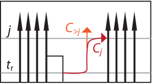
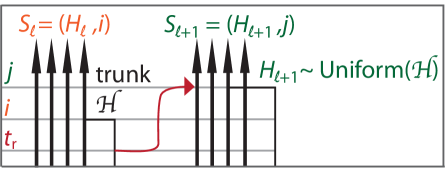
After a sampled lineage recombines at time trsubscript𝑡𝑟t_{r} between loci \ell and +11\ell+1, it will “float” backward in time from the recombination breakpoint until eventually coalescing with a trunk lineage chosen uniformly at random (Figure 1). This implies that ϕ(h,j|h,k)=ϕ(h,j|h′′,k)italic-ϕconditional𝑗superscript𝑘italic-ϕconditional𝑗superscript′′𝑘\phi(h,j|h^{\prime},k)=\phi(h,j|h^{\prime\prime},k) whenever hhsuperscripth^{\prime}\neq h and h′′hsuperscript′′h^{\prime\prime}\neq h, and exploiting this symmetry allows the forward table to be computed in O(nd2L)𝑂𝑛superscript𝑑2𝐿O(nd^{2}L) time. This speed-up was already implemented in the algorithm described in Paul et al. [22].
Refer to caption
Refer to caption
Figure 1: (a). Here, we illustrate a transition from hidden state S=(hn,i)subscript𝑆subscript𝑛𝑖S_{\ell}=(h_{n},i) to hidden state S+1=(hk,j)subscript𝑆1subscript𝑘𝑗S_{\ell+1}=(h_{k},j) that proceeds via recombination at time trsubscript𝑡𝑟t_{r}. The probability of this transition does not depend on the identity of the haplotype hksubscript𝑘h_{k}.(b). As a recombined lineage floats through time interval j𝑗j, it can either coalesce with the trunk (event Cjsubscript𝐶𝑗C_{j}) or keep floating (event C>jsubscript𝐶absent𝑗C_{>j}) and eventually coalesce with the trunk in a more ancient time interval.

Another symmetry of the transition matrix, not exploited previously, can be found by decomposing the transition from locus \ell to locus +11\ell+1 as a sequence of component events. In particular, let Risubscript𝑅𝑖R_{i} be the event that a recombination occurs during time interval i𝑖i, and let R¯¯𝑅\overline{R} be the event that no recombination occurs between \ell and +11\ell+1. Then we have that

ϕ((h,j)(h,k))italic-ϕconditional𝑗superscript𝑘\displaystyle\phi((h,j)\mid(h^{\prime},k)) =1ni=1min(j,k)((Ri,T+1=jT=k)\displaystyle=\frac{1}{n}\sum_{i=1}^{\min(j,k)}\left(\mathbb{P}(R_{i},T_{\ell+1}=j\mid T_{\ell}=k)\right.
+𝟙{(h,j)=(h,k)}(R¯T=k)),\displaystyle+\left.\mathbbm{1}_{\{(h,j)=(h^{\prime},k^{\prime})\}}\mathbb{P}(\overline{R}\mid T_{\ell}=k)\right), (2)

where 𝟙E=1subscript1𝐸1\mathbbm{1}_{E}=1 if the event E𝐸E is true or 00 otherwise. The factor 1/n1𝑛1/n corresponds to the probability that the sampled lineage coalesces with haplotype hh\in\mathcal{H} in the trunk genealogy.

If a recombination occurs in time interval i𝑖i, the sampled lineage will start to “float” freely back in time until it either coalesces in i𝑖i or floats into the next time interval i+1𝑖1i+1 (Figure 1). Specifically, we let C>isubscript𝐶absent𝑖C_{>i} denote the event where the sampled lineage recombines at or before i𝑖i and floats into i+1𝑖1i+1, and Cisubscript𝐶𝑖C_{i} denote the event where the recombined lineage coalesces back in interval i𝑖i. Noting that (Ri,CiT=i)subscript𝑅𝑖conditionalsubscript𝐶𝑖subscript𝑇superscript𝑖\mathbb{P}(R_{i},C_{i}\mid T_{\ell}=i^{\prime}) and (Ri,C>iT=i)subscript𝑅𝑖conditionalsubscript𝐶absent𝑖subscript𝑇superscript𝑖\mathbb{P}(R_{i},C_{>i}\mid T_{\ell}=i^{\prime}) are independent of isuperscript𝑖i^{\prime} whenever i>isuperscript𝑖𝑖i^{\prime}>i, and that coalescence happens as a Markov process backwards in time, we obtain

(Ri,T+1=j\displaystyle\mathbb{P}(R_{i},T_{\ell+1}=j T=k)=𝟙i=j=k(Ri,CiT=i)\displaystyle\mid T_{\ell}=k)=\mathbbm{1}_{i=j=k}\cdot\mathbb{P}(R_{i},C_{i}\mid T_{\ell}=i)
+𝟙i=j<k(Ri,CiT>i)subscript1𝑖𝑗𝑘subscript𝑅𝑖subscript𝐶𝑖ketsubscript𝑇𝑖\displaystyle+\mathbbm{1}_{i=j<k}\cdot\mathbb{P}(R_{i},C_{i}\mid T_{\ell}>i)
+𝟙i=k<j(Ri,C>iT=i)k=ij1(C>k+1C>k)subscript1𝑖𝑘𝑗subscript𝑅𝑖conditionalsubscript𝐶absent𝑖subscript𝑇𝑖superscriptsubscriptproduct𝑘𝑖𝑗1conditionalsubscript𝐶absent𝑘1subscript𝐶absent𝑘\displaystyle+\mathbbm{1}_{i=k<j}\cdot\mathbb{P}(R_{i},C_{>i}\mid T_{\ell}=i)\cdot\prod_{k=i}^{j-1}\mathbb{P}(C_{>k+1}\mid C_{>k})
+𝟙i<min(j,k)(Ri,C>iT>i)k=ij1(C>k+1C>k).subscript1𝑖𝑗𝑘subscript𝑅𝑖subscript𝐶absent𝑖ketsubscript𝑇𝑖superscriptsubscriptproduct𝑘𝑖𝑗1conditionalsubscript𝐶absent𝑘1subscript𝐶absent𝑘\displaystyle+\mathbbm{1}_{i<\min(j,k)}\cdot\mathbb{P}(R_{i},C_{>i}\mid T_{\ell}>i)\cdot\prod_{k=i}^{j-1}\mathbb{P}(C_{>k+1}\mid C_{>k}). (3)

Explicit formulas (specific to the method diCal) for the above terms are provided in the appendix.

By combining (2) with (2.1) and then collecting terms in (1), we can remove the sum over T=ksubscript𝑇𝑘T_{\ell}=k when computing f(x1:+1,S+1)𝑓subscript𝑥:11subscript𝑆1f(x_{1:\ell+1},S_{\ell+1}). In particular, we define additional forward probabilities

f(x1:,T=k)𝑓subscript𝑥:1subscript𝑇𝑘\displaystyle f\left(x_{1:\ell},T_{\ell}=k\right) :=(x1:,T=k)=hf(x1:,S=(h,k)),assignabsentsubscript𝑥:1subscript𝑇𝑘subscriptsuperscript𝑓subscript𝑥:1subscript𝑆superscript𝑘\displaystyle:=\mathbb{P}(x_{1:\ell},T_{\ell}=k)=\sum_{h^{\prime}\in\mathcal{H}}f(x_{1:\ell},S_{\ell}=(h^{\prime},k)), (4)
f(x1:,T>k)𝑓subscript𝑥:1subscript𝑇𝑘\displaystyle f\left(x_{1:\ell},T_{\ell}>k\right) :=(x1:,T>k)=k=k+1dhf(x1:,S=(h,k)),assignabsentsubscript𝑥:1subscript𝑇𝑘superscriptsubscriptsuperscript𝑘𝑘1𝑑subscriptsuperscript𝑓subscript𝑥:1subscript𝑆superscriptsuperscript𝑘\displaystyle:=\mathbb{P}(x_{1:\ell},T_{\ell}>k)=\sum_{k^{\prime}=k+1}^{d}\sum_{h^{\prime}\in\mathcal{H}}f(x_{1:\ell},S_{\ell}=(h^{\prime},k^{\prime})), (5)
f(x1:,Rj,C>j)𝑓subscript𝑥:1subscript𝑅absent𝑗subscript𝐶absent𝑗\displaystyle f\left(x_{1:\ell},R_{\leq j},C_{>j}\right) :=i=1j(x1:,Ri,C>i,,C>j)assignabsentsuperscriptsubscript𝑖1𝑗subscript𝑥:1subscript𝑅𝑖subscript𝐶absent𝑖subscript𝐶absent𝑗\displaystyle:=\sum_{i=1}^{j}\mathbb{P}(x_{1:\ell},R_{i},C_{>i},\ldots,C_{>j}) (6)
=i=1j{[i=i+1j(C>iC>i1)]\displaystyle\phantom{:}=\sum_{i=1}^{j}\Bigg{\{}\bigg{[}\prod_{i^{\prime}=i+1}^{j}\mathbb{P}(C_{>i^{\prime}}\mid C_{>i^{\prime}-1})\bigg{]}
×[f(x1:,T=i)\displaystyle\times\bigg{[}f\left(x_{1:\ell},T_{\ell}=i\right) (Ri,C>iT=i)+f(x1:,T>i)(Ri,C>iT>i)]}.\displaystyle\mathbb{P}(R_{i},C_{>i}\mid T_{\ell}=i)+f\left(x_{1:\ell},T_{\ell}>i\right)\mathbb{P}(R_{i},C_{>i}\mid T_{\ell}>i)\bigg{]}\Bigg{\}}.

Then, (1) can be written as

f(x1:+1,(h,j))𝑓subscript𝑥:11𝑗\displaystyle f(x_{1:\ell+1},(h,j)) =\displaystyle= ξ(x+1h+1,j)[1nf(x1:,Rj1,C>j1)(Cj|C>j1)\displaystyle\xi(x_{\ell+1}\mid h_{\ell+1},j)\cdot\bigg{[}\frac{1}{n}f\left(x_{1:\ell},R_{\leq j-1},C_{>j-1}\right)\mathbb{P}(C_{j}|C_{>j-1}) (7)
+1nf(x1:,T>j)(Rj,CjT>j)1𝑛𝑓subscript𝑥:1subscript𝑇𝑗subscript𝑅𝑗subscript𝐶𝑗ketsubscript𝑇𝑗\displaystyle+\frac{1}{n}f\left(x_{1:\ell},T_{\ell}>j\right)\mathbb{P}(R_{j},C_{j}\mid T_{\ell}>j)
+1nf(x1:,T=j)(Rj,CjT=j)1𝑛𝑓subscript𝑥:1subscript𝑇𝑗subscript𝑅𝑗conditionalsubscript𝐶𝑗subscript𝑇𝑗\displaystyle+\frac{1}{n}f\left(x_{1:\ell},T_{\ell}=j\right)\mathbb{P}(R_{j},C_{j}\mid T_{\ell}=j)
+f(x1:,(h,j))(R¯T=j)].\displaystyle+f(x_{1:\ell},(h,j))\mathbb{P}(\overline{R}\mid T_{\ell}=j)\bigg{]}.

This can be seen by noting that the first three terms in the sum correspond to the terms for i<j𝑖𝑗i<j, i=j<k𝑖𝑗𝑘i=j<k, and i=j=k𝑖𝑗𝑘i=j=k, respectively when putting together (1) and (2). Alternatively, (7) follows from directly considering the probabilistic interpretation of the terms f(x1:,)𝑓subscript𝑥:1f(x_{1:\ell},*) as given by (4), (5), and (6).

The required values of f(x1:,Ri,C>i)𝑓subscript𝑥:1subscript𝑅absent𝑖subscript𝐶absent𝑖f\left(x_{1:\ell},R_{\leq i},C_{>i}\right) and f(x1:,T>i)𝑓subscript𝑥:1subscript𝑇𝑖f\left(x_{1:\ell},T_{\ell}>i\right) can be computed recursively using

f(x1:,T>i)𝑓subscript𝑥:1subscript𝑇𝑖\displaystyle f\left(x_{1:\ell},T_{\ell}>i\right) =\displaystyle= f(x1:,T>i+1)+f(x1:,T=i+1),𝑓subscript𝑥:1subscript𝑇𝑖1𝑓subscript𝑥:1subscript𝑇𝑖1\displaystyle f\left(x_{1:\ell},T_{\ell}>i+1\right)+f\left(x_{1:\ell},T_{\ell}=i+1\right), (8)
f(x1:,Ri,C>i)𝑓subscript𝑥:1subscript𝑅absent𝑖subscript𝐶absent𝑖\displaystyle f\left(x_{1:\ell},R_{\leq i},C_{>i}\right) =\displaystyle= f(x1:,Ri1,C>i1)(C>i|C>i1)𝑓subscript𝑥:1subscript𝑅absent𝑖1subscript𝐶absent𝑖1conditionalsubscript𝐶absent𝑖subscript𝐶absent𝑖1\displaystyle f\left(x_{1:\ell},R_{\leq i-1},C_{>i-1}\right)\mathbb{P}(C_{>i}|C_{>i-1}) (9)
+f(x1:,T=i)(Ri,C>iT=i)𝑓subscript𝑥:1subscript𝑇𝑖subscript𝑅𝑖conditionalsubscript𝐶absent𝑖subscript𝑇𝑖\displaystyle+f\left(x_{1:\ell},T_{\ell}=i\right)\mathbb{P}(R_{i},C_{>i}\mid T_{\ell}=i)
+f(x1:,T>i)(Ri,C>iT>i),𝑓subscript𝑥:1subscript𝑇𝑖subscript𝑅𝑖subscript𝐶absent𝑖ketsubscript𝑇𝑖\displaystyle+f\left(x_{1:\ell},T_{\ell}>i\right)\mathbb{P}(R_{i},C_{>i}\mid T_{\ell}>i),

with the base cases

f(x1:,T>d)𝑓subscript𝑥:1subscript𝑇𝑑\displaystyle f\left(x_{1:\ell},T_{\ell}>d\right) =\displaystyle= 0,0\displaystyle 0,
f(x1:,R1,C>1)𝑓subscript𝑥:1subscript𝑅absent1subscript𝐶absent1\displaystyle f\left(x_{1:\ell},R_{\leq 1},C_{>1}\right) =\displaystyle= f(x1:,T>1)(R1,C>1T>1)𝑓subscript𝑥:1subscript𝑇1subscript𝑅1subscript𝐶absent1ketsubscript𝑇1\displaystyle f\left(x_{1:\ell},T_{\ell}>1\right)\mathbb{P}(R_{1},C_{>1}\mid T_{\ell}>1)
+f(x1:,T=1)(R1,C>1T=1).𝑓subscript𝑥:1subscript𝑇1subscript𝑅1conditionalsubscript𝐶absent1subscript𝑇1\displaystyle+f\left(x_{1:\ell},T_{\ell}=1\right)\mathbb{P}(R_{1},C_{>1}\mid T_{\ell}=1).

Hence, using the recursions (7),  (8), and (9), it is possible to compute the entire forward DP table {f(x1:,S)}=1Lsuperscriptsubscript𝑓subscript𝑥:1subscript𝑆1𝐿\{f(x_{1:\ell},S_{\ell})\}_{\ell=1}^{L} exactly in O(ndL)𝑂𝑛𝑑𝐿O(ndL) time.

2.2 A linear-time backward algorithm

The backward DP table {b(x+1:LS)}𝑏conditionalsubscript𝑥:1𝐿subscript𝑆\{b(x_{\ell+1:L}\mid S_{\ell})\} can be also computed in O(ndL)𝑂𝑛𝑑𝐿O(ndL) time. Given the linear-time forward algorithm discussed in the previous section, the easiest way to compute the backward DP table is as follows: Let x(r)=x1(r),x2(r),,xL(r)=xL,xL1,,x1formulae-sequencesuperscript𝑥𝑟subscriptsuperscript𝑥𝑟1subscriptsuperscript𝑥𝑟2subscriptsuperscript𝑥𝑟𝐿subscript𝑥𝐿subscript𝑥𝐿1subscript𝑥1x^{(r)}=x^{(r)}_{1},x^{(r)}_{2},\ldots,x^{(r)}_{L}=x_{L},x_{L-1},\ldots,x_{1} denote the reversed x𝑥x and let S(r)subscriptsuperscript𝑆𝑟S^{(r)}_{\ell} denote the hidden states for the HMM generating x(r)superscript𝑥𝑟x^{(r)}. Then, since the coalescent is reversible along the sequence,

b(x+1:L(r)s)=(x+1:L(r),S=s)ζ(s)=(x:L(r),S=s)ξ(x(r)s)ζ(s)=f(x1:L+1(r),SL+1(r)=s)ξ(x(r)s)ζ(s).𝑏conditionalsubscriptsuperscript𝑥𝑟:1𝐿𝑠subscriptsuperscript𝑥𝑟:1𝐿subscript𝑆𝑠𝜁𝑠subscriptsuperscript𝑥𝑟:𝐿subscript𝑆𝑠𝜉conditionalsubscriptsuperscript𝑥𝑟𝑠𝜁𝑠𝑓subscriptsuperscript𝑥𝑟:1𝐿1subscriptsuperscript𝑆𝑟𝐿1𝑠𝜉conditionalsubscriptsuperscript𝑥𝑟𝑠𝜁𝑠\displaystyle b(x^{(r)}_{\ell+1:L}\mid s)=\frac{\mathbb{P}(x^{(r)}_{\ell+1:L},S_{\ell}=s)}{\zeta(s)}=\frac{\mathbb{P}(x^{(r)}_{\ell:L},S_{\ell}=s)}{\xi(x^{(r)}_{\ell}\mid s)\zeta(s)}=\frac{f(x^{(r)}_{1:L-\ell+1},S^{(r)}_{L-\ell+1}=s)}{\xi(x^{(r)}_{\ell}\mid s)\zeta(s)}.

3 Linear-Time EM via an Augmented HMM

The primary application of PSMC and diCal is parameter estimation, specifically the estimation of demographic parameters such as changing population sizes. This is done through a maximum likelihood framework with the expectation maximization (EM) algorithm. In this section, we describe how to speed up the EM algorithm to work in linear time.

3.1 The standard EM algorithm with O(d2)𝑂superscript𝑑2O(d^{2}) time complexity

Let ΘΘ\Theta denote the parameters we wish to estimate, and Θ^^Θ\hat{\Theta} denote the maximum likelihood estimate:

Θ^=argmaxΘ(Θ)=argmaxΘΘ(x1:L).^ΘsubscriptsuperscriptΘsuperscriptΘsubscriptsuperscriptΘsubscriptsuperscriptΘsubscript𝑥:1𝐿\displaystyle\hat{\Theta}=\arg\max_{\Theta^{\prime}}\mathcal{L}(\Theta^{\prime})=\arg\max_{\Theta^{\prime}}\mathbb{P}_{\Theta^{\prime}}(x_{1:L}).

To find Θ^^Θ\hat{\Theta}, we pick some initial value Θ(0)superscriptΘ0\Theta^{(0)}, and then iteratively solve for Θ(t)superscriptΘ𝑡\Theta^{(t)} according to

Θ(t)=argmaxΘ𝔼S1:L;Θ(t1)[logΘ(x1:L,S1:L)x1:L],superscriptΘ𝑡subscriptsuperscriptΘsubscript𝔼subscript𝑆:1𝐿superscriptΘ𝑡1delimited-[]conditionalsubscriptsuperscriptΘsubscript𝑥:1𝐿subscript𝑆:1𝐿subscript𝑥:1𝐿\displaystyle\Theta^{(t)}=\arg\max_{\Theta^{\prime}}\mathbb{E}_{S_{1:L};\Theta^{(t-1)}}[\log\mathbb{P}_{\Theta^{\prime}}(x_{1:L},S_{1:L})\mid x_{1:L}],

where S1:L:=S1,,SLassignsubscript𝑆:1𝐿subscript𝑆1subscript𝑆𝐿S_{1:L}:=S_{1},\ldots,S_{L}. The sequence Θ(0),Θ(1),superscriptΘ0superscriptΘ1\Theta^{(0)},\Theta^{(1)},\ldots is then guaranteed to converge to a local maximum of the surface (Θ)Θ\mathcal{L}(\Theta).

Since (x1:L,S1:L)subscript𝑥:1𝐿subscript𝑆:1𝐿(x_{1:L},S_{1:L}) forms an HMM, the joint likelihood (x1:L,S1:L)subscript𝑥:1𝐿subscript𝑆:1𝐿\mathbb{P}(x_{1:L},S_{1:L}) can be written as

Θ(x1:L,S1:L)subscriptsuperscriptΘsubscript𝑥:1𝐿subscript𝑆:1𝐿\displaystyle\mathbb{P}_{\Theta^{\prime}}(x_{1:L},S_{1:L}) =ζΘ(S1)[=1LξΘ(xS)][=2LϕΘ(SS1)].absentsubscript𝜁superscriptΘsubscript𝑆1delimited-[]superscriptsubscriptproduct1𝐿subscript𝜉superscriptΘconditionalsubscript𝑥subscript𝑆delimited-[]superscriptsubscriptproduct2𝐿subscriptitalic-ϕsuperscriptΘconditionalsubscript𝑆subscript𝑆1\displaystyle=\zeta_{\Theta^{\prime}}(S_{1})\left[\prod_{\ell=1}^{L}\xi_{\Theta^{\prime}}(x_{\ell}\mid S_{\ell})\right]\left[\prod_{\ell=2}^{L}\phi_{\Theta^{\prime}}(S_{\ell}\mid S_{\ell-1})\right].

Letting 𝔼[#:Ex1:L]\mathbb{E}[\#\ell:E\mid x_{1:L}] denote the posterior expected number of loci where event E𝐸E occurs, and π(x):=(x)=sf(x1:L,s)assign𝜋𝑥𝑥subscript𝑠𝑓subscript𝑥:1𝐿𝑠\pi(x):=\mathbb{P}(x)=\sum_{s}f(x_{1:L},s) denote the total probability of observing x𝑥x, we then have

𝔼S1:L;Θ[logΘ(x1:L,S1:L)|x1:L]subscript𝔼subscript𝑆:1𝐿Θdelimited-[]conditionalsubscriptsuperscriptΘsubscript𝑥:1𝐿subscript𝑆:1𝐿subscript𝑥:1𝐿\displaystyle\mathbb{E}_{S_{1:L};\Theta}\big{[}\log\mathbb{P}_{\Theta^{\prime}}(x_{1:L},S_{1:L})\big{|}x_{1:L}\big{]}
=\displaystyle= s(logζΘ(s))Θ(S1=s|x1:L)subscript𝑠subscript𝜁superscriptΘ𝑠subscriptΘsubscript𝑆1conditional𝑠subscript𝑥:1𝐿\displaystyle\sum_{s}\left(\log\zeta_{\Theta^{\prime}}(s)\right)\mathbb{P}_{\Theta}(S_{1}=s|x_{1:L})
+(h,i)a,b𝒜(logξΘ(a|b,i))𝔼Θ[#:{S=(h,i),h=b,x=a}|x1:L]\displaystyle\qquad+\sum_{(h,i)}\sum_{a,b\in\mathcal{A}}\left(\log\xi_{\Theta^{\prime}}(a|b,i)\right)\mathbb{E}_{\Theta}\big{[}\#\ell:\{S_{\ell}=(h,i),h_{\ell}=b,x_{\ell}=a\}\big{|}x_{1:L}\big{]}
+s,s(logϕΘ(ss))𝔼Θ[#:{S1=s,S=s}|x1:L]\displaystyle\qquad+\sum_{s,s^{\prime}}\left(\log\phi_{\Theta^{\prime}}(s^{\prime}\mid s)\right)\mathbb{E}_{\Theta}\big{[}\#\ell:\{S_{\ell-1}=s,S_{\ell}=s^{\prime}\}\big{|}x_{1:L}\big{]}
=\displaystyle= 1πΘ(x)[s(logζΘ(s))fΘ(x1,s)bΘ(x2:L|s)\displaystyle\frac{1}{\pi_{\Theta}(x)}\Bigg{[}\sum_{s}\left(\log\zeta_{\Theta^{\prime}}(s)\right)f_{\Theta}(x_{1},s)b_{\Theta}(x_{2:L}|s)
+(h,i)a,b𝒜(logξΘ(a|b,i)):x=ah=bfΘ(x1:,(h,i))bΘ(x+1:L|h,i)subscript𝑖subscript𝑎𝑏𝒜subscript𝜉superscriptΘconditional𝑎𝑏𝑖subscript:subscript𝑥𝑎subscript𝑏subscript𝑓Θsubscript𝑥:1𝑖subscript𝑏Θconditionalsubscript𝑥:1𝐿𝑖\displaystyle\qquad+\sum_{(h,i)}\sum_{a,b\in\mathcal{A}}\left(\log\xi_{\Theta^{\prime}}(a|b,i)\right)\!\!\sum_{\begin{subarray}{c}\ell:x_{\ell}=a\\ h_{\ell}=b\end{subarray}}\!\!f_{\Theta}(x_{1:\ell},(h,i))b_{\Theta}(x_{\ell+1:L}|h,i)
+s,s(logϕΘ(ss))(=1L1fΘ(x1:,s)ϕΘ(ss)ξΘ(x+1s)bΘ(x+2:Ls))].\displaystyle+\sum_{s,s^{\prime}}\left(\log\phi_{\Theta^{\prime}}(s^{\prime}\mid s)\right)\left(\sum_{\ell=1}^{L-1}f_{\Theta}(x_{1:\ell},s)\phi_{\Theta}(s^{\prime}\mid s)\xi_{\Theta}(x_{\ell+1}\mid s^{\prime})b_{\Theta}(x_{\ell+2:L}\mid s^{\prime})\right)\Bigg{]}. (10)

Note that we have to compute the term fΘ(x1:,s)ϕΘ(ss)ξΘ(x+1s)subscriptsubscript𝑓Θsubscript𝑥:1𝑠subscriptitalic-ϕΘconditionalsuperscript𝑠𝑠subscript𝜉Θconditionalsubscript𝑥1superscript𝑠\sum_{\ell}f_{\Theta}(x_{1:\ell},s)\phi_{\Theta}(s^{\prime}\mid s)\xi_{\Theta}(x_{\ell+1}\mid s^{\prime}) bΘ(x+2:Ls)subscript𝑏Θconditionalsubscript𝑥:2𝐿superscript𝑠b_{\Theta}(x_{\ell+2:L}\mid s^{\prime}) for every pair of states s,s𝑠superscript𝑠s,s^{\prime}, which makes computing the EM objective function quadratic in the number d𝑑d of discretization time intervals, despite the fact that we computed the forward and backward tables in linear time.

3.2 A linear-time EM algorithm

By augmenting our HMM to condition on whether recombination occurred between loci \ell and +11\ell+1, the EM algorithm can be sped up to be linear in d𝑑d. We now describe this augmented HMM. Let \mathcal{M} denote our original HMM, with states S1:Lsubscript𝑆:1𝐿S_{1:L} and observations x1:Lsubscript𝑥:1𝐿x_{1:L}. Between loci \ell and +11\ell+1, define

l,l+1={R¯,if no recombination,Ri,if recombination occurred at time i.subscript𝑙𝑙1cases¯𝑅if no recombination,subscript𝑅𝑖if recombination occurred at time 𝑖\mathcal{R}_{l,l+1}=\begin{cases}\overline{R},&\text{if no recombination,}\\ R_{i},&\text{if recombination occurred at time }i.\end{cases}

Now let S1=S1subscriptsuperscript𝑆1subscript𝑆1S^{*}_{1}=S_{1}, and S=(1,,S)subscriptsuperscript𝑆subscript1subscript𝑆S^{*}_{\ell}=(\mathcal{R}_{\ell-1,\ell},S_{\ell}) for >11\ell>1. We let superscript\mathcal{M}^{*} be the HMM with hidden variables S1:L=S1,,SLsubscriptsuperscript𝑆:1𝐿subscriptsuperscript𝑆1subscriptsuperscript𝑆𝐿S^{*}_{1:L}=S^{*}_{1},\ldots,S^{*}_{L}, observations x1:Lsubscript𝑥:1𝐿x_{1:L}, transition probabilities (SS1)=(SS1)conditionalsubscriptsuperscript𝑆subscriptsuperscript𝑆1conditionalsubscriptsuperscript𝑆subscript𝑆1\mathbb{P}(S^{*}_{\ell}\mid S^{*}_{\ell-1})=\mathbb{P}(S^{*}_{\ell}\mid S_{\ell-1}), and emission probabilities (xS)=(xS)conditionalsubscript𝑥subscriptsuperscript𝑆conditionalsubscript𝑥subscript𝑆\mathbb{P}(x_{\ell}\mid S^{*}_{\ell})=\mathbb{P}(x_{\ell}\mid S_{\ell}). Note that the probability of observing the data is the same under \mathcal{M} and superscript\mathcal{M}^{*}, i.e.,

(Θ)Θ\displaystyle\mathcal{L}(\Theta) =Θ(x1:L)=Θ(x1:L),absentsubscriptΘconditionalsubscript𝑥:1𝐿subscriptΘconditionalsubscript𝑥:1𝐿superscript\displaystyle=\mathbb{P}_{\Theta}(x_{1:L}\mid\mathcal{M})=\mathbb{P}_{\Theta}(x_{1:L}\mid\mathcal{M}^{*}),

and so we may find a local maximum of (Θ)Θ\mathcal{L}(\Theta) by applying the EM algorithm to the augmented HMM superscript\mathcal{M}^{*}, instead of to the original HMM \mathcal{M}.

To compute the EM objective function for superscript\mathcal{M}^{*}, we start by noting that the joint likelihood is

(x1:L,S1:L)subscript𝑥:1𝐿subscriptsuperscript𝑆:1𝐿\displaystyle\mathbb{P}(x_{1:L},S^{*}_{1:L}) =ζ(S1)[=1Lξ(xS)][:,+1=R¯(R¯T)]absent𝜁subscript𝑆1delimited-[]superscriptsubscriptproduct1𝐿𝜉conditionalsubscript𝑥subscript𝑆delimited-[]subscriptproduct:subscript1¯𝑅conditional¯𝑅subscript𝑇\displaystyle=\zeta(S_{1})\bigg{[}\prod_{\ell=1}^{L}\xi(x_{\ell}\mid S_{\ell})\bigg{]}\bigg{[}\prod_{\begin{subarray}{c}\ell:\mathcal{R}_{\ell,\ell+1}=\overline{R}\end{subarray}}\mathbb{P}(\overline{R}\mid T_{\ell})\bigg{]} (11)
×[i=1d:,+1=Ri(Ri,T+1T)](1n)#:,+1R¯,absentdelimited-[]superscriptsubscriptproduct𝑖1𝑑subscriptproduct:subscript1subscript𝑅𝑖subscript𝑅𝑖conditionalsubscript𝑇1subscript𝑇superscript1𝑛:#subscript1¯𝑅\displaystyle\qquad\qquad\times\bigg{[}\prod_{i=1}^{d}\prod_{\begin{subarray}{c}\ell:\mathcal{R}_{\ell,\ell+1}=R_{i}\end{subarray}}\mathbb{P}(R_{i},T_{\ell+1}\mid T_{\ell})\bigg{]}\left(\frac{1}{n}\right)^{\#\ell:\mathcal{R}_{\ell,\ell+1}\neq\overline{R}},

where we decomposed the joint likelihood into the initial probability, the emission probabilities, the transitions without recombination, and the transitions with recombination. We note that the initial probability can be decomposed as

ζ(S1=(h,j))𝜁subscript𝑆1𝑗\displaystyle\zeta(S_{1}=(h,j)) =1n[i=1j1(C>iC>i1)](CjC>j1),absent1𝑛delimited-[]superscriptsubscriptproduct𝑖1𝑗1conditionalsubscript𝐶absent𝑖subscript𝐶absent𝑖1conditionalsubscript𝐶𝑗subscript𝐶absent𝑗1\displaystyle=\frac{1}{n}\Bigg{[}\prod_{i=1}^{j-1}\mathbb{P}(C_{>i}\mid C_{>i-1})\Bigg{]}\mathbb{P}(C_{j}\mid C_{>j-1}), (12)

and from (2.1), we decompose the product of transition recombination probabilities as

i=1d:,+1=Ri(Ri,T+1T)superscriptsubscriptproduct𝑖1𝑑subscriptproduct:subscript1subscript𝑅𝑖subscript𝑅𝑖conditionalsubscript𝑇1subscript𝑇\displaystyle\prod_{i=1}^{d}\prod_{\begin{subarray}{c}\ell:\mathcal{R}_{\ell,\ell+1}=R_{i}\end{subarray}}\mathbb{P}(R_{i},T_{\ell+1}\mid T_{\ell}) =i=1d{[:,+1=RiT=T+1=i(Ri,CiT=i)]\displaystyle=\prod_{i=1}^{d}\Bigg{\{}\bigg{[}\prod_{\begin{subarray}{c}\ell:\mathcal{R}_{\ell,\ell+1}=R_{i}\\ T_{\ell}=T_{\ell+1}=i\end{subarray}}\mathbb{P}(R_{i},C_{i}\mid T_{\ell}=i)\bigg{]}
×[:,+1=RiT>T+1=i(Ri,CiT>i)][:,+1=RiT+1>T=i(Ri,C>iT=i)]absentdelimited-[]subscriptproduct:subscript1subscript𝑅𝑖subscript𝑇subscript𝑇1𝑖subscript𝑅𝑖subscript𝐶𝑖ketsubscript𝑇𝑖delimited-[]subscriptproduct:subscript1subscript𝑅𝑖subscript𝑇1subscript𝑇𝑖subscript𝑅𝑖conditionalsubscript𝐶absent𝑖subscript𝑇𝑖\displaystyle\qquad\times\bigg{[}\prod_{\begin{subarray}{c}\ell:\mathcal{R}_{\ell,\ell+1}=R_{i}\\ T_{\ell}>T_{\ell+1}=i\end{subarray}}\mathbb{P}(R_{i},C_{i}\mid T_{\ell}>i)\bigg{]}\bigg{[}\prod_{\begin{subarray}{c}\ell:\mathcal{R}_{\ell,\ell+1}=R_{i}\\ T_{\ell+1}>T_{\ell}=i\end{subarray}}\mathbb{P}(R_{i},C_{>i}\mid T_{\ell}=i)\bigg{]}
×[:,+1=RiT,T+1>i(Ri,C>iT>i)][:T+1>i,+1R<i(C>iC>i1)]absentdelimited-[]subscriptproduct:subscript1subscript𝑅𝑖subscript𝑇subscript𝑇1𝑖subscript𝑅𝑖subscript𝐶absent𝑖ketsubscript𝑇𝑖delimited-[]subscriptproduct:subscript𝑇1𝑖subscript1subscript𝑅absent𝑖conditionalsubscript𝐶absent𝑖subscript𝐶absent𝑖1\displaystyle\qquad\times\bigg{[}\prod_{\begin{subarray}{c}\ell:\mathcal{R}_{\ell,\ell+1}=R_{i}\\ T_{\ell},T_{\ell+1}>i\end{subarray}}\mathbb{P}(R_{i},C_{>i}\mid T_{\ell}>i)\bigg{]}\bigg{[}\prod_{\begin{subarray}{c}\ell:T_{\ell+1}>i\\ \mathcal{R}_{\ell,\ell+1}\in R_{<i}\end{subarray}}\mathbb{P}(C_{>i}\mid C_{>i-1})\bigg{]}
×[:T+1=i,+1R<i(CiC>i1)]},\displaystyle\qquad\times\bigg{[}\prod_{\begin{subarray}{c}\ell:T_{\ell+1}=i\\ \mathcal{R}_{\ell,\ell+1}\in R_{<i}\end{subarray}}\mathbb{P}(C_{i}\mid C_{>i-1})\bigg{]}\Bigg{\}}, (13)

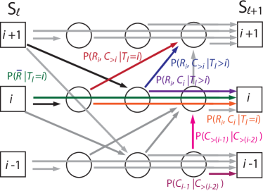
where R<i:=j<iRjassignsubscript𝑅absent𝑖subscript𝑗𝑖subscript𝑅𝑗R_{<i}:=\cup_{j<i}R_{j}. Figure 2 shows a graphical representation for the transitions of superscript\mathcal{M}^{*}.

Refer to caption
Figure 2: This diagram illustrates the flow of transition probabilities through the augmented HMM. Lineages may transition between different coalescence times at loci \ell and +11\ell+1 by recombining and passing through the floating states represented by circles. Each interval contains three distinct floating states to capture the the dependence of recombination and coalescence probabilities on whether any of these events occur during the same time interval.

By plugging (12) and (13) into (11), then taking the posterior expected logarithm of (11), we obtain the EM objective function for superscript\mathcal{M}^{*}:

𝔼S1:L;Θ[logΘ(x1:L,S1:L)x1:L]subscript𝔼subscriptsuperscript𝑆:1𝐿Θdelimited-[]conditionalsubscriptsuperscriptΘsubscript𝑥:1𝐿subscriptsuperscript𝑆:1𝐿subscript𝑥:1𝐿\displaystyle\mathbb{E}_{S^{*}_{1:L};\Theta}\Big{[}\log\mathbb{P}_{\Theta^{\prime}}(x_{1:L},S^{*}_{1:L})\mid x_{1:L}\Big{]} =Llogn+i=1dqi(Θ,Θ),absent𝐿𝑛superscriptsubscript𝑖1𝑑subscript𝑞𝑖ΘsuperscriptΘ\displaystyle=-L\log n+\sum_{i=1}^{d}q_{i}(\Theta,\Theta^{\prime}), (14)

where

qisubscript𝑞𝑖\displaystyle q_{i} (Θ,Θ):=a,b𝒜[logξΘ(ab,i)πΘ(x):x=ah:h=bfΘ(x1:,(h,i))bΘ(x+1:L(h,i))]assignΘsuperscriptΘsubscript𝑎𝑏𝒜delimited-[]subscript𝜉superscriptΘconditional𝑎𝑏𝑖subscript𝜋Θ𝑥subscript:subscript𝑥𝑎subscript:subscript𝑏subscript𝑓Θsubscript𝑥:1𝑖subscript𝑏Θconditionalsubscript𝑥:1𝐿𝑖\displaystyle(\Theta,\Theta^{\prime}):=\sum_{a,b\in\mathcal{A}}\Bigg{[}\frac{\log\xi_{\Theta^{\prime}}(a\mid b,i)}{\pi_{\Theta}(x)}\sum_{\begin{subarray}{c}\ell:x_{\ell}=a\end{subarray}}\sum_{h:h_{\ell}=b}f_{\Theta}(x_{1:\ell},(h,i))b_{\Theta}(x_{\ell+1:L}\mid(h,i))\Bigg{]}
+(logΘ(R¯T=i)+logn)𝔼Θ[#:{,+1=R¯,T=i}x1:L]\displaystyle+\left(\log\mathbb{P}_{\Theta^{\prime}}(\overline{R}\mid T=i)+\log n\right)\mathbb{E}_{\Theta}\Big{[}\#\ell:\{\mathcal{R}_{\ell,\ell+1}=\overline{R},T_{\ell}=i\}\mid x_{1:L}\Big{]}
+(logΘ(Ri,CiT=i))𝔼Θ[#:{,+1=Ri,T=T+1=i}x1:L]\displaystyle+\left(\log\mathbb{P}_{\Theta^{\prime}}(R_{i},C_{i}\mid T=i)\right)\mathbb{E}_{\Theta}\Big{[}\#\ell:\{\mathcal{R}_{\ell,\ell+1}=R_{i},T_{\ell}=T_{\ell+1}=i\}\mid x_{1:L}\Big{]}
+(logΘ(Ri,CiT>i))𝔼Θ[#:{,+1=Ri,T>T+1=i}x1:L]\displaystyle+\left(\log\mathbb{P}_{\Theta^{\prime}}(R_{i},C_{i}\mid T>i)\right)\mathbb{E}_{\Theta}\Big{[}\#\ell:\{\mathcal{R}_{\ell,\ell+1}=R_{i},T_{\ell}>T_{\ell+1}=i\}\mid x_{1:L}\Big{]}
+(logΘ(Ri,C>iT=i))𝔼Θ[#:{,+1=Ri,T+1>T=i}x1:L]\displaystyle+\left(\log\mathbb{P}_{\Theta^{\prime}}(R_{i},C_{>i}\mid T=i)\right)\mathbb{E}_{\Theta}\Big{[}\#\ell:\{\mathcal{R}_{\ell,\ell+1}=R_{i},T_{\ell+1}>T_{\ell}=i\}\mid x_{1:L}\Big{]}
+(logΘ(Ri,C>iT>i))𝔼Θ[#:{,+1=Ri,T>i,T+1>i}x1:L]\displaystyle+\left(\log\mathbb{P}_{\Theta^{\prime}}(R_{i},C_{>i}\mid T>i)\right)\mathbb{E}_{\Theta}\Big{[}\#\ell:\{\mathcal{R}_{\ell,\ell+1}=R_{i},T_{\ell}>i,T_{\ell+1}>i\}\mid x_{1:L}\Big{]}
+(logΘ(C>iC>i1))𝔼Θ[#:{,+1R<i,T+1>i}x1:L]\displaystyle+\left(\log\mathbb{P}_{\Theta^{\prime}}(C_{>i}\mid C_{>i-1})\right)\mathbb{E}_{\Theta}\Big{[}\#\ell:\{\mathcal{R}_{\ell,\ell+1}\in R_{<i},T_{\ell+1}>i\}\mid x_{1:L}\Big{]}
+(logΘ(CiC>i1))𝔼Θ[#:{,+1R<i,T+1=i}x1:L]\displaystyle+\left(\log\mathbb{P}_{\Theta^{\prime}}(C_{i}\mid C_{>i-1})\right)\mathbb{E}_{\Theta}\Big{[}\#\ell:\{\mathcal{R}_{\ell,\ell+1}\in R_{<i},T_{\ell+1}=i\}\mid x_{1:L}\Big{]}
+Θ(T1>ix1:L)+Θ(T1=ix1:L).subscriptΘsubscript𝑇1conditional𝑖subscript𝑥:1𝐿subscriptΘsubscript𝑇1conditional𝑖subscript𝑥:1𝐿\displaystyle+\mathbb{P}_{\Theta}(T_{1}>i\mid x_{1:L})+\mathbb{P}_{\Theta}(T_{1}=i\mid x_{1:L}). (15)

The computation time for each of the posterior expectations 𝔼Θ[#:x1:L]\mathbb{E}_{\Theta}[\#\ell:*\mid x_{1:L}] and Θ(T1x1:L)subscriptΘconditionalsubscript𝑇1subscript𝑥:1𝐿\mathbb{P}_{\Theta}(T_{1}\mid x_{1:L}) does not depend on d𝑑d; full expressions are listed in the appendix. Hence, the number of operations needed to evaluate (14) is linear in d𝑑d.

We note another attractive property of (14). By decomposing the EM objective function into a sum of terms qi(Θ,Θ)subscript𝑞𝑖ΘsuperscriptΘq_{i}(\Theta,\Theta^{\prime}), we obtain a natural strategy for searching through the parameter space. In particular, one can attempt to find the argmaxΘsubscriptsuperscriptΘ\arg\max_{\Theta^{\prime}} of (14) by optimizing the qi(Θ,Θ)subscript𝑞𝑖ΘsuperscriptΘq_{i}(\Theta,\Theta^{\prime}) one at a time in i𝑖i. In fact, for the problem of estimating changing population sizes, qi(Θ,Θ)subscript𝑞𝑖ΘsuperscriptΘq_{i}(\Theta,\Theta^{\prime}) depends on ΘsuperscriptΘ\Theta^{\prime} almost entirely through a single parameter (the population size λisuperscriptsubscript𝜆𝑖\lambda_{i}^{\prime} in interval i𝑖i), and we pursue a strategy of iteratively solving for λisuperscriptsubscript𝜆𝑖\lambda_{i}^{\prime} while holding the other coordinates of ΘsuperscriptΘ\Theta^{\prime} fixed, thus reducing a multivariate optimization problem into a sequence of univariate optimization problems.

Although both the linear and quadratic EM procedures are guaranteed to converge to local maxima of (Θ)Θ\mathcal{L}(\Theta), they may have different rates of convergence, and may converge to different local maxima. The search paths of the two EM algorithms may differ for two reasons: first, the intermediate objective functions (10) and (14) are not equal, and secondly, as discussed above, we use different search strategies to find the optima of (10) and (14). We have no proven guarantee that either search should perform better than the other, but our observations indicate that the linear-time EM algorithm typically converges to a value of ΘΘ\Theta with a equal or higher value of (Θ)Θ\mathcal{L}(\Theta) than the quadratic-time algorithm, in a fraction of the time (see Figure 5 for an example).

4 Results

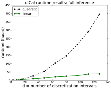
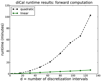
To confirm the decrease in runtime, we ran the linear-time diCal method on simulated data with L=2𝐿2L=2 Mb of loci and 222 haplotypes (in which case diCal is equivalent to PSMC), using d=2,4,8,16,32,48,64,80,96,112,128𝑑248163248648096112128d=2,4,8,16,32,48,64,80,96,112,128 discretization intervals. To simulate the data, we used ms [14] with a population-scaled recombination rate ρ=0.0005𝜌0.0005\rho=0.0005 to generate an ARG, and then added mutations using a population-scaled mutation rate of θ=0.0029𝜃0.0029\theta=0.0029 and a finite-sites mutation matrix described in Sheehan et al. [24]. Figure 3 shows the time required to compute the table of forward probabilities. We also measured the time required for one EM iteration and then extrapolated to 20 iterations to approximate the time required to estimate an effective population size history (Figure 3). In both figures, the linear runtime of our new algorithm is apparent and significantly improves our ability to increase the number of discretization intervals.

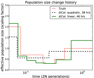
To assess the gain in accuracy of population size estimates that is afforded by more discretization intervals, we ran both the linear- and quadratic-time methods on simulated data with 101010 haplotypes and L=2𝐿2L=2 Mb. The conditional sampling distribution was used in a leave-one-out composite likelihood approach [24] in this experiment. To run each method for roughly the same amount of time (40absent40\approx 40 hours), we used d=9𝑑9d=9 for the quadratic method and d=21𝑑21d=21 for the linear method. For both methods, we ran the EM for 20 iterations and inferred d/3𝑑3d/3 size change parameters. As measured by the PSMC error function, which integrates the absolute value of the difference between the true size function and the estimated size function [15], larger values of d𝑑d permit the inference of more accurate histories.
Refer to caption
Refer to caption
Figure 3: Runtime results on simulated data with L=2𝐿2L=2 Mb and 222 haplotypes, for varying number d𝑑d of discretization intervals. 3 Runtime results (in minutes) for the forward computation. 3 Runtime results (in hours) for the entire EM inference algorithm (20 iterations) extrapolated from the time for one iteration.
Refer to caption
Refer to caption
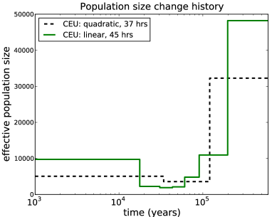
Figure 4: Effective population size change history results. The speedup from the linear method allows us to use a finer discretization (d=21𝑑21d=21) than the quadratic method (d=9𝑑9d=9) for about the same amount of runtime. 4 Results on simulated data with L=2𝐿2L=2~{}Mb and 101010 haplotypes. Using the quadratic method with d=9𝑑9d=9, the error was 0.148. Using the linear method with d=21𝑑21d=21, the error dropped to 0.079. 4 Results on 101010 European haplotypes over a 222 Mb region of chromosome 1. The out-of-Africa bottleneck is very apparent with d=21𝑑21d=21, but is not as well characterized for d=9𝑑9d=9.

We also ran our method on 101010 CEU haplotypes (Utah residents of European descent) sequenced during Phase I of the the 1000 Genomes Project [26] (Figure 4). We can see that for the quadratic method with d=9𝑑9d=9, we are unable to fully characterize the out-of-Africa bottleneck. In the same amount of computational time, we can run the linear method with d=21𝑑21d=21 and easily capture this feature. The disagreement in the ancient past between the two methods is most likely due to diCal’s lack of power in the ancient past when there are not many coalescence events. Using a leave-one-out approach with 101010 haplotypes, the coalescence events in the ancient past tend to be few and unevenly spaced, resulting in a less confident inference.
Refer to caption
Refer to caption
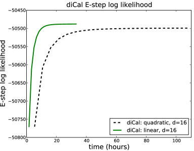
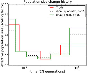
Figure 5: Results on simulated data, using the same discretization for the linear and quadratic methods. Each method was run for 20 iterations. 5 The log likelihood of the EM algorithm, plotted against time, for both the linear and quadratic methods. 5 Population size change history results for the linear and quadratic methods, run with the same discretization using d=16𝑑16d=16 and estimating 666 parameters.

The runtime of the full EM algorithm depends on the convergence of the M-step, which can be variable. Occasionally we observed convergence issues for the quadratic method, which requires a multivariate optimization routine. For the linear method, we used the univariate Brent optimization routine from Apache Math Commons (http://commons.apache.org/proper/commons-math/), which converges quickly and to a large extent avoids local maxima.

To examine the convergence of the two EM algorithms, we ran the linear and quadratic methods on the simulated data with 101010 haplotypes and the same number of intervals d=16𝑑16d=16. We examine the likelihoods in Figure 5. The linear method reaches parameter estimates of higher likelihood, although it is unclear whether the two methods have found different local maxima, or whether the quadratic method is approaching the same maximum more slowly. Figure 5 shows the inferred population sizes for each method, which although similar, are not identical.

We have also looked at the amount of memory required for each method, and although the difference is small, the linear method does require more memory to store the augmented forward and backward tables. A more thorough investigation of memory requirements will be important as the size of the data continues to increase.

5 Discussion

The improvement to diCal described in this paper will enable users to analyze larger datasets and infer more detailed demographic histories. This is especially important given that large datasets are needed to distinguish between histories with subtle or recent differences. By using samples of 10 haplotypes rather than 2, diCal v1.0 [24] was able to distinguish between histories that diverged from each other less than 0.10.10.1 coalescent time units ago, in which period PSMC tends to exhibit runaway behavior and hence cannot produce reliable population size estimates. The faster algorithm described here can handle samples of 30 haplotypes with equivalent computing resources. Our results indicate that this improves the method’s ability to resolve rapid, recent demographic shifts.

In organisms where multiple sequenced genomes are not available, the resources freed up by O(d)𝑂𝑑O(d) HMM decoding could be used to avoid grouping sites into 100-locus bins. This binning technique is commonly used to improve the scalability of PSMC, but has the potential to downwardly bias coalescence time estimates in regions that contain more than one SNP per 100 bp.

In general, it is a difficult problem to choose the time discretization that can best achieve the goals of a particular data analysis, achieving high resolution during biologically interesting time periods without overfitting the available data. Sometimes it will be more fruitful to increase the sample size n𝑛n or sequence length L𝐿L than to refine the time discretization; an important avenue for future work will be tuning L,n,𝐿𝑛L,n, and d𝑑d to improve inference in humans and other organisms.

Another avenue for future work will be to develop augmented HMMs for coalescent models with population structure. Structure and speciation have been incorporated into several versions of CoalHMM and diCal, and the strategy presented in this paper could be used to speed these up, though a more elaborate network of hidden states will be required. We are hopeful that our new technique will help coalescent HMMs keep pace with the number and diversity of genomes being sequenced and tease apart the demographic patterns that differentiated them.

Acknowledgments. We are grateful to Matthias Steinrücken and other members of the Song group for helpful discussions. This research was supported in part by NSF Graduate Research Fellowships to K.H. and S.S., and by an NIH grant R01-GM094402 and a Packard Fellowship for Science and Engineering to Y.S.S.

References

  • [1] Browning, B.L., Browning, S.R.: A fast, powerful method for detecting identity by descent. Am. J. Hum. Genet. 88, 173–182 (2011)
  • [2] Burge, C., Karlin, S.: Prediction of complete gene structures in human genomic DNA. J. Mol. Biol. 268, 78–94 (1997)
  • [3] Cahill, J.A., Green, R.E., Fulton, T.L., et al.: Genomic evidence for island population conversion resolves conflicting theories of polar bear evolution. PLoS Genetics 9, e1003345 (2013)
  • [4] Dutheil, J.Y., Ganapathy, G., Hobolth, A., et al.: Ancestral population genomics: the coalescent hidden Markov model approach. Genetics 183, 259–274 (2009)
  • [5] Ernst, J., Kellis, M.: ChromHMM: automating chromatin-state discovery and characterization. Nature Methods 9, 215–216 (2012)
  • [6] Groenen, M.A., Archibald, A.L., Uenishi, H., et al.: Analyses of pig genomes provide insight into porcine demography and evolution. Nature 491(7424), 393–398 (2012)
  • [7] Gronau, I., Hubisz, M.J., Gulko, B., et al.: Bayesian inference of ancient human demographic history from individual genome sequences. Nature Genetics 43, 1031–1034 (2011)
  • [8] Gutenkunst, R.N., Hernandez, R.D., Williamson, S.H., Bustamante, C.D.: Inferring the joint demographic history of multiple populations from multidimensional SNP frequency data. PLoS Genetics 5, e1000695 (2009)
  • [9] Haddrill, P.R., Thornton, K.R., Charlesworth, B., Andolfatto, P.: Multilocus patterns of nucleotide variability and the demographic selection history of Drosophila melanogaster populations. Genome Res. 15, 790–799 (2005)
  • [10] Hailer, F., Kutschera, V.E., Hallstrom, B.M., et al.: Nuclear genomic sequences reveal that polar bears are an old and distinct bear lineage. Science 336, 344–347 (2012)
  • [11] Harris, K., Nielsen, R.: Inferring demographic history from a spectrum of shared haplotype lengths. PLoS Genetics 9, e1003521 (2013)
  • [12] Hobolth, A., Christensen, O.F., Mailund, T., Schierup, M.H.: Genomic relationships and speciation times of human, chimpanzee, and gorilla inferred from a coalescent hidden Markov model. PLoS Genetics 3, 294–304 (2007)
  • [13] Hudson, R.R.: Properties of the neutral allele model with intergenic recombination. Theor. Popul. Biol. 23, 183–201 (1983)
  • [14] Hudson, R.R.: Generating samples under a Wright–Fisher neutral model of genetic variation. Bioinformatics 18(2), 337–338 (2002)
  • [15] Li, H., Durbin, R.: Inference of human population history from individual whole-genome sequences. Nature 10, 1–5 (2011)
  • [16] Mailund, T., Dutheil, J.Y., Hobolth, A., et al.: Estimating divergence time and ancestral effective population size of Bornean and Sumatran orangutan subspecies using a coalescent hidden Markov model. PLoS Genetics 7, e1001319 (2011)
  • [17] Mailund, T., Halager, A.E., Westergaard, M., et al.: A new isolation with migration model along complete genomes infers very different divergence processes among closely related great ape species. PLoS Genetics 8(12), e1003125 (2012)
  • [18] Meyer, M., Kircher, M., Gansauge, M.T., et al.: A high-coverage genome sequence from an archaic Denisovan individual. Science 338, 222–226 (2012)
  • [19] Miller, W., Schuster, S.C., Welch, A.J., et al.: Polar and brown bear genomes reveal ancient admixture and demographic footprints of plast climate change. Proc. Natl. Acad. Sci. USA 109, 2382–2390 (2012)
  • [20] Orlando, L., Ginolhac, A., Zhang, G., et al.: Recalibrating Equus evolution using the genome sequence of an early Middle Pleistocene horse. Nature 499, 74–78 (2013)
  • [21] Palamara, P.F., Lencz, T., Darvasi, A., Pe’er, I.: Length distributions of identity by descent reveal fine-scale demographic history. Am. J. Hum. Genet. 91, 809–822 (2012)
  • [22] Paul, J.S., Steinrücken, M., Song, Y.S.: An accurate sequentially Markov conditional sampling distribution for the coalescent with recombination. Genetics 187, 1115–1128 (2011)
  • [23] Pritchard, J.: Whole-genome sequencing data offer insights into human demography. Nature Genetics 43, 923–925 (2011)
  • [24] Sheehan, S., Harris, K., Song, Y.S.: Estimating variable effective population sizes from multiple genomes: A sequentially Markov conditional sampling distribution approach. Genetics 194, 647–662 (2013)
  • [25] Steinrücken, M., Paul, J.S., Song, Y.S.: A sequentially Markov conditional sampling distribution for structured populations with migration and recombination. Theor. Popul. Biol. 87, 51–61 (2013)
  • [26] The 1000 Genomes Project Consortium: A map of human genome variation from population-scale sequencing. Nature 467, 1061––1073 (2010)
  • [27] Thornton, K., Andolfatto, P.: Approximate Bayesian inference reveals evidence for a recent, severe bottleneck in a Netherlands population of Drosophila melanogaster. Genetics 172, 1607–1619 (2006)
  • [28] Wan, Q.H., Pan, S.K., Hu, L., et al.: Genome analysis and signature discovery for diving and sensory properties of the endangered chinese alligator. Cell Res. 23(9), 1091–1105 (2013)
  • [29] Wiuf, C., Hein, J.: Recombination as a point process along sequences. Theor. Popul. Biol. 55, 248–259 (1999)
  • [30] Zhao, S., Zheng, P., Dong, S., et al.: Whole-genome sequencing of giant pandas provides insights into demographic history and local adaptation. Nature Genetics 45, 67–71 (2013)

Appendix A Appendix

A.1 Explicit Computation of Transition Probabilities

In Equations 2 and 12 from the main text, we decompose the transition probabilities ϕ(ss)italic-ϕconditional𝑠superscript𝑠\phi(s\mid s^{\prime}) and the stationary probability ζ(s)𝜁𝑠\zeta(s) into the component terms (CiC>i1)conditionalsubscript𝐶𝑖subscript𝐶absent𝑖1\mathbb{P}(C_{i}\mid C_{>i-1}), (C>iC>i1)conditionalsubscript𝐶absent𝑖subscript𝐶absent𝑖1\mathbb{P}(C_{>i}\mid C_{>i-1}), (Ri,CiT=i),subscript𝑅𝑖conditionalsubscript𝐶𝑖subscript𝑇𝑖\mathbb{P}(R_{i},C_{i}\mid T_{\ell}=i), (Ri,CiT>i),subscript𝑅𝑖subscript𝐶𝑖ketsubscript𝑇𝑖\mathbb{P}(R_{i},C_{i}\mid T_{\ell}>i), (Ri,C>iT=i),subscript𝑅𝑖conditionalsubscript𝐶absent𝑖subscript𝑇𝑖\mathbb{P}(R_{i},C_{>i}\mid T_{\ell}=i), (Ri,C>iT>i)subscript𝑅𝑖subscript𝐶absent𝑖ketsubscript𝑇𝑖\mathbb{P}(R_{i},C_{>i}\mid T_{\ell}>i), and (R¯T=i)conditional¯𝑅subscript𝑇𝑖\mathbb{P}(\overline{R}\mid T_{\ell}=i). Here we give explicit formulae for these transition probabilities in terms of scaling factors λ1,,λdsubscript𝜆1subscript𝜆𝑑\lambda_{1},\ldots,\lambda_{d} that specify the relative effective population sizes within each time interval. These formulae are specific to the method diCal with variable population size but no population structure. Very similar computations could be used for diCal with population structure, as well as for PSMC, CoalHMM, and related methods.

In addition to λ1,,λdsubscript𝜆1subscript𝜆𝑑\lambda_{1},\ldots,\lambda_{d}, these formulae will include the recombination rate ρ𝜌\rho, scaled with respect to an implicit population size N0subscript𝑁0N_{0} such that λiN0subscript𝜆𝑖subscript𝑁0\lambda_{i}\cdot N_{0} is the effective population size in interval i𝑖i and ρ=4N0r𝜌4subscript𝑁0𝑟\rho=4N_{0}r, where r𝑟r is the recombination rate per site per generation. Time intervals are defined with respect to a fixed sequence of time points t0=0<t1<<td=subscript𝑡00subscript𝑡1subscript𝑡𝑑t_{0}=0<t_{1}<\cdots<t_{d}=\infty, where the i𝑖ith time state is the interval between ti1subscript𝑡𝑖1t_{i-1} and tisubscript𝑡𝑖t_{i}. In addition, n¯isubscript¯𝑛𝑖\overline{n}_{i} denotes the average number of lineages that are present at time ti1subscript𝑡𝑖1t_{i-1} in an n𝑛n-leaf coalescent tree, and is computed in [24].

We compute the components of the stationary and transition probabilities as follows:

(C>iC>i1)conditionalsubscript𝐶absent𝑖subscript𝐶absent𝑖1\displaystyle\mathbb{P}(C_{>i}\mid C_{>i-1}) =\displaystyle= e(titi1)n¯i/λisuperscript𝑒subscript𝑡𝑖subscript𝑡𝑖1subscript¯𝑛𝑖subscript𝜆𝑖\displaystyle e^{-(t_{i}-t_{i-1})\overline{n}_{i}/\lambda_{i}}
(CiC>i1)conditionalsubscript𝐶𝑖subscript𝐶absent𝑖1\displaystyle\mathbb{P}(C_{i}\mid C_{>i-1}) =\displaystyle= 1e(ti1ti)n¯i/λi1superscript𝑒subscript𝑡𝑖1subscript𝑡𝑖subscript¯𝑛𝑖subscript𝜆𝑖\displaystyle 1-e^{-(t_{i-1}-t_{i})\overline{n}_{i}/\lambda_{i}}
(R¯T=i)conditional¯𝑅subscript𝑇𝑖\displaystyle\mathbb{P}(\overline{R}\mid T_{\ell}=i) =\displaystyle= 11en¯i(titi1)/λit=ti1tin¯iλien¯i(tti1)/λitρ𝑑t11superscript𝑒subscript¯𝑛𝑖subscript𝑡𝑖subscript𝑡𝑖1subscript𝜆𝑖superscriptsubscript𝑡subscript𝑡𝑖1subscript𝑡𝑖subscript¯𝑛𝑖subscript𝜆𝑖superscript𝑒subscript¯𝑛𝑖𝑡subscript𝑡𝑖1subscript𝜆𝑖𝑡𝜌differential-d𝑡\displaystyle\frac{1}{1-e^{-\overline{n}_{i}(t_{i}-t_{i-1})/\lambda_{i}}}\int_{t=t_{i-1}}^{t_{i}}\frac{\overline{n}_{i}}{\lambda_{i}}e^{-\overline{n}_{i}(t-t_{i-1})/\lambda_{i}-t\rho}dt
=\displaystyle= n¯in¯i+λiρeti1ρetiρn¯i(titi1)/λi1en¯i(titi1)/λisubscript¯𝑛𝑖subscript¯𝑛𝑖subscript𝜆𝑖𝜌superscript𝑒subscript𝑡𝑖1𝜌superscript𝑒subscript𝑡𝑖𝜌subscript¯𝑛𝑖subscript𝑡𝑖subscript𝑡𝑖1subscript𝜆𝑖1superscript𝑒subscript¯𝑛𝑖subscript𝑡𝑖subscript𝑡𝑖1subscript𝜆𝑖\displaystyle\frac{\overline{n}_{i}}{\overline{n}_{i}+\lambda_{i}\rho}\frac{e^{-t_{i-1}\rho}-e^{-t_{i}\rho-\overline{n}_{i}(t_{i}-t_{i-1})/\lambda_{i}}}{1-e^{-\overline{n}_{i}(t_{i}-t_{i-1})/\lambda_{i}}}
(Ri,CiT=i)subscript𝑅𝑖conditionalsubscript𝐶𝑖subscript𝑇𝑖\displaystyle\mathbb{P}(R_{i},C_{i}\mid T_{\ell}=i) =\displaystyle= 1ti1tin¯iλien¯i(tti1)/λi𝑑tt0=ti1tit=ti1titr=ti1t0tn¯iλien¯(t0ti1)/λi1superscriptsubscriptsubscript𝑡𝑖1subscript𝑡𝑖subscript¯𝑛𝑖subscript𝜆𝑖superscript𝑒subscript¯𝑛𝑖𝑡subscript𝑡𝑖1subscript𝜆𝑖differential-d𝑡superscriptsubscriptsubscript𝑡0subscript𝑡𝑖1subscript𝑡𝑖superscriptsubscript𝑡subscript𝑡𝑖1subscript𝑡𝑖superscriptsubscriptsubscript𝑡𝑟subscript𝑡𝑖1subscript𝑡0𝑡subscript¯𝑛𝑖subscript𝜆𝑖superscript𝑒subscript¯𝑛subscript𝑡0subscript𝑡𝑖1subscript𝜆𝑖\displaystyle\frac{1}{\int_{t_{i-1}}^{t_{i}}\frac{\overline{n}_{i}}{\lambda_{i}}e^{-\overline{n}_{i}(t-t_{i-1})/\lambda_{i}}dt}\int_{t_{0}=t_{i-1}}^{t_{i}}\int_{t=t_{i-1}}^{t_{i}}\int_{t_{r}=t_{i-1}}^{t_{0}\wedge t}\frac{\overline{n}_{i}}{\lambda_{i}}e^{-\overline{n}_{\ell}(t_{0}-t_{i-1})/\lambda_{i}}
ρetrρn¯iλien¯i(ttr)/λidtrdtdt0absent𝜌superscript𝑒subscript𝑡𝑟𝜌subscript¯𝑛𝑖subscript𝜆𝑖superscript𝑒subscript¯𝑛𝑖𝑡subscript𝑡𝑟subscript𝜆𝑖𝑑subscript𝑡𝑟𝑑𝑡𝑑subscript𝑡0\displaystyle\cdot\rho e^{-t_{r}\rho}\cdot\frac{\overline{n}_{i}}{\lambda_{i}}e^{-\overline{n}_{i}(t-t_{r})/\lambda_{i}}dt_{r}dtdt_{0}
=\displaystyle= 11en¯i(titi1)/λi(ρλin¯i+ρλieρti12en¯i(titi1)/λiρti1\displaystyle\frac{1}{1-e^{-\overline{n}_{i}(t_{i}-t_{i-1})/\lambda_{i}}}\left(\frac{\rho\lambda_{i}}{\overline{n}_{i}+\rho\lambda_{i}}e^{-\rho t_{i-1}}-2e^{-\overline{n}_{i}(t_{i}-t_{i-1})/\lambda_{i}-\rho t_{i-1}}\right.
ρλin¯iλiρeρti12n¯i(titi1)/λi+2n¯i2(n¯λiρ)(n¯i+λiρ)eρtin¯i(titi1)/λi)\displaystyle\left.-\frac{\rho\lambda_{i}}{\overline{n}_{i}-\lambda_{i}\rho}e^{-\rho t_{i-1}-2\overline{n}_{i}(t_{i}-t_{i-1})/\lambda_{i}}+\frac{2\overline{n}_{i}^{2}}{(\overline{n}-\lambda_{i}\rho)(\overline{n}_{i}+\lambda_{i}\rho)}e^{-\rho t_{i}-\overline{n}_{i}(t_{i}-t_{i-1})/\lambda_{i}}\right)
(Ri,CiT>i)subscript𝑅𝑖subscript𝐶𝑖ketsubscript𝑇𝑖\displaystyle\mathbb{P}(R_{i},C_{i}\mid T_{\ell}>i) =\displaystyle= t=ti1titr=ti1tρeρtrn¯iλien¯i(ttr)/λi𝑑tr𝑑tsuperscriptsubscript𝑡subscript𝑡𝑖1subscript𝑡𝑖superscriptsubscriptsubscript𝑡𝑟subscript𝑡𝑖1𝑡𝜌superscript𝑒𝜌subscript𝑡𝑟subscript¯𝑛𝑖subscript𝜆𝑖superscript𝑒subscript¯𝑛𝑖𝑡subscript𝑡𝑟subscript𝜆𝑖differential-dsubscript𝑡𝑟differential-d𝑡\displaystyle\int_{t=t_{i-1}}^{t_{i}}\int_{t_{r}=t_{i-1}}^{t}\rho e^{-\rho t_{r}}\cdot\frac{\overline{n}_{i}}{\lambda_{i}}e^{-\overline{n}_{i}(t-t_{r})/\lambda_{i}}dt_{r}dt
=\displaystyle= eti1ρ+λiρn¯iλiρen¯i(titi1)/λiti1ρn¯in¯iλiρetiρsuperscript𝑒subscript𝑡𝑖1𝜌subscript𝜆𝑖𝜌subscript¯𝑛𝑖subscript𝜆𝑖𝜌superscript𝑒subscript¯𝑛𝑖subscript𝑡𝑖subscript𝑡𝑖1subscript𝜆𝑖subscript𝑡𝑖1𝜌subscript¯𝑛𝑖subscript¯𝑛𝑖subscript𝜆𝑖𝜌superscript𝑒subscript𝑡𝑖𝜌\displaystyle e^{-t_{i-1}\rho}+\frac{\lambda_{i}\rho}{\overline{n}_{i}-\lambda_{i}\rho}e^{-\overline{n}_{i}(t_{i}-t_{i-1})/\lambda_{i}-t_{i-1}\rho}-\frac{\overline{n}_{i}}{\overline{n}_{i}-\lambda_{i}\rho}e^{-t_{i}\rho}
(Ri,C>iT=i)subscript𝑅𝑖conditionalsubscript𝐶absent𝑖subscript𝑇𝑖\displaystyle\mathbb{P}(R_{i},C_{>i}\mid T_{\ell}=i) =\displaystyle= 1ti1tin¯iλien¯i(tti1)/λi𝑑ttr=ti1tit0=trtin¯iλien¯i(t0ti1)/λi1superscriptsubscriptsubscript𝑡𝑖1subscript𝑡𝑖subscript¯𝑛𝑖subscript𝜆𝑖superscript𝑒subscript¯𝑛𝑖𝑡subscript𝑡𝑖1subscript𝜆𝑖differential-d𝑡superscriptsubscriptsubscript𝑡𝑟subscript𝑡𝑖1subscript𝑡𝑖superscriptsubscriptsubscript𝑡0subscript𝑡𝑟subscript𝑡𝑖subscript¯𝑛𝑖subscript𝜆𝑖superscript𝑒subscript¯𝑛𝑖subscript𝑡0subscript𝑡𝑖1subscript𝜆𝑖\displaystyle\frac{1}{\int_{t_{i-1}}^{t_{i}}\frac{\overline{n}_{i}}{\lambda_{i}}e^{-\overline{n}_{i}(t-t_{i-1})/\lambda_{i}}dt}\int_{t_{r}=t_{i-1}}^{t_{i}}\int_{t_{0}=t_{r}}^{t_{i}}\frac{\overline{n}_{i}}{\lambda_{i}}e^{-\overline{n}_{i}(t_{0}-t_{i-1})/\lambda_{i}}
ρetrρen¯i(titr)/λidt0dtrabsent𝜌superscript𝑒subscript𝑡𝑟𝜌superscript𝑒subscript¯𝑛𝑖subscript𝑡𝑖subscript𝑡𝑟subscript𝜆𝑖𝑑subscript𝑡0𝑑subscript𝑡𝑟\displaystyle\cdot\rho e^{-t_{r}\rho}\cdot e^{-\overline{n}_{i}(t_{i}-t_{r})/\lambda_{i}}dt_{0}dt_{r}
=\displaystyle= 11en¯i(titi1)/λien¯i(titi1)/λi(eti1ρn¯in¯iλiρetiρ\displaystyle\frac{1}{1-e^{-\overline{n}_{i}(t_{i}-t_{i-1})/\lambda_{i}}}\cdot e^{-\overline{n}_{i}(t_{i}-t_{i-1})/\lambda_{i}}\left(e^{-t_{i-1}\rho}-\frac{\overline{n}_{i}}{\overline{n}_{i}-\lambda_{i}\rho}e^{-t_{i}\rho}\right.
+ρλin¯iρλieρti1n¯i(titi1)/λi)\displaystyle\left.+\frac{\rho\lambda_{i}}{\overline{n}_{i}-\rho\lambda_{i}}e^{-\rho t_{i-1}-\overline{n}_{i}(t_{i}-t_{i-1})/\lambda_{i}}\right)
(Ri,C>iT>i)subscript𝑅𝑖subscript𝐶absent𝑖ketsubscript𝑇𝑖\displaystyle\mathbb{P}(R_{i},C_{>i}\mid T_{\ell}>i) =\displaystyle= (RiT>i)(Ri,CiT>i)subscript𝑅𝑖ketsubscript𝑇𝑖subscript𝑅𝑖subscript𝐶𝑖ketsubscript𝑇𝑖\displaystyle\mathbb{P}(R_{i}\mid T_{\ell}>i)-\mathbb{P}(R_{i},C_{i}\mid T_{\ell}>i)
=\displaystyle= (1e(titi1)ρ)(eti1ρ+λiρn¯iλiρen¯i(titi1)/λiti1ρn¯in¯iλiρetiρ).1superscript𝑒subscript𝑡𝑖subscript𝑡𝑖1𝜌superscript𝑒subscript𝑡𝑖1𝜌subscript𝜆𝑖𝜌subscript¯𝑛𝑖subscript𝜆𝑖𝜌superscript𝑒subscript¯𝑛𝑖subscript𝑡𝑖subscript𝑡𝑖1subscript𝜆𝑖subscript𝑡𝑖1𝜌subscript¯𝑛𝑖subscript¯𝑛𝑖subscript𝜆𝑖𝜌superscript𝑒subscript𝑡𝑖𝜌\displaystyle(1-e^{-(t_{i}-t_{i-1})\rho})-(e^{-t_{i-1}\rho}+\frac{\lambda_{i}\rho}{\overline{n}_{i}-\lambda_{i}\rho}e^{-\overline{n}_{i}(t_{i}-t_{i-1})/\lambda_{i}-t_{i-1}\rho}-\frac{\overline{n}_{i}}{\overline{n}_{i}-\lambda_{i}\rho}e^{-t_{i}\rho}).

A.2 Posterior Expectations for the Augmented HMM

In this section of the appendix, we discuss how to compute the posterior expectations in (15). We express these posterior expectations in terms of usual forward and backward probabilities f(x1:,S)𝑓subscript𝑥:1subscript𝑆f(x_{1:\ell},S_{\ell}) and b(x+1:LS)𝑏conditionalsubscript𝑥:1𝐿subscript𝑆b(x_{\ell+1:L}\mid S_{\ell}), and also the combined forward probabilities f(x1:,T=i)𝑓subscript𝑥:1subscript𝑇𝑖f\left(x_{1:\ell},T_{\ell}=i\right), f(x1:,T>i)𝑓subscript𝑥:1subscript𝑇𝑖f\left(x_{1:\ell},T_{\ell}>i\right), and f(x1:,Ri,C>i)𝑓subscript𝑥:1subscript𝑅absent𝑖subscript𝐶absent𝑖f\left(x_{1:\ell},R_{\leq i},C_{>i}\right) introduced in Section 2.1 of the main text. In addition, we need to define the combined backward probabilities,

b(x+1:LT+1=i)𝑏conditionalsubscript𝑥:1𝐿subscript𝑇1𝑖\displaystyle b(x_{\ell+1:L}\mid T_{\ell+1}=i) =(x+1:L,T+1=i)(T+1=i)absentsubscript𝑥:1𝐿subscript𝑇1𝑖subscript𝑇1𝑖\displaystyle=\frac{\mathbb{P}(x_{\ell+1:L},T_{\ell+1}=i)}{\mathbb{P}(T_{\ell+1}=i)}
=f(x1:L(r),TL(r)=i)(T=i),absent𝑓subscriptsuperscript𝑥𝑟:1𝐿subscriptsuperscript𝑇𝑟𝐿𝑖𝑇𝑖\displaystyle=\frac{f(x^{(r)}_{1:L-\ell},T^{(r)}_{L-\ell}=i)}{\mathbb{P}(T=i)},
b(x+1:LT+1>i)𝑏subscript𝑥:1𝐿ketsubscript𝑇1𝑖\displaystyle b(x_{\ell+1:L}\mid T_{\ell+1}>i) =(x+1:L,T+1>i)(T+1>i)absentsubscript𝑥:1𝐿subscript𝑇1𝑖subscript𝑇1𝑖\displaystyle=\frac{\mathbb{P}(x_{\ell+1:L},T_{\ell+1}>i)}{\mathbb{P}(T_{\ell+1}>i)}
=f(x1:L(r),TL(r)>i)(T>i)absent𝑓subscriptsuperscript𝑥𝑟:1𝐿subscriptsuperscript𝑇𝑟𝐿𝑖𝑇𝑖\displaystyle=\frac{f(x^{(r)}_{1:L-\ell},T^{(r)}_{L-\ell}>i)}{\mathbb{P}(T>i)}
=f(x1:L(r),TL(r)>i)(C>1)(C>2C>1)(C>iC>i1).absent𝑓subscriptsuperscript𝑥𝑟:1𝐿subscriptsuperscript𝑇𝑟𝐿𝑖subscript𝐶absent1conditionalsubscript𝐶absent2subscript𝐶absent1conditionalsubscript𝐶absent𝑖subscript𝐶absent𝑖1\displaystyle=\frac{f(x^{(r)}_{1:L-\ell},T^{(r)}_{L-\ell}>i)}{\mathbb{P}(C_{>1})\mathbb{P}(C_{>2}\mid C_{>1})\cdots\mathbb{P}(C_{>i}\mid C_{>i-1})}.

We start by showing how to express 𝔼[#:{,+1=Ri,T>i,T+1>i}x1:L]\mathbb{E}\Big{[}\#\ell:\{\mathcal{R}_{\ell,\ell+1}=R_{i},T_{\ell}>i,T_{\ell+1}>i\}\mid x_{1:L}\Big{]} in terms of these forward and backward probabilities:

𝔼[#:{,+1=Ri,T>i,T+1>i}x1:L]\displaystyle\mathbb{E}\Big{[}\#\ell:\{\mathcal{R}_{\ell,\ell+1}=R_{i},T_{\ell}>i,T_{\ell+1}>i\}\mid x_{1:L}\Big{]}
==1L1(,+1=Ri,T>i,T+1>ix1:L)absentsuperscriptsubscript1𝐿1formulae-sequencesubscript1subscript𝑅𝑖formulae-sequencesubscript𝑇𝑖subscript𝑇1conditional𝑖subscript𝑥:1𝐿\displaystyle=\sum_{\ell=1}^{L-1}\mathbb{P}(\mathcal{R}_{\ell,\ell+1}=R_{i},T_{\ell}>i,T_{\ell+1}>i\mid x_{1:L})
=1π(x)=1L1f(x1:,T>i)(Ri,C>iT>i)absent1𝜋𝑥superscriptsubscript1𝐿1𝑓subscript𝑥:1subscript𝑇𝑖subscript𝑅𝑖subscript𝐶absent𝑖ketsubscript𝑇𝑖\displaystyle=\frac{1}{\pi(x)}\sum_{\ell=1}^{L-1}f\left(x_{1:\ell},T_{\ell}>i\right)\mathbb{P}(R_{i},C_{>i}\mid T_{\ell}>i)
×j>i(k=i+1j1(C>kC>k1))(CjC>j1)(x+1:LT+1=j)\displaystyle\qquad\qquad\times\sum_{j>i}\left(\prod_{k=i+1}^{j-1}\mathbb{P}(C_{>k}\mid C_{>k-1})\right)\mathbb{P}(C_{j}\mid C_{>j-1})\mathbb{P}(x_{\ell+1:L}\mid T_{\ell+1}=j)
=1π(x)=1L1f(x1:,T>i)(Ri,C>iT>i)j>i(x+1:L,T+1=j)(C>1)(C>2C>1)(C>iC>i1)absent1𝜋𝑥superscriptsubscript1𝐿1𝑓subscript𝑥:1subscript𝑇𝑖subscript𝑅𝑖subscript𝐶absent𝑖ketsubscript𝑇𝑖subscript𝑗𝑖subscript𝑥:1𝐿subscript𝑇1𝑗subscript𝐶absent1conditionalsubscript𝐶absent2subscript𝐶absent1conditionalsubscript𝐶absent𝑖subscript𝐶absent𝑖1\displaystyle=\frac{1}{\pi(x)}\sum_{\ell=1}^{L-1}f\left(x_{1:\ell},T_{\ell}>i\right)\mathbb{P}(R_{i},C_{>i}\mid T_{\ell}>i)\sum_{j>i}\frac{\mathbb{P}(x_{\ell+1:L},T_{\ell+1}=j)}{\mathbb{P}(C_{>1})\mathbb{P}(C_{>2}\mid C_{>1})\cdots\mathbb{P}(C_{>i}\mid C_{>i-1})}
=1π(x)=1L1f(x1:,T>i)(Ri,C>iT>i)b(x+1:LT+1>i),absent1𝜋𝑥superscriptsubscript1𝐿1𝑓subscript𝑥:1subscript𝑇𝑖subscript𝑅𝑖subscript𝐶absent𝑖ketsubscript𝑇𝑖𝑏subscript𝑥:1𝐿ketsubscript𝑇1𝑖\displaystyle=\frac{1}{\pi(x)}\sum_{\ell=1}^{L-1}f\left(x_{1:\ell},T_{\ell}>i\right)\mathbb{P}(R_{i},C_{>i}\mid T_{\ell}>i)b(x_{\ell+1:L}\mid T_{\ell+1}>i),

where π(x):=(x)=sf(x1:L,s)assign𝜋𝑥𝑥subscript𝑠𝑓subscript𝑥:1𝐿𝑠\pi(x):=\mathbb{P}(x)=\sum_{s}f(x_{1:L},s).

Computing the other posterior expectations is similarly straightforward. We list the derived expressions for them here:

𝔼[#:{,+1=R¯,T=i}x1:L]\displaystyle\mathbb{E}\Big{[}\#\ell:\{\mathcal{R}_{\ell,\ell+1}=\overline{R},T_{\ell}=i\}\mid x_{1:L}\Big{]}
=1π(x)=1L1hf(x1:,(h,i))(R¯T=i)ξ(x+1h+1,i)b(x+2:L(h,i)),absent1𝜋𝑥superscriptsubscript1𝐿1subscript𝑓subscript𝑥:1𝑖conditional¯𝑅subscript𝑇𝑖𝜉conditionalsubscript𝑥1subscript1𝑖𝑏conditionalsubscript𝑥:2𝐿𝑖\displaystyle\qquad\qquad\qquad=\frac{1}{\pi(x)}\sum_{\ell=1}^{L-1}\sum_{h\in\mathcal{H}}f(x_{1:\ell},(h,i))\mathbb{P}(\overline{R}\mid T_{\ell}=i)\xi(x_{\ell+1}\mid h_{\ell+1},i)b(x_{\ell+2:L}\mid(h,i)),
𝔼[#:{,+1=Ri,T=T+1=i}x1:L]\displaystyle\mathbb{E}\Big{[}\#\ell:\{\mathcal{R}_{\ell,\ell+1}=R_{i},T_{\ell}=T_{\ell+1}=i\}\mid x_{1:L}\Big{]}
=1π(x)=1L1f(x1:,T=i)(Ri,CiT=i)b(x+1:LT+1=i),absent1𝜋𝑥superscriptsubscript1𝐿1𝑓subscript𝑥:1subscript𝑇𝑖subscript𝑅𝑖conditionalsubscript𝐶𝑖subscript𝑇𝑖𝑏conditionalsubscript𝑥:1𝐿subscript𝑇1𝑖\displaystyle\qquad\qquad\qquad=\frac{1}{\pi(x)}\sum_{\ell=1}^{L-1}f(x_{1:\ell},T_{\ell}=i)\mathbb{P}(R_{i},C_{i}\mid T_{\ell}=i)b(x_{\ell+1:L}\mid T_{\ell+1}=i),
𝔼[#:{,+1=Ri,T>T+1=i}x1:L]\displaystyle\mathbb{E}\Big{[}\#\ell:\{\mathcal{R}_{\ell,\ell+1}=R_{i},T_{\ell}>T_{\ell+1}=i\}\mid x_{1:L}\Big{]}
=1π(x)=1L1f(x1:,T>i)(Ri,CiT>i)b(x+1:LT+1=i),absent1𝜋𝑥superscriptsubscript1𝐿1𝑓subscript𝑥:1subscript𝑇𝑖subscript𝑅𝑖subscript𝐶𝑖ketsubscript𝑇𝑖𝑏conditionalsubscript𝑥:1𝐿subscript𝑇1𝑖\displaystyle\qquad\qquad\qquad=\frac{1}{\pi(x)}\sum_{\ell=1}^{L-1}f(x_{1:\ell},T_{\ell}>i)\mathbb{P}(R_{i},C_{i}\mid T_{\ell}>i)b(x_{\ell+1:L}\mid T_{\ell+1}=i),
𝔼[#:{,+1=Ri,T+1>T=i}x1:L]\displaystyle\mathbb{E}\Big{[}\#\ell:\{\mathcal{R}_{\ell,\ell+1}=R_{i},T_{\ell+1}>T_{\ell}=i\}\mid x_{1:L}\Big{]}
=1π(x)=1L1f(x1:,T=i)(Ri,C>iT=i)b(x+1:LT+1>i),absent1𝜋𝑥superscriptsubscript1𝐿1𝑓subscript𝑥:1subscript𝑇𝑖subscript𝑅𝑖conditionalsubscript𝐶absent𝑖subscript𝑇𝑖𝑏subscript𝑥:1𝐿ketsubscript𝑇1𝑖\displaystyle\qquad\qquad\qquad=\frac{1}{\pi(x)}\sum_{\ell=1}^{L-1}f(x_{1:\ell},T_{\ell}=i)\mathbb{P}(R_{i},C_{>i}\mid T_{\ell}=i)b(x_{\ell+1:L}\mid T_{\ell+1}>i),
𝔼[#:{,+1=Ri,T>i,T+1>i}x1:L]\displaystyle\mathbb{E}\Big{[}\#\ell:\{\mathcal{R}_{\ell,\ell+1}=R_{i},T_{\ell}>i,T_{\ell+1}>i\}\mid x_{1:L}\Big{]}
=1π(x)=1L1f(x1:,T>i)(Ri,C>iT>i)b(x+1:LT+1>i),absent1𝜋𝑥superscriptsubscript1𝐿1𝑓subscript𝑥:1subscript𝑇𝑖subscript𝑅𝑖subscript𝐶absent𝑖ketsubscript𝑇𝑖𝑏subscript𝑥:1𝐿ketsubscript𝑇1𝑖\displaystyle\qquad\qquad\qquad=\frac{1}{\pi(x)}\sum_{\ell=1}^{L-1}f(x_{1:\ell},T_{\ell}>i)\mathbb{P}(R_{i},C_{>i}\mid T_{\ell}>i)b(x_{\ell+1:L}\mid T_{\ell+1}>i),
𝔼[#:{,+1R<i,T+1>i}x1:L]\displaystyle\mathbb{E}\Big{[}\#\ell:\{\mathcal{R}_{\ell,\ell+1}\in R_{<i},T_{\ell+1}>i\}\mid x_{1:L}\Big{]}
=1π(x)=1L1f(x1:,Ri1,C>i1)(C>iC>i1)b(x+1:LT+1>i),absent1𝜋𝑥superscriptsubscript1𝐿1𝑓subscript𝑥:1subscript𝑅absent𝑖1subscript𝐶absent𝑖1conditionalsubscript𝐶absent𝑖subscript𝐶absent𝑖1𝑏subscript𝑥:1𝐿ketsubscript𝑇1𝑖\displaystyle\qquad\qquad\qquad=\frac{1}{\pi(x)}\sum_{\ell=1}^{L-1}f\left(x_{1:\ell},R_{\leq i-1},C_{>i-1}\right)\mathbb{P}(C_{>i}\mid C_{>i-1})b(x_{\ell+1:L}\mid T_{\ell+1}>i),
𝔼[#:{,+1R<i,T+1=i}x1:L]\displaystyle\mathbb{E}\Big{[}\#\ell:\{\mathcal{R}_{\ell,\ell+1}\in R_{<i},T_{\ell+1}=i\}\mid x_{1:L}\Big{]}
=1π(x)=1L1f(x1:,Ri1,C>i1)(CiC>i1)b(x+1:LT+1=i),absent1𝜋𝑥superscriptsubscript1𝐿1𝑓subscript𝑥:1subscript𝑅absent𝑖1subscript𝐶absent𝑖1conditionalsubscript𝐶𝑖subscript𝐶absent𝑖1𝑏conditionalsubscript𝑥:1𝐿subscript𝑇1𝑖\displaystyle\qquad\qquad\qquad=\frac{1}{\pi(x)}\sum_{\ell=1}^{L-1}f\left(x_{1:\ell},R_{\leq i-1},C_{>i-1}\right)\mathbb{P}(C_{i}\mid C_{>i-1})b(x_{\ell+1:L}\mid T_{\ell+1}=i),
(T1=ix1:L)subscript𝑇1conditional𝑖subscript𝑥:1𝐿\displaystyle\mathbb{P}(T_{1}=i\mid x_{1:L})
=1π(x)hf(x1,(h,i))b(x2:L(h,i)),absent1𝜋𝑥subscript𝑓subscript𝑥1𝑖𝑏conditionalsubscript𝑥:2𝐿𝑖\displaystyle\qquad\qquad\qquad=\frac{1}{\pi(x)}\sum_{h\in\mathcal{H}}f(x_{1},(h,i))b(x_{2:L}\mid(h,i)),
(T1>ix1:L)subscript𝑇1conditional𝑖subscript𝑥:1𝐿\displaystyle\mathbb{P}(T_{1}>i\mid x_{1:L})
=1π(x)hj=i+1df(x1,(h,j))b(x2:L(h,j))absent1𝜋𝑥subscriptsuperscriptsubscript𝑗𝑖1𝑑𝑓subscript𝑥1𝑗𝑏conditionalsubscript𝑥:2𝐿𝑗\displaystyle\qquad\qquad\qquad=\frac{1}{\pi(x)}\sum_{h\in\mathcal{H}}\sum_{j=i+1}^{d}f(x_{1},(h,j))b(x_{2:L}\mid(h,j))
=(T1>i+1x1:L)+(T1=i+1x1:L).absentsubscript𝑇1𝑖conditional1subscript𝑥:1𝐿subscript𝑇1𝑖conditional1subscript𝑥:1𝐿\displaystyle\qquad\qquad\qquad=\mathbb{P}(T_{1}>i+1\mid x_{1:L})+\mathbb{P}(T_{1}=i+1\mid x_{1:L}).

A.3 Running diCal on Simulated and Real Data

To run diCal on the simulated data, we used the commandlines below (d=9𝑑9d=9 and d=21𝑑21d=21):

java -jar diCal.jar -F data.fasta -I params.txt -n 10 -p "3+3+3" -t 1.0 -u 0
java -jar diCal.jar -F data.fasta -I params.txt -n 10 -p "8+2+2+2+2+2+3" -t 2.0 -u 1

where n𝑛n is the total number of haplotypes, p𝑝p is the grouping of discretization intervals into parameters, t𝑡t is the start point of the last discretization interval (in coalescent units) and u𝑢u is a flag for using the linear vs. quadratic method.

To run diCal on the 1000 Genomes data, we used the commandlines:

java -jar diCal.jar -F data.fasta -I params.txt -n 10 -p "3+3+3" -t 1.0 -u 0
java -jar diCal.jar -F data.fasta -I params.txt -n 10 -p "5+3+2+2+2+3+4" -t 2.0 -u 1

For both the simulated and real data, the parameter groupings were chosen such that the number of parameters inferred would be d/3𝑑3d/3, with minimal runaway behavior.