A Primal Dual Active Set with Continuation Algorithm for the $\ell^{0}$-Regularized Optimization Problem

Abstract

We develop a primal dual active set with continuation algorithm for solving the $\ell^{0}$-regularized least-squares problem that frequently arises in compressed sensing. The algorithm couples the the primal dual active set method with a continuation strategy on the regularization parameter. At each inner iteration, it first identifies the active set from both primal and dual variables, and then updates the primal variable by solving a (typically small) least-squares problem defined on the active set, from which the dual variable can be updated explicitly. Under certain conditions on the sensing matrix, i.e., mutual incoherence property or restricted isometry property, and the noise level, the finite step global convergence of the algorithm is established. Extensive numerical examples are presented to illustrate the efficiency and accuracy of the algorithm and the convergence analysis.
keywords: primal dual active set method, coordinatewise minimizer, continuation strategy, global convergence.

1 Introduction

Over the last ten years, compressed sensing [7, 12] has received a lot of attention amongst engineers, statisticians and mathematicians due to its broad range of potential applications. Mathematically it can be formulated as the following $\ell^{0}$ optimization problem:

$$\min_{x\in\mathbb{R}^{p}}\|x\|_{0},$$ (1.1)

subject to $$\ \ \|\Psi x-y\|_{2}\leq\epsilon,$$

where the sensing matrix $\Psi\in\mathbb{R}^{n\times p}$ with $p\gg n$ has normalized column vectors (i.e., $\|\psi_{i}\|=1$, $i=1,\cdots,p$), $\epsilon\geq 0$ is the noise level, and $\|x\|_{0}$ denotes the the number of nonzero components in the vector $x$. Due to the discrete structure of the term $\|x\|_{0}$, it is very challenging to develop an efficient algorithm to accurately solve the model (1.1). Hence, approximate methods for the model (1.1), especially greedy heuristics and convex relaxation, are very popular in practice. In greedy algorithms, including orthogonal matching pursuit [31], stagewise orthogonal matching pursuit [15], regularized orthogonal matching pursuit [26], CoSaMP [25], subspace pursuit [11], and greedy gradient pursuit [5] etc., one first identifies the support of the sought-for signal, i.e., the locations of (one or more) nonzero components, iteratively based on the current dual variable (correlation), and then updates the components on the support by solving a least-squares problem. There are also several variants of the greedy heuristics, e.g., (accelerated) iterative hard thresholding [3, 4] and hard thresholding pursuit [16], which are based on the sum of the current primal and dual variable. In contrast, basis pursuit finds one minimizer of a convex relaxation problem [9, 34], for which a wide variety of convex optimization algorithms can be conveniently applied; see [2, 10, 30, 35] for a comprehensive overview and the references therein.

Besides greedy methods and convex relaxation, the “Lagrange” counterpart of (1.1) (or equivalently, the $\ell^{0}$-regularized minimization problem), which reads

$$\min_{x\in\mathbb{R}^{p}}J_{\lambda}(x)=\tfrac{1}{2}\|\Psi x-y\|^{2}+\lambda\|x\|_{0},$$ (1.2)

has been very popular in many applications, e.g., model selection, statistical regression, and image restoration. In the model (1.2), $\lambda>0$ is a regularization parameter, controlling the sparsity level of the regularized solution. Due to the nonconvexity and discontinuity of the function $\|x\|_{0}$, the relation between problems (1.1) and (1.2) is not self evident. We shall show that under certain assumptions on the sensing matrix $\Psi$ and the noise level $\epsilon$ (and with $\lambda$ chosen properly), the support of the solution to (1.2) coincides with that of the true signal, cf. Theorem 2.1.

Very recently, the existence and a characterization of global minimizers to (1.2) were established in [22, 27]. However, it is still very challenging to develop globally convergent algorithms for efficiently solving problem (1.2) in view of its nonconvexity and nonsmoothness. Nonetheless, due to its broad range of applications, several algorithms have been developed to find an approximate solution to problem (1.2), including iterative hard thresholding [4], forward backward splitting [1], penalty decomposition [23] and stochastic continuation [32, 33], to name just a few. Theoretically, these algorithms can at best have a local convergence. Very recently, in [21, 22], based on a coordinatewise characterization of the global minimizers, a novel primal dual active set (PDAS) algorithm was developed to solve problem (1.2). The extensive simulation studies in [22] indicate that when coupled with a continuation technique, the PDAS algorithm merits a global convergence property.

We note that the PDAS can at best converge to a coordinatewise minimizer. However, if the support of the coordinatewise minimizer is small and the sensing matrix $\Psi$ satisfies certain mild conditions, then its active set is contained in the support of the true signal, cf. Lemma 2.4. Hence, the support of the minimizer will coincide with that of the true signal if we choose the parameter $\lambda$ properly (and thus control the size of the active set) during the iteration. This motivates the use of a continuation strategy on the parameter $\lambda$. The resulting PDAS continuation (PDASC) algorithm extends the PDAS developed in [22]. In this work, we provide a convergence analysis of the PDASC algorithm under commonly used assumptions on the sensing matrix $\Psi$ for the analysis of existing algorithms, i.e., mutual incoherence property and restricted isometry property. The convergence analysis relies essentially on a novel characterization of the evolution of the active set during the primal-dual active set iterations. To the best of our knowledge, this represents the first work on the global convergence of an algorithm for problem (1.2), without using a knowledge of the exact sparsity level.

The rest of the paper is organized as follows. In Section 2, we describe the problem setting, collect basic estimates, and provide a refined characterization of a coordinatewise minimizer. In Section 3, we give the complete algorithm, discuss the parameter choices, and provide a convergence analysis. Finally, in Section 4, several numerical examples are provided to illustrate the efficiency of the algorithm and the convergence theory.

2 Regularized $\ell^{0}$-minimization

In this section, we describe the problem setting, and derive basic estimates, which are essential for the convergence analysis. Further, we give sufficient conditions for a coordinatewise minimizer to be a global minimizer.

2.1 Problem setting

Suppose that the true signal $x^{*}$ has $T$ nonzero components with its active set (indices of nonzero components) denoted by $A^{*}$, i.e., $T=|A^{*}|$ and the noisy data $y$ is formed by

$$y=\sum_{i\in{A}^{*}}x_{i}^{*}\psi_{i}+\eta.$$

We assume that the noise vector $\eta$ satisfies $\|\eta\|\leq\epsilon$, with $\epsilon\geq 0$ being the noise level. Further, we let

$$S=\{1,2,...,p\}\quad\mbox{and}\quad I^{*}=S\backslash{A}^{*}.$$

For any index set ${A}\subseteq S$, we denote by $x_{A}\in\mathbb{R}^{|{A}|}$ (respectively $\Psi_{{A}}\in\mathbb{R}^{n\times|{A}|}$) the subvector of $x$ (respectively the submatrix of $\Psi$) whose indices (respectively column indices) appear in ${A}$. Last, we denote by $x^{o}$ the oracle solution defined by

$$x^{o}=\Psi_{{A}^{*}}^{\dagger}y,$$ (2.1)

where $\Psi_{A}^{\dagger}$ denotes the pseudoinverse of the submatrix $\Psi_{A}$, i.e., $\Psi_{A}^{\dagger}=(\Psi^{t}_{A}\Psi_{A})^{-1}\Psi^{t}_{{A}}$ if $\Psi^{t}_{A}\Psi_{A}$ is invertible.

In compressive sensing, there are two assumptions, i.e., mutual incoherence property (MIP) [13] and restricted isometry property (RIP) [8], on the sensing matrix $\Psi$ that are frequently used for the convergence analysis of sparse recovery algorithms. The MIP relies on the fact that the mutual coherence (MC) $\nu$ of sensing matrix $\Psi$ is small, where the mutual coherence (MC) $\nu$ of $\Psi$ is defined by

$$\nu=\max\limits_{1\leq i,j\leq p,i\neq j}|\psi_{i}^{t}\psi_{j}|.$$

A sensing matrix $\Psi$ is said to satisfy RIP of level $s$ if there exists a constant $\delta\in(0,1)$ such that

$$(1-\delta)\|x\|^{2}\leq\|\Psi x\|^{2}\leq(1+\delta)\|x\|^{2},\,\,\forall x\in\mathbb{R}^{p}\mbox{ with }\|x\|_{0}\leq s,$$

and we denote by $\delta_{s}$ the smallest constant with respect to the sparsity level $s$. We note that the mutual coherence $\nu$ can be easily computed, but the RIP constant $\delta_{s}$ is nontrivial to evaluate.

The next lemma gives basic estimates under the MIP condition.

Lemma 2.1.

Let $A$ and $B$ be disjoint subsets of $S$. Then

$$\|\Psi^{t}_{A}y\|_{\ell^{\infty}} \leq\|y\|,$$

$$\|\Psi^{t}_{B}\Psi_{A}x_{A}\|_{\ell^{\infty}} \leq|A|\nu\|x_{A}\|_{\ell^{\infty}},$$

$$\|(\Psi_{A}^{t}\Psi_{A})^{-1}x_{A}\|_{\ell^{\infty}} \leq\frac{\|x_{A}\|_{\ell^{\infty}}}{1-(|A|-1)\nu}\quad\mbox{if}\quad(|A|-1)\nu<1.$$

Proof.

If $A=\emptyset$, then the estimates are trivial. Hence we will assume $A$ is nonempty. For any $i\in A$,

$$|\psi_{i}^{t}y|\leq\|\psi_{i}\|\|y\|\leq\|y\|.$$

This shows the first inequality. Next, for any $i\in B$,

$$|\psi_{i}^{t}\Psi_{A}x_{A}|=|\sum_{j\in A}\psi_{i}^{t}\psi_{j}x_{j}|\leq\sum_{j\in A}|\psi_{i}^{t}\psi_{j}||x_{j}|\leq|A|\nu\|x_{A}\|_{\ell^{\infty}}.$$

This shows the second assertion. To prove the last estimate, we follow the proof strategy of [36, Theorem 3.5], i.e., applying a Neumann series method. First we note that $\Psi_{A}^{t}\Psi_{A}$ has a unit diagonal because all columns of $\Psi$ are normalized. So the off-diagonal part $\Phi$ satisfies

$$\Psi_{A}^{*}\Psi_{A}=E_{|A|}+\Phi,$$

where $E_{|A|}$ is an identity matrix. Each column of the matrix $\Phi$ lists the inner products between one column of $\Psi_{A}$ and the remaining $|A|-1$ columns. By the definition of the mutual coherence $\nu$ and the operator norm of a matrix

$$\|\Phi\|_{\ell^{\infty},\ell^{\infty}}=\max_{k\in A}\sum_{j\in A\setminus\{k\}}|\psi_{j}^{t}\psi_{k}|\leq(|A|-1)\nu.$$

Whenever $\|\Phi\|_{\ell^{\infty},\ell^{\infty}}<1$, the Neumann series $\sum_{k=0}^{\infty}(-\Phi)^{k}$ converges to the inverse $(E_{|A|}+\Phi)^{-1}$. Hence, we may compute

$$\|(\Psi_{A}^{*}\Psi_{A})^{-1}\|_{\ell^{\infty},\ell^{\infty}} =\|(E_{|A|}+\Phi)^{-1}\|_{\ell^{\infty},\ell^{\infty}}=\|\sum_{k=0}^{\infty}(-\Phi)^{k}\|_{\ell^{\infty},\ell^{\infty}}$$

$$\leq\sum_{k=0}^{\infty}\|\Phi\|_{\ell^{\infty},\ell^{\infty}}^{k}=\frac{1}{1-\|\Phi\|_{\ell^{\infty},\ell^{\infty}}}\leq\frac{1}{1-(|A|-1)\nu}.$$

The desired estimate now follows immediately. ∎

The following lemma collects some estimates on the RIP constant $\delta_{s}$; see [25, Propositions 3.1 and 3.2] and [11, Lemma 1] for the proofs.

Lemma 2.2.

Let $A$ and $B$ be disjoint subsets of $S$. Then

$$\|\Psi_{A}^{t}\Psi_{A}x_{A}\| \gtreqqless(1\mp\delta_{|A|})\|x_{A}\|,$$

$$\|(\Psi_{A}^{t}\Psi_{A})^{-1}x_{A}\| \gtreqqless\frac{1}{1\pm\delta_{|A|}}\|x_{A}\|,$$

$$\|\Psi_{A}^{t}\Psi_{B}\| \leq\delta_{|A|+|B|},$$

$$\|\Psi_{A}^{\dagger}y\| \leq\frac{1}{\sqrt{1-\delta_{|A|}}}\|y\|,$$

$$\delta_{s} \leq\delta_{s^{\prime}},\mbox{ if }s<s^{\prime}.$$

The next lemma gives some crucial estimates for one-step primal dual active set iteration on the active set $A$. These estimates provide upper bounds on the dual variable $d=\Psi^{t}(y-\Psi x)$ and the error $\bar{x}_{A}=x_{A}-x^{*}_{A}$ on the active set $A$. They will play an essential role for subsequent analysis, including the convergence of the algorithm.

Lemma 2.3.

For any set ${A}\subseteq S$ with $|{A}|\leq T$, let ${B}={A}^{*}\setminus{A}$ and $I=S\setminus{A}$, and consider the following primal dual iteration on $A$

$$x_{{A}}=\Psi_{{A}}^{\dagger}y,\quad x_{{I}}=0,\quad d=\Psi^{t}(y-\Psi x).$$

Then the quantities $\bar{x}_{A}\equiv x_{{A}}-x^{*}_{{A}}$ and $d$ satisfy the following estimates.

• If $\nu<1/(T-1)$, then $d_{A}=0$ and

  $$\|\bar{x}_{A}\|_{\ell^{\infty}} \leq\frac{1}{1-(|A|-1)\nu}\left(|B|\nu\|x_{B}^{*}\|_{\ell^{\infty}}+\epsilon\right),$$

  $$|d_{j}| \geq|x_{j}^{*}|-\|x_{B}^{*}\|_{\ell^{\infty}}(|B|-1)\nu-\epsilon-|A|\nu\|\bar{x}_{A}\|_{\ell^{\infty}},\quad\forall j\in B,$$

  $$|d_{j}| \leq|B|\nu\|x_{B}^{*}\|_{\ell^{\infty}}+\epsilon+|A|\nu\|\bar{x}_{A}\|_{\ell^{\infty}},\quad\forall j\in I^{*}\cap I.$$

• If the RIP is satisfied for sparsity level $s:=\max\{|A|+|B|,T+1\}$, then $d_{A}=0$ and

  $$\|\bar{x}_{A}\| \leq\frac{\delta_{|{A}|+|{B}|}}{1-\delta_{|{A}|}}\|x^{*}_{B}\|+\frac{1}{\sqrt{1-\delta_{|{A}|}}}\epsilon,$$

  $$|d_{j}| \geq|x^{*}_{j}|-\delta_{|B|}\|x_{{B}}^{*}\|-\epsilon-\delta_{|A|+1}\|\bar{x}_{{A}}\|,\quad\forall j\in B,$$

  $$|d_{j}| \leq\delta_{|B|+1}\|x_{{B}}^{*}\|+\epsilon+\delta_{|A|+1}\|\bar{x}_{{A}}\|,\quad\forall j\in{I}^{*}\cap{I},$$

Proof.

We show only the estimates under the RIP condition and using Lemma 2.2, and that for the MIP condition follows similarly from Lemma 2.1. If $A=\emptyset$, then all the estimates clearly hold. In the case $A\neq\emptyset$, then by the assumption, $\Psi_{A}^{t}\Psi_{A}$ is invertible. By the definition of the update $x_{A}$ and the data $y$ we deduce that

$$d_{A}=\Psi_{A}^{t}(y-\Psi_{A}x_{A})=0,$$

and

$$\bar{x}_{{A}} =(\Psi^{t}_{A}\Psi_{A})^{-1}\Psi^{t}_{{A}}(\Psi_{{A}^{*}}x_{{A}^{*}}^{*}+\eta-\Psi_{{A}}x_{{A}}^{*})$$

$$=(\Psi^{t}_{A}\Psi_{A})^{-1}\Psi^{t}_{A}(\Psi_{B}x^{*}_{B}+\eta).$$

Consequently, by Lemma 2.2 and the triangle inequality, there holds

$$\|\bar{x}_{A}\| \leq\frac{1}{1-\delta_{|A|}}\|\Psi^{t}_{A}\Psi_{B}x_{B}^{*}\|+\|\Psi_{A}^{\dagger}\eta\|$$

$$\leq\frac{1}{1-\delta_{|A|}}\delta_{|A|+|B|}\|x_{B}^{*}\|+\frac{1}{\sqrt{1-\delta_{|A|}}}\epsilon.$$

It follows from the definition of the dual variable $d$, i.e.,

$$d_{j}=\psi^{t}_{j}(y-\Psi_{A}x_{A})=\psi^{t}_{j}(\Psi_{B}x^{*}_{{B}}+\eta-\Psi_{A}\bar{x}_{A}),$$

Lemma 2.2, and $\psi_{j}^{t}\psi_{j}=1$ that for any $j\in B$, there holds

$$|d_{j}| =|\psi^{t}_{j}\psi_{j}x_{j}^{*}+\psi_{j}^{t}(\Psi_{B\setminus\{j\}}x_{B\setminus\{j\}}^{*}+\eta-\Psi_{A}\bar{x}_{A})|$$

$$\geq|x_{j}^{*}|-(|\psi_{j}^{t}\Psi_{B\setminus\{j\}}x_{B\setminus\{j\}}^{*}|+|\psi_{j}^{t}\eta|+|\psi_{j}^{t}\Psi_{A}\bar{x}_{A}|)$$

$$\geq|x_{j}^{*}|-\delta_{|B|}\|x_{B}^{*}\|-\epsilon-\delta_{|A|+1}\|\bar{x}_{A}\|.$$

Similarly, for any $j\in I^{*}\cap I$, there holds

$$|d_{j}|\leq\delta_{|B|+1}\|x^{*}_{B}\|+\epsilon+\delta_{|A|+1}\|\bar{x}_{A}\|.$$

This completes the proof of the lemma. ∎

2.2 Coordinatewise minimizer

Next we characterize minimizers to problem (1.2). Due to the nonconvexity and discontinuity of the function $\|x\|_{0}$, the classical theory [20] on the existence of a Lagrange multiplier cannot be applied directly to show the equivalence between problem (1.2) and the Lagrange counterpart (1.1). Nonetheless, both formulations aim at recovering the true sparse signal $x^{*}$, and thus we expect that they are closely related to each other. We shall establish below that with the parameter $\lambda$ properly chosen, the oracle solution $x^{o}$ is the only global minimizer of problem (1.2), and as a consequence, we derive directly the equivalence between problems (1.1) and (1.2).

To this end, we first characterize the minimizers of problem (1.2). Since the cost function $J_{\lambda}(x)$ is nonconvex and discontinuous, instead of a global minimizer, we study its coordinatewise minimizers, following [37]. A vector $x=(x_{1},x_{2},\dots,x_{p})^{t}\in\mathbb{R}^{p}$ is called a coordinatewise minimizer to $J_{\lambda}(x)$ if it is the minimum along each coordinate direction, i.e.,

$$x_{i}\in\mathop{\mathrm{missing}}{arg}\min\limits_{t\in\mathbb{R}}J_{\lambda}(x_{1},...,x_{i-1},t,x_{i+1},...,x_{p}).$$

The necessary and sufficient condition for a coordinatewise minimizer $x$ is given by [21, 22]:

$$x_{i}\in S^{\ell^{0}}_{\lambda}(x_{i}+d_{i})\quad\forall i\in S,$$ (2.2)

where $d=\Psi^{t}(y-\Psi x)$ denotes the dual variable, and $S^{\ell^{0}}_{\lambda}$ is the hard thresholding operator defined by

$$S^{\ell^{0}}_{\lambda}(v)\left\{\begin{array}[]{ll}=0,&|v|<\sqrt{2\lambda},\\[5.59721pt] \in\{0,\mbox{sgn}(v)\sqrt{2\lambda}\},&|v|=\sqrt{2\lambda},\\[5.59721pt] =v,&|v|>\sqrt{2\lambda}.\end{array}\right.$$ (2.3)

The condition (2.2) can be equivalently written as

$$\left\{\begin{array}[]{l}|x_{i}+d_{i}|>\sqrt{2\lambda}\Rightarrow d_{i}=0,\\[5.59721pt] |x_{i}+d_{i}|<\sqrt{2\lambda}\Rightarrow x_{i}=0,\\[5.59721pt] |x_{i}+d_{i}|=\sqrt{2\lambda}\Rightarrow x_{i}=0\mbox{ or }d_{i}=0.\end{array}\right.$$

Consequently, with the active set ${A}=\{i:x_{i}\neq 0\}$, there holds

$$\min\limits_{i\in{A}}|x_{i}|\geq\sqrt{2\lambda}\geq\|d\|_{\ell^{\infty}}.$$ (2.4)

It is known that any coordinatewise minimizer $x$ is a local minimizer [22]. To further analyze the coordinatewise minimizer, we need the following assumption on the noise level $\epsilon$:

Assumption 2.1.

The noise level $\epsilon$ is small in the sense $\epsilon\leq\beta\min_{i\in A^{*}}|x_{i}^{*}|$, $0\leq\beta<1/2$.

The next lemma gives an interesting characterization of the active set of the coordinatewise minimizer.

Lemma 2.4.

Let Assumption 2.1 hold, and $x$ be a coordinatewise minimizer with support ${A}$ and $|A|\leq T$. If either (a) $\nu<(1-2\beta)/(3T-1)$ or (b) $\delta\triangleq\delta_{2T}\leq(1-2\beta)/(2\sqrt{T}+1)$ holds, then ${A}\subseteq{A}^{*}$.

Proof.

Let $I=S\setminus A$. Since $x$ is a coordinatewise minimizer, it follows from (2.4) that

$$x_{A}=\Psi_{A}^{\dagger}y,\quad x_{I}=0,\quad d=\Psi^{t}(y-\Psi x).$$

We prove the assertions by means of contradiction. Assume the contrary, i.e., $A\nsubseteq A^{*}$. We let $B=A^{*}\setminus A$, which is nonempty by assumption, and denote by $i_{A}\in\{i\in I:{|x_{i}^{*}|}=\|x^{*}_{B}\|_{\ell^{\infty}}\}$. Then $i_{A}\in B$. Further by (2.4), there holds

$$|d_{i_{A}}|\leq\|d\|_{\ell^{\infty}}\leq\min_{i\in A}|x_{i}|\leq\min_{i\in A\backslash A^{*}}|x_{i}|\leq\|\bar{x}_{A}\|_{\ell^{\infty}}\leq\|\bar{x}_{A}\|.$$ (2.5)

Now we discuss the two cases separately.
Case (a). By Lemma 2.1, $\epsilon\leq\beta\min_{i\in A^{*}}|x_{i}^{*}|\leq\beta\|x_{B}^{*}\|_{\ell^{\infty}}$ from Assumption 2.1 and the choice of the index $i_{A}$, we have

$$\|\bar{x}_{A}\|_{\ell^{\infty}} \leq\frac{1}{1-(|A|-1)\nu}\left(|B|\nu\|x_{B}^{*}\|_{\ell^{\infty}}+\epsilon\right)$$

$$\leq\frac{1}{1-(|A|-1)\nu}(|B|\nu+\beta)\|x_{B}^{*}\|_{\ell^{\infty}},$$

$$|d_{i_{A}}| \geq|x_{i_{A}}^{*}|-\|x_{B}^{*}\|_{\ell^{\infty}}(|B|-1)\nu-\epsilon-|A|\nu\|\bar{x}_{A}\|_{\ell^{\infty}}$$

$$\geq\|x_{B}^{*}\|_{\ell^{\infty}}\left(1-(|B|-1)\nu-\beta-|A|\nu\frac{1}{1-(|A|-1)\nu}(|B|\nu+\beta)\right).$$

Consequently, we deduce

$$|d_{i_{A}}|-\|\bar{x}_{A}\|_{\ell^{\infty}} \geq\frac{\|x^{*}_{B}\|_{\ell^{\infty}}}{1-(|A|-1)\nu}\left[1-(|A|+2|B|)\nu-(|A|+|B|)\nu^{2}+2\nu+\nu^{2}-\beta(\nu+2)\right]$$

$$\geq\frac{\|x^{*}_{B}\|_{\ell^{\infty}}}{1-(|A|-1)\nu}\left[1-3T\nu+\nu-2\beta+\nu(1-\beta-2T\nu)\right]$$

$$\geq\frac{\|x^{*}_{B}\|_{\ell^{\infty}}}{1-(|A|-1)\nu}\left[1-(3T-1)\nu-2\beta\right]>0,$$

under assumption (a) $\nu<(1-2\beta)/(3T-1)$. This leads to a contradiction to (2.5).
Case (b). By assumption, $|A|+|B|\leq 2T$ and by Lemma 2.2, there hold

$$\|\bar{x}_{A}\| \leq\frac{\delta}{1-\delta}\|x^{*}_{B}\|+\frac{1}{\sqrt{1-\delta}}\epsilon$$

$$\leq\frac{\delta}{1-\delta}\|x^{*}_{B}\|+\frac{1}{1-\delta}\epsilon,$$

$$|d_{i_{A}}| \geq|x^{*}_{i_{A}}|-\delta\|x_{{B}}^{*}\|-\epsilon-\delta\|\bar{x}_{{A}}\|$$

$$\geq|x^{*}_{i_{A}}|-\frac{\delta}{1-\delta}\|x_{B}^{*}\|-\frac{1}{1-\delta}\epsilon.$$

Consequently, with the assumption on $\epsilon$ and $\delta<\frac{1-2\beta}{2\sqrt{T}+1}$, we get

$$|d_{i_{A}}|-\|\bar{x}_{A}\| \geq|x^{*}_{i_{A}}|-\frac{2\delta}{1-\delta}\|x_{B}^{*}\|-\frac{2}{1-\delta}\epsilon$$

$$\geq|x^{*}_{i_{A}}|\left(1-\frac{2\sqrt{T}\delta+2\beta}{1-\delta}\right)>0,$$

which is also a contradiction to (2.5). This completes the proof of the lemma. ∎

From Lemma 2.4, it follows if the support size of the active set of the coordinatewise minimizer can be controlled, then we may obtain information of the true active set $A^{*}$. However, a local minimizer generally does not yield such information; see following result. The proof can be found also in [27], but we include it here for completeness.

Proposition 2.1.

for any given index set $A\subseteq S$, the solution $x$ to the least-squares problem $\mathrm{min}_{\mathrm{supp}(x)\subseteq A}\|\Psi x-y\|$ is a local minimizer.

Proof.

Let $\tau=\min\{|x_{i}|:x_{i}\neq 0\}$. Then for any small perturbation $h$ in the sense $\|h\|_{\ell^{\infty}}<\tau$, we have $x_{i}\neq 0\rightarrow x_{i}+h_{i}\neq 0$. Now we show that $x$ is a local minimizer. To see this, we consider two cases. First consider the case $\mathrm{supp}(h)\subseteq A$. By the definition of $x$, and $\|x\|_{0}\leq\|x+h\|_{0}$, we deduce

$$J_{\lambda}(x+h) =\tfrac{1}{2}\|\Psi(x+h)-y\|^{2}+\lambda\|x+h\|_{0}$$

$$\geq\tfrac{1}{2}\|\Psi x-y\|^{2}+\lambda\|x\|_{0}=J_{\lambda}(x).$$

Alternatively, if $\mathrm{supp}(h)\nsubseteq A$, then $\|x+h\|_{0}\geq\|x\|_{0}+1$. Since

$$\lim\limits_{\|h\|\rightarrow 0}\|\Psi(x+h)-y\|=\|\Psi x-y\|,$$

we again have $J_{\lambda}(x+h)>J_{\lambda}(x)$ for sufficiently small $h$. This completes the proof of the proposition. ∎

Now we can study global minimizers to problem (1.2). For any $\lambda>0$, there exists a global minimizer $x_{\lambda}$ to problem (1.2) [22]. Further, the following monotonicity relation holds [19][18, Section 2.3].

Lemma 2.5.

For $\lambda_{1}>\lambda_{2}>0$, there holds $\|x_{\lambda_{1}}\|_{0}\leq\|x_{\lambda_{2}}\|_{0}.$

If the noise level $\epsilon$ is sufficiently small, and the parameter $\lambda$ is properly chosen, the oracle solution $x^{o}$ is the only global minimizer to $J_{\lambda}(x)$, cf. Theorem 2.1, which in particular implies the equivalence between the two formulations (1.1) and (1.2); see Remark 2.1 below.

Theorem 2.1.

Let Assumption 2.1 hold.

• Suppose $\nu<(1-2\beta)/(3T-1)$ and $\beta\leq(1-2(T-1)\nu)/({T+3})$, and let

  $$\xi=\frac{1-2(T-1)\nu-2\beta-\beta^{2}}{2T}\min_{i\in A^{*}}|x_{i}^{*}|^{2}.$$

  Then for any $\lambda\in(\epsilon^{2}/2,\xi)$, $x^{o}$ is the only global minimizer to $J_{\lambda}(x)$.

• Suppose $\delta\triangleq\delta_{2T}\leq(1-2\beta)/({2\sqrt{T}+1})$ and $\beta\leq(1-2\delta-\delta^{2})/4$, and let

  $$\xi=\left[\frac{1}{2}(1-\delta)-\frac{\delta^{2}}{1-\delta}-\frac{\beta}{\sqrt{1-\delta}}-\frac{1}{2}\beta^{2}\right]\min_{i\in A^{*}}|x_{i}^{*}|^{2}.$$

  Then for any $\lambda\in(\epsilon^{2}/2,\xi)$, $x^{o}$ is the only global minimizer to $J_{\lambda}(x)$.

Proof.

Let $x$ be a global minimizer to problem (1.2), and its support be $A$. It suffices to show $A=A^{*}$. If $|A|\geq T+1$, then by the choice of $\lambda$, we deduce

$$J_{\lambda}(x)\geq\lambda(T+1)>\lambda T+\tfrac{1}{2}\epsilon^{2}\geq J_{\lambda}(x^{o}),$$

which contradicts the minimizing property of $x$. Hence, $|A|\leq T$. Since a global minimizer is always a coordinatewise minimizer, by Lemma 2.4, we deduce $A\subseteq A^{*}$. If $A\neq A^{*}$, then $B=A^{*}\backslash A$ is nonempty. By the global minimizing property of $x$, there holds $x=\Psi_{A}^{\dagger}y$. Using the notation $\bar{x}_{A}$ from Lemma 2.3, we have

$$J_{\lambda}(x)=\tfrac{1}{2}\|\Psi_{B}x^{*}_{B}+\eta-\Psi_{A}\bar{x}_{A}\|^{2}+\lambda|A|.$$ (2.6)

Now we consider the cases of the MIP and RIP separately.
Case (a): Let $i_{A}\in\{i\in A^{c}:{|x_{i}^{*}|}=\|x^{*}_{B}\|_{\ell^{\infty}}\}$, then $i_{A}\in B$ and $|x_{i_{A}}^{*}|=\|x^{*}_{B}\|_{\ell^{\infty}}$. Hence, by Lemma 2.3, there holds

$$\tfrac{1}{2}\|\psi_{i_{A}}x^{*}_{i_{A}} +\Psi_{B\backslash\{i_{A}\}}x^{*}_{B\backslash\{i_{A}\}}+\eta-\Psi_{A}\bar{x}_{A}\|^{2}$$

$$\geq \tfrac{1}{2}|x_{i_{A}}^{*}|^{2}-|x_{i_{A}}^{*}|\left(|\langle\psi_{i_{A}},\Psi_{B\backslash\{i_{A}\}}x^{*}_{B\backslash\{i_{A}\}}\rangle|+|\langle\psi_{i_{A}},\eta\rangle|+|\langle\psi_{i_{A}},\Psi_{A}\bar{x}_{A}\rangle|\right)$$

$$\geq \tfrac{1}{2}|x_{i_{A}}^{*}|^{2}-|x_{i_{A}}^{*}|\left((|B|-1)\nu|x_{i_{A}}^{*}|+\epsilon+\frac{|A|\nu}{1-(|A|-1)\nu}(|B|\nu|x_{i_{A}}^{*}|+\epsilon)\right).$$

Now with $\epsilon<\beta\min_{i\in A^{*}}|x_{i}^{*}|\leq\beta|x_{i_{A}}^{*}|$ from Assumption (2.1), we deduce

$$J_{\lambda}(x)\geq |x_{i_{A}}^{*}|^{2}\left(\frac{1}{2}-\left((|B|-1)\nu+\beta+\frac{|A|\nu}{1-(|A|-1)\nu}(|B|\nu+\beta)\right)\right)+\lambda|A|$$

$$= |x_{i_{A}}^{*}|^{2}\left(\frac{1}{2}-(T-1)\nu-\beta\right)+|x_{i_{A}}^{*}|^{2}|A|\nu\left(1-\frac{|B|\nu+\beta}{1-(|A|-1)\nu}\right)+\lambda|A|$$

$$\geq |x_{i_{A}}^{*}|^{2}\left(\frac{1}{2}-(T-1)\nu-\beta\right),$$

where the last inequality follows from $(|A|+|B|-1)\nu+\beta<1$. By Assumption 2.1, there holds $\epsilon^{2}/2\leq\beta^{2}/2\min_{i\in A^{*}}|x_{i}^{*}|^{2}$. Now by the assumption $\beta\leq\left(1-2(T-1)\nu\right)/(T+3)$, we deduce $(T+1)\beta^{2}+2\beta<(T+3)\beta\leq 1-2(T-1)\nu$, and hence $T\beta^{2}<1-2(T-1)\nu-2\beta-\beta^{2}$. Together with the definition of $\xi$, this implies $\xi>\epsilon^{2}/2$. Further, by the choice of the parameter $\lambda$, i.e., $\lambda\in(\epsilon^{2}/2,\xi)$, there holds

$$J_{\lambda}(x)-J_{\lambda}(x^{o})\geq\left[\frac{1}{2}-(T-1)\nu-\beta-\frac{1}{2}\beta^{2}\right]\min_{i\in A^{*}}|x_{i}^{*}|^{2}-\lambda T>0,$$

which contradicts the optimality of $x$.

Case (b): It follows from (2.6) that

$$J_{\lambda}(x) \geq\tfrac{1}{2}\|\Psi_{B}x_{B}^{*}\|^{2}-|\langle\eta,\Psi_{B}x_{B}^{*}\rangle|-|\langle x_{B}^{*},\Psi_{B}^{t}\Psi_{A}\bar{x}_{A}\rangle|+\lambda|A|$$

$$\geq\|\Psi_{B}x_{B}^{*}\|(\tfrac{1}{2}\|\Psi_{B}x_{B}^{*}\|-\epsilon)-\|x_{B}^{*}\|\delta\|\bar{x}_{A}\|+\lambda|A|.$$

By Assumption 2.1 and the assumptions on $\beta$ and $\delta$, we deduce $\sqrt{1-\delta}\|x_{B}^{*}\|\geq\epsilon$. Now in view of the monotonicity of the function $t(t/2-\epsilon)$ for $t\geq\epsilon$, and the inequality $\|\Psi_{B}x_{B}^{*}\|\geq\sqrt{1-\delta}\|x_{B}^{*}\|$ from the definition of the RIP constant $\delta$, we have

$$\|\Psi_{B}x_{B}^{*}\|(\tfrac{1}{2}\|\Psi_{B}x_{B}^{*}\|-\epsilon)\geq\sqrt{1-\delta}\|x_{B}^{*}\|(\tfrac{1}{2}\sqrt{1-\delta}\|x_{B}^{*}\|-\epsilon).$$

Thus by Lemma 2.3, we deduce

$$J_{\lambda}(x) \geq\frac{1-\delta}{2}\|x_{B}^{*}\|^{2}-\epsilon\sqrt{1-\delta}\|x_{B}^{*}\|-\|x_{B}^{*}\|\left(\frac{\delta^{2}}{1-\delta}\|x_{B}^{*}\|+\frac{\delta}{\sqrt{1-\delta}}\epsilon\right)+\lambda|A|$$

$$=\frac{1-\delta}{2}\|x_{B}^{*}\|^{2}-\frac{1}{\sqrt{1-\delta}}\epsilon\|x_{B}^{*}\|-\|x_{B}^{*}\|^{2}\frac{\delta^{2}}{1-\delta}+\lambda|A|$$

$$\geq\|x_{B}^{*}\|^{2}\left[\frac{1-\delta}{2}-\frac{\delta^{2}}{1-\delta}-\frac{\beta}{\sqrt{1-\delta}}\right]+\lambda|A|,$$

where the last line follows from $\epsilon<\beta\|x_{B}^{*}\|$, in view of Assumption 2.1. Appealing again to Assumption 2.1, $\epsilon^{2}/2\leq\beta^{2}\min_{i\in A^{*}}|x_{i}^{*}|^{2}/2\leq\beta^{2}\|x^{*}_{B}\|^{2}/2$. Next it follows from the assumption $\beta\leq(1-\delta-\delta^{2})/4$ that the inequality

$$\beta^{2}+\frac{\beta}{\sqrt{1-\delta}} \leq\frac{\beta^{2}+\beta}{\sqrt{1-\delta}}\leq\frac{2\beta}{1-\delta}$$

$$\leq\frac{1-2\delta-\delta^{2}}{2(1-\delta)}=\frac{1-\delta}{2}-\frac{\delta^{2}}{1-\delta}$$

holds. This together with the definition of $\xi$ yields $\xi>\epsilon^{2}/2$. Further, the choice of $\lambda\in(\epsilon^{2}/2,\xi)$ implies

$$J_{\lambda}(x)-J_{\lambda}(x^{o})\geq\|x_{B}^{*}\|^{2}\left[\frac{1-\delta}{2}-\frac{\delta^{2}}{1-\delta}-\frac{\beta}{\sqrt{1-\delta}}-\frac{1}{2}\beta^{2}\right]-\lambda|B|>0,$$

which again leads to a contradiction. This completes the proof of the theorem. ∎

Proposition 2.2.

Let the conditions in Theorem 2.1 hold. Then the oracle solution $x^{o}$ is a minimizer of (1.1). Moreover, the support to any solution of problem (1.1) is $A^{*}$.

Proof.

First we observe that there exists a solution $\bar{x}$ to problem (1.1) with $|\mbox{supp}(\bar{x})|\leq T$ by noticing that the true solution $x^{*}$ satisfies $\|\Psi x^{*}-y\|\leq\epsilon$ and $\|x^{*}\|_{0}\leq T$. Clearly, for any minimizer $\bar{x}$ to problem (1.1) with support $|A|\leq T$, then $\Psi^{\dagger}_{A}y$ is also a minimizer with $\|\Psi\Psi_{A}^{\dagger}y-y\|\leq\|\Psi\bar{x}-y\|$. Now if there is a minimizer $\bar{x}$ with $A\neq A^{*}$, by repeating the arguments in the proof of Theorem 2.1, we deduce

$$\tfrac{1}{2}\|\Psi\Psi_{A}^{\dagger}y-y\|^{2}+\lambda\|\Psi_{A}^{\dagger}y\|_{0}=J_{\lambda}(\Psi_{A}^{\dagger}y)>J_{\lambda}(x^{o})=\tfrac{1}{2}\epsilon^{2}+\lambda T\Rightarrow\|\Psi\bar{x}-y\|>\epsilon,$$

which leads a contradiction to the assumption that $\bar{x}$ is a minimizer to problem (1.1). Hence, any minimizer of (1.1) has a support $A^{*}$, and thus the oracle solution $x^{o}$ is a minimizer. ∎

Remark 2.1.

Due to the nonconvex structure of problem (1.1), the equivalence between problem (1.1) and its “Lagrange” version (1.2) is generally not clear. However under certain assumptions, their equivalence can be obtained, cf. Theorem 2.1 and Proposition 2.2. Further, we note that very recently, the equivalence between (1.2) and the following constrained sparsity problem

$$\min\|\Psi x-y\|\quad\mbox{subject to }\quad\|x\|_{0}\leq T$$

was discussed in [28].

3 Primal-dual active set method with continuation

In this section, we present the primal-dual active set with continuation (PDASC) algorithm, and establish its finite step convergence property.

3.1 The PDASC algorithm

The PDASC algorithm combines the strengthes of the PDAS algorithm [22] and the continuation technique. The complete procedure is described in Algorithm 1. The PDAS algorithm (the inner loop) first determines the active set from the primal and dual variables, then update the primal variable by solving a least-squares problem on the active set, and finally update the dual variable explicitly. It is well known that for convex optimization problems the PDAS algorithm can be interpreted as the semismooth Newton method [20]. Thus the algorithm merits a local superlinear convergence, and it reaches convergence with a good initial guess. In contrast, the continuation technique on the regularization parameter $\lambda$ allows one to control the size of the active set $A$, and thus the active set of the coordinatewise minimizer lies within the true active set $A^{*}$. For example, for the choice of the parameter $\lambda_{0}\geq\|\Psi^{t}y\|^{2}_{\ell^{\infty}}/2$, $x(\lambda_{0})=0$ is the unique global minimizer to the function $J_{\lambda_{0}}$, and the active set $A$ is empty.

Algorithm 1 Primal dual active set with continuation (PDASC) algorithm

1:  Set $\lambda_{0}\geq\frac{1}{2}\|\Psi^{t}y\|^{2}_{\ell^{\infty}}$, ${A}(\lambda_{0})=\emptyset$, $x(\lambda_{0})=0$ and $d(\lambda_{0})=\Psi^{t}y$, $\rho\in(0,1)$, $J_{max}\in\mathbb{N}$.

2:  for $k=1,2,...$ do

3:     Let $\lambda_{k}=\rho\lambda_{k-1}$, ${A}_{0}={A}(\lambda_{k-1})$, $(x^{0},d^{0})=(x(\lambda_{k-1}),d(\lambda_{k-1}))$.

4:     for $j=1,2,...,J_{max}$ do

5:        Compute the active and inactive sets ${A}_{j}$ and ${I}_{j}$:

$${A}_{j}=\left\{i:|x^{j-1}_{i}+d^{j-1}_{i}|>\sqrt{2\lambda_{k}}\right\}\quad\mbox{and}\quad{I}_{j}={A}_{j}^{c}.$$

6:        Check stopping criterion ${A}_{j}={A}_{j-1}$.

7:        Update the primal and dual variables $x^{j}$ and $d^{j}$ respectively by

$$\left\{\begin{array}[]{l}x_{{I}_{j}}^{j}=0,\\[5.16663pt] \Psi_{{{A}}_{j}}^{t}\Psi_{{{A}}_{j}}x_{{{A}}_{j}}^{j}=\Psi_{{{A}}_{j}}^{t}y,\\[5.16663pt] d^{j}=\Psi^{t}(\Psi x^{j}-y).\end{array}\right.$$

8:     end for

9:     blueSet $\widetilde{j}=\min(J_{max},j)$, and ${A}(\lambda_{k})=\left\{i:|x^{\widetilde{j}}_{i}+d^{\widetilde{j}}_{i}|>\sqrt{2\lambda_{k}}\right\}$ and $(x(\lambda_{k}),d(\lambda_{k}))=(x^{\widetilde{j}},d^{\widetilde{j}})$.

10:     Check stopping criterion: $\|\Psi x(\lambda_{k})-y\|\leq\epsilon$.

11:  end for

In the algorithm, there are a number of free parameters: the starting value $\lambda_{0}$ for the parameter $\lambda$, the decreasing factor $\rho\in(0,1)$ (for $\lambda$), and the maximum number $J_{max}$ of iterations for the inner PDAS loop. Further, one needs to set the stopping criteria at lines 6 and 10. Below we discuss their choices.

The choice of initial value $\lambda_{0}$ is not important. For any choice $\lambda_{0}\geq\|\Psi^{t}y\|^{2}_{\ell^{\infty}}/2$, $x=0$ is the unique global minimizer, and $A=\emptyset$. Both the decreasing factor $\rho$ and the iteration number $J_{max}$ affect the accuracy and efficiency of the algorithm: Larger $\rho$ and $J_{max}$ values make the algorithm have better exact support recovery probability but take more computing time. Numerically, $\rho$ is determined by the number of grid points for the parameter $\lambda$. Specifically, given an initial value $\lambda_{0}\geq\|\Psi^{t}y\|^{2}_{\ell^{\infty}}/2$ and a small constant $\lambda_{min}$, e.g., $\mbox{1e-15}\lambda_{0}$, the interval $[\lambda_{min},\lambda_{0}]$ is divided into $N$ equally distributed subintervals in the logarithmic scale. A large $N$ implies a large decreasing factor $\rho$. The choice $J_{max}=1$ generally works well, which is also covered in the convergence theory in Theorems 3.1 and 3.2 below.

The stopping criterion for each $\lambda$-problem in Algorithm 1 is either $A_{j}=A_{j-1}$ or $j=J_{max}$, instead of the standard criterion $A_{j}=A_{j-1}$ for active set type algorithms. The condition $j=J_{max}$ is very important for nonconvex problems. This is motivated by the following empirical observation: When the true signal $x^{*}$ does not have a strong decay property, e.g., $0$-$1$ signal, the inner PDAS loop (for each $\lambda$-problem) may never reach the condition ${A}_{j}={A}_{j-1}$ within finite steps; see the example below.

Example 3.1.

In this example, we illustrate the convergence of the PDAS algorithm. Let $-1<\mu<0$, ${A}^{*}=\{1,2\}$, and

$$\Psi_{1}=\frac{1}{\sqrt{1+\mu^{2}}}(1,\mu,0,...,0)^{t},\ \ \Psi_{2}=\frac{1}{\sqrt{1+\mu^{2}}}(\mu,1,0,...,0)^{t},\ \ x^{*}_{1}=x^{*}_{2}=1.$$

In the absence of data noise $\eta$, the data $y$ is given by

$$y=\frac{1}{\sqrt{1+\mu^{2}}}(1+\mu,1+\mu,0,...,0)^{t}.$$

Now we let $\sqrt{2\lambda}\in(\frac{(1+\mu)^{2}}{1+\mu^{2}},\frac{(1-\mu^{2})^{2}}{(1+\mu^{2})^{2}})$, the initial guess ${A}_{1}=\{1\}$. Then direct computation yields

$$x^{1} =\frac{1}{1+\mu^{2}}((1+\mu)^{2},0)^{t},$$

$$y-\Psi x^{1} =\frac{1-\mu^{2}}{(\sqrt{1+\mu^{2}})^{3}}(-\mu,1,0,...,0)^{t},$$

$$d^{1} =\frac{1}{(1+\mu^{2})^{2}}(0,(1-\mu^{2})^{2})^{t}.$$

Hence $d^{1}_{2}>\sqrt{2\lambda}>x^{1}_{1}$, and ${A}_{2}=\{2\}$. Similarly, we have ${A}_{3}=\{1\}={A}_{1}$, which implies that the algorithm simply alternates between the two sets $\{1\}$ and $\{2\}$ and will never reach the stopping condition ${A}_{k}={A}_{k+1}$.

The stopping condition at line 10 of Algorithm 1 is a discrete analogue of the discrepancy principle. This rule is well established in the inverse problem community for selecting an appropriate regularization parameter [18]. The rationale behind the rule is that one cannot expect the reconstruction to be more accurate than the data accuracy in terms of the discrepancy. In the PDASC algorithm, if the active set is always contained in the true active set $A^{*}$ throughout the iteration, then the discrepancy principle can always be satisfied for some $\lambda_{k}$, and the solution $x(\lambda_{k})$ resembles closely the oracle solution $x^{o}$.

3.2 Convergence analysis

Now we discuss the convergence of Algorithm 1. We shall discuss the cases of the MIP and RIP conditions separately. The general proof strategy is as follows. It essentially relies on the control of the active set during the iteration and the certain monotonicity relation of the active set $A(\lambda_{k})$ (via the continuation technique). In particular, we introduce two auxiliary sets $G_{\lambda,s_{1}}$ and $G_{\lambda,s_{2}}$, cf. (3.1) below, to precisely characterize the evolution of the active set $A$ during the PDASC iteration.

First we consider the MIP case. We begin with an elementary observation: under the assumption $\nu<(1-2\beta)/(2T-1)$ of the mutual coherence parameter $\nu$, there holds $(2T-1)\nu+2\beta<1$.

Lemma 3.1.

If $\nu<(1-2\beta)/(2T-1)$, then for any $\rho\in(((2T-1)\nu+2\beta)^{2},1)$ there exist $s_{1},s_{2}\in(1/(1-T\nu+\nu-\beta),1/(T\nu+\beta))$, $s_{1}>s_{2}$, such that $s_{2}=1+(T\nu-\nu+\beta)s_{1}$ and $\rho=s_{2}^{2}/s_{1}^{2}$.

Proof.

By the assumption $v<(1-2\beta)/(2T-1)$, $T\nu+\beta<1-T\nu+\nu-\beta$. Hence for any $s_{1}\in(1/(1-T\nu+\nu-\beta),1/(T\nu+\beta))$, there holds

$$s_{1}>1+(T\nu-\nu+\beta)s_{1}\quad\mbox{and}\quad 1+(T\nu-\nu+\beta)s_{1}>\frac{1}{1-T\nu+\nu-\beta},$$

i.e.,

$$\frac{1}{T\nu+\beta}>s_{1}>1+(T\nu-\nu+\beta)s_{1}>\frac{1}{1-T\nu+\nu-\beta}.$$

Upon letting $s_{2}=1+(T\nu-\nu+\beta)s_{1}$, we deduce

$$\frac{1}{T\nu+\beta}>s_{1}>s_{2}>\frac{1}{1-T\nu+\nu-\beta}.$$

Now the monotonicity of the function $f(s_{1})=s_{2}/s_{1}$ over the interval $(1/(1-T\nu+\nu-\beta),1/(T\nu+\beta))$, and the identities

$$\frac{1+(T\nu-\nu+\beta)/(T\nu+\beta)}{1/(T\nu+\beta)}=(2T-1)\nu+2\beta,$$

$$\frac{1+(T\nu-\nu+\beta)/(1-T\nu+\nu-\beta)}{1/(1-T\nu+\nu-\beta)}=1,$$

imply that there exists an $s_{1}$ in the internal such that $s_{2}/s_{1}=\sqrt{\rho}$ for any $\rho\in(((2T-1)\nu+2\beta)^{2},1)$. ∎

Next for any $\lambda>0$ and $s>0$, we denote by

$$G_{\lambda,s}\triangleq\left\{i:|x_{i}^{*}|\geq\sqrt{2\lambda}s\right\}.$$ (3.1)

The set $G_{\lambda,s}$ characterizes the true sparse signal $x^{*}$ (via level sets). The lemma below provides an important monotonicity relation on the active set $A_{k}$ during the iteration, which is essential for showing the finite step convergence of the algorithm in Theorem 2.1 below.

Lemma 3.2.

Let Assumption 2.1 hold, $\nu<(1-2\beta)/({2T-1})$, $\rho\in(((2T-1)\nu+2\beta)^{2},1)$, and $s_{1}$ and $s_{2}$ be defined in Lemma 3.1. If $G_{\lambda,s_{1}}\subseteq A_{k}\subseteq A^{*}$, then $G_{\lambda,s_{2}}\subseteq A_{k+1}\subseteq A^{*}$.

Proof.

Let $A=A_{k}$, $B=A^{*}\backslash A$. By Lemma 2.3, we have

$$|x_{i}| \geq|x_{i}^{*}|-\|\bar{x}_{A}\|_{\ell^{\infty}}\geq|x_{i}^{*}|-\frac{|B|\nu\|x_{B}^{*}\|_{\ell^{\infty}}+\epsilon}{1-(|A|-1)\nu},\quad\forall i\in A,$$

$$|d_{j}| \leq|B|\nu\left(1+\frac{|A|\nu}{1-(|A|-1)\nu}\right)\|x_{B}^{*}\|_{\ell^{\infty}}+\epsilon\left(1+\frac{|A|\nu}{1-(|A|-1)\nu}\right),\quad\forall\,\,j\in I^{*},$$

$$|d_{i}| \geq|x_{i}^{*}|+\nu\|x_{B}^{*}\|_{\ell^{\infty}}-|B|\nu\left(1+\frac{|A|\nu}{1-(|A|-1)\nu}\right)\|x_{B}^{*}\|_{\ell^{\infty}}-\epsilon\left(1+\frac{|A|\nu}{1-(|A|-1)\nu}\right),\quad\forall\,\,i\in B.$$

Using the fact $\epsilon\leq\beta\min_{i\in A^{*}}|x_{i}^{*}|\leq\beta\|x_{B}^{*}\|_{\ell^{\infty}}$ from Assumption 2.1 and the trivial inequality $\frac{|B|\nu+\beta}{1-T\nu+\nu+|B|\nu}\leq\frac{T\nu+\beta}{1+\nu}$, we arrive at

$$|B|\nu\left(1+\frac{|A|\nu}{1-(|A|-1)\nu}\right) \|x_{B}^{*}\|_{\ell^{\infty}}+\epsilon\left(1+\frac{|A|\nu}{1-(|A|-1)\nu}\right)$$

$$\leq \frac{|B|\nu+\beta}{1-T\nu+\nu+|B|\nu}(1+\nu)\|x_{B}^{*}\|_{\ell^{\infty}}\leq(T\nu+\beta)\|x_{B}^{*}\|_{\ell^{\infty}}.$$

Consequently,

$$|d_{j}| \leq(T\nu+\beta)\|x_{B}^{*}\|_{\ell^{\infty}},\quad\forall j\in I^{*},$$

$$|d_{i}| \geq|x_{i}^{*}|-(T\nu-\nu+\beta)\|x_{B}^{*}\|_{\ell^{\infty}},\quad\forall i\in B.$$

It follows from the assumption $G_{\lambda,s_{1}}\subseteq A=A_{k}$ that $\|x^{*}_{B}\|_{\ell^{\infty}}<s_{1}\sqrt{2\lambda}$. Then for all $j\in I^{*}$, we have

$$|d_{j}|<s_{1}(T\nu+\beta)\sqrt{2\lambda}<\sqrt{2\lambda},$$

i.e., $j\in I_{k+1}$. This shows $A_{k+1}\subseteq A^{*}$. For any $i\in I\cap G_{\lambda,s_{2}}$, we have

$$|d_{i}|>s_{2}\sqrt{2\lambda}-(T\nu-\nu+\beta)s_{1}\sqrt{2\lambda}\geq\sqrt{2\lambda},$$

This implies $i\in A_{k+1}$ by (2.4). It remains to show that for any $i\in A\cap G_{\lambda,s_{2}}$, $i\in A_{k+1}$. Clearly, if $A=\emptyset$, the assertion holds. Otherwise

$$|x_{i}| \geq|x_{i}^{*}|-\frac{|B|\nu+\beta}{1-(|A|-1)\nu}\|x_{B}^{*}\|_{\ell^{\infty}}$$

$$>s_{2}\sqrt{2\lambda}-(T\nu-\nu+\beta)s_{1}\sqrt{2\lambda}\geq\sqrt{2\lambda},$$

where the last line follows from the elementary inequality

$$\frac{|B|\nu+\beta}{1-(|A|-1)\nu}\leq T\nu-\nu+\beta.$$

This together with (2.4) also implies $i\in A_{k+1}$. This concludes the proof of the lemma. ∎

Now we can state the convergence result.

Theorem 3.1.

Let Assumption 2.1 hold, and $\nu<(1-2\beta)/({2T-1})$. Then for any $\rho\in(((2T-1)\nu+2\beta)^{2},1)$, Algorithm 1 converges in finite steps.

Proof.

For each $\lambda_{k}$-problem, we denote by $A_{k,0}$ and $A_{k,\diamond}$ the active set for the initial guess and the last inner step (i.e., $A(\lambda_{k})$ in Algorithm 1), respectively. Now with $s_{1}$ and $s_{2}$ from Lemma 3.1, there holds $G_{\lambda,s_{1}}\subset G_{\lambda,s_{2}}$, and using Lemma 3.2, for any index $k$ before the stopping criterion at line 10 of Algorithm 1 is reached, there hold

$$G_{\lambda_{k},s_{1}}\subseteq A_{k,0}\quad\mbox{and}\quad G_{\lambda_{k},s_{2}}\subseteq A_{k,\diamond}.$$ (3.2)

Note that for $k=0$, $G_{\lambda_{0},s_{2}}=\emptyset$ and thus the assertion holds. To see this, it suffices to check $\|x^{*}\|_{\ell^{\infty}}<s_{2}\|\Psi^{t}y\|_{\ell^{\infty}}$. By Lemma 2.1 and the inequality $s_{2}>1/({1-T\nu+\nu-\beta})$ we obtain that

$$\|\Psi^{t}y\|_{\ell^{\infty}} \geq\|\Psi_{A^{*}}^{t}\Psi_{A^{*}}x^{*}_{A^{*}}\|_{\ell^{\infty}}-\|\Psi^{t}\eta\|_{\ell^{\infty}}$$

$$\geq(1-(T-1)\nu)\|x^{*}\|_{\ell^{\infty}}-\epsilon>\|x^{*}\|_{\ell^{\infty}}/s_{2}.$$

Now for $k>0$, it follows by mathematical induction and the relation $A_{k,\diamond}=A_{k+1,0}$. It follows from (3.2) that during the iteration, the active set $A_{k,\diamond}$ always lies in $A^{*}$. Further, for $k$ sufficiently large, by Lemma 2.5, the stopping criterion at line 10 must be reached and thus the algorithm terminates; otherwise

$$A^{*}\subseteq G_{\lambda_{k},s_{1}},$$

then the stopping criterion at line 10 is satisfied, which leads to a contradiction. ∎

Next we turn to the convergence of Algorithm 1 under the RIP condition. Let $1-(2\sqrt{T}+1)\delta>2\beta$, an argument analogous to Lemma 3.1 implies that for any $\sqrt{\rho}\in((2\delta\sqrt{T}+2\beta)/({1-\delta}),1)$ there exist $s_{1}$ and $s_{2}$ such that

$$\frac{1-\delta}{\delta\sqrt{T}+\beta}>s_{1}>s_{2}>\frac{1-\delta}{1-\delta-\delta\sqrt{T}-\beta},\quad s_{2}=1+\frac{\delta\sqrt{T}+\beta}{1-\delta}s_{1},\quad\frac{s_{2}}{s_{1}}=\sqrt{\rho}.$$ (3.3)

The next result is an analogue of Lemma 3.2.

Lemma 3.3.

Let Assumption 2.1 hold, $\delta\triangleq\delta_{T+1}\leq(1-2\beta)/(2\sqrt{T}+1)$, and $\sqrt{\rho}\in((2\delta\sqrt{T}+2\beta)/({1-\delta}),1)$. Let $s_{1}$ and $s_{2}$ are defined by (3.3). If $G_{\lambda,s_{1}}\subseteq A_{k}\subseteq A^{*}$, then $G_{\lambda,s_{2}}\subseteq A_{k+1}\subseteq A^{*}$.

Proof.

Let $A=A_{k}$, $B=A^{*}\backslash A$. Using the notation in Lemma 2.3, we have

$$|x_{i}| \geq|x_{i}^{*}|-\|\bar{x}_{A}\|\geq|x_{i}^{*}|-\frac{\delta\|x_{B}^{*}\|+\epsilon}{1-\delta},\quad\forall i\in A,$$

$$|d_{j}| \leq\delta\|x_{B}^{*}\|+\epsilon+\delta\|\bar{x}_{A}\|\leq\frac{\delta\|x_{B}^{*}\|+\epsilon}{1-\delta},\quad\forall j\in I^{*},$$

$$|d_{i}| \geq|x_{i}^{*}|-\delta\|x_{B}^{*}\|-\epsilon-\delta\|\bar{x}_{A}\|\geq|x_{i}^{*}|-\frac{\delta\|x_{B}^{*}\|+\epsilon}{1-\delta},\quad\forall i\in B.$$

By the assumption $G_{\lambda,s_{1}}\subseteq A_{k}$, we have $\|x_{B}^{*}\|_{\ell^{\infty}}<s_{1}\sqrt{2\lambda}$. Now using the relation $s_{1}<(1-\delta)/({\delta\sqrt{T}+\beta})$ and Assumption 2.1, we deduce

$$\frac{\delta\|x_{B}^{*}\|+\epsilon}{1-\delta}\leq\frac{\delta\sqrt{T}+\beta}{1-\delta}\|x_{B}^{*}\|_{\ell^{\infty}}<\sqrt{2\lambda}.$$

Thus for $j\in I^{*}$, $|d_{i}|<\sqrt{2\lambda}$, i.e., $A_{k+1}\subset A^{*}$. Similarly, using the relations $s_{2}=1+s_{1}(\delta\sqrt{T}+\beta)/({1-\delta})$ and $s_{1}>(1-\delta)/(1-\delta-\delta\sqrt{T}-\beta)$, we arrive at that for any $i\in G_{\lambda,s_{2}}$, there holds

$$|x_{i}^{*}|-\frac{\delta\|x_{B}^{*}\|+\epsilon}{1-\delta}>s_{2}\sqrt{2\lambda}-\frac{\delta\sqrt{T}+\beta}{1-\delta}s_{1}\sqrt{2\lambda}=\sqrt{2\lambda}.$$

This implies that for $i\in G_{\lambda,s_{2}}\cap A$, $|x_{i}|>\sqrt{2\lambda}$, and for $i\in G_{\lambda,s_{2}}\cap I$, $|d_{i}|>\sqrt{2\lambda}$. Consequently, (2.4) yields the desired relation $(G_{\lambda,s_{2}}\cap A)\subseteq A_{k+1}$, and this concludes the proof of the lemma. ∎

Now we can state the convergence of Algorithm 1 under the RIP assumption. The proof is similar to that for Theorem 3.1, and hence omitted.

Theorem 3.2.

Let Assumption 2.1 hold, and $\delta\triangleq\delta_{T+1}\leq(1-2\beta)/({2\sqrt{T}+1})$. Then for any $\sqrt{\rho}\in\left((2\delta\sqrt{T}+2\beta)/({1-\delta}),1\right)$, Algorithm 1 converges in finite steps.

Remark 3.1.

Theorems 3.1 and 3.2 indicate that Algorithm 1 converges in finite steps, and the active set $A(\lambda_{k})$ remains a subset of the true active set $A^{*}$.

Corollary 3.1.

Let the assumptions in Theorem 2.1 hold. Then Algorithm 1 terminates at the oracle solution $x^{o}$.

Proof.

First, we note the monotonicity relation $A(\lambda_{k})\subset A^{*}$ before the stopping criterion at line 10 of Algorithm 1 is reached. For any $A\subsetneq A^{*}$, let $x=\Psi_{A}^{\dagger}y$. Then by the argument in the proof of Theorem 2.1, we have

$$J_{\lambda}(x)=\tfrac{1}{2}\|\Psi x-y\|^{2}+\lambda|A|>\tfrac{1}{2}\epsilon^{2}+\lambda T\Rightarrow\|\Psi x-y\|>\epsilon,$$

which implies that the stopping criterion at line 10 in Algorithm 1 cannot be satisfied until the oracle solution $x^{o}$ is reached. ∎

3.3 Connections with other algorithms

Now we discuss the connections of Algorithm 1 with two existing greedy methods, i.e., orthogonal matching pursuit (OMP) and hard thresholding pursuit (HTP).

Connection with the OMP.

To prove the convergence of Algorithm 1, we require either the MIP condition ($\nu<(1-2\beta)/({2T-1})$) or the RIP condition ($\delta_{T+1}\leq(1-2\beta)/({2\sqrt{T}+1})$) on the sensing matrix $\Psi$. These assumptions have been used to analyze the OMP before: MIP appeared in [6] and RIP appeared in [17]. Further, for the OMP, the MIP assumption is fairly sharp, but the RIP assumption can be improved [38, 24]. Our convergence analysis under these assumptions, unsurprisingly, follows the same line of thought as that for the OMP, in that we require the active set $A(\lambda_{k})$ always lies in the true active set $A^{*}$ during the iteration. However, we note that this requirement is unnecessary for the PDASC, since the active set can move inside and outside the true active set $A^{*}$ during the iteration. The numerical examples in section 4 below confirm this observation. This makes the PDASC much more flexible than the OMP.

Connection with the HTP.

Actually, the HTP due to Foucart [16] can be viewed a primal-dual active set method in the $T$-version, i.e., at each iteration, the active set is chosen by the first $T$-component for both primal and dual variables. This is equivalent to a variable regularization parameter $\lambda$, where $\sqrt{2\lambda}$ is set to the $T$-th components of $|x^{k}|+|d^{k}|$ at each iteration. Naturally, one can also apply a continuation strategy on the parameter $T$.

4 Numerical tests

In this section we present numerical examples to illustrate the efficiency and accuracy of the proposed PDASC algorithm. The sensing matrix $\Psi$ is of size $n\times p$, the true solution $x^{*}$ is a $T$-sparse signal with an active set $A^{*}$. The dynamical range $R$ of the true signal $x^{*}$ is defined by $R=M/m$, with $M=\max\{|x^{*}_{i}:i\in A^{*}|\}$ and $m=\min\{|x^{*}_{i}|:i\in A^{*}\}=1$. The data $y$ is generated by

$$y=\Psi x^{*}+\eta,$$

where $\eta$ denotes the measurement noise, with each entry $\eta_{i}$ following the Gaussian distribution $N(0,\sigma^{2})$ with mean zero and standard deviation $\sigma$. The exact noise level $\epsilon$ is given by $\epsilon=\|\eta\|_{2}$.

In Algorithm 1, we always take $\lambda_{0}=\|\Psi^{t}y\|_{\ell^{\infty}}$, and $\lambda_{min}=\mbox{1e-15}\lambda_{0}$. The choice of the number of grid points $N$ and the maximum number $J_{max}$ of inner iterations will be specified later.

4.1 The behavior of the PDASC algorithm

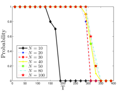
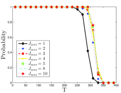
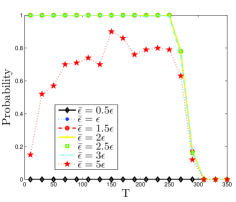
First we study the influence of the parameters in the PDASC algorithm on the exact recovery probability. To this end, we fix $\Psi$ to be a $500\times 1000$ random Gaussian matrix, and $\sigma=\mbox{1e-2}$. All the results are computed based on 100 independent realizations of the problem setup. To this end, we consider the following three settings:

1. $J_{max}=5$, and varying $N$; see Fig. 1(a).

2. $N=100$, and varying $J_{max}$; see Fig. 1(b).

3. $N=100$, $J_{max}=5$, and an approximate noise level $\bar{\epsilon}$; see Fig. 1(c).

We observe that the influence of the parameters $N$ and $J_{max}$ is very mild on the exact support recovery probability. In particular, a reasonably small value for these parameters (e.g. $N=50$, $J_{max}=1$) is sufficient for accurately recovering the exact active set $A^{*}$. Unsurprisingly, a very small value of $N$ can degrade the accuracy of active set recovery greatly, due to insufficient resolution of the solution path. In practice, the exact noise level $\epsilon$ is not always available, and often only a rough estimate $\bar{\epsilon}$ is provided. The use of the estimate $\bar{\epsilon}$ in place of the exact one $\epsilon$ in Algorithm 1 may sacrifice the recovery probability. Hence it is important to study the sensitivity of Algorithm 1 with respect to the variation of the parameter $\epsilon$. We observe from Fig. 1(c) that the parameter $\epsilon$ does not affect the recovery probability much, unless the estimate $\bar{\epsilon}$ is grossly erroneous.

(a) $N$	(b) $J_{max}$
(c) $\epsilon$

Figure 1: The influence of the algorithmic parameters ($N$, $J_{max}$ and $\epsilon$) on the exact recovery probability.

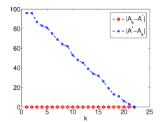
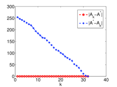
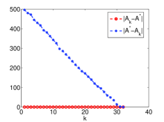
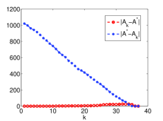
To gain further insight into the PDASC algorithm, in Fig. 2, we show the evolution of the active set (for simplicity let $A_{k}=A(\lambda_{k})$) . It is observed that the active set $A_{k}$ can generally move both “inside” and “outside” of the true active set $A^{*}$. This is in sharp contrast to the OMP, where the size of the active set is monotone during the iteration. The flexible change in the active set might be essential for the efficiency of the algorithm. This observation is valid for random Gaussian, random Bernoulli and partial DCT sensing matrices.

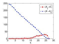(a) random Gaussian, $T=100$	(b) random Gaussian, $T=250$
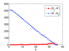(c) random Bernoulli, $T=2^{8}$	(d) random Bernoulli, $T=2^{9}$
(e) partial DCT, $T=2^{9}$	(f) partial DCT, $T=2^{10}$

Figure 2: Numerical results for random Gaussian (top row, $R=100$, $n=500$, $p=1000$, $\sigma=\mbox{1e-3}$), random Bernoulli (middle row, $R=1000$, $n=2^{10}$, $p=2^{12}$, $\sigma=\mbox{1e-3}$) and partial DCT (bottom row, $R=1000$, $n=2^{11}$, $p=2^{13}$, $\sigma=\mbox{1e-3}$) sensing matrix. The parameters $N$ and $J_{max}$ are set to $N=50$ and $J_{max}=1$, respectively.

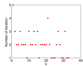
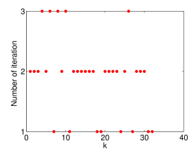
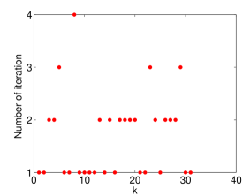
For each $\lambda_{k}$, with $x({\lambda_{k-1}})$ ($x({\lambda_{0}})=0$) as the initial guess, the PDASC generally reaches convergence within a few iterations, cf. Fig. 3, which is observed for random Gaussian, random Bernoulli and partial DCT sensing matrices. This is attributed to the local superlinear convergence of the PDAS algorithm. Hence, when coupled with the continuation strategy, the PDASC procedure is very efficient.

(a) Random Gaussian	(b) Random Bernoulli
(c) Partial DCT

Figure 3: Number of iterations of PDASC at each $\lambda_{k}$ for random Gaussian (top left with $R=1000$, $n=500$, $p=1000$, $T=200$, $\sigma=\mbox{1e-3}$), random Bernoulli (top right with $R=1000$, $n=2^{10}$, $p=2^{12}$, $T=2^{8}$, $\sigma=\mbox{1e-3}$) and partial DCT (bottom with $R=1000$, $n=2^{11}$, $p=2^{13}$, $T=2^{8}$, $\sigma=\mbox{1e-3}$) sensing matrix. The parameters $N$ and $J_{max}$ are set to $N=50$ and $J_{max}=5$, respectively.

4.2 Comparison with existing algorithms

In this part, we compare Algorithm 1 with six state-of-the-art algorithms in the compressive sensing literature, including orthogonal matching pursuit (OMP) [31], greedy gradient pursuit (GreedyGP) [5], accelerated iterative hard thresholding (AIHT) [3], hard thresholding pursuit (HTP) [16], compressive sampling matching pursuit (CoSaMP) [25] and homotopy algorithm [14, 29].

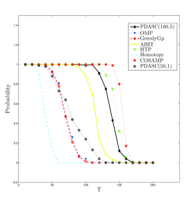
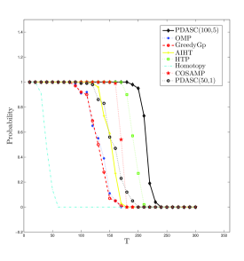
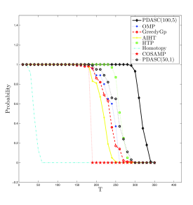
First, we consider the exact support recovery probability, i.e., the percentage of the reconstructions whose support agrees with the true active set $A^{*}$. To this end, we fix the sensing matrix $\Psi$ as a $500\times 1000$ random Gaussian matrix, $\sigma=\mbox{1e-3}$, $(N,J_{max})=(100,5)$ or $(50,1)$, and all results are computed from $100$ independent realizations of the problem setup. Since the different dynamical range may give different results, we take $R=1$, $10$, 1e3, 1e5 as four exemplary values. The numerical results are summarized in Fig. 4. We observe that when the dynamical range $R$ is not very small, the proposed PDASC algorithm with $(N,J_{max})=(100,5)$ has a better exact support recovery probability, and that with the choice $(N,J_{max})$ is largely comparable with other algorithms.

(a) $R=1$	(b) $R=10$
(c) $R=10^{3}$	(d) $R=10^{5}$

Figure 4: The exact support recovery probability for four different dynamical ranges: $R=1,\ 10,\ 10^{3}$, and $10^{5}$.

To further illustrate the accuracy and efficiency of the proposed PDASC algorithm, we compare it with other greedy methods in terms of CPU time and reconstruction error. To this end, we fix $\sigma=\mbox{1e-2}$, $(N,J_{max})=(100,5)$ or $(50,1)$. The numerical results for random Gaussian, random Bernoulli and partial DCT sensing matrices with different parameter tuples $(R,n,p,T)$ are shown in Tables 4.1-4.3, respectively. The results in the tables are computed from 10 independent realizations of the problem setup. It is observed that the PDASC algorithm yields reconstructions that are comparable with that by other methods, but usually with less computing time. Further, we observe that it scales better with the problem size than other algorithms.

Table 4.1: Numerical results (CPU time and errors) for medium-scale problems, with random Gaussian sensing matrix $\Psi$, of size $p=10000,\ 15000,\ 20000,\ 25000,\ 30000$, $n=\lfloor p/4\rfloor$, $T=\lfloor n/3\rfloor$. The dynamical range $R$ is $R=1000$, and the noise variance $\sigma$ is $\sigma=\mbox{1e-2}$.

$p$	method	time(s)	Relative $\ell^{2}$ error	Absolute $\ell^{\infty}$ error
	PDASC(50,1)	1.94	4.24e-5	3.91e-2
	PDASC(100,5)	6.41	4.49e-5	3.81e-2
$10000$	OMP	17.4	4.24e-5	3.91e-2
	GreedyGP	17.9	7.50e-5	1.35e-1
	AIHT	4.62	4.24e-5	3.91e-2
	HTP	1.69	4.24e-5	3.91e-2
	CoSaMP	10.4	1.21e-1	8.87e+1
	PDASC(50,1)	4.17	4.32e-5	4.60e-2
	PDASC(100,5)	17.4	4.60e-5	4.55e-2
$15000$	OMP	56.8	4.32e-5	4.60e-2
	GreedyGP	61.4	6.36e-5	1.17e-1
	AIHT	9.88	4.32e-5	4.60e-2
	HTP	4.52	4.32e-5	4.60e-2
	CoSaMP	32.4	8.93e-2	7.24e+1
	PDASC(50,1)	8.14	4.50e-5	4.68e-2
	PDASC(100,5)	34.8	4.56e-5	4.34e-2
$20000$	OMP	134	4.50e-5	4.68e-2
	GreedyGP	141	6.12e-5	1.11e-1
	AIHT	18.4	4.50e-5	4.67e-2
	HTP	9.51	4.50e-5	4.68e-2
	CoSaMP	79.7	1.12e-1	8.03e+1
	PDASC(50,1)	13.7	4.47e-5	4.03e-2
	PDASC(100,5)	62.3	4.55e-5	4.61e-2
$25000$	OMP	260	4.47e-5	4.03e-2
	GreedyGP	275	6.19e-5	1.35e-1
	AIHT	26.8	4.47e-5	4.03e-2
	HTP	19.6	4.47e-5	4.03e-2
	CoSaMP	150	1.07e-1	7.96e+1
	PDASC(50,1)	21.1	4.52e-5	4.90e-2
	PDASC(100,5)	95.9	4.53e-5	4.53e-2
$30000$	OMP	445	4.52e-5	4.90e-2
	GreedyGP	475	5.57e-5	1.02e-1
	AIHT	40.3	4.52e-5	4.90e-2
	HTP	29.8	4.52e-5	4.90e-2
	CoSaMP	251	9.00e-2	6.48e+1

Table 4.2: Numerical results (CPU time and errors) for medium-scale problems, with random Bernoulli sensing matrix $\Psi$, of size $p=10000,\ 15000,\ 20000,\ 25000,\ 30000$, $n=\lfloor p/4\rfloor$, $T=\lfloor n/4\rfloor$. The dynamical range $R$ is $R=10$, and the noise variance $\sigma$ is $\sigma=\mbox{1e-2}$.

$p$	method	time(s)	Relative $\ell^{2}$ error	Absolute $\ell^{\infty}$ error
	PDASC(50,1)	0.62	2.33e-3	3.66e-2
	PDASC(100,5)	2.56	2.50e-3	3.82e-2
$10000$	OMP	9.92	2.33e-3	3.70e-2
	GreedyGP	11.8	1.80e-2	1.02e+0
	AIHT	3.50	2.31e-3	3.64e-2
	HTP	0.90	2.31e-3	3.64e-2
	CoSaMP	4.50	4.68e-3	6.71e-2
	PDASC(50,1)	1.41	2.39e-3	3.62e-2
	PDASC(100,5)	6.44	2.50e-3	4.11e-2
$15000$	OMP	33.4	2.40e-3	3.63e-2
	GreedyGP	40.1	1.86e-2	1.03e+0
	AIHT	7.19	2.39e-3	3.62e-2
	HTP	2.27	2.39e-3	3.62e-2
	CoSaMP	13.6	5.06e-3	8.07e-2
	PDASC(50,1)	2.67	2.52e-3	4.21e-2
	PDASC(100,5)	12.7	2.50e-3	3.97e-2
$20000$	OMP	78.5	2.53e-3	4.18e-2
	GreedyGP	94.9	1.55e-2	1.02e+0
	AIHT	12.8	2.52e-3	4.20e-2
	HTP	4.25	2.52e-3	4.20e-2
	CoSaMP	30.1	4.99e-3	7.69e-2
	PDASC(50,1)	4.51	2.49e-3	4.16e-2
	PDASC(100,5)	21.7	2.50e-3	3.99e-2
$25000$	OMP	152.	2.50e-3	4.21e-2
	GreedyGP	185.	2.14e-2	1.07e+0
	AIHT	23.9	2.49e-3	4.17e-2
	HTP	7.78	2.49e-3	4.17e-2
	CoSaMP	58.4	5.04e-3	8.13e-2
	PDASC(50,1)	6.90	2.45e-3	8.67e-2
	PDASC(100,5)	34.7	2.50e-3	4.18e-2
$30000$	OMP	264.	2.46e-3	1.01e-2
	GreedyGP	324.	1.72e-2	1.01e+0
	AIHT	24.7	2.45e-3	8.47e-2
	HTP	10.7	2.45e-3	8.46e-2
	CoSaMP	93.3	4.97e-3	3.63e+1

Table 4.3: Numerical results (CPU time and errors) for large-scale problems, with partial DCT sensing matrix $\Psi$, of size $p=2^{13}$, $2^{14}$, $2^{15}$, $2^{16}$, $2^{17}$, $n=\lfloor p/4\rfloor$, $T=\lfloor n/3\rfloor$. The dynamical range $R$ is $R=100$, and the noise variance $\sigma$ is $\sigma=\mbox{1e-2}$.

$p$	method	time(s)	Relative $\ell^{2}$ error	Absolute $\ell^{\infty}$ error
	PDASC(50,1)	0.31	7.11e-4	7.78e-2
	PDASC(100,5)	1.51	7.08e-4	7.93e-2
$p=2^{13}$	OMP	2.26	7.06e-4	7.75e-2
	GreedyGP	0.74	1.07e-3	1.79e-1
	AIHT	0.35	7.06e-4	7.75e-2
	HTP	0.57	7.06e-4	7.75e-2
	CoSaMP	0.55	3.74e-1	3.10e+1
	PDASC(50,1)	0.48	7.05e-4	7.43e-2
	PDASC(100,5)	3.30	6.95e-4	8.49e-2
$2^{14}$	OMP	11.3	7.00e-4	7.49e-2
	GreedyGP	2.52	1.21e-3	5.95e-1
	AIHT	0.48	7.01e-4	7.53e-2
	HTP	0.95	7.01e-4	7.53e-2
	CoSaMP	0.87	3.52e-1	2.95e+1
	PDASC(50,1)	0.85	8.68e-4	5.52e-1
	PDASC(100,5)	6.59	7.42e-4	1.74e-1
$2^{15}$	OMP	65.6	9.94e-4	1.00e-2
	GreedyGP	10.0	8.08e-4	1.95e-1
	AIHT	0.90	7.15e-4	8.27e-2
	HTP	1.73	7.15e-4	8.27e-2
	CoSaMP	1.55	3.90e-1	4.11e+1
	PDASC(50,1)	1.60	7.33e-4	8.67e-2
	PDASC(100,5)	13.2	7.07e-4	8.81e-2
$2^{16}$	OMP	410	1.13e-3	1.01e+0
	GreedyGP	35.8	1.00e-3	1.01e+0
	AIHT	2.00	7.28e-4	8.47e-2
	HTP	3.59	7.28e-4	8.46e-2
	CoSaMP	2.75	3.74e-1	3.63e+1
	PDASC(50,1)	4.37	7.17e-4	1.00e-1
	PDASC(100,5)	37.1	7.13e-4	9.86e-2
$2^{17}$	OMP	3.11e+3	1.11e-3	1.02e+0
	GreedyGP	199	7.96e-4	5.98e-1
	AIHT	4.90	7.14e-4	1.00e-1
	HTP	9.03	7.14e-4	1.00e-1
	CoSaMP	7.70	3.90e-1	3.90e+1

Lastly, we consider one-dimensional signals and two-dimensional images. In this case the explicit form of the sensing matrix $\Psi$ may be not available, hence the least-squares step (for updating the primal variable) at line 7 of Algorithm 1 can only be solved by an iterative method. We employ the conjugate gradient (CG) method to solve the least-squares problem inexactly. The initial guess for the CG method for the $\lambda_{k}$-problem is the solution $x(\lambda_{k-1})$, and the stopping criterion for the CG method is as follows: either the number of CG iterations is greater than 2 or the residual is below a given tolerance $\mbox{1e-5}\epsilon$.

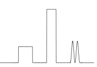
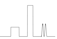
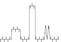
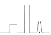
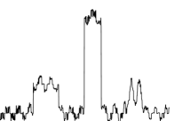
For the one-dimensional signal, the sampling matrix $\Psi$ is of size $665\times 1024$, and it consists of applying a partial FFT and an inverse wavelet transform, and the signal under wavelet transformation has $247$ nonzero entries and $\sigma=\mbox{1e-4}$, $N=50$, $J_{\max}=1$. The results are shown in Fig. 5 and Table 4.4. The reconstructions by all the methods, except the AIHT and CoSaMP, are visually very appealing and in excellent agreement with the exact solution. The reconstructions by the AIHT and CoSaMP suffer from pronounced oscillations. This is further confirmed by the PSNR values which is defined as

$$\textit{PSNR}=10\cdot\log\frac{V^{2}}{MSE}$$

where $V$ is the maximum absolute value of the reconstruction and the true solution, and $MSE$ is the mean squared error of the reconstruction, cf. Table 4.4.

For the two-dimensional MRI image, the sampling matrix $\Psi$ amounts to a partial FFT and an inverse wavelet transform of size $1657\times 4096$. The image under wavelet transformation has $792$ nonzero entries and $\sigma=\mbox{1e-4}$, $N=50$, and $J_{\max}=1$. The numerical results are shown in Fig. 6 and Table 4.5. The observation for the one-dimensional signal remains largely valid: except the CoSaMP, all other methods can yield almost identical reconstructions within similar computational efforts. Therefore, the proposed PDASC algorithm is competitive with state-of-the-art algorithms.

(a) PDASC	(b) OMP
(c) GreedyGP	(d) AIHT
(e) HTP	(f) CoSaMP

Figure 5: Reconstruction results of 1 dimension signal.

(a) PDASC	(b) OMP
(c) GreedyGP	(d) AIHT
(e) HTP	(f) CoSaMP

Figure 6: Reconstruction results of two-dimensional phantom images.

Table 4.4: One-dimensional signal: $n=665$, $p=1024$, $T=247$, $\sigma=\mbox{1e-4}$.

method	CPU time	PSNR
PDASC	0.49	53
OMP	1.45	49
GreedyGp	0.76	49
AIHT	0.58	34
HTP	0.40	51
CoSaMP	0.91	26

Table 4.5: Two-dimensional image, $n=1657$, $p=4096$, $T=792$, $\sigma=\mbox{1e-4}$.

method	CPU time	PSNR
PDASC	0.71	81
OMP	6.82	83
GreedyGP	2.93	74
AIHT	0.56	74
HTP	0.57	82
CoSaMP	1.46	20

5 Conclusion

We have developed an efficient and accurate primal-dual active set with continuation algorithm for the $\ell^{0}$ penalized least-squares problem arising in compressive sensing. It combines the fast local convergence of the active set technique and the globalizing property of the continuation technique. The global finite step convergence of the algorithm was established under the mutual incoherence property or restricted isometry property on the sensing matrix. Our extensive numerical results indicate that the proposed algorithm is competitive in comparison with state-of-the-art algorithms in terms of efficiency, accuracy and exact recovery probability, without a knowledge of the exact sparsity level.

References

- [1] H. Attouch, J. Bolte, and B. F. Svaiter. Convergence of descent methods for semi-algebraic and tame problems: proximal algorithms, forward-backward splitting, and regularized Gauss-Seidel methods. Math. Program., 137(1-2, Ser. A):91–129, 2013.
- [2] F. Bach, R. Jenatton, J. Mairal, and G. Obozinski. Optimization with Sparsity-Inducing Penalties. Found. Trend. Mach. Learn., 4(1):1–106, 2012.
- [3] T. Blumensath. Accelerated iterative hard thresholding. Sig. Proc., 92(3):752–756, 2012.
- [4] T. Blumensath and M. E. Davies. Iterative hard thresholding for compressed sensing. Appl. Comput. Harmon. Anal., 27(3):265–274, 2009.
- [5] T. Blumensath and M. E. Davies. Stagewise weak gradient pursuits. IEEE Trans. Signal Process., 57(11):4333–4346, 2009.
- [6] T. T. Cai and L. Wang. Orthogonal matching pursuit for sparse signal recovery with noise. IEEE Trans. Inform. Theory, 57(7):4680–4688, 2011.
- [7] E. J. Candès, J. Romberg, and T. Tao. Robust uncertainty principles: exact signal reconstruction from highly incomplete frequency information. IEEE Trans. Inform. Theory, 52(2):489–509, 2006.
- [8] E. J. Candes and T. Tao. Decoding by linear programming. IEEE Trans. Inf. Theory, 51(12):4203–4215, 2005.
- [9] S. S. Chen, D. L. Donoho, and M. A. Saunders. Atomic decomposition by basis pursuit. SIAM J. Sci. Comput., 20(1):33–61, 1998.
- [10] P. Combettes and J. Pesquet. Proximal splitting methods in signal processing. In H. H. Bauschke, R. S. Burachik, P. L. Combettes, V. Elser, D. R. Luke, and H. Wolkowicz, editors, Fixed-Point Algorithms for Inverse Problems in Science and Engineering, pages 185–212. Springer, Berlin, 2011.
- [11] W. Dai and O. Milenkovic. Subspace pursuit for compressive sensing signal reconstruction. IEEE Trans. Inform. Theory, 55(5):2230–2249, 2009.
- [12] D. L. Donoho. Compressed sensing. IEEE Trans. Inform. Theory, 52(4):1289–1306, 2006.
- [13] D. L. Donoho and X. Huo. Uncertainty principles and ideal atomic decomposition. IEEE Trans. Inf. Theory, 47(7):2845–2862, 2001.
- [14] D. L. Donoho and Y. Tsaig. Fast solution of -norm minimization problems when the solution may be sparse. IEEE Trans. Inf. Theory, 54(11):4789–4812, 2008.
- [15] D. L. Donoho, Y. Tsaig, I. Drori, and J.-L. Starck. Sparse solution of underdetermined systems of linear equations by stagewise orthogonal matching pursuit. IEEE Trans. Inform. Theory, 58(2):1094–1121, 2012.
- [16] S. Foucart. Hard thresholding pursuit: an algorithm for compressive sensing. SIAM J. Numer. Anal., 49(6):2543–2563, 2011.
- [17] S. Huang and J. Zhu. Recovery of sparse signals using OMP and its variants: convergence analysis based on RIP. Inverse Problems, 27(3):035003, 14 pp., 2011.
- [18] K. Ito and B. Jin. Inverse Problems: Tikhonov Theory and Algorithms. World Scientific, Singapore, 2014.
- [19] K. Ito, B. Jin, and T. Takeuchi. A regularization parameter for nonsmooth Tikhonov regularization. SIAM J. Sci. Comput., 33(3):1415–1438, 2011.
- [20] K. Ito and K. Kunisch. Lagrange Multiplier Approach to Variational Problems and Applications, volume 15 of Advances in Design and Control. SIAM, Philadelphia, PA, 2008.
- [21] K. Ito and K. Kunisch. A variational approach to sparsity optimization based on Lagrange multiplier theory. Inverse Problems, 30(1):015001, 23 pp, 2014.
- [22] Y. Jiao, B. Jin, and X. Lu. A primal dual active set algorithm for a class of nonconvex sparsity optimization. preprint, arXiv:1310.1147, 2013.
- [23] Z. Lu and Y. Zhang. Sparse approximation via penalty decomposition methods. SIAM J. Optim., 23(4):2448–2478, 2013.
- [24] Q. Mo and Y. Shen. A remark on the restricted isometry property in orthogonal matching pursuit. IEEE Trans. Inform. Theory, 58(6):3654–3656, 2012.
- [25] D. Needell and J. A. Tropp. CoSaMP: iterative signal recovery from incomplete and inaccurate samples. Appl. Comput. Harmon. Anal., 26(3):301–321, 2009.
- [26] D. Needell and R. Vershynin. Uniform uncertainty principle and signal recovery via regularized orthogonal matching pursuit. Found. Comput. Math., 9(3):317–334, 2009.
- [27] M. Nikolova. Description of the minimizers of least squares regularized with -norm. Uniqueness of the global minimizer. SIAM J. Imaging Sci., 6(2):904–937, 2013.
- [28] M. Nikolova. Relationship between the optimal solutions of least squares regularized with -norm and constrained by k-sparsity. preprint, 2014.
- [29] M. R. Osborne, B. Presnell, and B. A. Turlach. A new approach to variable selection in least squares problems. IMA J. Numer. Anal., 20(3):389–403, 2000.
- [30] N. Parikh and S. Boyd. Proximal algorithms. Found. Trends Optim., 1(3):123–231, 2014.
- [31] Y. Pati, R. Rezaiifar, and P. Krishnaprasad. Orthogonal matching pursuit: Recursive function approximation with applications to wavelet decomposition. In Signals, Systems and Computers, 1993. 1993 Conference Record of The 27th Asilomar Conference on, volume 1, pages 40–44. IEEE.
- [32] M. C. Robini and I. E. Magnin. Optimization by stochastic continuation. SIAM J. Imaging Sci., 3(4):1096–1121, 2010.
- [33] M. C. Robini and P.-J. Reissman. From simulated annealing to stochastic continuation: a new trend in combinatorial optimization. J. Global Optim., 56(1):185–215, 2013.
- [34] R. Tibshirani. Regression shrinkage and selection via the lasso. J. Roy. Statist. Soc. Ser. B, 58(1):267–288, 1996.
- [35] J. Tropp and S. Wright. Computational methods for sparse solution of linear inverse problems. Proc. IEEE, 98(6):948–958, 2010.
- [36] J. A. Tropp. Greed is good: algorithmics results for sparse approximation. IEEE Trans. Inf. Theory, 50(2):2231–2242, 2004.
- [37] P. Tseng. Convergence of a block coordinate descent method for nondifferentiable minimization. J. Optim. Theory Appl., 109(3):475–494, 2001.
- [38] T. Zhang. Sparse recovery with orthogonal matching pursuit under RIP. IEEE Trans. Inform. Theory, 57(9):6215–6221, 2011.