Scaling hypothesis for the Euclidean bipartite matching problem

S. Caracciolo Dipartimento di Fisica, Università degli Studi di Milano and INFN, via Celoria, I-20133 Milano, Italy    C. Lucibello Dipartimento di Fisica, Università “La Sapienza”, P.le A. Moro 2, I-00185, Rome, Italy    G. Parisi Dipartimento di Fisica, INFN – Sezione di Roma1, CNR-IPCF UOS Roma Kerberos, Università “La Sapienza”, P.le A. Moro 2, I-00185, Rome, Italy    G. Sicuro Dipartimento di Fisica “Enrico Fermi”, Università di Pisa, and INFN – Sezione di Pisa, Largo Bruno Pontecorvo 3, I-56127, Pisa, Italy
Abstract

We propose a simple yet very predictive form, based on a Poisson’s equation, for the functional dependence of the cost from the density of points in the Euclidean bipartite matching problem. This leads, for quadratic costs, to the analytic prediction of the large N𝑁N limit of the average cost in dimension d=1,2𝑑12d=1,2 and of the subleading correction in higher dimension. A non-trivial scaling exponent, γd=d2dsubscript𝛾𝑑𝑑2𝑑\gamma_{d}=\frac{d-2}{d}, which differs from the monopartite’s one, is found for the subleading correction. We argue that the same scaling holds true for a generic cost exponent in dimension d>2𝑑2d>2.

I Introduction and Main Results

The matching problem is a combinatorial optimization problem that has drawn the attention of both the computer science Kuhn (1955); Munkres (1957); Papadimitriou and Steiglitz (1998); Edmonds (1965); Bayati et al. (2008) and the statistical physics Mézard and Parisi (1985, 1986); Martin et al. (2001); Parisi and Ratiéville (2002) communities for many decades. Even in its most general formulation, the problem belongs to the P𝑃P computational complexity class, and many famous algorithms have been developed to solve it efficiently Kuhn (1955); Munkres (1957).

In this paper we focus on a restricted version of the problem, the complete bipartite matching problem, also known as the assignment problem, that, by itself, has a long standing tradition among the scholars Mézard and Parisi (1985); Papadimitriou and Steiglitz (1998); Mézard and Montanari (2009): in this problem we have two sets of the same cardinality N𝑁N (let us call them \mathcal{R} and \mathcal{B}) and we want to find a one-to-one correspondence between the elements of \mathcal{R} and the elements of \mathcal{B} in such a way that all the elements are paired and a certain global function of this matching (called the cost function) is minimized. An instance of the assignment problem is a N×N𝑁𝑁N\times N matrix w𝑤w: each element wijsubscript𝑤𝑖𝑗w_{ij} gives the partial cost of the assignment of the element i𝑖i\in\mathcal{B} to the element j𝑗j\in\mathcal{R}. From a combinatorial point of view, an assignment is a permutation π𝒮N𝜋subscript𝒮𝑁\pi\in\mathcal{S}_{N}, where 𝒮Nsubscript𝒮𝑁\mathcal{S}_{N} is the set of permutations of N𝑁N elements. Its cost is defined by

EN[π;w]=1Ni=1Nwiπ(i).subscript𝐸𝑁𝜋𝑤1𝑁superscriptsubscript𝑖1𝑁subscript𝑤𝑖𝜋𝑖E_{N}[\pi;w]=\frac{1}{N}\sum_{i=1}^{N}w_{i\pi(i)}. (1)

The optimization problem consists in finding the optimal assignment πsuperscript𝜋\pi^{*}, i.e., the assignment πsuperscript𝜋\pi^{*} that satisfies the property EN[π,w]=minπ𝒮NEN[π;w]subscript𝐸𝑁superscript𝜋𝑤subscript𝜋subscript𝒮𝑁subscript𝐸𝑁𝜋𝑤E_{N}[\pi^{*},w]=\min_{\pi\in\mathcal{S}_{N}}E_{N}[\pi;w].

Some interesting questions arise when random instances of the problem are considered, that is, when the elements of the cost matrix w𝑤w are chosen according to a certain probability law. We will discuss the properties of the system for different choices of the disorder, i.e., of the distribution of w𝑤w. Let us consider the average optimal cost EN=EN[π;w]¯subscript𝐸𝑁¯subscript𝐸𝑁superscript𝜋𝑤E_{N}=\overline{E_{N}[\pi^{*};w]}, where ¯¯\overline{\,\bullet\,} denotes the expectation over the instances w𝑤w of the problem. If we choose the problem ensemble such that the matrix elements wijsubscript𝑤𝑖𝑗w_{ij} are i.i.d. random variables, we obtain the so-called random assignment problem. This version of the problem was largely investigated in a set of papers in which both the distribution of the optimal weights in the large N𝑁N limit Mézard and Parisi (1985); Aldous (2001) and the finite sizes corrections (Parisi and Ratiéville, 2002) were derived using different approaches. In this context, the celebrated replica approach, directly borrowed from the theory of spin glasses and disordered systems, proved to be an excellent tool to investigate the properties of these random optimization problems, and led to the celebrated formula limNEN=π26subscript𝑁subscript𝐸𝑁superscript𝜋26\lim_{N\to\infty}E_{N}=\frac{\pi^{2}}{6} under certain assumptions over the distribution of wijsubscript𝑤𝑖𝑗w_{ij} Mézard and Parisi (1985). Quite interestingly the average optimal cost ENsubscript𝐸𝑁E_{N} for the random assignment problem is known exactly for every value of N𝑁N. It is given by the simple formula EN=k=1N1k2subscript𝐸𝑁superscriptsubscript𝑘1𝑁1superscript𝑘2E_{N}=\sum_{k=1}^{N}\frac{1}{k^{2}}, as has been first conjectured in Parisi1998 and independently proven in Refs. Linusson2004 and Nair2003.

From an analytical point of view, a much more difficult problem arises when the elements of the cost matrix w𝑤w are correlated. This is indeed the case of the Euclidean assignment problem, also known as Euclidean bipartite matching problem (Ebmp). The Ebmp is an assignment problem in which a set of N𝑁N “blue” points ={𝐛i}i=1Nsuperscriptsubscriptsubscript𝐛𝑖𝑖1𝑁\mathcal{B}=\{\mathbf{b}_{i}\}_{i=1}^{N} and a set of N𝑁N “red” points ={𝐫i}i=1Nsuperscriptsubscriptsubscript𝐫𝑖𝑖1𝑁\mathcal{R}=\{\mathbf{r}_{i}\}_{i=1}^{N} are given on the hypercube [0,1]dsuperscript01𝑑[0,1]^{d}. Each point is supposed to be generated independently and uniformly at random in the hypercube. Periodic boundary conditions are imposed (in other words, to avoid scaling corrections due to border effects, we consider the sets of points on the torus 𝖳dd/dsuperscript𝖳𝑑superscript𝑑superscript𝑑\mathsf{T}^{d}\equiv\mathbb{R}^{d}/\mathbb{Z}^{d}). The cost of the matching between two points is then given by a function of their distance on the torus. We will generalize the Euclidean flat distance on the torus to a family of functions characterized by a cost exponent p𝑝p, assuming that

wij=𝐛i𝐫jp,subscript𝑤𝑖𝑗superscriptnormsubscript𝐛𝑖subscript𝐫𝑗𝑝w_{ij}={\left\|\mathbf{b}_{i}-\mathbf{r}_{j}\right\|}^{p}, (2)

where 𝐛i𝐫jk=1d(min{|bikrjk|,1|bikrjk|})2normsubscript𝐛𝑖subscript𝐫𝑗superscriptsubscript𝑘1𝑑superscriptsubscriptsuperscript𝑏𝑘𝑖superscriptsubscript𝑟𝑗𝑘1subscriptsuperscript𝑏𝑘𝑖superscriptsubscript𝑟𝑗𝑘2{\left\|\mathbf{b}_{i}-\mathbf{r}_{j}\right\|}\coloneqq\sqrt{\sum_{k=1}^{d}\left(\min\left\{{\left|b^{k}_{i}-r_{j}^{k}\right|},1-{\left|b^{k}_{i}-r_{j}^{k}\right|}\right\}\right)^{2}} is the Euclidean norm on the torus. Due to the underlying Euclidean structure, the elements of w𝑤w present very strong correlations. We shall denote with EN(p)(d)subscriptsuperscript𝐸𝑝𝑁𝑑E^{(p)}_{N}(d) the average cost of the optimal assignment between N𝑁N red points and N𝑁N blue points on 𝖳dsuperscript𝖳𝑑\mathsf{T}^{d} with cost exponent p𝑝p, that is

EN(p)(d)EN(p)[π;{𝐫i,𝐛i}]¯,subscriptsuperscript𝐸𝑝𝑁𝑑¯subscriptsuperscript𝐸𝑝𝑁superscript𝜋subscript𝐫𝑖subscript𝐛𝑖E^{(p)}_{N}(d)\equiv\overline{E^{(p)}_{N}[\pi^{*};\{\mathbf{r}_{i},\mathbf{b}_{i}\}]}, (3)

where the average is intended over the positions of the points and πsuperscript𝜋\pi^{*} is the optimal permutation. In the following we will sometimes drop the dependence on p𝑝p and on d𝑑d of the optimal cost, and write simply ENsubscript𝐸𝑁E_{N}.

The scaling behaviour of the leading order of the optimal cost is well known for p>1𝑝1p>1 and all values of d𝑑d and has been confirmed also by the investigations conducted by means of statistical physics methods. In fact, from a simple heuristic argument Mézard and Parisi (1988), we expect that, given a red point, the nearest blue points can be found approximately in a volume of order O(1N)𝑂1𝑁O\left(\frac{1}{N}\right) around it: their distances from the red point is, for this reason, of order N1dsuperscript𝑁1𝑑N^{-\frac{1}{d}}. Supposing that each red point is matched to one of its nearest blue points, the expected total cost scales as EN=O(Npd)subscript𝐸𝑁𝑂superscript𝑁𝑝𝑑E_{N}=O\left(N^{-\frac{p}{d}}\right) for large N𝑁N. It turns out that this asymptotic estimation is correct only for d3𝑑3d\geq 3 as it can be rigorously proved Talagrand (1992). In a fundamental paper on this subject, published in 1984, Ajtai et al. (1984) proved that for d=2𝑑2d=2 a logarithmic correction appears, EN=O((lnNN)p2)subscript𝐸𝑁𝑂superscript𝑁𝑁𝑝2E_{N}=O\left(\left(\frac{\ln N}{N}\right)^{\frac{p}{2}}\right). In dimension d=1𝑑1d=1 instead, the divergence from the expected result is even greater, in fact it is informally known to the literature Ajtai et al. (1984); Boniolo2014 (even if to our knowledge nowhere formally stated), that EN=O(Np2)subscript𝐸𝑁𝑂superscript𝑁𝑝2E_{N}=O\left(N^{-\frac{p}{2}}\right) in this case. We can resume the state of the art of knowledge regarding the asymptotic behaviour of the average optimal cost in the Ebmp, with the following formula:

βN(p)(d)EN(p)(d)Npd={O(Np2)d=1,O((logN)p2)d=2,ed(p)+O(Nγd)d>2.subscriptsuperscript𝛽𝑝𝑁𝑑subscriptsuperscript𝐸𝑝𝑁𝑑superscript𝑁𝑝𝑑cases𝑂superscript𝑁𝑝2𝑑1𝑂superscript𝑁𝑝2𝑑2superscriptsubscript𝑒𝑑𝑝𝑂superscript𝑁subscript𝛾𝑑𝑑2\beta^{(p)}_{N}(d)\equiv\frac{E^{(p)}_{N}(d)}{N^{-\frac{p}{d}}}=\begin{cases}O(N^{\frac{p}{2}})&d=1,\\ O\left((\log N)^{\frac{p}{2}}\right)&d=2,\\ e_{d}^{(p)}+O(N^{-\gamma_{d}})&d>2.\end{cases} (4)

The determination of the exponents γdsubscript𝛾𝑑\gamma_{d} is one of the contributions of the present paper and it will be discussed in the following. The coefficients ed(p)superscriptsubscript𝑒𝑑𝑝e_{d}^{(p)} are not known to the literature and could not be derived using our approach either, even though we give accurate numerical estimates in Table 2. The rescaled average optimal cost, βN(p)(d)subscriptsuperscript𝛽𝑝𝑁𝑑\beta^{(p)}_{N}(d), is what a physicist would call the intensive energy, and will be used in the rest of the paper. As with ENsubscript𝐸𝑁E_{N}, we will sometimes drop the p𝑝p and d𝑑d dependence from it and write simply βNsubscript𝛽𝑁\beta_{N}.

The scenario depicted in Eq. (4) has to be compared with the one arising in the Euclidean monopartite matching problem (Emmp). Mézard and Parisi (1988) studied analytically this problem considering the correlations among the costs as perturbations around the case with random independent entries wijsubscript𝑤𝑖𝑗w_{ij}. In the Emmp there is a unique set of 2N2𝑁2N points to be matched among themselves. It has been proven Steele (1997); Yukich (1998) that, in the Emmp, the rescaled average optimal cost βN(p)(d)subscriptsuperscript𝛽𝑝𝑁𝑑\beta^{(p)}_{N}(d) has a finite limit and is a self-averaging quantity in every dimension d𝑑d. The odd behaviour noticed in the bipartite case in low dimensions is due to the presence of differences, in small regions of space, between the number of red and blue points, that imply the presence of “long distance” pairings and the failure of arguments based on subadditivity Houdayer et al. (1998). Obviously, in the monoportite cases such problems do not exist, since a partial matching between the points in an arbitrary subregion of [0,1]dsuperscript01𝑑[0,1]^{d} leaves only one point at most unpaired.

Moreover numeric and analytic arguments Houdayer et al. (1998) show that in the Emmp the first subleading correction to the large N𝑁N limit of βNsubscript𝛽𝑁\beta_{N} is of order O(N1)𝑂superscript𝑁1O(N^{-1}) in any dimension. This assumptions though was also been improperly used in the Ebmp to numerically extrapolate the value ed(p)=limNβN(p)(d)superscriptsubscript𝑒𝑑𝑝subscript𝑁subscriptsuperscript𝛽𝑝𝑁𝑑e_{d}^{(p)}=\lim_{N\to\infty}\beta^{(p)}_{N}(d) for d>2𝑑2d>2 in the case of flat distances Houdayer et al. (1998) (i.e. p=1𝑝1p=1). This led to some inaccurate estimations of ed(1)superscriptsubscript𝑒𝑑1e_{d}^{(1)} that we address in Table 2. In fact in Section 4 we give numerical evidence that the appropriate value for the exponent γdsubscript𝛾𝑑\gamma_{d} of the subleading correction to βNsubscript𝛽𝑁\beta_{N} in dimension d>2𝑑2d>2, as defined in Eq. (4), is

γd=d2d,subscript𝛾𝑑𝑑2𝑑\gamma_{d}=\frac{d-2}{d}, (5)

for any value of p𝑝p. Notice that in the mean-field limit d𝑑d\to\infty one recovers the subleading scaling O(N1)𝑂superscript𝑁1O(N^{-1}) of the random assignment problem Mézard and Parisi (1986); Parisi and Ratiéville (2002).

The main focus of this work is the Ebmp with quadratic costs, i.e. the case p=2𝑝2p=2 in Eq. (2). In Section II, inspired by some considerations on the continuum equivalent of the matching problem, the so called Monge–Kantorovič problem, we present a powerful ansatz, Eq. (15), for the asymptotic dependence of the optimal cost from the realization of the disorder. After a careful treatment of the diverging quantities, through an appropriate renormalization procedure, we obtain a whole new set of analytic predictions for βNsubscript𝛽𝑁\beta_{N}. In fact we recover the whole scenario given in Eq. (4) for p=2𝑝2p=2, deriving the proposed expression Eq. (5) for γdsubscript𝛾𝑑\gamma_{d} as well. Moreover we refine the classification given in Eq. (4), with

βN(2)(d){16N+e1(2)d=1,12πlnN+e2(2)d=2,ed(2)+ζd(1)2π2Nγdd>2,similar-tosubscriptsuperscript𝛽2𝑁𝑑cases16𝑁subscriptsuperscript𝑒21𝑑112𝜋𝑁subscriptsuperscript𝑒22𝑑2subscriptsuperscript𝑒2𝑑subscript𝜁𝑑12superscript𝜋2superscript𝑁subscript𝛾𝑑𝑑2\beta^{(2)}_{N}(d)\sim\begin{cases}\frac{1}{6}N+e^{(2)}_{1}&d=1,\\ \frac{1}{2\pi}\ln N+e^{(2)}_{2}&d=2,\\ e^{(2)}_{d}+\frac{\zeta_{d}(1)}{2\pi^{2}}N^{-\gamma_{d}}&d>2,\end{cases} (6)

where ζd(x)subscript𝜁𝑑𝑥\zeta_{d}(x) is the Epstein zeta function. Here and in the following the symbol similar-to\sim means that the term on the l.h.s.formulae-sequence𝑙𝑠l.h.s. is asymptotically equal to the r.h.s.formulae-sequence𝑟𝑠r.h.s. except for some additional term decaying faster than each term in the r.h.s.formulae-sequence𝑟𝑠r.h.s. (e.g. βN(p)(1)=16N+e1(2)+o(1)subscriptsuperscript𝛽𝑝𝑁116𝑁subscriptsuperscript𝑒21𝑜1\beta^{(p)}_{N}(1)=\frac{1}{6}N+e^{(2)}_{1}+o(1)). While the coefficients ed(2)subscriptsuperscript𝑒2𝑑e^{(2)}_{d} have to be determined numerically, we managed to obtain analytically the coefficients of the leading order expansion of βNsubscript𝛽𝑁\beta_{N} for d=1,2𝑑12d=1,2 and of the subleading order for d>2𝑑2d>2. In the following Sections we give a detailed derivation of these results.

II A scaling hypothesis for the quadratic cost

II.1 The Monge–Kantorovič problem and Monge–Ampère Equation

Let us now briefly introduce the so called Monge–Kantorovič problem, as the conclusions of this paragraph have a crucial role in the following discussion. Given two measure densities ρ1:𝖳d+:subscript𝜌1superscript𝖳𝑑superscript\rho_{1}\colon\mathsf{T}^{d}\to\mathbb{R}^{+} and ρ2:𝖳d+:subscript𝜌2superscript𝖳𝑑superscript\rho_{2}\colon\mathsf{T}^{d}\to\mathbb{R}^{+}, 𝖳d=d/dsuperscript𝖳𝑑superscript𝑑superscript𝑑\mathsf{T}^{d}=\mathbb{R}^{d}/\mathbb{Z}^{d} being the d𝑑d-dimensional flat torus, 𝖳dρ1(𝐱)ddx=𝖳dρ2(𝐱)ddx=1subscriptsuperscript𝖳𝑑subscript𝜌1𝐱superscriptd𝑑𝑥subscriptsuperscript𝖳𝑑subscript𝜌2𝐱superscriptd𝑑𝑥1\int_{\mathsf{T}^{d}}\rho_{1}(\mathbf{x})\operatorname{d}^{d}x=\int_{\mathsf{T}^{d}}\rho_{2}(\mathbf{x})\operatorname{d}^{d}x=1, we define \mathcal{M} as the set of measure preserving maps 𝝁:𝖳d𝖳d:𝝁superscript𝖳𝑑superscript𝖳𝑑\boldsymbol{\mu}\colon{\mathsf{T}^{d}}\to{\mathsf{T}^{d}}, i.e. the set of all maps 𝝁𝝁\boldsymbol{\mu} such that:

ρ1(𝐱)=ρ2(𝝁(𝐱))detJ𝝁(𝐱)𝐱𝖳d,formulae-sequencesubscript𝜌1𝐱subscript𝜌2𝝁𝐱subscriptJ𝝁𝐱for-all𝐱superscript𝖳𝑑\rho_{1}(\mathbf{x})=\rho_{2}(\boldsymbol{\mu}(\mathbf{x}))\det\mathrm{J}_{\boldsymbol{\mu}}(\mathbf{x})\qquad\forall\mathbf{x}\in{\mathsf{T}^{d}}\ , (7)

where J𝝁(𝐱)subscriptJ𝝁𝐱\mathrm{J}_{\boldsymbol{\mu}}(\mathbf{x}) is the Jacobian matrix of 𝝁𝝁\boldsymbol{\mu}, (J𝝁(𝐱))ijμixj(𝐱)subscriptsubscriptJ𝝁𝐱𝑖𝑗subscript𝜇𝑖subscript𝑥𝑗𝐱\left(\mathrm{J}_{\boldsymbol{\mu}}(\mathbf{x})\right)_{ij}\equiv\frac{\partial\mu_{i}}{\partial x_{j}}(\mathbf{x}). Given a transportation cost function w:𝖳d×𝖳d+:𝑤superscript𝖳𝑑superscript𝖳𝑑superscriptw\colon{\mathsf{T}^{d}}\times{\mathsf{T}^{d}}\to\mathbb{R}^{+}, we introduce the cost functional

𝖤[𝝁;w]=𝖳dw(𝐱,𝝁(𝐱))ρ1(𝐱)ddx.𝖤𝝁𝑤subscriptsuperscript𝖳𝑑𝑤𝐱𝝁𝐱subscript𝜌1𝐱superscriptd𝑑𝑥\mathsf{E}[\boldsymbol{\mu};w]=\int_{{\mathsf{T}^{d}}}w(\mathbf{x},\boldsymbol{\mu}(\mathbf{x}))\rho_{1}(\mathbf{x})\operatorname{d}^{d}x. (8)

We ask for the map 𝐌𝐌\mathbf{M}\in\mathcal{M} that minimizes the cost functional (8), i.e., such that 𝖤[𝐌;w]=min𝝁𝖤[𝝁;w]𝖤𝐌𝑤subscript𝝁𝖤𝝁𝑤\mathsf{E}[\mathbf{M};w]=\min_{\boldsymbol{\mu}\in\mathcal{M}}\mathsf{E}[\boldsymbol{\mu};w]. This problem is known in Measure Theory as the Monge transport problem Bogachev and Kolesnikov (2012); Evans (1997) and a lot of results have been obtained regarding the existence of the optimal map and its properties Villani (2009). One of the most interesting cases is the quadratic one, in which the cost is given by the convex function w(𝐱,𝐲)=𝐱𝐲2𝑤𝐱𝐲superscriptnorm𝐱𝐲2w(\mathbf{x},\mathbf{y})=\|\mathbf{x}-\mathbf{y}\|^{2}, and we have to minimize the functional

𝖤(2)[𝝁]=𝖳d𝐱𝝁(𝐱)2ρ1(𝐱)ddx.superscript𝖤2delimited-[]𝝁subscriptsuperscript𝖳𝑑superscriptnorm𝐱𝝁𝐱2subscript𝜌1𝐱superscriptd𝑑𝑥\mathsf{E}^{(2)}[\boldsymbol{\mu}]=\int_{{\mathsf{T}^{d}}}\|\mathbf{x}-\boldsymbol{\mu}(\mathbf{x})\|^{2}\rho_{1}(\mathbf{x})\operatorname{d}^{d}x. (9)

In the case of quadratic cost it can be proved that the optimal map can be expressed as the gradient of a certain function φ𝜑\varphi Evans (1997), i.e. 𝐌(𝐱)=gradφ(𝐱)𝐌𝐱grad𝜑𝐱\mathbf{M}(\mathbf{x})=\operatorname{grad}\varphi(\mathbf{x}). Eq. (7) can be than rewritten in terms of φ𝜑\varphi, obtaining the so called Monge–Ampère equation

ρ1(𝐱)=ρ2(gradφ(𝐱))det𝖧𝖾𝗌𝗌φ(𝐱),subscript𝜌1𝐱subscript𝜌2grad𝜑𝐱𝖧𝖾𝗌𝗌𝜑𝐱\rho_{1}(\mathbf{x})=\rho_{2}(\operatorname{grad}\varphi(\mathbf{x}))\det\mathsf{Hess}\,\varphi(\mathbf{x}), (10)

where (𝖧𝖾𝗌𝗌φ(𝐱))ij=2φ(𝐱)xixjsubscript𝖧𝖾𝗌𝗌𝜑𝐱𝑖𝑗superscript2𝜑𝐱subscript𝑥𝑖subscript𝑥𝑗\left(\mathsf{Hess}\,\varphi(\mathbf{x})\right)_{ij}=\frac{\partial^{2}\varphi(\mathbf{x})}{\partial x_{i}\partial x_{j}} is the Hessian matrix of φ𝜑\varphi.

Suppose now that ρ1(𝐱)=1+δρ1(𝐱)subscript𝜌1𝐱1𝛿subscript𝜌1𝐱\rho_{1}(\mathbf{x})=1+\delta\rho_{1}(\mathbf{x}) and ρ2(𝐱)=1+δρ2(𝐱)subscript𝜌2𝐱1𝛿subscript𝜌2𝐱\rho_{2}(\mathbf{x})=1+\delta\rho_{2}(\mathbf{x}) , being |δρ1(𝐱)|1much-less-than𝛿subscript𝜌1𝐱1{\left|\delta\rho_{1}(\mathbf{x})\right|}\ll 1 and |δρ2(𝐱)|1much-less-than𝛿subscript𝜌2𝐱1{\left|\delta\rho_{2}(\mathbf{x})\right|}\ll 1 𝐱𝖳dfor-all𝐱superscript𝖳𝑑\forall\mathbf{x}\in{\mathsf{T}^{d}}. We expect that, under these hypothesis, we can write 𝐌(𝐱)=𝐱+𝐦(𝐱)𝐌𝐱𝐱𝐦𝐱\mathbf{M}(\mathbf{x})=\mathbf{x}+\mathbf{m}(\mathbf{x}) with 𝐦(𝐱)1much-less-thannorm𝐦𝐱1{\left\|\mathbf{m}(\mathbf{x})\right\|}\ll 1 𝐱𝖳dfor-all𝐱superscript𝖳𝑑\forall\mathbf{x}\in{\mathsf{T}^{d}}: in the first order approximation, detJ𝐌(𝐱)1+div𝐦(𝐱)subscriptJ𝐌𝐱1div𝐦𝐱\det\mathrm{J}_{\mathbf{M}}(\mathbf{x})\approx 1+\operatorname{div}\mathbf{m}(\mathbf{x}), so Eq. (7) becomes:

div𝐦(𝐱)=ρ1(𝐱)ρ2(𝐱)δρ(𝐱).div𝐦𝐱subscript𝜌1𝐱subscript𝜌2𝐱𝛿𝜌𝐱\operatorname{div}\mathbf{m}(\mathbf{x})=\rho_{1}(\mathbf{x})-\rho_{2}(\mathbf{x})\equiv\delta\rho(\mathbf{x}). (11)

In particular, if w(𝐱,𝐲)𝑤𝐱𝐲w(\mathbf{x},\mathbf{y}) has the form as in Eq. (9) we can introduce 𝐦(𝐱)=gradϕ(𝐱)𝐦𝐱graditalic-ϕ𝐱\mathbf{m}(\mathbf{x})=\operatorname{grad}\phi(\mathbf{x}), obtaining the simple Poisson equation

Δϕ=δρ.Δitalic-ϕ𝛿𝜌\Delta\phi=\delta\rho. (12)

Denoting by δρ^𝐧𝖳dδρ(𝐱)e2πi𝐧𝐱ddx𝛿subscript^𝜌𝐧subscriptsuperscript𝖳𝑑𝛿𝜌𝐱superscripte2𝜋𝑖𝐧𝐱superscriptd𝑑𝑥\delta\hat{\rho}_{\mathbf{n}}\equiv\int_{\mathsf{T}^{d}}\delta\rho(\mathbf{x})\operatorname{e}^{-2\pi i\mathbf{n}\cdot\mathbf{x}}\operatorname{d}^{d}x, in this case the total cost of the transport is given at the first order by

𝖤(2)[𝐌]𝖳d[gradϕ(𝐱)]2ddx=𝐧d{𝟎}|δρ^𝐧|24π2𝐧2.superscript𝖤2delimited-[]𝐌subscriptsuperscript𝖳𝑑superscriptdelimited-[]graditalic-ϕ𝐱2superscriptd𝑑𝑥subscript𝐧superscript𝑑0superscript𝛿subscript^𝜌𝐧24superscript𝜋2superscriptnorm𝐧2\mathsf{E}^{(2)}[\mathbf{M}]\approx\int_{\mathsf{T}^{d}}\left[\operatorname{grad}\phi(\mathbf{x})\right]^{2}\operatorname{d}^{d}x=\sum_{\mathbf{n}\in\mathbb{Z}^{d}\setminus\{\mathbf{0}\}}\frac{{\left|\delta\hat{\rho}_{\mathbf{n}}\right|}^{2}}{4\pi^{2}{\left\|\mathbf{n}\right\|}^{2}}. (13)

Although the last equation has been derived under assumptions difficult to justify in the discrete and random version of the Monge–Kantorovič problem, that is in the Ebmp, we will see how Eq. (13) retains its validity also in that case.

II.2 The scaling ansatz

Inspired by the previous considerations, we made an ansatz about the functional dependence of the optimal cost of the Euclidean bipartite matching problem with quadratic cost from the density of the two sets of points. The ansatz is simple, yet it is surprisingly predictive.

We denote with ρ(𝐱)1Ni=1Nδ(𝐱𝐛i)ρ1(𝐱)subscript𝜌𝐱1𝑁superscriptsubscript𝑖1𝑁𝛿𝐱subscript𝐛𝑖subscript𝜌1𝐱\rho_{\mathcal{B}}(\mathbf{x})\equiv\frac{1}{N}\sum_{i=1}^{N}\delta\left(\mathbf{x}-\mathbf{b}_{i}\right)\equiv\rho_{1}(\mathbf{x}) and with ρ(𝐱)1Ni=1Nδ(𝐱𝐫i)ρ2(𝐱)subscript𝜌𝐱1𝑁superscriptsubscript𝑖1𝑁𝛿𝐱subscript𝐫𝑖subscript𝜌2𝐱\rho_{\mathcal{R}}(\mathbf{x})\equiv\frac{1}{N}\sum_{i=1}^{N}\delta\left(\mathbf{x}-\mathbf{r}_{i}\right)\equiv\rho_{2}(\mathbf{x}) the random densities in [0,1]dsuperscript01𝑑[0,1]^{d} of the N𝑁N \mathcal{B}-points and \mathcal{R}-points respectively. We suppose that periodic boundary conditions are imposed, so we work on the torus 𝖳dsuperscript𝖳𝑑\mathsf{T}^{d}, as explained in the introduction. Let us call δρ(𝐱)ρ(𝐱)ρ(𝐱)𝛿𝜌𝐱subscript𝜌𝐱subscript𝜌𝐱\delta\rho(\mathbf{x})\equiv\rho_{\mathcal{B}}(\mathbf{x})-\rho_{\mathcal{R}}(\mathbf{x}) the difference between the two densities and

δρ^𝐧1Ni=1N(e2πi𝐧𝐛ie2πi𝐧𝐫i)𝐧d,formulae-sequence𝛿subscript^𝜌𝐧1𝑁superscriptsubscript𝑖1𝑁superscripte2𝜋𝑖𝐧subscript𝐛𝑖superscripte2𝜋𝑖𝐧subscript𝐫𝑖𝐧superscript𝑑\delta\hat{\rho}_{\mathbf{n}}\equiv\frac{1}{N}\sum_{i=1}^{N}\left(\operatorname{e}^{-2\pi i\mathbf{n}\cdot\mathbf{b}_{i}}-\operatorname{e}^{-2\pi i\mathbf{n}\cdot\mathbf{r}_{i}}\right)\qquad\mathbf{n}\in\mathbb{Z}^{d}, (14)

its Fourier modes. Following the hint given by the continuous problem, Eq. (13), we introduce the following functional

N[δρ^]𝐧d{𝟎}|δρ^𝐧|24π2𝐧2.subscript𝑁delimited-[]𝛿^𝜌subscript𝐧superscript𝑑0superscript𝛿subscript^𝜌𝐧24superscript𝜋2superscriptnorm𝐧2\mathcal{E}_{N}[\delta\hat{\rho}]\equiv\sum_{\mathbf{n}\in\mathbb{Z}^{d}\setminus\{\mathbf{0}\}}\frac{{\left|\delta\hat{\rho}_{\mathbf{n}}\right|}^{2}}{4\pi^{2}{\left\|\mathbf{n}\right\|}^{2}}. (15)

Our hypothesis is that the functional N[δρ^]subscript𝑁delimited-[]𝛿^𝜌\mathcal{E}_{N}[\delta\hat{\rho}] at large N𝑁N captures the leading terms of the exact optimal cost EN(2)[π;{𝐫i,𝐛i}]superscriptsubscript𝐸𝑁2superscript𝜋subscript𝐫𝑖subscript𝐛𝑖E_{N}^{(2)}[\pi^{*};\{\mathbf{r}_{i},\mathbf{b}_{i}\}], i.e. asymptotically EN(2)[π;{𝐫i,𝐛i}]N[δρ^]similar-tosuperscriptsubscript𝐸𝑁2superscript𝜋subscript𝐫𝑖subscript𝐛𝑖subscript𝑁delimited-[]𝛿^𝜌E_{N}^{(2)}[\pi^{*};\{\mathbf{r}_{i},\mathbf{b}_{i}\}]\sim\mathcal{E}_{N}[\delta\hat{\rho}], in the notation of Section I. Note that we are using only (12) to evaluate the scaling of the optimal cost, without any reference to the optimality conditions itself. However, this is sufficient to reproduce the correct average behaviour: in fact, in the limit of validity of our linearisation of the Monge–Ampère equation, the solution of (12) on the torus is unique and therefore determines automatically the optimal map. It can be shown by direct calculation that |δρ^𝐧|2¯=2N¯superscript𝛿subscript^𝜌𝐧22𝑁\overline{{\left|\delta\hat{\rho}_{\mathbf{n}}\right|}^{2}}=\frac{2}{N} for each 𝐧𝟎𝐧0\mathbf{n}\neq\mathbf{0}. Therefore we have

βN(2)(d)N2dN[δρ^]¯=𝐧d{𝟎}N2dd2π2𝐧2.similar-tosubscriptsuperscript𝛽2𝑁𝑑superscript𝑁2𝑑¯subscript𝑁delimited-[]𝛿^𝜌subscript𝐧superscript𝑑0superscript𝑁2𝑑𝑑2superscript𝜋2superscriptnorm𝐧2\beta^{(2)}_{N}(d)\sim N^{2\over d}\overline{\mathcal{E}_{N}[\delta\hat{\rho}]}=\sum_{\mathbf{n}\in\mathbb{Z}^{d}\setminus\{\mathbf{0}\}}\frac{N^{2-d\over d}}{2\pi^{2}{\left\|\mathbf{n}\right\|}^{2}}. (16)

For d2𝑑2d\geq 2 the sum in the previous relation is divergent. However, by means of a proper regularisation of the sum, we can still extract useful informations on the scaling of βNsubscript𝛽𝑁\beta_{N}. For d=2𝑑2d=2 Eq. (16) provides, after the regularization procedure, the leading scaling behaviour with the correct prefactor, whilst for d>2𝑑2d>2 the procedure gives the leading scaling and the prefactor of the subleading behaviour. Sadly, in no case for d>2𝑑2d>2 can the coefficient, which we name ed(2)subscriptsuperscript𝑒2𝑑e^{(2)}_{d}, of the leading term in the βNsubscript𝛽𝑁\beta_{N} expansion be computed using our formalism.

II.2.1 Case d=1𝑑1d=1
Refer to caption
(a)  Numerical data for 1NβN(2)(1)1𝑁subscriptsuperscript𝛽2𝑁1\frac{1}{N}\beta^{(2)}_{N}(1).
Refer to caption
(b)  Numerical results for βN(2)(1)N6subscriptsuperscript𝛽2𝑁1𝑁6\beta^{(2)}_{N}(1)-\frac{N}{6}.
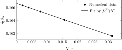
Figure 1: Numerical simulations for d=1𝑑1d=1; the fit was performed using the three parameters fit function f1(2)(N)=α1(2)+e1(2)N+cN2subscriptsuperscript𝑓21𝑁subscriptsuperscript𝛼21superscriptsubscript𝑒12𝑁𝑐superscript𝑁2f^{(2)}_{1}(N)=\alpha^{(2)}_{1}+\frac{e_{1}^{(2)}}{N}+\frac{c}{N^{2}}.

Let us consider the Ebmp in dimension d=1𝑑1d=1. In low dimensions, that is for d=1,2𝑑12d=1,2, the optimal cost is no longer a subadditive quantity and the fluctuations of the density of points are dominant Houdayer et al. (1998). Moreover, for d=1𝑑1d=1, the optimal cost is also not self-averaging Houdayer et al. (1998), while for d=2𝑑2d=2 this is still an open question.

In one dimension the structure of the optimal matching is known Houdayer et al. (1998); Boniolo2014: for any p>1𝑝1p>1 and using open boundary conditions, the optimal matching is the one associating the k𝑘k-th blue point to the k𝑘k-th red point, ordering the points from left to right along the line. This consideration leads to the prediction βN(2)(1)=O(Np2)subscriptsuperscript𝛽2𝑁1𝑂superscript𝑁𝑝2\beta^{(2)}_{N}(1)=O(N^{\frac{p}{2}}) for the leading behaviour with generic cost exponent p𝑝p. For closed periodic boundary conditions, the case we are considering, a similar scenario holds: enumerating the red points and the blue points clockwise or anticlockwise, the optimal matching is given by a cyclic permutation, with offset to be determined by the optimality condition.

The one-dimensional case constitutes the simplest application of our formula, Eq. (16), since this is the only where the sum is not divergent. We obtain straightforwardly

βN(2)(1)Nπ2n=1+1n2=N6.similar-tosubscriptsuperscript𝛽2𝑁1𝑁superscript𝜋2superscriptsubscript𝑛11superscript𝑛2𝑁6\beta^{(2)}_{N}(1)\sim\frac{N}{\pi^{2}}\sum_{n=1}^{+\infty}\frac{1}{n^{2}}=\frac{N}{6}. (17)

This is indeed the exact asymptotic behaviour of βNsubscript𝛽𝑁\beta_{N} Boniolo2014, and it is a first validation of our very simple ansatz, Eq. (15): we were able to catch both the anomalous scaling O(N)𝑂𝑁O\left(N\right) and its correct prefactor.

We checked the validity of Eq. (17) averaging the optimal cost of the Ebmp given by an exact algorithm Dezső et al. (2011) for system sizes up to N=2048𝑁2048N=2048: here and in the following numerical simulations were performed using a C++ code and the open source Lemon Graph Library Dezső et al. (2011). We found the numerical data for 1NβN1𝑁subscript𝛽𝑁\frac{1}{N}\beta_{N} to be well approximated by a three parameters fitting function of the form f1(2)(N)=α1(2)+e1(2)N+cN2subscriptsuperscript𝑓21𝑁subscriptsuperscript𝛼21subscriptsuperscript𝑒21𝑁𝑐superscript𝑁2f^{(2)}_{1}(N)=\alpha^{(2)}_{1}+\frac{e^{(2)}_{1}}{N}+\frac{c}{N^{2}}, where an additional correction of higher order is included. From a least square fit we obtained the coefficient α1(2)=0.166668(3)subscriptsuperscript𝛼210.1666683\alpha^{(2)}_{1}=0.166668(3), in perfect agreement with our analytical prediction (see Figure 1).

Once we verified the validity of Eq. (17), we used it to extrapolate the subleading coefficient e1(2)subscriptsuperscript𝑒21e^{(2)}_{1}, fixing α1(2)=16subscriptsuperscript𝛼2116\alpha^{(2)}_{1}=\frac{1}{6} and using the fitting function f1(2)(N)subscriptsuperscript𝑓21𝑁f^{(2)}_{1}(N) with two free parameters (see Figure 1 and Table 1).

II.2.2 Case d=2𝑑2d=2

Refer to caption
(a)  Numerical data for βN(2)(2)subscriptsuperscript𝛽2𝑁2\beta^{(2)}_{N}(2).
Refer to caption
(b)  Numerical results for βN(2)(2)lnN2πsubscriptsuperscript𝛽2𝑁2𝑁2𝜋\beta^{(2)}_{N}(2)-\frac{\ln N}{2\pi}.
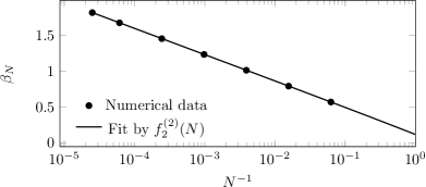
Figure 2: Numerical simulations for d=2𝑑2d=2. We fitted our numerical data for βN(2)(2)subscriptsuperscript𝛽2𝑁2\beta^{(2)}_{N}(2) using the function f2(2)(N)=alnN+e2(2)+blnNsubscriptsuperscript𝑓22𝑁𝑎𝑁superscriptsubscript𝑒22𝑏𝑁f^{(2)}_{2}(N)=a\ln N+e_{2}^{(2)}+\frac{b}{\ln{N}}. The 1lnN1𝑁\frac{1}{\ln{N}} correction was suggested by the right hand plot.

As already stated in the Introduction, in dimension 222 we have that βN=O(lnN)subscript𝛽𝑁𝑂𝑁\beta_{N}=O\left(\ln N\right). In this paragraph we will show how to derive this scaling from our ansatz, Eq. (16), and we will also obtain the corresponding prefactor. The sum appearing in Eq. (16) diverges in dimension 222 and above, therefore we have to find a suitable regularization to give meaning to the expression. The regularization procedure presents some peculiarities at d=2𝑑2d=2 from which the anomalous scaling arises.

We choose a regularizing smooth function F(x)𝐹𝑥F(x) such that F(0)=1𝐹01F(0)=1 and F(x)0𝐹𝑥0F(x)\to 0 for x+𝑥x\to+\infty. The function has to decrease rapidly enough to make the series 𝐧2{𝟎}1𝐧2F(2π𝐧2π1)subscript𝐧superscript201superscriptnorm𝐧2𝐹2𝜋norm𝐧2𝜋superscript1\sum_{\mathbf{n}\in\mathbb{Z}^{2}\setminus\{\mathbf{0}\}}\frac{1}{{\left\|\mathbf{n}\right\|}^{2}}F\left(2\pi{\left\|\mathbf{n}\right\|}\over 2\pi\ell^{-1}\right) converge: here we introduced a cut-off in momentum space, 2π12𝜋superscript12\pi\ell^{-1}, where 1N1𝑁\ell\equiv{1\over\sqrt{N}} is the characteristic length for the system, being \ell of the order of the average distance between a blue point and the nearest red point. Clearly 2π1+2𝜋superscript12\pi\ell^{-1}\to+\infty for N+𝑁N\to+\infty. Finally, let us denote by 𝒩d(r)=|{𝐱d{𝟎}|𝐱<r}|subscript𝒩𝑑𝑟conditional-set𝐱superscript𝑑0norm𝐱𝑟\mathcal{N}_{d}(r)={\left|\{\mathbf{x}\in\mathbb{Z}^{d}\setminus\{\mathbf{0}\}|{\left\|\mathbf{x}\right\|}<r\}\right|}, the number of lattice points (excluded the origin) included in a ball of radius r𝑟r centred in the origin in dimension d𝑑d. Then, for arbitrary a(0,1)𝑎01a\in(0,1), we can write

𝐧2{𝟎}1𝐧2F(𝐧N)subscript𝐧superscript201superscriptnorm𝐧2𝐹norm𝐧𝑁\displaystyle\sum_{\mathbf{n}\in\mathbb{Z}^{2}\setminus\{\mathbf{0}\}}\frac{1}{{\left\|\mathbf{n}\right\|}^{2}}F\left(\frac{{\left\|\mathbf{n}\right\|}}{\sqrt{N}}\right) =limRaR1r2F(rN)[𝒩2(r)r2πr]dr+2πaF(rN)drrabsentsubscript𝑅superscriptsubscript𝑎𝑅1superscript𝑟2𝐹𝑟𝑁delimited-[]subscript𝒩2𝑟𝑟2𝜋𝑟d𝑟2𝜋superscriptsubscript𝑎𝐹𝑟𝑁d𝑟𝑟\displaystyle=\lim_{R\to\infty}\int_{a}^{R}\frac{1}{r^{2}}\,F\left(\frac{r}{\sqrt{N}}\right)\left[\frac{\partial\mathcal{N}_{2}(r)}{\partial r}-2\pi r\right]\operatorname{d}r+2\pi\int_{a}^{\infty}F\left(\frac{r}{\sqrt{N}}\right)\frac{\operatorname{d}r}{r} (18)
limRaR1r2[𝒩2(r)r2πr]dr+2πaNF(r)rdr,absentsubscript𝑅superscriptsubscript𝑎𝑅1superscript𝑟2delimited-[]subscript𝒩2𝑟𝑟2𝜋𝑟d𝑟2𝜋superscriptsubscript𝑎𝑁𝐹𝑟𝑟d𝑟\displaystyle\approx\lim_{R\to\infty}\int_{a}^{R}\frac{1}{r^{2}}\left[\frac{\partial\mathcal{N}_{2}(r)}{\partial r}-2\pi r\right]\operatorname{d}r+2\pi\int_{\frac{a}{\sqrt{N}}}^{\infty}\frac{F(r)}{r}\operatorname{d}r,

where we have isolated in the last term the singular part of the series. The first integral in the right hand side is well behaved: indeed, aR1r2[𝒩2(r)r2πr]dr=𝒩2(r)πr2r2|aR+2aR𝒩2(r)πr2r3superscriptsubscript𝑎𝑅1superscript𝑟2delimited-[]subscript𝒩2𝑟𝑟2𝜋𝑟d𝑟evaluated-atsubscript𝒩2𝑟𝜋superscript𝑟2superscript𝑟2𝑎𝑅2superscriptsubscript𝑎𝑅subscript𝒩2𝑟𝜋superscript𝑟2superscript𝑟3\int_{a}^{R}\frac{1}{r^{2}}\left[\frac{\partial\mathcal{N}_{2}(r)}{\partial r}-2\pi r\right]\operatorname{d}r=\left.\frac{\mathcal{N}_{2}(r)-\pi r^{2}}{r^{2}}\right|_{a}^{R}+2\int_{a}^{R}\frac{\mathcal{N}_{2}(r)-\pi r^{2}}{r^{3}}. Both the first and the second term are finite in the R𝑅R\to\infty limit due to the fact that Hardy (1999) 𝒩2(r)πr21+22πrsubscript𝒩2𝑟𝜋superscript𝑟2122𝜋𝑟\mathcal{N}_{2}(r)-\pi r^{2}\leq 1+2\sqrt{2}\pi r. Therefore we have

𝐧2{𝟎}1𝐧2F(𝐧N)a+2r3[𝒩2(r)πr2]dr+πlogNa2e+2π1F(r)rdr.subscript𝐧superscript201superscriptnorm𝐧2𝐹norm𝐧𝑁superscriptsubscript𝑎2superscript𝑟3delimited-[]subscript𝒩2𝑟𝜋superscript𝑟2d𝑟𝜋𝑁superscript𝑎2e2𝜋superscriptsubscript1𝐹𝑟𝑟d𝑟\sum_{\mathbf{n}\in\mathbb{Z}^{2}\setminus\{\mathbf{0}\}}\frac{1}{{\left\|\mathbf{n}\right\|}^{2}}F\left(\frac{{\left\|\mathbf{n}\right\|}}{\sqrt{N}}\right)\approx\int_{a}^{+\infty}\frac{2}{r^{3}}\,\left[\mathcal{N}_{2}(r)-\pi r^{2}\right]\operatorname{d}r+\pi\log\frac{N}{a^{2}\operatorname{e}}+2\pi\int_{1}^{\infty}\frac{F(r)}{r}\operatorname{d}r. (19)

Eq. (16) for the case d=2𝑑2d=2 can then be rewritten as

βN(2)(2)lnN2π+e2(2).similar-tosubscriptsuperscript𝛽2𝑁2𝑁2𝜋superscriptsubscript𝑒22\beta^{(2)}_{N}(2)\sim\frac{\ln N}{2\pi}+e_{2}^{(2)}. (20)

where e2(2)superscriptsubscript𝑒22e_{2}^{(2)} is some constant. To our knowledge the result limNβN(2)(2)lnN=12πsubscript𝑁subscriptsuperscript𝛽2𝑁2𝑁12𝜋\lim_{N\to\infty}\frac{\beta^{(2)}_{N}(2)}{\ln N}=\frac{1}{2\pi} is new to the literature.

The validity of Eq. (20) has been confirmed by numerical simulation with system sizes up to N=4104𝑁4superscript104N=4\cdot 10^{4}. We found a three parameter function of the form f2(2)(N)=alnN+e2(2)+blnNsubscriptsuperscript𝑓22𝑁𝑎𝑁subscriptsuperscript𝑒22𝑏𝑁f^{(2)}_{2}(N)=a\ln N+e^{(2)}_{2}+\frac{b}{\ln{N}} to be the best suited to fit the data for βNsubscript𝛽𝑁\beta_{N}. From a least square fit we obtain the coefficient 2πa=1.0004(6)2𝜋𝑎1.000462\pi a=1.0004(6), in perfect agreement with our analytical prediction (see Figure 2). Once verified the validity of Eq. (20), we used it to extrapolate the subleading coefficient e2(2)subscriptsuperscript𝑒22e^{(2)}_{2}, fixing a=12π𝑎12𝜋a=\frac{1}{2\pi} and fitting the other two parameters (see Figure 1 and Table 1).

II.2.3 Case d>2𝑑2d>2

Refer to caption
(a)  d=3𝑑3d=3.
Refer to caption
(b)  d=4𝑑4d=4.
Refer to caption
(c)  d=5𝑑5d=5.
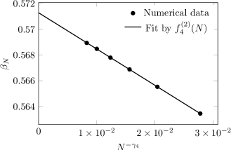
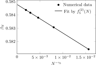
Figure 3: Numerical simulations for d>2𝑑2d>2. We fitted our numerical data for βN(2)(d)subscriptsuperscript𝛽2𝑁𝑑\beta^{(2)}_{N}(d) using the function fd(2)(N)=ed(2)+αd(2)Nγd+cNsubscriptsuperscript𝑓2𝑑𝑁subscriptsuperscript𝑒2𝑑subscriptsuperscript𝛼2𝑑superscript𝑁subscript𝛾𝑑𝑐𝑁f^{(2)}_{d}(N)=e^{(2)}_{d}+\alpha^{(2)}_{d}N^{-\gamma_{d}}+\frac{c}{N}. The expected value for αd(2)subscriptsuperscript𝛼2𝑑\alpha^{(2)}_{d} was 12π2ζd(1)12superscript𝜋2subscript𝜁𝑑1\frac{1}{2\pi^{2}}\zeta_{d}(1).
d=1𝑑1d=1 d=2𝑑2d=2 d=3𝑑3d=3 d=4𝑑4d=4 d=5𝑑5d=5
12π2ζd(1)12superscript𝜋2subscript𝜁𝑑1\frac{1}{2\pi^{2}}\zeta_{d}(1) 1616\frac{1}{6} - 0.451570.45157-0.45157\dots 0.280910.28091-0.28091\dots 0.214230.21423-0.21423\dots
αd(2)subscriptsuperscript𝛼2𝑑\alpha^{(2)}_{d} 0.166668(3)0.16666830.166668(3) - 0.4489(16)0.448916-0.4489(16) 0.282(4)0.2824-0.282(4) 0.2139(13)0.213913-0.2139(13)
ed(2)subscriptsuperscript𝑒2𝑑e^{(2)}_{d} 0.1645(13)0.164513-0.1645(13) 0.1332(5)0.133250.1332(5) 0.66251(2)0.6625120.66251(2) 0.571284(6)0.57128460.571284(6) 0.584786(2)0.58478620.584786(2)
Table 1: Results of numerical simulations for p=2𝑝2p=2. In the first line the analytical prediction for αd(2)subscriptsuperscript𝛼2𝑑\alpha^{(2)}_{d} for d2𝑑2d\neq 2 is presented.

In dimensions greater than 222 the average optimal cost has the leading scaling EN(2)(d)=O(N2d)superscriptsubscript𝐸𝑁2𝑑𝑂superscript𝑁2𝑑E_{N}^{(2)}(d)=O(N^{-\frac{2}{d}}) that one could expect from very simple arguments Mézard and Parisi (1985), as already stated in the introduction. This is in fact the scaling obtained if each point is matched to one of its nearest points of different type, being their distance of order O(N1d)𝑂superscript𝑁1𝑑O(N^{-\frac{1}{d}}). Moreover it has been proven, using standard sub-additivity arguments, that βNsubscript𝛽𝑁\beta_{N} is a self-averaging quantity and has a finite limit for d>2𝑑2d>2 Houdayer et al. (1998). We will show that our ansatz Eq. (15) accounts for the subleading corrections to βNsubscript𝛽𝑁\beta_{N}.

For d2𝑑2d\geq 2 the series 𝐧d{𝟎}1𝐧2subscript𝐧superscript𝑑01superscriptnorm𝐧2\sum_{\mathbf{n}\in\mathbb{Z}^{d}\setminus\{\mathbf{0}\}}\frac{1}{{\left\|\mathbf{n}\right\|}^{2}} is divergent. As in the previous paragraph, we use a sufficiently rapidly decaying function F(x)𝐹𝑥F(x), with limxF(x)=0subscript𝑥𝐹𝑥0\lim_{x\to\infty}F(x)=0 and limx0F(x)=1subscript𝑥0𝐹𝑥1\lim_{x\to 0}F(x)=1, to regularize it. The characteristic length of the system is given by =1Nd1𝑑𝑁\ell=\frac{1}{\sqrt[d]{N}}. Denoting, as before, by 𝒩d(r)subscript𝒩𝑑𝑟\mathcal{N}_{d}(r) the number of lattice points inside a sphere centred in the origin and of radius r𝑟r, with the exclusion of the origin itself, we can write the following:

𝐧d{𝟎}1𝐧2F(𝐧Nd)subscript𝐧superscript𝑑01superscriptnorm𝐧2𝐹norm𝐧𝑑𝑁\displaystyle\sum_{\mathbf{n}\in\mathbb{Z}^{d}\setminus\{\mathbf{0}\}}\frac{1}{{\left\|\mathbf{n}\right\|}^{2}}F\left(\frac{{\left\|\mathbf{n}\right\|}}{\sqrt[d]{N}}\right) =0+1r2F(rNd)[𝒩d(r)rSdrd1]dr+Nd2dSd0F(r)rd3drabsentsuperscriptsubscript01superscript𝑟2𝐹𝑟𝑑𝑁delimited-[]subscript𝒩𝑑𝑟𝑟subscript𝑆𝑑superscript𝑟𝑑1d𝑟superscript𝑁𝑑2𝑑subscript𝑆𝑑superscriptsubscript0𝐹𝑟superscript𝑟𝑑3d𝑟\displaystyle=\int_{0}^{+\infty}\frac{1}{r^{2}}\,F\left(\frac{r}{\sqrt[d]{N}}\right)\left[\frac{\partial\mathcal{N}_{d}(r)}{\partial r}-S_{d}\,r^{d-1}\right]\operatorname{d}r+N^{d-2\over d}S_{d}\int_{0}^{\infty}F\left(r\right)r^{d-3}\operatorname{d}r (21)
0+1r2[𝒩d(r)rSdrd1]dr+Nd2dSd0F(r)rd3dr,absentsuperscriptsubscript01superscript𝑟2delimited-[]subscript𝒩𝑑𝑟𝑟subscript𝑆𝑑superscript𝑟𝑑1d𝑟superscript𝑁𝑑2𝑑subscript𝑆𝑑superscriptsubscript0𝐹𝑟superscript𝑟𝑑3d𝑟\displaystyle\approx\int_{0}^{+\infty}\frac{1}{r^{2}}\left[\frac{\partial\mathcal{N}_{d}(r)}{\partial r}-S_{d}\,r^{d-1}\right]\operatorname{d}r+N^{d-2\over d}S_{d}\int_{0}^{\infty}F\left(r\right)r^{d-3}\operatorname{d}r,

where Sd=2πd2Γ(d2)subscript𝑆𝑑2superscript𝜋𝑑2Γ𝑑2S_{d}=\frac{2\pi^{\frac{d}{2}}}{\Gamma\left(\frac{d}{2}\right)} is the unit sphere surface in d𝑑d dimensions. The last term in Eq. (21) gives the leading-order contribution to βNsubscript𝛽𝑁\beta_{N}, but in our formalism it cannot be explicitly computed since it depends on the choice of the regularizing function F(x)𝐹𝑥F(x). We name the other integral on the right hand side as

Σd0+1r2[𝒩d(r)rSdrd1]dr.subscriptΣ𝑑superscriptsubscript01superscript𝑟2delimited-[]subscript𝒩𝑑𝑟𝑟subscript𝑆𝑑superscript𝑟𝑑1d𝑟\Sigma_{d}\equiv\int_{0}^{+\infty}\frac{1}{r^{2}}\left[\frac{\partial\mathcal{N}_{d}(r)}{\partial r}-S_{d}\,r^{d-1}\right]\operatorname{d}r. (22)

ΣdsubscriptΣ𝑑\Sigma_{d} gives the first subleading correction to the leading scaling of βNsubscript𝛽𝑁\beta_{N}. Moreover, it can be shown (see appendix A) that Σd=ζd(1)subscriptΣ𝑑subscript𝜁𝑑1\Sigma_{d}=\zeta_{d}(1), the analytic continuation to the point s=1𝑠1s=1 of the function

ζd(s)𝐧d{𝟎}1𝐧2sfor Res>d2.formulae-sequencesubscript𝜁𝑑𝑠subscript𝐧superscript𝑑01superscriptnorm𝐧2𝑠for Re𝑠𝑑2\zeta_{d}(s)\equiv\sum_{\mathbf{n}\in\mathbb{Z}^{d}\setminus\{\mathbf{0}\}}\frac{1}{{\left\|\mathbf{n}\right\|}^{2s}}\qquad\text{for }\operatorname{Re}s>\frac{d}{2}. (23)

The previous function is a particular case of a more general class of ζ𝜁\zeta functions, called Epstein zeta functions. Therefore we are able to compute analytically the subleading behaviour of βNsubscript𝛽𝑁\beta_{N} for d>2𝑑2d>2,

βN(2)(d)ed(2)+ζd(1)2π2Nγd,γdd2d.formulae-sequencesimilar-tosubscriptsuperscript𝛽2𝑁𝑑superscriptsubscript𝑒𝑑2subscript𝜁𝑑12superscript𝜋2superscript𝑁subscript𝛾𝑑subscript𝛾𝑑𝑑2𝑑\beta^{(2)}_{N}(d)\sim e_{d}^{(2)}+\frac{\zeta_{d}(1)}{2\pi^{2}N^{\gamma_{d}}},\qquad\gamma_{d}\equiv\frac{d-2}{d}. (24)

The expression for ζd(1)subscript𝜁𝑑1\zeta_{d}(1) is given by Eq. (33), while the intensive costs ed(2)superscriptsubscript𝑒𝑑2e_{d}^{(2)} have to be determined numerically. Note that for d+𝑑d\to+\infty we recover the correct meanfield scaling behaviour already analyzed by Houdayer et al. (1998) for the random assignment problem, i.e. γd1subscript𝛾𝑑1\gamma_{d}\to 1. However, for finite d𝑑d, the scaling behaviour can be very different from the mean field one.

We verified the validity of Eq. (24) with numerical simulation on systems with sizes up to N=10648𝑁10648N=10648 in dimension d=3𝑑3d=3, N=14641𝑁14641N=14641 in dimension d=4𝑑4d=4 and N=32768𝑁32768N=32768 in dimension d=5𝑑5d=5. We used three parameter functions of the form fd(2)(N)=ed(2)+αd(2)Nγd+cNsubscriptsuperscript𝑓2𝑑𝑁subscriptsuperscript𝑒2𝑑subscriptsuperscript𝛼2𝑑superscript𝑁subscript𝛾𝑑𝑐𝑁f^{(2)}_{d}(N)=e^{(2)}_{d}+\frac{\alpha^{(2)}_{d}}{N^{\gamma_{d}}}+\frac{c}{N} to fit our data for βN(2)(d)subscriptsuperscript𝛽2𝑁𝑑\beta^{(2)}_{N}(d). The scaling exponents γdsubscript𝛾𝑑\gamma_{d} are readily confirmed to be the right ones (see Figure 3) and the fitted coefficients αd(2)subscriptsuperscript𝛼2𝑑\alpha^{(2)}_{d} are in strong agreement with the analytical prediction ζd(1)2π2subscript𝜁𝑑12superscript𝜋2\frac{\zeta_{d}(1)}{2\pi^{2}} (Table 1). Then we fixed the αd(2)=ζd(1)2π2subscriptsuperscript𝛼2𝑑subscript𝜁𝑑12superscript𝜋2\alpha^{(2)}_{d}=\frac{\zeta_{d}(1)}{2\pi^{2}} in fd(2)(N)subscriptsuperscript𝑓2𝑑𝑁f^{(2)}_{d}(N) to extrapolate the extensive coefficients ed(2)subscriptsuperscript𝑒2𝑑e^{(2)}_{d}, reported in Table 1.

III Results for generic p𝑝p

Refer to caption
(a)  d=3𝑑3d=3.
Refer to caption
(b)  d=4𝑑4d=4.
Refer to caption
(c)  d=5𝑑5d=5.
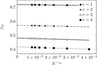
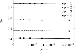
Figure 4: Numerical simulations for d>2𝑑2d>2. We fitted our numerical data for βN(p)(d)subscriptsuperscript𝛽𝑝𝑁𝑑\beta^{(p)}_{N}(d) using the function fd(p)(N)=ed(p)+αd(p)Nγd+cNsuperscriptsubscript𝑓𝑑𝑝𝑁superscriptsubscript𝑒𝑑𝑝superscriptsubscript𝛼𝑑𝑝superscript𝑁subscript𝛾𝑑𝑐𝑁f_{d}^{(p)}(N)=e_{d}^{(p)}+\alpha_{d}^{(p)}N^{-\gamma_{d}}+\frac{c}{N}. We plotted the results obtained for p=1,3,4𝑝134p=1,3,4. Fit results are presented in Table 2.
p=1𝑝1p=1 p=3𝑝3p=3 p=4𝑝4p=4
d=3𝑑3d=3 d=4𝑑4d=4 d=5𝑑5d=5 d=3𝑑3d=3 d=4𝑑4d=4 d=5𝑑5d=5 d=3𝑑3d=3 d=4𝑑4d=4 d=5𝑑5d=5
αd(p)subscriptsuperscript𝛼𝑝𝑑\alpha^{(p)}_{d} 0.233(2)0.2332-0.233(2) 0.152(17)0.15217-0.152(17) 0.127(16)0.12716-0.127(16) 0.652(3)0.6523-0.652(3) 0.36(1)0.361-0.36(1) 0.28(4)0.284-0.28(4) 0.863(3)0.8633-0.863(3) 0.44(2)0.442-0.44(2) 0.34(1)0.341-0.34(1)
ed(p)subscriptsuperscript𝑒𝑝𝑑e^{(p)}_{d} 0.7472(2)0.747220.7472(2) 0.7181(2)0.718120.7181(2) 0.73905(5)0.7390550.73905(5) 0.6313(2)0.631320.6313(2) 0.4804(1)0.480410.4804(1) 0.4830(1)0.483010.4830(1) 0.6286(2)0.628620.6286(2) 0.4183(2)0.418320.4183(2) 0.41043(4)0.4104340.41043(4)
Table 2: Results of the fit of numerical data for βN(p)(d)subscriptsuperscript𝛽𝑝𝑁𝑑\beta^{(p)}_{N}(d) by a function of the form fd(p)(N)=ed(p)+αd(p)Nγd+cNsubscriptsuperscript𝑓𝑝𝑑𝑁superscriptsubscript𝑒𝑑𝑝superscriptsubscript𝛼𝑑𝑝superscript𝑁subscript𝛾𝑑𝑐𝑁f^{(p)}_{d}(N)=e_{d}^{(p)}+\frac{\alpha_{d}^{(p)}}{N^{\gamma_{d}}}+\frac{c}{N}.

The asymptotic form we proposed for the average optimal cost EN(2)(d)superscriptsubscript𝐸𝑁2𝑑E_{N}^{(2)}(d) in the Ebmp with quadratic costs and periodic boundary conditions, Eq. (15), could not be extended to cover the case of generic cost exponent p𝑝p. Nonetheless, our numerical simulations give strong evidence that, for d>2𝑑2d>2 and any p>0𝑝0p>0, βNsubscript𝛽𝑁\beta_{N} has the asymptotic form

βN(p)(d)ed(p)+αd(p)Nγd,γdd2d.formulae-sequencesimilar-tosubscriptsuperscript𝛽𝑝𝑁𝑑superscriptsubscript𝑒𝑑𝑝superscriptsubscript𝛼𝑑𝑝superscript𝑁subscript𝛾𝑑subscript𝛾𝑑𝑑2𝑑\beta^{(p)}_{N}(d)\sim e_{d}^{(p)}+\frac{\alpha_{d}^{(p)}}{N^{\gamma_{d}}},\qquad\gamma_{d}\equiv\frac{d-2}{d}. (25)

We thus find the same scaling exponent γdsubscript𝛾𝑑\gamma_{d} analytically predicted only for the case p=2𝑝2p=2. The nontrivial scaling exponent γdsubscript𝛾𝑑\gamma_{d} differs from the mean-field exponent γ=1subscript𝛾1\gamma_{\infty}=1 of the random link matching problem Parisi and Ratiéville (2002) and of the Eucliden monopartite matching Houdayer et al. (1998). The identification of the correct exponent γdsubscript𝛾𝑑\gamma_{d} is crucial to the extrapolation of ed(p)superscriptsubscript𝑒𝑑𝑝e_{d}^{(p)} from numerical data. Since in the literature a mean-field-like scaling has been considered Houdayer et al. (1998), we report in Table 2 the values of ed(p)superscriptsubscript𝑒𝑑𝑝e_{d}^{(p)} and αd(p)superscriptsubscript𝛼𝑑𝑝\alpha_{d}^{(p)} for different values of p𝑝p. They were obtained fitting βNsubscript𝛽𝑁\beta_{N} with functions of the form fd(p)(N)=ed(p)+αd(p)Nγd+cNsubscriptsuperscript𝑓𝑝𝑑𝑁superscriptsubscript𝑒𝑑𝑝superscriptsubscript𝛼𝑑𝑝superscript𝑁subscript𝛾𝑑𝑐𝑁f^{(p)}_{d}(N)=e_{d}^{(p)}+\frac{\alpha_{d}^{(p)}}{N^{\gamma_{d}}}+\frac{c}{N}. In Figure 4 we plot βN(1)superscriptsubscript𝛽𝑁1\beta_{N}^{(1)}, βN(3)superscriptsubscript𝛽𝑁3\beta_{N}^{(3)} and βN(4)superscriptsubscript𝛽𝑁4\beta_{N}^{(4)} for d=3,4,5𝑑345d=3,4,5, along with the data already presented for p=2𝑝2p=2 for comparison. The scaling exponent γd=d2dsubscript𝛾𝑑𝑑2𝑑\gamma_{d}=\frac{d-2}{d} is confirmed by our simulations. Generalizing the case p=2𝑝2p=2, we therefore conjecture that the optimal cost as a function of the difference of the density of point δρ(𝐱)𝛿𝜌𝐱\delta\rho(\mathbf{x}), for |δρ(𝐱)|1much-less-than𝛿𝜌𝐱1{\left|\delta\rho(\mathbf{x})\right|}\ll 1 and in dimension d>2𝑑2d>2, can be approximated by

N(p)[δρ^]Ad(p)𝐧d{𝟎}|δρ^𝐧|24π2𝐧2.subscriptsuperscript𝑝𝑁delimited-[]𝛿^𝜌subscriptsuperscript𝐴𝑝𝑑subscript𝐧superscript𝑑0superscript𝛿subscript^𝜌𝐧24superscript𝜋2superscriptnorm𝐧2\mathcal{E}^{(p)}_{N}[\delta\hat{\rho}]\equiv A^{(p)}_{d}\sum_{\mathbf{n}\in\mathbb{Z}^{d}\setminus\{\mathbf{0}\}}\frac{{\left|\delta\hat{\rho}_{\mathbf{n}}\right|}^{2}}{4\pi^{2}{\left\|\mathbf{n}\right\|}^{2}}. (26)

where Ad(p)subscriptsuperscript𝐴𝑝𝑑A^{(p)}_{d} are unknown parameters. From last equation, the asymptotic form Eq. (25) for βNsubscript𝛽𝑁\beta_{N} can be derived, but at odds with the case p=2𝑝2p=2 where Ad(2)1subscriptsuperscript𝐴2𝑑1A^{(2)}_{d}\equiv 1 for any d𝑑d, the lack of knowledge of the value of the parameters Ad(p)subscriptsuperscript𝐴𝑝𝑑A^{(p)}_{d} forbids the analytic prediction of the subleading coefficients αd(p)superscriptsubscript𝛼𝑑𝑝\alpha_{d}^{(p)}. We also notice that Eq. (26) cannot be extended to dimensions d=1,2𝑑12d=1,2, since it is incompatible with the scaling scenario depicted in Eq. (4).

The ansatz given in Eq. (15) for p=2𝑝2p=2 has been a posteriori confirmed by the correct prediction of both the exponents γdsubscript𝛾𝑑\gamma_{d} and the subleading coefficients αd(2)superscriptsubscript𝛼𝑑2\alpha_{d}^{(2)}. On the other hand, for generic p𝑝p, the ansatz (26) is only supported by the fact that it gives the correct exponents γdsubscript𝛾𝑑\gamma_{d}, which is the reason itself why it was introduced. Therefore we tried to verify the internal consistence of Eq. (26). In fact after some algebraic manipulations and averaging over the disorder one can derive

Ad(p)𝐧2πN22(EN(p)[π;{𝐫i,𝐛i}]EN(p))|δρ^𝐧|2¯.similar-tosubscriptsuperscript𝐴𝑝𝑑superscriptnorm𝐧2𝜋superscript𝑁22¯subscriptsuperscript𝐸𝑝𝑁superscript𝜋subscript𝐫𝑖subscript𝐛𝑖superscriptsubscript𝐸𝑁𝑝superscript𝛿subscript^𝜌𝐧2A^{(p)}_{d}\sim\frac{{\left\|\mathbf{n}\right\|}^{2}\pi N^{2}}{2}\ \overline{\left(E^{(p)}_{N}[\pi^{*};\{\mathbf{r}_{i},\mathbf{b}_{i}\}]-E_{N}^{(p)}\right){\left|\delta\hat{\rho}_{\mathbf{n}}\right|}^{2}}. (27)

where we used the notation introduced in Eq. (3). We computed numerically the right-hand side of the previous equation for d=3𝑑3d=3 and sizes up to N=10648𝑁10648N=10648. The computation is numerically quite heavy since the density fluctuation are small. While the left-hand side of Eq. (27) is independent of the mode 𝐧𝐧\mathbf{n} in the large N𝑁N limit, we observed a finite size effect that seemed to be best accounted for by the scaling form A3(p)(𝐧,N)A3(p)+b1N3+c(𝐧N3)2similar-tosubscriptsuperscript𝐴𝑝3𝐧𝑁subscriptsuperscript𝐴𝑝3𝑏13𝑁𝑐superscriptnorm𝐧3𝑁2A^{(p)}_{3}(\mathbf{n},N)\sim A^{(p)}_{3}+b\frac{1}{\sqrt[3]{N}}+c\left(\frac{{\left\|\mathbf{n}\right\|}}{\sqrt[3]{N}}\right)^{2}. Using this three parameters function to fit our whole set of data (𝐧<10norm𝐧10{\left\|\mathbf{n}\right\|}<10) at fixed p𝑝p, we extrapolate the values of A3(p)subscriptsuperscript𝐴𝑝3A^{(p)}_{3} that we report in Table 3. In the same table we compare these extrapolations with the predictions steaming from Eq. (26), that is Ad(p)=αd(p)αd(2)=αd(p)2πζd(1)subscriptsuperscript𝐴𝑝𝑑subscriptsuperscript𝛼𝑝𝑑subscriptsuperscript𝛼2𝑑subscriptsuperscript𝛼𝑝𝑑2𝜋subscript𝜁𝑑1A^{(p)}_{d}=\frac{\alpha^{(p)}_{d}}{\alpha^{(2)}_{d}}=\alpha^{(p)}_{d}\frac{2\pi}{\zeta_{d}(1)}, where the coefficients αd(p)subscriptsuperscript𝛼𝑝𝑑\alpha^{(p)}_{d} where computed in Table 2. The agreement between the two different sets of values is quantitatively and qualitatively good, even though we cannot definitively affirm the validity of Eq. (26) due to the complexity and imprecision of the procedure utilized to test it. A more sound verification would be to manually excite one of the modes through the addition a position dependent shift of the form ϵ𝐧cos(2π𝐧𝐱)italic-ϵ𝐧2𝜋𝐧𝐱\epsilon\,\mathbf{n}\cos(2\pi\mathbf{n}\cdot\mathbf{x}) to each randomly generated point in one of the sets. One should then observe a linear response of the totat cost to the variation of ϵitalic-ϵ\epsilon as predicted by Eq. (26).

p=1𝑝1p=1 p=2𝑝2p=2 p=3𝑝3p=3 p=4𝑝4p=4
A3(p)subscriptsuperscript𝐴𝑝3A^{(p)}_{3} from Eq. (26) 0.516(5)0.51650.516(5) 111 1.44(1)1.4411.44(1) 1.908(4)1.90841.908(4)
A3(p)subscriptsuperscript𝐴𝑝3A^{(p)}_{3} from Eq. (27) 0.51(3)0.5130.51(3) 0.99(2)0.9920.99(2) 1.46(3)1.4631.46(3) 1.96(2)1.9621.96(2)
Table 3: Values of Ad(p)subscriptsuperscript𝐴𝑝𝑑A^{(p)}_{d} for d=3𝑑3d=3, extrapolated from Eqs. (26) and (27) respectively, as explained in the main text. The error in the second row are upscaled by a factor ten from those given by our fitting program (gnuplot), to assure the compatibility with the case p=2𝑝2p=2.

IV Conclusions and perspectives

In the present work we proposed a simple form for the asymptotic behaviour of the average optimal cost, EN(2)(d)subscriptsuperscript𝐸2𝑁𝑑E^{(2)}_{N}(d), in the Euclidean bipartite matching problem with quadratic costs and periodic boundary conditions. This ansatz, Eq. (15), contains no free parameters and leads to a strong set of predictions in every dimension, resumed in Eq. (6). The rescaled cost βN(2)(d)EN(2)N2dsubscriptsuperscript𝛽2𝑁𝑑subscriptsuperscript𝐸2𝑁superscript𝑁2𝑑\beta^{(2)}_{N}(d)\equiv\frac{E^{(2)}_{N}}{N^{-\frac{2}{d}}} for low dimensions is a diverging quantity in the Ebmp, at odds with the monopartite case. We were able to prove that limNβN(2)(1)N=16subscript𝑁subscriptsuperscript𝛽2𝑁1𝑁16\lim_{N\to\infty}\frac{\beta^{(2)}_{N}(1)}{N}=\frac{1}{6} and limNβN(2)(2)logN=12πsubscript𝑁subscriptsuperscript𝛽2𝑁2𝑁12𝜋\lim_{N\to\infty}\frac{\beta^{(2)}_{N}(2)}{\log N}=\frac{1}{2\pi} for d=1𝑑1d=1 and d=2𝑑2d=2 respectively. Above the critical dimension of the system, d=2𝑑2d=2, the rescaled cost βN(2)(d)subscriptsuperscript𝛽2𝑁𝑑\beta^{(2)}_{N}(d) has a finite limit which is inaccessible to our formalism. We were able though to determine analytically both the subleading scaling, O(Nγd)𝑂superscript𝑁subscript𝛾𝑑O(N^{-\gamma_{d}}) with γd=d2dsubscript𝛾𝑑𝑑2𝑑\gamma_{d}=\frac{d-2}{d}, and its prefactor ζd(1)2π2subscript𝜁𝑑12superscript𝜋2\frac{\zeta_{d}(1)}{2\pi^{2}}. All the above claims are overwhelmingly supported by numerical simulations.

Finally, we provided numerical evidences that, in dimension d>2𝑑2d>2, the subleading scaling exponent γdsubscript𝛾𝑑\gamma_{d} we predicted for the case of quadratic costs is the same for arbitrary cost exponent p𝑝p. This led us to extend the ansatz proposed for quadratic costs, Eq. (15), to the general form Eq. (25) for d>2𝑑2d>2. We tested numerically the validity of Eq. (25), obtaining good but not definitive results, therefore we proposed another numerical procedure that could give a firmer validation to the theory.

Although our scaling ansatz proved itself to be very powerful, as discussed above, a deeper theoretical investigation is required to derive analytically the limit of β(p)(d)superscript𝛽𝑝𝑑\beta^{(p)}(d) at large N𝑁N, not computable in our framework. Moreover, a rigorous justification of our simple ansatz is desirable and could be inspired by the considerations we made in Section II.1 on the Monge–Kantorovič problem.

Acknowledgements

The research leading to these results has received funding from the European Research Council under the European Union’s Seventh Framework Programme (FP7/2007-2013) / ERC grant agreement No. 247328. S.C. and G.S. are grateful to Luigi Ambrosio for useful and stimulating discussions.

Appendix A Evaluation of ΣdsubscriptΣ𝑑\Sigma_{d}

In this appendix we will show that, in dimension d>2𝑑2d>2, the function

ζd(s)=𝐧d{𝟎}1𝐧2s,subscript𝜁𝑑𝑠subscript𝐧superscript𝑑01superscriptnorm𝐧2𝑠\zeta_{d}(s)=\sum_{\mathbf{n}\in\mathbb{Z}^{d}\setminus\{\mathbf{0}\}}\frac{1}{{\left\|\mathbf{n}\right\|}^{2s}}, (28)

a particular Epstein zeta function defined for Res>d2Re𝑠𝑑2\operatorname{Re}s>\frac{d}{2}, analytically continued to the point s=1𝑠1s=1, takes the value of ΣdsubscriptΣ𝑑\Sigma_{d} defined in Eq. (22), i.e. ζd(1)=Σdsubscript𝜁𝑑1subscriptΣ𝑑\zeta_{d}(1)=\Sigma_{d}. Then we will derive an easily computable representation of the analytic continuation of ζd(s)subscript𝜁𝑑𝑠\zeta_{d}(s) which was already presented in the literature(Ajtai et al., 1984; Contino and Gambassi, 2003).

Let us fix d>2𝑑2d>2 and a>0𝑎0a>0. Then, for Res>d2Re𝑠𝑑2\operatorname{Re}s>\frac{d}{2}, we can rewrite Eq. (28) as

ζd(s)subscript𝜁𝑑𝑠\displaystyle\zeta_{d}(s) =limR+[𝐧d{0}𝐧R1𝐧2sSdaRrd1r2sdr+SdaRrd1r2sdr]absentsubscript𝑅delimited-[]superscriptsubscript𝐧superscript𝑑0norm𝐧𝑅1superscriptnorm𝐧2𝑠subscript𝑆𝑑superscriptsubscript𝑎𝑅superscript𝑟𝑑1superscript𝑟2𝑠d𝑟subscript𝑆𝑑superscriptsubscript𝑎𝑅superscript𝑟𝑑1superscript𝑟2𝑠d𝑟\displaystyle=\lim_{R\to+\infty}\left[\sum_{\mathbf{n}\in\mathbb{Z}^{d}\setminus\{0\}}^{{\left\|\mathbf{n}\right\|}\leq R}\frac{1}{{\left\|\mathbf{n}\right\|}^{2s}}-S_{d}\int_{a}^{R}\frac{r^{d-1}}{r^{2s}}\operatorname{d}r+S_{d}\int_{a}^{R}\frac{r^{d-1}}{r^{2s}}\operatorname{d}r\right] (29)
=limR+[𝐧d{0}𝐧R1𝐧2sSdaRrd1r2sdr]+Sdad2s2sd.absentsubscript𝑅delimited-[]superscriptsubscript𝐧superscript𝑑0norm𝐧𝑅1superscriptnorm𝐧2𝑠subscript𝑆𝑑superscriptsubscript𝑎𝑅superscript𝑟𝑑1superscript𝑟2𝑠d𝑟subscript𝑆𝑑superscript𝑎𝑑2𝑠2𝑠𝑑\displaystyle=\lim_{R\to+\infty}\left[\sum_{\mathbf{n}\in\mathbb{Z}^{d}\setminus\{0\}}^{{\left\|\mathbf{n}\right\|}\leq R}\frac{1}{{\left\|\mathbf{n}\right\|}^{2s}}-S_{d}\int_{a}^{R}\frac{r^{d-1}}{r^{2s}}\operatorname{d}r\right]+S_{d}\frac{a^{d-2s}}{2s-d}.

Assuming that the limit in the last equation exists also for Res<d2Re𝑠𝑑2\operatorname{Re}s<\frac{d}{2}, we have isolated the singular term. The analytic continuation of ζd(s)subscript𝜁𝑑𝑠\zeta_{d}(s) then reads

ζd(s)=limR+[𝐧d{0}𝐧R1𝐧2sSd0Rrd1r2sdr]for Res<d2,formulae-sequencesubscript𝜁𝑑𝑠subscript𝑅delimited-[]superscriptsubscript𝐧superscript𝑑0norm𝐧𝑅1superscriptnorm𝐧2𝑠subscript𝑆𝑑superscriptsubscript0𝑅superscript𝑟𝑑1superscript𝑟2𝑠d𝑟for Re𝑠𝑑2\zeta_{d}(s)=\lim_{R\to+\infty}\left[\sum_{\mathbf{n}\in\mathbb{Z}^{d}\setminus\{0\}}^{{\left\|\mathbf{n}\right\|}\leq R}\frac{1}{{\left\|\mathbf{n}\right\|}^{2s}}-S_{d}\int_{0}^{R}\frac{r^{d-1}}{r^{2s}}\operatorname{d}r\right]\qquad\text{for }\operatorname{Re}s<\frac{d}{2}, (30)

where to limit a0𝑎0a\to 0 has been taken. Note that, comparing the previous equation with Eq. (22), ζd(1)Σdsubscript𝜁𝑑1subscriptΣ𝑑\zeta_{d}(1)\equiv\Sigma_{d}. On the other hand, for Res>d2Re𝑠𝑑2\operatorname{Re}s>\frac{d}{2}

ζd(s)subscript𝜁𝑑𝑠\displaystyle\zeta_{d}(s) =𝐧d{𝟎}1Γ(s)0+zs1e𝐧2zdzabsentsubscript𝐧superscript𝑑01Γ𝑠superscriptsubscript0superscript𝑧𝑠1superscriptesuperscriptnorm𝐧2𝑧d𝑧\displaystyle=\sum_{\mathbf{n}\in\mathbb{Z}^{d}\setminus\{\mathbf{0}\}}\frac{1}{\Gamma(s)}\int_{0}^{+\infty}z^{s-1}\operatorname{e}^{-{\left\|\mathbf{n}\right\|}^{2}z}\operatorname{d}z (31)
=πsΓ(s)0+zs1(Θd(z)1)dz,absentsuperscript𝜋𝑠Γ𝑠superscriptsubscript0superscript𝑧𝑠1superscriptΘ𝑑𝑧1d𝑧\displaystyle=\frac{\pi^{s}}{\Gamma(s)}\int_{0}^{+\infty}z^{s-1}\left(\Theta^{d}(z)-1\right)\operatorname{d}z,

where Θ(z)Θ𝑧\Theta(z) is defined by Θ(z)n=+eπn2zϑ(0;iz)Θ𝑧superscriptsubscript𝑛superscripte𝜋superscript𝑛2𝑧italic-ϑ0𝑖𝑧\Theta(z)\equiv\sum_{n=-\infty}^{+\infty}\operatorname{e}^{-\pi n^{2}z}\equiv\vartheta(0;iz), where ϑ(τ;z)italic-ϑ𝜏𝑧\vartheta(\tau;z) is the Jacobi θ𝜃\theta function. Noticing that for z1much-less-than𝑧1z\ll 1 asymptotically we have Θ(z)1zsimilar-toΘ𝑧1𝑧\Theta(z)\sim\frac{1}{\sqrt{z}}, while Θ(z)1+2ezsimilar-toΘ𝑧12superscripte𝑧\Theta(z)\sim 1+2\operatorname{e}^{-z} for z1much-greater-than𝑧1z\gg 1, we can isolate the singular parts of ζd(s)subscript𝜁𝑑𝑠\zeta_{d}(s) writing

ζd(s)=πsΓ(s)[22sd1s+1+zs1(Θd(z)1)dz+01zs1(Θd(z)1zd2)dz].subscript𝜁𝑑𝑠superscript𝜋𝑠Γ𝑠delimited-[]22𝑠𝑑1𝑠superscriptsubscript1superscript𝑧𝑠1superscriptΘ𝑑𝑧1d𝑧superscriptsubscript01superscript𝑧𝑠1superscriptΘ𝑑𝑧1superscript𝑧𝑑2d𝑧\zeta_{d}(s)=\frac{\pi^{s}}{\Gamma(s)}\left[\frac{2}{2s-d}-\frac{1}{s}+\int_{1}^{+\infty}z^{s-1}\left(\Theta^{d}(z)-1\right)\operatorname{d}z+\int_{0}^{1}z^{s-1}\left(\Theta^{d}(z)-\frac{1}{z^{\frac{d}{2}}}\right)\operatorname{d}z\right]. (32)

The last expression can be readily continued to the region Res<d2Re𝑠𝑑2\operatorname{Re}s<\frac{d}{2}. Using the property tΘ(t)=Θ(t1)𝑡Θ𝑡Θsuperscript𝑡1\sqrt{t}\,\Theta(t)=\Theta(t^{-1}), we can write

Σd=ζd(1)=π[22d1+1+(1+zd22)(Θd(z)1)dz].subscriptΣ𝑑subscript𝜁𝑑1𝜋delimited-[]22𝑑1superscriptsubscript11superscript𝑧𝑑22superscriptΘ𝑑𝑧1d𝑧\Sigma_{d}=\zeta_{d}(1)=\pi\left[\frac{2}{2-d}-1+\int_{1}^{+\infty}\left(1+z^{\frac{d}{2}-2}\right)\left(\Theta^{d}(z)-1\right)\operatorname{d}z\right]. (33)

References

  • Kuhn (1955) H. W. Kuhn, Naval research logistics quarterly 2, 83 (1955).
  • Munkres (1957) J. Munkres, Journal of the Society for Industrial and Applied Mathematics 5, pp. 32 (1957), ISSN 03684245.
  • Papadimitriou and Steiglitz (1998) C. Papadimitriou and K. Steiglitz, Combinatorial Optimization: Algorithms and Complexity, Dover Books on Computer Science Series (Dover Publications, 1998), ISBN 9780486402581.
  • Edmonds (1965) J. Edmonds, Canadian Journal of mathematics 17, 449 (1965).
  • Bayati et al. (2008) M. Bayati, D. Shah, and M. Sharma, Information Theory IEEE Transactions on 54, 1241 (2008).
  • Mézard and Parisi (1985) M. Mézard and G. Parisi, Journal de Physique Lettres 46, 771 (1985), ISSN 0302-072X.
  • Mézard and Parisi (1986) M. Mézard and G. Parisi, Europhysics Letters 2, 913 (1986).
  • Martin et al. (2001) O. C. Martin, R. Monasson, and R. Zecchina, Theoretical Computer Science 265, 3 (2001), eprint 0104428v1.
  • Parisi and Ratiéville (2002) G. Parisi and M. Ratiéville, The European Physical Journal B 29, 457 (2002), ISSN 1434-6028.
  • Mézard and Montanari (2009) M. Mézard and A. Montanari, Information, Physics, and Computation, Oxford Graduate Texts (OUP Oxford, 2009), ISBN 9780198570837.
  • Aldous (2001) D. J. Aldous, Random Structures and Algorithms pp. 381–418 (2001).
  • Mézard and Parisi (1988) M. Mézard and G. Parisi, Journal de Physique 49, 2019 (1988), ISSN 0302-0738, URL http://www.edpsciences.org/10.1051/jphys:0198800490120201900.
  • Talagrand (1992) M. Talagrand, The Annals of Probability 2, 846 (1992).
  • Ajtai et al. (1984) M. Ajtai, J. Komlós, and G. Tusnády, Combinatorica 4, 259 (1984).
  • Steele (1997) J. Steele, Probability Theory and Combinatorial Optimization, CBMS-NSF Regional Conference Series in Applied Mathematics (Society for Industrial and Applied Mathematics (SIAM, 3600 Market Street, Floor 6, Philadelphia, PA 19104), 1997), ISBN 9781611970029, URL http://books.google.it/books?id=270ceANEV2sC.
  • Yukich (1998) J. E. Yukich, Probability theory of classical Euclidean optimization problems (Springer Berlin, 1998).
  • Houdayer et al. (1998) J. Houdayer, J. H. Boutet de Monvel, and O. C. Martin, The European Physical Journal B 6, 383 (1998), ISSN 1434-6028, URL http://link.springer.com/10.1007/s100510050565.
  • Bogachev and Kolesnikov (2012) V. I. Bogachev and A. V. Kolesnikov, Russian Mathematical Surveys 67, 785 (2012), ISSN 0036-0279.
  • Evans (1997) L. C. Evans, Current developments in mathematics (1997), URL http://math.berkeley.edu/~evans/Monge-Kantorovich.survey.pdf.
  • Villani (2009) C. Villani, Optimal transport. Old and new. (Springer–Verlag, 2009).
  • Boniolo et al. (2012) E. Boniolo, S. Caracciolo, and A. Sportiello (2012), unpublished.
  • Dezső et al. (2011) B. Dezső, A. Jüttner, and P. Kovács, Electronic Notes in Theoretical Computer Science 264, 23 (2011), ISSN 15710661, URL http://linkinghub.elsevier.com/retrieve/pii/S1571066111000740.
  • Hardy (1999) G. H. H. Hardy, Ramanujan: twelve lectures on subjects suggested by his life and work. (AMS Chelsea Publishing Series, 1999).
  • Contino and Gambassi (2003) R. Contino and A. Gambassi, Journal of Mathematical Physics 44, 570 (2003), ISSN 00222488.