Synchronization of piece-wise continuous systems of fractional order

MARIUS-F. DANCA
Department of Mathematics and Computer Science, Avram Iancu University,
Str. Ilie Macelaru, nr. 1A, 400380 Cluj-Napoca, Romania,
and
Romanian Institute of Science and Technology,
Str. Ciresilor nr. 29, 400487 Cluj-Napoca, Romania
Abstract

The aim of this study is to prove analytically that synchronization of a piece-wise continuous class of systems of fractional order can be achieved. Based on our knowledge, there are no numerical methods to integrate differential equations with discontinuous right hand side of fractional order which model these systems. Therefore, via Filippov’s regularization [1] and Cellina’s Theorem [2, 3], we prove that the initial value problem can be converted into a continuous problem of fractional-order, to which numerical methods for fractional orders apply. In this way, the synchronization problem transforms into a standard problem for continuous systems of fractional order. Three examples of fractional-order piece-wise systems are considered: Sprott system, Chen and Shimizu- Morioka system.

Keywords: piece-wise continuous function, fractional order system, synchronization, approximate selection, sigmoid function

1 Introduction

Discontinuous fractional-order systems provide a logical link between the fractional derivative approach to descriptive system properties, such as ”memory” and ”heredity”, and the physical system properties, such as dry friction, forced vibration brake processes with locking phase, stick, and slip phenomena.

However, on our knowledge, there are very few works (if any), on discontinuous systems of fractional-order and the known synchronization algorithms apply to continuous systems of integer or fractional-order and rarely to discontinuous systems of integer order.

Also, even most of dedicated numerical methods for DE of fractional-order can be used to “integrate” abrupto discontinuous equations of fractional-order, this approach has not any mathematically justification (it is known that discontinuous equations may have not any solutions). Therefore, special numerical methods and approach are necessary in this case.

Nowadays, there are numerical methods for continuous DE of fractional-order (see e.g. [4, 5]) and also for DE of integer order with discontinuous right hand side (see e.g. [6, 7]).

Therefore, modeling continuously discontinuous systems of fractional-order, could be of a real interest in synchronization, chaos control, anticontrol but also for quantitative analysis.

The fractional-order systems considered in this paper are modeled with piece-wise continuous functions f:nn:𝑓superscript𝑛superscript𝑛f:\mathbb{R}^{n}\rightarrow\mathbb{R}^{n}, of the following form

f(x(t))=g(x(t))+Kx(t)+A(x(t))s(x(t)),𝑓𝑥𝑡𝑔𝑥𝑡𝐾𝑥𝑡𝐴𝑥𝑡𝑠𝑥𝑡f(x(t))=g(x(t))+Kx(t)+A(x(t))s(x(t)), (1)

where g:nn:𝑔superscript𝑛superscript𝑛g:\mathbb{R}^{n}\rightarrow\mathbb{R}^{n} is a vector single-valued, nonlinear and at least continuous function, s:nn:𝑠superscript𝑛superscript𝑛s:\mathbb{R}^{n}\rightarrow\mathbb{R}^{n}, s(x)=(s1(x1),s2(x2),,sn(xn))T𝑠𝑥superscriptsubscript𝑠1subscript𝑥1subscript𝑠2subscript𝑥2subscript𝑠𝑛subscript𝑥𝑛𝑇s(x)=(s_{1}(x_{1}),s_{2}(x_{2}),...,s_{n}(x_{n}))^{T} a vector valued piece-wise function, with si::subscript𝑠𝑖s_{i}:\mathbb{R}\rightarrow\mathbb{R}, i=1,2,,n𝑖12𝑛i=1,2,...,n real piece-wise constant functions, An×n𝐴superscript𝑛𝑛A\in\mathbb{R}^{n\times n} a square matrix of real functions and Kn×n𝐾superscript𝑛𝑛K\in\mathbb{R}^{n\times n} a square constant real matrix, Kx𝐾𝑥Kx representing the linear part of f𝑓f.

Notation 1.

Let denote by \mathcal{M} the discontinuity set of f𝑓f (of zero Lebesgue measure: μ()=0𝜇0\mu(\mathcal{M})=0111As known, the Legesgue measure of a point on the real line, as well the Lebesgue measure of a line in 2superscript2\mathbb{R}^{2}, or Lebesgue measure of a plane in 3superscript3\mathbb{R}^{3}, is zero.), generated by the discontinuity points of the components sisubscript𝑠𝑖s_{i}.

\mathcal{M} separates nsuperscript𝑛\mathbb{R}^{n} in several sub-domains 𝒟isubscript𝒟𝑖\mathcal{D}_{i}, where f𝑓f is continuous, and possible differentiable in their interior.

The following assumption will be considered

(H1) As𝐴𝑠As is discontinuous in at least one of his components.

For example, the following piece-wise continuous (linear) function f::𝑓f:\mathbb{R}\rightarrow\mathbb{R}

f(x)=23sgn(x),𝑓𝑥23𝑠𝑔𝑛𝑥f(x)=2-3sgn(x), (2)

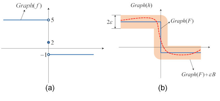
has ={0}0\mathcal{M}=\{0\} which determines on \mathbb{R} the continuity sub-domains 𝒟1=(,0]subscript𝒟10\mathcal{D}_{1}=(-\infty,0] and 𝒟2=[0,)subscript𝒟20\mathcal{D}_{2}=[0,\infty). The graph is plotted in Fig. 1a.

The form of f𝑓f, given by (1), appears in the great majority of nonlinear piece-wise continuous systems of fractional or integer order, which are modeled by the following Initial Value Problem (IVP)

Dqx(t)=f(x(t)):=g(x(t))+Kx(t)+A(x(t))s(x(t)),x(0)=x0,tI=[0,).formulae-sequencesuperscriptsubscript𝐷𝑞𝑥𝑡𝑓𝑥𝑡assign𝑔𝑥𝑡𝐾𝑥𝑡𝐴𝑥𝑡𝑠𝑥𝑡formulae-sequence𝑥0subscript𝑥0𝑡𝐼0D_{*}^{q}x(t)=f(x(t)):=g(x(t))+Kx(t)+A(x(t))s(x(t)),~{}~{}~{}x(0)=x_{0},~{}~{}~{}t\in I=[0,\infty). (3)

In this paper, Dqsuperscriptsubscript𝐷𝑞D_{*}^{q}, with q=(q1,q2,,qn)𝑞subscript𝑞1subscript𝑞2subscript𝑞𝑛q=(q_{1},q_{2},...,q_{n}), 0<qi10subscript𝑞𝑖10<q_{i}\leq 1, i=1,2,,n𝑖12𝑛i=1,2,...,n (q=1𝑞1q=1 for the integer order), denotes the commonly used operator in fractional calculus: Caputo’s differential operator of order q𝑞q (called also smooth fractional derivative with starting point 0)[8, 9, 10]

Dqx(t)=1Γ(1q)0t(tτ)qddtx(τ)𝑑τ,superscriptsubscript𝐷𝑞𝑥𝑡1Γ1𝑞superscriptsubscript0𝑡superscript𝑡𝜏𝑞𝑑𝑑𝑡𝑥𝜏differential-d𝜏D_{*}^{q}x(t)=\frac{1}{\Gamma(1-q)}\int_{0}^{t}(t-\tau)^{-q}\frac{d}{dt}x(\tau)d\tau,

where ΓΓ\Gamma is the Euler’s Gamma function

Γ(z)=0ttz1et𝑑t,z,Re(z)>0.formulae-sequenceΓ𝑧superscriptsubscript0𝑡superscript𝑡𝑧1superscript𝑒𝑡differential-d𝑡formulae-sequence𝑧𝑅𝑒𝑧0\Gamma(z)=\int_{0}^{t}t^{z-1}e^{-t}dt,~{}~{}~{}z\in\mathbb{C},~{}~{}Re(z)>0.

We consider in this paper 3superscript3\mathbb{R}^{3} examples. For example, the fractional variant of the piece-wise Chen system [11]

Dq1x1=a(x2x1),Dq2x2=(cax3)sgn(x1)+cdx2,Dq3x3=x1sgn(x2)bx3.superscriptsubscript𝐷subscript𝑞1subscript𝑥1𝑎subscript𝑥2subscript𝑥1superscriptsubscript𝐷subscript𝑞2subscript𝑥2𝑐𝑎subscript𝑥3𝑠𝑔𝑛subscript𝑥1𝑐𝑑subscript𝑥2superscriptsubscript𝐷subscript𝑞3subscript𝑥3subscript𝑥1𝑠𝑔𝑛subscript𝑥2𝑏subscript𝑥3\begin{array}[]{l}D_{\ast}^{q_{1}}x_{1}=a\left(x_{2}-x_{1}\right),\\ D_{\ast}^{q_{2}}x_{2}=\left(c-a-x_{3}\right)sgn(x_{1})+cdx_{2},\\ D_{\ast}^{q_{3}}x_{3}=x_{1}sgn(x_{2})-bx_{3}.\end{array} (4)

with a=1.18𝑎1.18a=1.18, b=0.16𝑏0.16b=0.16, c=1.2𝑐1.2c=1.2, d=0.1𝑑0.1d=0.1 and the fractional-order (q1,q2,q3)subscript𝑞1subscript𝑞2subscript𝑞3(q_{1},q_{2},q_{3}), has g(x)=(0,0,0)T𝑔𝑥superscript000𝑇g(x)=\left(0,0,0\right)^{T} (i.e. f𝑓f in this case is piece-wise linear), s(x)=(sgn(x1),sgn(x2),sgn(x3))T𝑠𝑥superscript𝑠𝑔𝑛subscript𝑥1𝑠𝑔𝑛subscript𝑥2𝑠𝑔𝑛subscript𝑥3𝑇s(x)=(sgn(x_{1}),sgn(x_{2}),\allowbreak sgn(x_{3}))^{T} and

K=(aa00cd000b),𝐾𝑎𝑎00𝑐𝑑000𝑏K=\left(\begin{array}[]{ccc}-a&a&0\\ 0&cd&0\\ 0&0&-b\end{array}\right),

and

A(x)=(000cax3000x10).𝐴𝑥000𝑐𝑎subscript𝑥3000subscript𝑥10A(x)=\left(\begin{array}[]{ccc}0&0&0\\ c-a-x_{3}&0&0\\ 0&x_{1}&0\end{array}\right).

As in most practical examples, the use of Caputo derivative in the IVP (3) is fully justified since in these problems we need physically interpretable initial conditions, or Caputo derivative satisfies these demands, by avoiding the expression of initial conditions with fractional derivatives [4]. Accordingly, the initial condition in (3), can be considered in the standard form x(0)=x0𝑥0subscript𝑥0x(0)=x_{0}.

To overcome the discontinuity impediment, we shall use Filippov’s approach [1]. This technique targets the piece-wise constant functions s𝑠s, and converts them in set-valued functions. Next, via Cellina’s Theorem [2, 3], the set-valued functions are continuously approximated in small neighborhoods of underlying set-valued functions.

The results are valid for a large class such as Heaviside function H𝐻H, rectangular function (as difference of two Heaviside functions), or signum, one of the most encountered functions in practical applications.

The paper is organize as follows: Section 2 deals with the approximation of f𝑓f defined by (1) and shows how the IVP (3) can be transformed into a continuous single valued problem. In Section 3 the asymptotically synchronization of piece-wise continuous systems of fractional-order is investigated and the necessary condition for chaotic behavior of these system is presented. In Section 4 the asymptotically synchronization is applied to three piece-wise continuous systems of fractional-order: Chen’s system, Sprott’s system and Shimizu- Morioka’s system. Appendix includes proofs and results utilized in the paper.

2 Continuous approximation of f𝑓f

In this section we prove that the considered class of piece-wise continuous functions defined in (1), can be approximated as closely as desired with continuous functions. First, the piece-wise continuous function f𝑓f will be transformed into a set-valued function, which will be approximated with continuous functions. For this purpose, we will choose the way proposed by Fillipov in [1], namely the Filippov regularization. Thus, the discontinuous function f𝑓f is transformed into a convex set-valued function F𝐹F into the set of all subsets of nsuperscript𝑛\mathbb{R}^{n}, F:nn:𝐹superscript𝑛superscript𝑛F:\mathbb{R}^{n}\rightrightarrows\mathbb{R}^{n}. One of the simplest expressions for F𝐹F, is [1, 2, 3]

F(x)=ε>0μ()=0conv¯(f(zn:|zx|ε\)).F(x)=\bigcap_{\varepsilon>0}\bigcap_{\mu(\mathcal{M})=0}\overline{conv}(f({z\in\mathbb{R}^{n}:|z-x|\leq\varepsilon}\backslash\mathcal{M})). (5)

F(x)𝐹𝑥F(x) is the convex hull of f(x)𝑓𝑥f(x), μ𝜇\mu being the Lebesgue measure and ε𝜀\varepsilon the radius of the ball centered in x𝑥x. At the points where f𝑓f is continuous, F(x)𝐹𝑥F(x) consists of one single point, which coincides with the value of f𝑓f at this point (i.e. we get back f(x)𝑓𝑥f(x) as the right hand side: F(x)={f(x)}𝐹𝑥𝑓𝑥F(x)=\{f(x)\}). In the points belonging to \mathcal{M}, F(x)𝐹𝑥F(x) is given by (5).

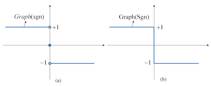
If the piece-wise-constant functions sisubscript𝑠𝑖s_{i} are sgn𝑠𝑔𝑛sgn functions, their set-valued form, obtained with Filippov regularization, denoted by Sgn::𝑆𝑔𝑛Sgn:\mathbb{R}\rightrightarrows\mathbb{R}, is defined as follows (see Fig. 2a) before regularization and Fig. 2b) after regularization)

Sgn(x)={{1},x<0,[1,1],x=0,{+1},x>0.𝑆𝑔𝑛𝑥cases1𝑥011𝑥01𝑥0Sgn(x)=\left\{\begin{array}[]{cc}\{-1\},&x<0,\\ [-1,1],&x=0,\\ \{+1\},&x>0.\end{array}\right. (6)

By applying the Filippov regularization to f𝑓f, one obtains the following set-valued function

F(x)=g(x)+Kx+A(x)S(x),𝐹𝑥𝑔𝑥𝐾𝑥𝐴𝑥𝑆𝑥F(x)=g(x)+Kx+A(x)S(x), (7)

with

S(x)=(S1(x1),S2(x2),,Sn(xn))T,𝑆𝑥superscriptsubscript𝑆1subscript𝑥1subscript𝑆2subscript𝑥2subscript𝑆𝑛subscript𝑥𝑛𝑇S(x)=(S_{1}(x_{1}),S_{2}(x_{2}),...,S_{n}(x_{n}))^{T}, (8)

Si::subscript𝑆𝑖S_{i}:\mathbb{R}\rightarrow\mathbb{R} being the set-valued variants of sisubscript𝑠𝑖s_{i}, i=1,2,,n𝑖12𝑛i=1,2,...,n (Sgn(xi)𝑆𝑔𝑛subscript𝑥𝑖Sgn(x_{i}) in the usual case of sgn(xi)𝑠𝑔𝑛subscript𝑥𝑖sgn(x_{i})).

For example, the graph of the set-valued variant of f𝑓f defined in (2) is plotted in Fig. 1b.

The notions and results presented next are considered in \mathbb{R}, but they are also valid in the general case nsuperscript𝑛\mathbb{R}^{n}, n>1𝑛1n>1. Let a set-valued function F::𝐹F:\mathbb{R}\rightrightarrows\mathbb{R}.

A set-valued function F𝐹F can be characterized by its graph

Graph(F):={(x,y)×,yF(x)}.assign𝐺𝑟𝑎𝑝𝐹formulae-sequence𝑥𝑦𝑦𝐹𝑥Graph(F):=\{(x,y)\in\mathbb{R}\times\mathbb{R},~{}y\in F(x)\}.
Remark 1.

Due to the symmetric interpretation of a set-valued function as a graph (see e.g. [2]) we shall say that a set-valued function satisfies a property if and only if its graph satisfies it. For instance, a set-valued function is said to be closed if and only if its graph is closed.

Definition 2.

A set-valued function F𝐹F is upper semicontinous (u.s.c.) at x0superscript𝑥0x^{0}\in\mathbb{R}, if for any open set E𝐸E containing F(x0)𝐹superscript𝑥0F(x^{0}), there exists a neighborhood A𝐴A of x0superscript𝑥0x^{0} such that F(A)B𝐹𝐴𝐵F(A)\in B.

We say that F𝐹F is u.s.c. if it is so at every x0superscript𝑥0x^{0}\in\mathbb{R}.

U.s.c., which is a basic property, practically means that the graph of F𝐹F is closed.

Definition 3.

A single-valued function h::h:\mathbb{R}\rightarrow\mathbb{R} is called an approximation (selection) of the set-valued function F𝐹F if

x,h(x)F(x).formulae-sequencefor-all𝑥𝑥𝐹𝑥\forall x\in\mathbb{R},~{}~{}h(x)\in F(x).

Generally, a set-valued function admits (infinitely) many approximations (see Fig. 1b for the case of function defined in (2)).

As proved in [12], the set-valued functions Sisubscript𝑆𝑖S_{i}, i=1,2,,n𝑖12𝑛i=1,2,...,n, can be approximated due to the Approximate Theorem, called also Cellina’s Theorem (Appendix) which states that a set-valued function F𝐹F, with closed graph and convex values, admits continuous approximations. This result is assured by the following lemma

Lemma 1.

For every ε>0𝜀0\varepsilon>0, the set-valued functions Sisubscript𝑆𝑖S_{i}, i=1,2,,n𝑖12𝑛i=1,2,...,n admit continuous approximations in the ε𝜀\varepsilon-neighborhood of Sisubscript𝑆𝑖S_{i}.

Proof.

Sisubscript𝑆𝑖S_{i}, for i=1,2,,n𝑖12𝑛i=1,2,...,n, are convex u.s.c. (see e.g. the Remark in [1] p. 43 or the Example in [3] p. 39 for u.s.c.) and, via Remark 1, are non-empty closed valued functions. Therefore, they verifies Cellina’s Theorem which guaranties the existence of continuous approximations on \mathbb{R}. ∎

Notation 4.

Let denote by s~i::subscript~𝑠𝑖\widetilde{s}_{i}:\mathbb{R}\rightarrow\mathbb{R} the approximations of Sisubscript𝑆𝑖S_{i}.

For the sake of simplicity, for each component s~i(xi)subscript~𝑠𝑖subscript𝑥𝑖\widetilde{s}_{i}(x_{i}), i=1,2,,n𝑖12𝑛i=1,2,...,n, εisubscript𝜀𝑖\varepsilon_{i} will be considered as having the same value.

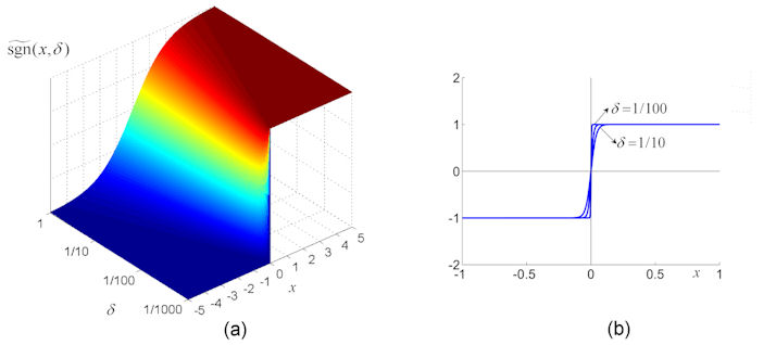
Some of the best candidates for s~~𝑠\widetilde{s} are the sigmoid functions, since they provide the required flexibility and to which the abruptness of the discontinuity can be easily modified. For S(x)=Sgn(x)𝑆𝑥𝑆𝑔𝑛𝑥S(x)=Sgn(x), one of the most utilized sigmoid approximations is the following function sgn~~𝑠𝑔𝑛\widetilde{sgn}222The class of sigmoid functions includes for example the ordinary arctangent such as 2πarctanxε2𝜋𝑎𝑟𝑐𝑡𝑎𝑛𝑥𝜀\frac{2}{\pi}arctan\frac{x}{\varepsilon}, the hyperbolic tangent, the error function, the logistic function, algebraic functions like xϵ+x2𝑥italic-ϵsuperscript𝑥2\frac{x}{\sqrt{\epsilon+x^{2}}}, and so on.

sgn~(x)=21+exδ1Sgn(x),~𝑠𝑔𝑛𝑥21superscript𝑒𝑥𝛿1𝑆𝑔𝑛𝑥\widetilde{sgn}(x)=\frac{2}{1+e^{-\frac{x}{\delta}}}-1\approx Sgn(x), (9)

where δ𝛿\delta is a positive parameter which controls the slope in the neighborhood of the discontinuity x=0𝑥0x=0 (Fig. 3a and Fig. 3b).

Summarizing, we can enounce the following result, which assures the possibility to approximate continuously f𝑓f

Theorem 5.

Let f𝑓f defined by (1). If g𝑔g is continuous, then there exist continuous approximations of f𝑓f, f~:nn:~𝑓superscript𝑛superscript𝑛\tilde{f}:\mathbb{R}^{n}\rightarrow\mathbb{R}^{n}

f~(x)=g(x)+Kx+A(x)s~(x)f(x).~𝑓𝑥𝑔𝑥𝐾𝑥𝐴𝑥~𝑠𝑥𝑓𝑥\tilde{f}(x)=g(x)+Kx+A(x)\widetilde{s}(x)\approx f(x). (10)

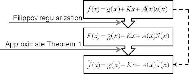
Specifically, Theorem 5 actually means that the considered function f𝑓f can be approximated simply by replacing s𝑠s with s~~𝑠\tilde{s} (dotted line in sketch in Fig. 4). For example, f𝑓f defined by (2), can be approximated as follows

f~(x)=23sgn~(x)=23(21+exδ1).~𝑓𝑥23~𝑠𝑔𝑛𝑥2321superscript𝑒𝑥𝛿1\tilde{f}(x)=2-3\widetilde{sgn}(x)=2-3\left(\frac{2}{1+e^{-\frac{x}{\delta}}}-1\right). (11)

Theorem 5 states that systems modeled by the IVP (3), can be continuously approximated by the following continuous IVP

Dq(x)=f~(x),x(0)=x0,formulae-sequencesuperscriptsubscript𝐷𝑞𝑥~𝑓𝑥𝑥0subscript𝑥0D_{*}^{q}(x)=\tilde{f}(x),~{}~{}~{}x(0)=x_{0},

with f~~𝑓\tilde{f} defined by (10).

3 Synchronization

Once we proved that systems modeled by (3) can be continuously approximated, they can be synchronized via any kind of synchronization schemes for continuous systems. In this paper we consider the synchronization in coupled chaotic system via master-slave configuration.

As known, a linear autonomous system of fractional-order is asymptotically stable if his zero (equilibrium) point is asymptotically stable.

The computation of the Jacobian requires the following assumption

(H2) Function g𝑔g in (1) is suppose to be differentiable on nsuperscript𝑛\mathbb{R}^{n}.

Since the discontinuous functions appearing in the considered examples are sgn𝑠𝑔𝑛sgn, next we study some properties of this function and its approximations.

Let Xsuperscript𝑋X^{*} and X~superscript~𝑋\tilde{X}^{*} the equilibrium points of f𝑓f and f~~𝑓\tilde{f} respectively, and J𝐽J and J~~𝐽\tilde{J} the related Jacobians.

Property 1 For every δ>0𝛿0\delta>0, there exists a small neighborhood of \mathcal{M}, 𝒱𝒱\mathcal{V}, depending on δ𝛿\delta, such that X~Xsuperscript~𝑋superscript𝑋\tilde{X}^{*}\approx X^{*} for x𝒱𝑥𝒱x\not\in\mathcal{V}.

See the proof in Appendix.

Remark 2.

As known, the error of ABM method utilized in this paper to integrate the fractional DE, is of order O(hp)𝑂superscript𝑝O(h^{p}) [4] with p=min(2,1+qmin)𝑝𝑚𝑖𝑛21subscript𝑞𝑚𝑖𝑛p=min(2,1+q_{min}). For our step size h=0.0050.005h=0.005, this error is of order of 1e51𝑒51e-5. On the other side, in order to ensure the validity of Property 3 for a large class of systems (3), the size of 𝒱𝒱\mathcal{V} must be smaller than hpsuperscript𝑝h^{p}. δ=1/100000𝛿1100000\delta=1/100000, proves to be an acceptable compromise between the numerical accuracy and computer precision and also assures the requirements for Property 3. For this choice, 𝒱=(1.589e4,1.589e4)𝒱1.589𝑒41.589𝑒4\mathcal{V}=(-1.589e-4,1.589e-4) and for x𝒱𝑥𝒱x\not\in\mathcal{V}, the difference between sgn~~𝑠𝑔𝑛\widetilde{sgn} and the branch ±1plus-or-minus1\pm 1 of the function sgn𝑠𝑔𝑛sgn is of order of 1e71𝑒71e-7. In all studied examples, X(X~)superscript𝑋superscript~𝑋X^{*}(\tilde{X}^{*}) are situated outside of these neighborhoods.

Regarding the size of δ𝛿\delta the following hypothesis is considered

(H3) In this paper we chosen δ=1/100000𝛿1100000\delta=1/100000.

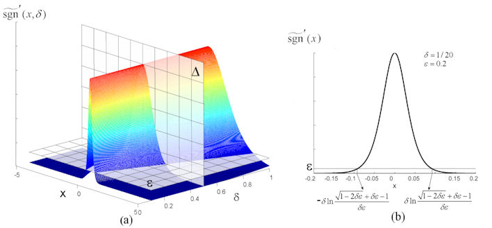
For the derivative ddxsgn~𝑑𝑑𝑥~𝑠𝑔𝑛\frac{d}{dx}\widetilde{sgn} (plotted as function on δ𝛿\delta in Fig. 5a), the following property holds Property 2 Assume (H2). For every δ>0𝛿0\delta>0, there exists a neighborhood of x=0𝑥0x=0, 𝒱𝒱\mathcal{V}, depending on δ𝛿\delta such that J~|X~J|Xevaluated-at~𝐽superscript~𝑋evaluated-at𝐽superscript𝑋\tilde{J}|_{\widetilde{X}^{*}}\approx J|_{X^{*}}, for x𝒱𝑥𝒱x\not\in\mathcal{V}.

See the proof in Appendix.

Let consider the following piece-wise continuous master system of fractional-order

Dqx=f(x):=g(x)+Kx+A(x)s(x),x(0)=x0,formulae-sequencesubscriptsuperscript𝐷𝑞𝑥𝑓𝑥assign𝑔𝑥𝐾𝑥𝐴𝑥𝑠𝑥𝑥0subscript𝑥0D^{q}_{*}x=f(x):=g(x)+Kx+A(x)s(x),~{}~{}~{}x(0)=x_{0}, (12)

and the slave system

Dqy=f(y)+u:=g(y)+Ky+A(y)s(y)+u,y(0)=y0,formulae-sequencesubscriptsuperscript𝐷𝑞𝑦𝑓𝑦𝑢assign𝑔𝑦𝐾𝑦𝐴𝑦𝑠𝑦𝑢𝑦0subscript𝑦0D^{q}_{*}y=f(y)+u:=g(y)+Ky+A(y)s(y)+u,~{}~{}~{}y(0)=y_{0}, (13)

where un𝑢superscript𝑛u\in\mathbb{R}^{n} is the control designed such as the state of the slave system (13) evolves as the states of the master system (12).

After continuous approximation, the master system becomes

Dqx=f~(x):=g(x)+Kx+A(x)s~(x),x0=x(0),formulae-sequencesubscriptsuperscript𝐷𝑞𝑥~𝑓𝑥assign𝑔𝑥𝐾𝑥𝐴𝑥~𝑠𝑥subscript𝑥0𝑥0D^{q}_{*}x=\tilde{f}(x):=g(x)+Kx+A(x)\tilde{s}(x),~{}~{}~{}x_{0}=x(0), (14)

and the slave system

Dqy=f~(y)+u:=g(y)+Ky+A(y)s~(y)+u,y0=y(0).formulae-sequencesubscriptsuperscript𝐷𝑞𝑦~𝑓𝑦𝑢assign𝑔𝑦𝐾𝑦𝐴𝑦~𝑠𝑦𝑢subscript𝑦0𝑦0D^{q}_{*}y=\tilde{f}(y)+u:=g(y)+Ky+A(y)\tilde{s}(y)+u,~{}~{}~{}y_{0}=y(0). (15)

The utilized active control method requires to design un𝑢superscript𝑛u\in\mathbb{R}^{n} such as the error, defined as e=yx𝑒𝑦𝑥e=y-x, tends asymptotically to zero: limte(t)=0𝑡norm𝑒𝑡0\underset{t\rightarrow\infty}{\lim}||e(t)||=0 (||||||\cdot|| being the Euclidean norm). Thus, the error dynamical system is obtained by subtracting (14) from (15)

Dqe=g(y)g(x)+Ke+A(y)s~(y)A(x)s~(x)+u,e(0)=y(0)x(0).formulae-sequencesubscriptsuperscript𝐷𝑞𝑒𝑔𝑦𝑔𝑥𝐾𝑒𝐴𝑦~𝑠𝑦𝐴𝑥~𝑠𝑥𝑢𝑒0𝑦0𝑥0D^{q}_{*}e=g(y)-g(x)+Ke+A(y)\tilde{s}(y)-A(x)\tilde{s}(x)+u,~{}~{}~{}e(0)=y(0)-x(0). (16)

and the asymptotically synchronization transforms into asymptotically stability of the zero equilibrium point of (16). For this purpose, u𝑢u has to be defined such as the error system becomes an asymptotically stable linear system. The usual choice for the active control is

u=g(y)+g(x)A(y)s~(y)+A(x)s~(x)+v,𝑢𝑔𝑦𝑔𝑥𝐴𝑦~𝑠𝑦𝐴𝑥~𝑠𝑥𝑣u=-g(y)+g(x)-A(y)\widetilde{s}(y)+A(x)\widetilde{s}(x)+v,

with vn𝑣superscript𝑛v\in\mathbb{R}^{n}, v=Me𝑣𝑀𝑒v=Me, where M𝑀M is some real square matrix MRn×n𝑀superscript𝑅𝑛𝑛M\in R^{n\times n}, which can be chosen in many possible ways. Thus, by replacing u𝑢u in (16), the error system becomes a linear system

Dqe=Ee,e(0)=y(0)x(0),formulae-sequencesubscriptsuperscript𝐷𝑞𝑒𝐸𝑒𝑒0𝑦0𝑥0D^{q}_{*}e=Ee,~{}~{}~{}e(0)=y(0)-x(0), (17)

with E=M+K𝐸𝑀𝐾E=M+K.

Theorem 6.

The piece-wise continuous master-slave system (12)-(13) asymptotically synchronizes if and only if:

  • a.

    for the commensurate case, all eigenvalues λ𝜆\lambda of E𝐸E, verify the condition

    |arg(λ)|>qπ/2;𝑎𝑟𝑔𝜆𝑞𝜋2|arg(\lambda)|>q\pi/2; (18)
  • b.

    for the incommensurate case qi=ki/mi<1subscript𝑞𝑖subscript𝑘𝑖subscript𝑚𝑖1q_{i}=k_{i}/m_{i}<1, kisubscript𝑘𝑖k_{i}, misubscript𝑚𝑖m_{i}\in\mathbb{N}, mi0subscript𝑚𝑖0m_{i}\neq 0, for i=1,2,,n𝑖12𝑛i=1,2,...,n, kisubscript𝑘𝑖k_{i}, misubscript𝑚𝑖m_{i} being coprime positive integers, (ki,mi)=1subscript𝑘𝑖subscript𝑚𝑖1(k_{i},m_{i})=1, all the roots of the characteristic equation

    P(λ):=det(diag[λmq1,λmq2,,λmqn]E)=0,assign𝑃𝜆𝑑𝑒𝑡𝑑𝑖𝑎𝑔superscript𝜆𝑚subscript𝑞1superscript𝜆𝑚subscript𝑞2superscript𝜆𝑚subscript𝑞𝑛𝐸0P(\lambda):=det(diag[\lambda^{mq_{1}},\lambda^{mq_{2}},...,\lambda^{mq_{n}}]-E)=0, (19)

    with m𝑚m the least common multiple of the denominators misubscript𝑚𝑖m_{i} verify the condition

    |arg(λ)|>π/2m.𝑎𝑟𝑔𝜆𝜋2𝑚|arg(\lambda)|>\pi/2m. (20)
Proof.

Under the assumptions given by Properties 3 and Property 3, the master and the slave systems transform into continuous systems of fractional-order and the proof follows the same steps such as the proof for original theorems for continuous systems (see [13, 14] for commensurate and incommensurate cases respectively). ∎

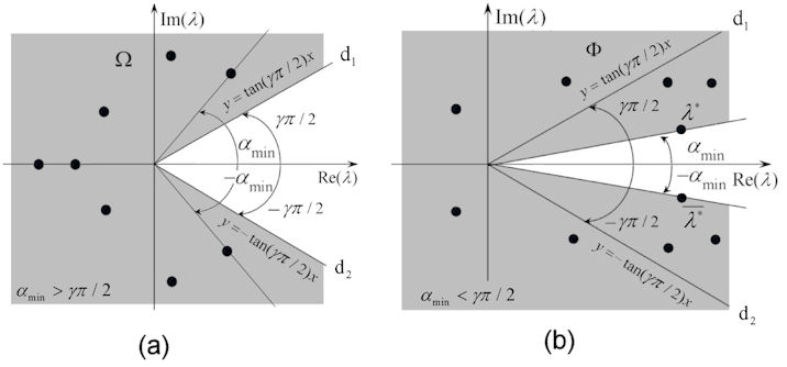
Summarizing, if we denote with ΛΛ\Lambda the spectrum of the eigenvalues of E𝐸E or of the roots of (19), and with αmin=min{|arg(Λ)}\alpha_{min}=min\{|arg(\Lambda)\}, the sufficient and necessary asymptotically synchronization conditions (18) and (20) can be written as follows

αmin>γπ/2,subscript𝛼𝑚𝑖𝑛𝛾𝜋2\alpha_{min}>\gamma\pi/2, (21)

where γ=q𝛾𝑞\gamma=q for the commensurate case, and γ=1/m𝛾1𝑚\gamma=1/m in the case of incommensurate case, or ΛΛ\Lambda is included in the domain ΩΩ\Omega defined as follows (Fig. 6a)

ΛΩ={λ,|arg{λ}|>γπ/2}.ΛΩformulae-sequence𝜆𝜆𝛾𝜋2\Lambda\subset\Omega=\{\lambda\in\mathbb{C},|\arg\{\lambda\}|>\gamma\pi/2\}.
Remark 3.
  • i)

    Relations (18), (20) or (21) with """""\geq" instead "<""""<", mean that there are λisubscript𝜆𝑖\lambda_{i} situated on the separatrices d1,2subscript𝑑12d_{1,2} having the equations ±tan(γπ/2)plus-or-minus𝑡𝑎𝑛𝛾𝜋2\pm tan(\gamma\pi/2) (Fig. 6). If those eigenvalues (or roots) situated on d1,2subscript𝑑12d_{1,2} (for example the points λsuperscript𝜆\lambda^{*} and λ¯superscript¯𝜆\bar{\lambda}^{*} in Fig. 6b which satisfy the equality), have geometric multiplicity of one, then the synchronization is only stable and not asymptotical stable.333The geometric multiplicity represents the dimension of the eigenspace of eigenvalues.

  • ii)

    It is to note that arg𝑎𝑟𝑔arg should be not considered arctan𝑎𝑟𝑐𝑡𝑎𝑛arctan function, since arctan(π/2,π/2)𝑎𝑟𝑐𝑡𝑎𝑛𝜋2𝜋2arctan\in(-\pi/2,\pi/2), while arg[π,π]𝑎𝑟𝑔𝜋𝜋arg\in[-\pi,\pi]. A possible choice is the function atan2𝑎𝑡𝑎𝑛2atan2 implemented in some software packages or, for example, the formulae arg(z)=arctan(y/x)+pi/2sign(y)(1sign(x))𝑎𝑟𝑔𝑧𝑎𝑟𝑐𝑡𝑎𝑛𝑦𝑥𝑝𝑖2𝑠𝑖𝑔𝑛𝑦1𝑠𝑖𝑔𝑛𝑥arg(z)=arctan(y/x)+pi/2sign\\ (y)(1-sign(x)), or 2arctan(x2+y2xy)2𝑎𝑟𝑐𝑡𝑎𝑛superscript𝑥2superscript𝑦2𝑥𝑦2arctan(\frac{\sqrt{x^{2}+y^{2}}-x}{y}), where z=x+iy𝑧𝑥𝑖𝑦z=x+iy.

Chaotic piece-wise continuous systems of fractional-order

Since in this paper the synchronization deals with chaotic motions, we shall study computationally the existence of chaotic behaviors for the considered examples, beside a necessary criterion for chaos existence in fractional-order nonlinear systems, derived from the Stability Theorem 6.

We do not consider here the qualitative aspects of the equilibrium points but only the necessary condition for chaos and numerical evidences of chaotic motions (see e.g. [15] for a study on the number of saddle points, underlying eigenvalues, one-scroll, double-scroll).

Hereafter, it is supposed that the determination of X~superscript~𝑋\tilde{X}^{*} and J~~𝐽\tilde{J}, are assured by Properties 3 and 3.

The utilized numerical method is the Adamas-Bashforth-Moulton variant, proposed by Kai et al in [4], and the utilized step size h=0.0050.005h=0.005.

The trajectories corners which can be seen in phase plots and time series, are typical to discontinuous systems [6, 7].

Let consider an approximated system of fractional-order (14), with X~superscript~𝑋\tilde{X}^{*} the equilibrium points and J~~𝐽\tilde{J} the Jacobian matrix.

The condition necessary for chaotic motion related to one of the equilibria Xsuperscript𝑋X^{*}, is [16]

αminγπ/2,subscript𝛼𝑚𝑖𝑛𝛾𝜋2\alpha_{min}\leq\gamma\pi/2, (22)

or ΛΦ={λ,|arg(λ)|αmin,αminγπ/2}ΛΦformulae-sequence𝜆formulae-sequence𝑎𝑟𝑔𝜆subscript𝛼𝑚𝑖𝑛subscript𝛼𝑚𝑖𝑛𝛾𝜋2\Lambda\subset\Phi=\{\lambda\in\mathbb{C},|arg(\lambda)|\geq\alpha_{min},~{}\alpha_{min}\leq\gamma\pi/2\} (Fig. 6b).

In this case, αminsubscript𝛼𝑚𝑖𝑛\alpha_{min} is determined for the Jacobian J~Xsubscript~𝐽superscript𝑋\tilde{J}_{X^{*}}, or for the roots of the characteristic equation

P(λ):=det(diag[λmq1,λmq2,,λmqn]J~X)=0assign𝑃𝜆𝑑𝑒𝑡𝑑𝑖𝑎𝑔superscript𝜆𝑚subscript𝑞1superscript𝜆𝑚subscript𝑞2superscript𝜆𝑚subscript𝑞𝑛subscript~𝐽superscript𝑋0P(\lambda):=det(diag[\lambda^{mq_{1}},\lambda^{mq_{2}},...,\lambda^{mq_{n}}]-\tilde{J}_{X^{*}})=0 (23)

Even (22) is only a necessary condition for chaos, it is useful to find the minimum commensurate order q𝑞q for system (3) to remain chaotic. Thus, once we find ΛΛ\Lambda and αminsubscript𝛼𝑚𝑖𝑛\alpha_{min}, by setting in (22) γ=q𝛾𝑞\gamma=q, the values of q𝑞q from which chaos might appear are

q>qmin=2παmin.𝑞subscript𝑞𝑚𝑖𝑛2𝜋subscript𝛼𝑚𝑖𝑛q>q_{min}=\frac{2}{\pi}\alpha_{min}. (24)

For example let us consider the Chen’s system (4)

Dq1x1=a(x2x1),Dq2x2=(cax3)sgn(x1)+cdx2,Dq3x3=x1sgn(x2)bx3.superscriptsubscript𝐷subscript𝑞1subscript𝑥1𝑎subscript𝑥2subscript𝑥1superscriptsubscript𝐷subscript𝑞2subscript𝑥2𝑐𝑎subscript𝑥3𝑠𝑔𝑛subscript𝑥1𝑐𝑑subscript𝑥2superscriptsubscript𝐷subscript𝑞3subscript𝑥3subscript𝑥1𝑠𝑔𝑛subscript𝑥2𝑏subscript𝑥3\begin{array}[]{l}D_{\ast}^{q_{1}}x_{1}=a\left(x_{2}-x_{1}\right),\\ D_{\ast}^{q_{2}}x_{2}=\left(c-a-x_{3}\right)sgn(x_{1})+cdx_{2},\\ D_{\ast}^{q_{3}}x_{3}=x_{1}sgn(x_{2})-bx_{3}.\end{array} (25)

and his the continuous approximation.

Dq1x1=a(x2x1),Dq2x2=(cax3)sgn~(x1)+cdx2,Dq3x3=x1sgn~(x2)bx3.superscriptsubscript𝐷subscript𝑞1subscript𝑥1𝑎subscript𝑥2subscript𝑥1superscriptsubscript𝐷subscript𝑞2subscript𝑥2𝑐𝑎subscript𝑥3~𝑠𝑔𝑛subscript𝑥1𝑐𝑑subscript𝑥2superscriptsubscript𝐷subscript𝑞3subscript𝑥3subscript𝑥1~𝑠𝑔𝑛subscript𝑥2𝑏subscript𝑥3\begin{array}[]{l}D_{\ast}^{q_{1}}x_{1}=a\left(x_{2}-x_{1}\right),\\ D_{\ast}^{q_{2}}x_{2}=\left(c-a-x_{3}\right)\widetilde{sgn}(x_{1})+cdx_{2},\\ D_{\ast}^{q_{3}}x_{3}=x_{1}\widetilde{sgn}(x_{2})-bx_{3}.\end{array} (26)

Beside the origin, the system has two other equilibria X~1,2=(±0.003,±0.003,0.020)subscriptsuperscript~𝑋12plus-or-minus0.003plus-or-minus0.0030.020\tilde{X}^{*}_{1,2}=(\pm 0.003,\pm 0.003,0.020) and the Jacobian

J~=(aa00cdsgn(x1)sgn(x2)0b)X~1,2.~𝐽subscript𝑎𝑎00𝑐𝑑𝑠𝑔𝑛subscript𝑥1𝑠𝑔𝑛subscript𝑥20𝑏subscriptsuperscript~𝑋12\tilde{J}=\left(\begin{array}[]{ccc}-a&a&0\\ 0&cd&-sgn(x_{1})\\ sgn(x_{2})&0&-b\end{array}\right)_{\tilde{X}^{\ast}_{1,2}}.

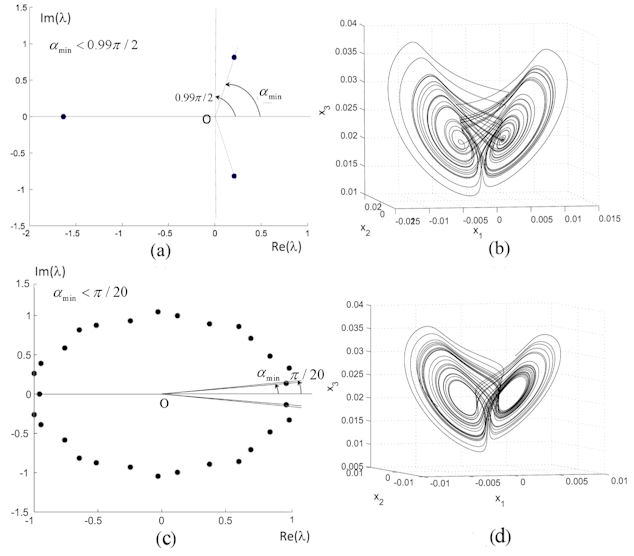
The eigenvalues at X~1,2superscriptsubscript~𝑋12\tilde{X}_{1,2}^{*} are Λ=(1.636,0.208+0.815i,0.2080.815i)Λ1.6360.2080.815𝑖0.2080.815𝑖\Lambda=(-1.636,0.208+0.815i,\\ 0.208-0.815i), arg{Λ}={3.141,1.321,1.321}𝑎𝑟𝑔Λ3.1411.3211.321arg\{\Lambda\}=\{3.141,1.321,-1.321\}.

Let consider the case of X~1=(0.003,0.003,0.020)subscriptsuperscript~𝑋10.0030.0030.020\tilde{X}^{*}_{1}=(0.003,0.003,0.020), similar results being obtained for X~2subscriptsuperscript~𝑋2\tilde{X}^{*}_{2}.

Commensurate case

: q=0.99𝑞0.99q=0.99. Condition (22) is verified: αmin=1.321<1.555=0.99π/2subscript𝛼𝑚𝑖𝑛1.3211.5550.99𝜋2\alpha_{min}=1.321<1.555=0.99\pi/2, ΛΦΛΦ\Lambda\subset\Phi (Fig. 7a), and for this value of q𝑞q, the system is chaotic (Fig. 7b).

The minim commensurate value of q𝑞q to have chaotic behavior is, via (24), q>qmin=2αmin/π=0.841𝑞subscript𝑞𝑚𝑖𝑛2subscript𝛼𝑚𝑖𝑛𝜋0.841q>q_{min}=2\alpha_{min}/\pi=0.841.

Incommensurate case

: q=(1,0.9,1)𝑞10.91q=(1,0.9,1). The characteristic polynomial (23) is

λ293/25λ20+67/50λ19201/1250λ10+118/625λ9+36167/31250.superscript𝜆29325superscript𝜆206750superscript𝜆192011250superscript𝜆10118625superscript𝜆93616731250\lambda^{29}-3/25\lambda^{20}+67/50\lambda^{19}-201/1250\lambda^{10}+118/625\lambda^{9}+36167/31250.

Here, m=10𝑚10m=10, γ=1/10𝛾110\gamma=1/10 and αmin=0.138<0.157=π/20subscript𝛼𝑚𝑖𝑛0.1380.157𝜋20\alpha_{min}=0.138<0.157=\pi/20. Therefore condition (22) is verified and ΛΦΛΦ\Lambda\subset\Phi (Fig. 7c). The system behaves chaotic (Fig. 7d).

4 Applications

In this section we synchronize three-dimensional systems: Sprott’s systems, Chen’s systems and Shimizu- Morioka’s systems, after which, we synchronize two different systems: Sprott’s and Chen’s systems.

For all numerical experiments, beside phase plots (where the trajectories of the master and slave systems are overplotted) and time series, we calculated the Hausdorff distance dHsubscript𝑑𝐻d_{H} (Appendix). After few hundreds steps have been neglected, dHsubscript𝑑𝐻d_{H} is of order of 1e51𝑒51e-5. Time series details (for t[0,20]𝑡020t\in[0,20]) are also plotted to reveal the synchronization process. The roots of the characteristic equations have been calculated with Matlab function solve.

The integration is made via ABM algorithm with the time step size h=0.0050.005h=0.005.

4.1 Sprott system

The Sprott’s system [17, 18], considered bellow as master system, has the following approximated form

Dq1x1=x2,Dq2x2=x3,Dq3x3=x1x20.5x3+sgn~(x1),superscriptsubscript𝐷subscript𝑞1subscript𝑥1subscript𝑥2superscriptsubscript𝐷subscript𝑞2subscript𝑥2subscript𝑥3superscriptsubscript𝐷subscript𝑞3subscript𝑥3subscript𝑥1subscript𝑥20.5subscript𝑥3~𝑠𝑔𝑛subscript𝑥1\begin{array}[]{l}D_{\ast}^{q_{1}}x_{1}=x_{2},\\ D_{\ast}^{q_{2}}x_{2}=x_{3},\\ D_{\ast}^{q_{3}}x_{3}=-x_{1}-x_{2}-0.5x_{3}+\widetilde{sgn}(x_{1}),\end{array} (27)

with the initial condition x(0)=(0.29,0.12,0.22)T𝑥0superscript0.290.120.22𝑇x(0)=(0.29,0.12,0.22)^{T}, and the slave system is

Dq1y1=y2+u1,Dq2y2=y3+u2,Dq3y3=y1y20.5y3+sgn~(y1)+u3,superscriptsubscript𝐷subscript𝑞1subscript𝑦1subscript𝑦2subscript𝑢1superscriptsubscript𝐷subscript𝑞2subscript𝑦2subscript𝑦3subscript𝑢2superscriptsubscript𝐷subscript𝑞3subscript𝑦3subscript𝑦1subscript𝑦20.5subscript𝑦3~𝑠𝑔𝑛subscript𝑦1subscript𝑢3\begin{array}[]{l}D_{\ast}^{q_{1}}y_{1}=y_{2}+u_{1},\\ D_{\ast}^{q_{2}}y_{2}=y_{3}+u_{2},\\ D_{\ast}^{q_{3}}y_{3}=-y_{1}-y_{2}-0.5y_{3}+\widetilde{sgn}(y_{1})+u_{3},\end{array} (28)

with the initial condition y(0)=x(0)+(0.1,0.1,0.1)T𝑦0𝑥0superscript0.10.10.1𝑇y(0)=x(0)+(0.1,0.1,0.1)^{T}, where the controller u(t)=(u1(t),u2(t),u3(t))T3𝑢𝑡superscriptsubscript𝑢1𝑡subscript𝑢2𝑡subscript𝑢3𝑡𝑇superscript3u(t)=(u_{1}(t),u_{2}(t),u_{3}(t))^{T}\in\mathbb{R}^{3} has to be defined next. Subtracting (27) from (28), one obtains the error system

Dq1e1=e2+u1,Dq2e2=e3+u2,Dq3e3=e1e20.5e3+sgn~(y1)sgn~(x1)+u3,superscriptsubscript𝐷subscript𝑞1subscript𝑒1subscript𝑒2subscript𝑢1superscriptsubscript𝐷subscript𝑞2subscript𝑒2subscript𝑒3subscript𝑢2superscriptsubscript𝐷subscript𝑞3subscript𝑒3subscript𝑒1subscript𝑒20.5subscript𝑒3~𝑠𝑔𝑛subscript𝑦1~𝑠𝑔𝑛subscript𝑥1subscript𝑢3\begin{array}[]{l}D_{\ast}^{q_{1}}e_{1}=e_{2}+u_{1},\\ D_{\ast}^{q_{2}}e_{2}=e_{3}+u_{2},\\ D_{\ast}^{q_{3}}e_{3}=-e_{1}-e_{2}-0.5e_{3}+\widetilde{sgn}(y_{1})-\widetilde{sgn}(x_{1})+u_{3},\end{array} (29)

where ei=yixisubscript𝑒𝑖subscript𝑦𝑖subscript𝑥𝑖e_{i}=y_{i}-x_{i}, i=1,2,3𝑖123i=1,2,3, are the synchronization errors with e(0)=y(0)x(0)𝑒0𝑦0𝑥0e(0)=y(0)-x(0).

Here

K=(010001110.5),𝐾010001110.5K=\left(\begin{array}[]{ccc}0&1&0\\ 0&0&1\\ -1&-1&-0.5\end{array}\right),

and by choosing the controller

u=(00sgn~(x1)sgn~(y1))+M(e1e2e3),𝑢00~𝑠𝑔𝑛subscript𝑥1~𝑠𝑔𝑛subscript𝑦1𝑀subscript𝑒1subscript𝑒2subscript𝑒3u=\left(\begin{array}[]{c}0\\ 0\\ \widetilde{sgn}(x_{1})-\widetilde{sgn}(y_{1})\end{array}\right)~{}+M\left(\begin{array}[]{c}e_{1}\\ e_{2}\\ e_{3}\end{array}\right),~{}

with

M=(000000001.5),𝑀000000001.5M=\left(\begin{array}[]{ccc}0&0&0\\ 0&0&0\\ 0&0&-1.5\end{array}\right),

the error system receives the linear form

Dq1e1=e2,Dq2e2=e3,Dq3e3=e1e22e3,superscriptsubscript𝐷subscript𝑞1subscript𝑒1subscript𝑒2superscriptsubscript𝐷subscript𝑞2subscript𝑒2subscript𝑒3superscriptsubscript𝐷subscript𝑞3subscript𝑒3subscript𝑒1subscript𝑒22subscript𝑒3\begin{array}[]{l}D_{\ast}^{q_{1}}e_{1}=e_{2},\\ D_{\ast}^{q_{2}}e_{2}=e_{3},\\ D_{\ast}^{q_{3}}e_{3}=-e_{1}-e_{2}-2e_{3},\end{array} (30)

with

E=M+K=(010001112).𝐸𝑀𝐾010001112E=M+K=\left(\begin{array}[]{ccc}0&1&0\\ 0&0&1\\ -1&-1&-2\end{array}\right).

Commensurate case

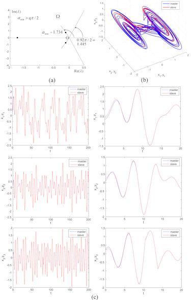
: q1=q2=q3=0.92subscript𝑞1subscript𝑞2subscript𝑞30.92q_{1}=q_{2}=q_{3}=0.92. The eigenvalues of E𝐸E are λ1=1.755subscript𝜆11.755\lambda_{1}=-1.755 and λ2,3=0.123±0.745isubscript𝜆23plus-or-minus0.1230.745𝑖\lambda_{2,3}=-0.123\pm 0.745i with arguments arg(λ1)=π𝑎𝑟𝑔subscript𝜆1𝜋arg(\lambda_{1})=\pi (λ1subscript𝜆1\lambda_{1} is located on the negative real axis where a complex number has arg=π𝑎𝑟𝑔𝜋arg=\pi), and arg(λ2,3)=±1.734𝑎𝑟𝑔subscript𝜆23plus-or-minus1.734arg(\lambda_{2,3})=\pm 1.734. Therefore αmin=1.734>1.445=0.92π/2subscript𝛼𝑚𝑖𝑛1.7341.4450.92𝜋2\alpha_{min}=1.734>1.445=0.92\pi/2 and all eigenvalues are located inside the asymptotically stability region ΩΩ\Omega (Fig. 8a) and the systems synchronize (see Fig. 8b and Fig. 8c).

Remark 4.

Generally, the controller u𝑢u for systems defined as Dqxi=xi+1subscriptsuperscript𝐷𝑞subscript𝑥𝑖subscript𝑥𝑖1D^{q}_{*}x_{i}=x_{i+1}, i=1,2,,n1𝑖12𝑛1i=1,2,...,n-1, and Dqxn=f(x)superscriptsubscript𝐷𝑞subscript𝑥𝑛𝑓𝑥D_{*}^{q}x_{n}=f(x), can be defined for only the n𝑛nth equation.

Incommensurate case

: q=(0.9,1,0.9)𝑞0.910.9q=(0.9,1,0.9). Let us consider the master-slave system (27)-(28) with the same controller. m=10𝑚10m=10, and the characteristic polynomial (19) is

P(λ):=λ28+2λ19+λ9+1.assign𝑃𝜆superscript𝜆282superscript𝜆19superscript𝜆91P(\lambda):=\lambda^{28}+2\lambda^{19}+\lambda^{9}+1. (31)

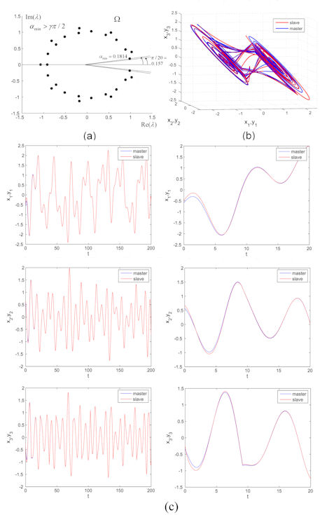
The images of the 282828 complex roots are situated inside the stability region ΩΩ\Omega and αmin=0.1814>0.1571=π/20subscript𝛼𝑚𝑖𝑛0.18140.1571𝜋20\alpha_{min}=0.1814>0.1571=\pi/20 (Fig. 9a) and the two systems synchronize (Fig. 9b and Fig. 9c).

4.2 Chen system

Let the master system

Dq1x1=a(x2x1),Dq2x2=(cax3)sgn~(x1)+cdx2,Dq3x3=x1sgn~(x2)bx3,superscriptsubscript𝐷subscript𝑞1subscript𝑥1𝑎subscript𝑥2subscript𝑥1superscriptsubscript𝐷subscript𝑞2subscript𝑥2𝑐𝑎subscript𝑥3~𝑠𝑔𝑛subscript𝑥1𝑐𝑑subscript𝑥2superscriptsubscript𝐷subscript𝑞3subscript𝑥3subscript𝑥1~𝑠𝑔𝑛subscript𝑥2𝑏subscript𝑥3\begin{array}[]{l}D_{\ast}^{q_{1}}x_{1}=a\left(x_{2}-x_{1}\right),\\ D_{\ast}^{q_{2}}x_{2}=\left(c-a-x_{3}\right)\widetilde{sgn}(x_{1})+cdx_{2},\\ D_{\ast}^{q_{3}}x_{3}=x_{1}\widetilde{sgn}(x_{2})-bx_{3},\end{array} (32)

and the slave system

Dq1y1=a(y2y1)+u1,Dq2y2=(cay3)sgn~(y1)+cdy2+u2,Dq3y3=y1sgn~(y2)by3+u3.superscriptsubscript𝐷subscript𝑞1subscript𝑦1𝑎subscript𝑦2subscript𝑦1subscript𝑢1superscriptsubscript𝐷subscript𝑞2subscript𝑦2𝑐𝑎subscript𝑦3~𝑠𝑔𝑛subscript𝑦1𝑐𝑑subscript𝑦2subscript𝑢2superscriptsubscript𝐷subscript𝑞3subscript𝑦3subscript𝑦1~𝑠𝑔𝑛subscript𝑦2𝑏subscript𝑦3subscript𝑢3\begin{array}[]{l}D_{\ast}^{q_{1}}y_{1}=a\left(y_{2}-y_{1}\right)+u_{1},\\ D_{\ast}^{q_{2}}y_{2}=\left(c-a-y_{3}\right)\widetilde{sgn}(y_{1})+cdy_{2}+u_{2},\\ D_{\ast}^{q_{3}}y_{3}=y_{1}\widetilde{sgn}(y_{2})-by_{3}+u_{3}.\end{array} (33)

With the initial conditions x(0)=[0.009,0.012,0.020]T𝑥0superscript0.0090.0120.020𝑇x(0)=[-0.009,-0.012,\allowbreak 0.020]^{T} and y(0)=x(0)+[0.005,0.005,0.005]T𝑦0𝑥0superscript0.0050.0050.005𝑇y(0)=x(0)+[0.005,0.005,0.005]^{T}444The relatively small difference between x(0)𝑥0x(0) and y(0)𝑦0y(0) is in agreement with the small size of attractor, which as can be see in, e.g., Fig. 11, is of order of 102superscript10210^{-2}, and also avoid long transients before the trajectories reach the attractors., if we chose the controller u=(u1,u2,u3)T𝑢superscriptsubscript𝑢1subscript𝑢2subscript𝑢3𝑇u=(u_{1},u_{2},u_{3})^{T}

u1=ae2+(a2)e1,u2=(cax3)sgn~(x1)(cay3)sgn~(y1)(cd+1)e2,u3=x1sgn~(x2)y1sgn~(y2)+(b3)e3,subscript𝑢1absent𝑎subscript𝑒2𝑎2subscript𝑒1subscript𝑢2absent𝑐𝑎subscript𝑥3~𝑠𝑔𝑛subscript𝑥1𝑐𝑎subscript𝑦3~𝑠𝑔𝑛subscript𝑦1missing-subexpression𝑐𝑑1subscript𝑒2subscript𝑢3absentsubscript𝑥1~𝑠𝑔𝑛subscript𝑥2subscript𝑦1~𝑠𝑔𝑛subscript𝑦2𝑏3subscript𝑒3\begin{array}[]{ll}u_{1}&=-ae_{2}+(a-2)e_{1},\\ u_{2}&=(c-a-x_{3})\widetilde{sgn}(x_{1})-(c-a-y_{3})\widetilde{sgn}(y_{1})\\ &-(cd+1)e_{2},\\ u_{3}&=x_{1}\widetilde{sgn}(x_{2})-y_{1}\widetilde{sgn}(y_{2})+(b-3)e_{3},\end{array}

where ei=yixisubscript𝑒𝑖subscript𝑦𝑖subscript𝑥𝑖e_{i}=y_{i}-x_{i}, i=1,2,3𝑖123i=1,2,3, the following error system is obtained

Dq1e1=2e1,Dq2e2=e2,Dq3e3=3e3.superscriptsubscript𝐷subscript𝑞1subscript𝑒12subscript𝑒1superscriptsubscript𝐷subscript𝑞2subscript𝑒2subscript𝑒2superscriptsubscript𝐷subscript𝑞3subscript𝑒33subscript𝑒3\begin{array}[]{l}D_{\ast}^{q_{1}}e_{1}=-2e_{1},\\ D_{\ast}^{q_{2}}e_{2}=-e_{2},\\ D_{\ast}^{q_{3}}e_{3}=-3e_{3}.\end{array} (34)

Here E𝐸E

E=(200010003).𝐸200010003E=\left(\begin{array}[]{ccc}-2&0&0\\ 0&-1&0\\ 0&0&-3\end{array}\right).

Commensurate case

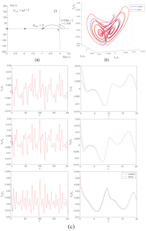
: q1=q2=q3=0.998subscript𝑞1subscript𝑞2subscript𝑞30.998q_{1}=q_{2}=q_{3}=0.998. The eigenvalues of the Jacobian matrix are Λ=(3,2,1)Λ321\Lambda=(-3,-2,-1) with αmin=π>1.568=0.998π/2subscript𝛼𝑚𝑖𝑛𝜋1.5680.998𝜋2\alpha_{min}=\pi>1.568=0.998\pi/2 (Fig. 10a) and the synchronization can be made since the eigenvalues belong to ΩΩ\Omega (Fig. 10b and Fig. 10c).

Incommensurate case

: q=(0.99,0.98,0.97)𝑞0.990.980.97q=(0.99,0.98,0.97). The fractional error system is asymptotically stable because, the roots of the underlying characteristic equation (19)

(λ99+2)(λ98+1)(λ97+3)=0,superscript𝜆992superscript𝜆981superscript𝜆9730(\lambda^{99}+2)(\lambda^{98}+1)(\lambda^{97}+3)=0,

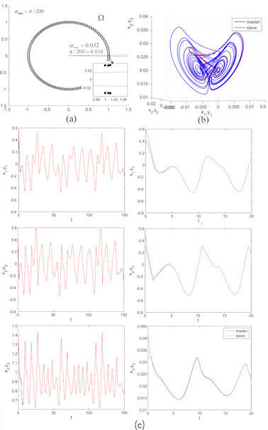
are placed in ΩΩ\Omega (Fig. 11a) and αmin=0.032>0.016=π/200subscript𝛼𝑚𝑖𝑛0.0320.016𝜋200\alpha_{min}=0.032>0.016=\pi/200. The two systems synchronize (Fig. 11b and 11c).

4.3 Shimizu–Morioka system

The fractional variant of the piece-wise continuous Shimizu Morioka’s system has the following mathematical model [19, 20]

Dq1x1=x2,Dq2x2=sgn~(x1)x3sgn~(x1)αx2,Dq3x3=x12βx3,superscriptsubscript𝐷subscript𝑞1subscript𝑥1subscript𝑥2superscriptsubscript𝐷subscript𝑞2subscript𝑥2~𝑠𝑔𝑛subscript𝑥1subscript𝑥3~𝑠𝑔𝑛subscript𝑥1𝛼subscript𝑥2superscriptsubscript𝐷subscript𝑞3subscript𝑥3superscriptsubscript𝑥12𝛽subscript𝑥3\begin{array}[]{l}D_{\ast}^{q_{1}}x_{1}=x_{2},\\ D_{\ast}^{q_{2}}x_{2}=\widetilde{sgn}(x_{1})-x_{3}\widetilde{sgn}(x_{1})-\alpha x_{2},\\ D_{\ast}^{q_{3}}x_{3}=x_{1}^{2}-\beta x_{3},\end{array} (35)

where α=0.75𝛼0.75\alpha=0.75 and β=0.45𝛽0.45\beta=0.45. Beside the origin, the other two equilibrium points are X~1,2=(±β,0,1)subscriptsuperscript~𝑋12plus-or-minus𝛽01\tilde{X}^{*}_{1,2}=(\pm\sqrt{\beta},0,1) and the Jacobian is

J~=(0100αsgn(x1)2x10β)X~1,2.~𝐽subscript0100𝛼𝑠𝑔𝑛subscript𝑥12subscript𝑥10𝛽subscriptsuperscript~𝑋12\tilde{J}=\left(\begin{array}[]{ccc}0&1&0\\ 0&-\alpha&-sgn(x_{1})\\ 2x_{1}&0&-\beta\end{array}\right)_{\tilde{X}^{\ast}_{1,2}}.

Again Properties 3 and 3 have been used.

Let (35) be the master system and

Dq1y1=y2+u1,Dq2y2=sgn~(y1)y3sgn~(y1)αy2+u2,Dq3y3=y12βy3+u3.superscriptsubscript𝐷subscript𝑞1subscript𝑦1subscript𝑦2subscript𝑢1superscriptsubscript𝐷subscript𝑞2subscript𝑦2~𝑠𝑔𝑛subscript𝑦1subscript𝑦3~𝑠𝑔𝑛subscript𝑦1𝛼subscript𝑦2subscript𝑢2superscriptsubscript𝐷subscript𝑞3subscript𝑦3superscriptsubscript𝑦12𝛽subscript𝑦3subscript𝑢3\begin{array}[]{l}D_{\ast}^{q_{1}}y_{1}=y_{2}+u_{1},\\ D_{\ast}^{q_{2}}y_{2}=\widetilde{sgn}(y_{1})-y_{3}\widetilde{sgn}(y_{1})-\alpha y_{2}+u_{2},\\ D_{\ast}^{q_{3}}y_{3}=y_{1}^{2}-\beta y_{3}+u_{3}.\end{array} (36)

the slave system.

If we chosen u1=e1e2subscript𝑢1subscript𝑒1subscript𝑒2u_{1}=-e_{1}-e_{2}, u2=sgn~(y1)+y3sgn~(y1)+sgn~(x1)x3sgn~(x1)subscript𝑢2~𝑠𝑔𝑛subscript𝑦1subscript𝑦3~𝑠𝑔𝑛subscript𝑦1~𝑠𝑔𝑛subscript𝑥1subscript𝑥3~𝑠𝑔𝑛subscript𝑥1u_{2}=-\widetilde{sgn}(y_{1})+y_{3}\widetilde{sgn}(y_{1})+\widetilde{sgn}(x_{1})-x_{3}\widetilde{sgn}(x_{1}) and u3=y12+x12subscript𝑢3superscriptsubscript𝑦12superscriptsubscript𝑥12u_{3}=-y_{1}^{2}+x_{1}^{2}, the error system is

Dq1e1=e1,Dq2e2=αe2,Dq3e3=βe3.superscriptsubscript𝐷subscript𝑞1subscript𝑒1subscript𝑒1superscriptsubscript𝐷subscript𝑞2subscript𝑒2𝛼subscript𝑒2superscriptsubscript𝐷subscript𝑞3subscript𝑒3𝛽subscript𝑒3\begin{array}[]{l}D_{\ast}^{q_{1}}e_{1}=-e_{1},\\ D_{\ast}^{q_{2}}e_{2}=-\alpha e_{2},\\ D_{\ast}^{q_{3}}e_{3}=-\beta e_{3}.\end{array} (37)

Let next consider X~1superscriptsubscript~𝑋1\tilde{X}_{1}^{*}.

Commensurate case

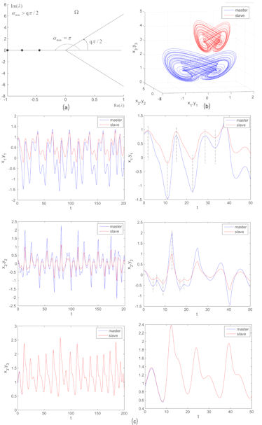
: q1=q2=q3=0.9subscript𝑞1subscript𝑞2subscript𝑞30.9q_{1}=q_{2}=q_{3}=0.9. Then Λ=(1.000,0.750,0.450)Λ1.0000.7500.450\Lambda=(-1.000,-0.750,-0.450) and αmin=π>1.445=0.9π/2subscript𝛼𝑚𝑖𝑛𝜋1.4450.9𝜋2\alpha_{min}=\pi>1.445=0.9\pi/2 (Fig. 12a). Therefore the systems synchronize (Fig. 12b and Fig. 12c).

Incommensurate case

: q=(0.9,1,0.9)𝑞0.910.9q=(0.9,1,0.9). Then the characteristic polynomial is

λ28+9/20λ19+3/4λ18+27/80λ9+3/55,superscript𝜆28920superscript𝜆1934superscript𝜆182780superscript𝜆9355\lambda^{28}+9/20\lambda^{19}+3/4\lambda^{18}+27/80\lambda^{9}+3/5\sqrt{5},

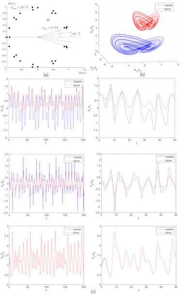
and ΛΛ\Lambda containing the 28 roots is included in the stability region ΩΩ\Omega (Fig. 13a). αmin=0.314>0.157=π/20subscript𝛼𝑚𝑖𝑛0.3140.157𝜋20\alpha_{min}=0.314>0.157=\pi/20 and therefore the systems synchronize (Fig. 13b and Fig. 13c).

Remark 5.

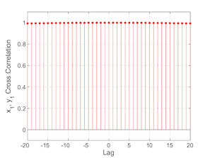
As can be seen in Fig. 12 and Fig. 13, for this system, the synchronization is of phase synchronization-like type (see e.g. [21]): occurrence of a certain relation between the phases of interacting systems, while the amplitudes remain chaotic and are, in general, uncorrelated. In Fig. 14 the value +11+1 of the cross correlation determined for the components x1subscript𝑥1x_{1} and y1subscript𝑦1y_{1}, underlines the perfect phase synchronization. Similar result is obtained for x2subscript𝑥2x_{2} and y2subscript𝑦2y_{2}. This phenomenon happens only with respect to x1,2subscript𝑥12x_{1,2} and y1,2subscript𝑦12y_{1,2}, while along x3subscript𝑥3x_{3} axis the synchronization is a complete (identical) synchronization.

4.4 Chen-Sprott systems

Finally, let consider the synchronization of two non-identical systems: a Chen system and a Sprott system.

Let us consider Sprott’s system (27) the master system and Chen’s system (33) the slave system.

With u1=a(y2y1)+x23e1subscript𝑢1𝑎subscript𝑦2subscript𝑦1subscript𝑥23subscript𝑒1u_{1}=-a(y_{2}-y_{1})+x_{2}-3e_{1}, u2=(cay3)sgn~(y1)cdy2+x32e2subscript𝑢2𝑐𝑎subscript𝑦3~𝑠𝑔𝑛subscript𝑦1𝑐𝑑subscript𝑦2subscript𝑥32subscript𝑒2u_{2}=-(c-a-y_{3})\widetilde{sgn}(y_{1})-cdy_{2}+x_{3}-2e_{2} and u3=y1sgn~(y2)+by3x1x20.5y3+sgn~(x1)e3subscript𝑢3subscript𝑦1~𝑠𝑔𝑛subscript𝑦2𝑏subscript𝑦3subscript𝑥1subscript𝑥20.5subscript𝑦3~𝑠𝑔𝑛subscript𝑥1subscript𝑒3u_{3}=-y_{1}\widetilde{sgn}(y_{2})+by_{3}-x_{1}-x_{2}-0.5y_{3}+\widetilde{sgn}(x_{1})-e_{3}, one obtains the following error system

Dq1e1=3e1,Dq2e2=2e2,Dq3e3=e3,superscriptsubscript𝐷subscript𝑞1subscript𝑒13subscript𝑒1superscriptsubscript𝐷subscript𝑞2subscript𝑒22subscript𝑒2superscriptsubscript𝐷subscript𝑞3subscript𝑒3subscript𝑒3\begin{array}[]{l}D_{\ast}^{q_{1}}e_{1}=-3e_{1},\\ D_{\ast}^{q_{2}}e_{2}=-2e_{2},\\ D_{\ast}^{q_{3}}e_{3}=-e_{3},\end{array} (38)

with the error matrix

E=(300020001).𝐸300020001E=\left(\begin{array}[]{ccc}-3&0&0\\ 0&-2&0\\ 0&0&-1\end{array}\right).

Commensurate case

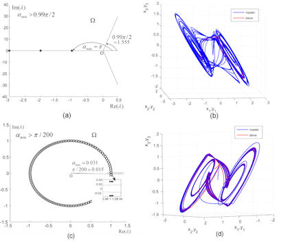
: q1=q2=q3=0.99subscript𝑞1subscript𝑞2subscript𝑞30.99q_{1}=q_{2}=q_{3}=0.99. The eigenvalues are (3,2,1)321(-3,-2,-1) and αmin=π>1.555=0.99π/2subscript𝛼𝑚𝑖𝑛𝜋1.5550.99𝜋2\alpha_{min}=\pi>1.555=0.99\pi/2 (Fig. 15a). Therefore the error sysem is asymptotically stable and the two systems synchronize (Fig. 15b).

Incommensurate case

: q=(0.99,0.98,0.97)𝑞0.990.980.97q=(0.99,0.98,0.97). The characteristic equation is

(λ99+3)(λ98+2)(λ97+1)=0,superscript𝜆993superscript𝜆982superscript𝜆9710(\lambda^{99}+3)(\lambda^{98}+2)(\lambda^{97}+1)=0,

for which αmin=0.031>0.015=π/200subscript𝛼𝑚𝑖𝑛0.0310.015𝜋200\alpha_{min}=0.031>0.015=\pi/200. Therefore ΛΩΛΩ\Lambda\subset\Omega (Fig. 15c) and the systems synchronize, Chen’s system following the master system, Sprott’s system (Fig. 15d).

5 Conclusion and discussions

In this paper we presented a way to synchronize a class of piece-wise systems of fractional-order. This is achievable due to the possibility to approximate continuously the piece-wise functions modeling the underlying systems. The approximation is realized via Cellina’s Theorem for set-valued functions, after the piece-wise functions s𝑠s have been transformed into set-valued functions with the Filippov’s regularization. There are several approximation choices. In this paper we use the sigmoid function, which is easy to implement numerically.

Once the systems approximated, the synchronization problem transforms into a synchronization of two (identical or not) continuous systems of fractional-order.

The known stability results for continuous systems of fractional-order, have been adapted for our class of problems.

The sigmoid function used in this paper can be replaced with other continuous approximation.

The approximation algorithm can be used for other purpose too, such as chaos control.

Appendix

A. Cellina’s Theorem

Theorem 1 (Cellina’s Theorem [2] p. 84 and [3] p. 358).

Let F:nn:𝐹superscript𝑛superscript𝑛F:\mathbb{R}^{n}\rightrightarrows\mathbb{R}^{n} be an u.s.c. function. If the values of F𝐹F are nonempty and convex, then for every ε>0𝜀0\varepsilon>0, there exists a locally Lipschitz single values function fε:nn:subscript𝑓𝜀superscript𝑛superscript𝑛f_{\varepsilon}:\mathbb{R}^{n}\rightarrow\mathbb{R}^{n} such that

Graph(fε)B(Graph(F),ε),𝐺𝑟𝑎𝑝subscript𝑓𝜀𝐵𝐺𝑟𝑎𝑝𝐹𝜀Graph(f_{\varepsilon})\subset B(Graph(F),\varepsilon), (A.1)

and for every xn𝑥superscript𝑛x\in\mathbb{R}^{n}, fε(x)subscript𝑓𝜀𝑥f_{\varepsilon}(x) belongs to teh convex hull of the image of F𝐹F.

In (A.1), B𝐵B is the ball in nsuperscript𝑛\mathbb{R}^{n} centered on F𝐹F and of ε𝜀\varepsilon ray.

See for example Fig. 1b.

As known, locally Lipschitz functions are also continuous.

B. Proof of Property 1

We shall prove that, for every δ>0𝛿0\delta>0, there exists ε>0𝜀0\varepsilon>0 such that |sgn~(x)1|<ε~𝑠𝑔𝑛𝑥1𝜀|\widetilde{sgn}(x)-1|<\varepsilon. Solving the inequality, one obtains: x(,δln2εε)(δlnε2ε,)𝑥𝛿𝑙𝑛2𝜀𝜀𝛿𝑙𝑛𝜀2𝜀x\in(-\infty,-\delta ln\frac{2-\varepsilon}{\varepsilon})\bigcup(-\delta ln\frac{\varepsilon}{2-\varepsilon},\infty). For ε0𝜀0\varepsilon\rightarrow 0, δln2εε𝛿𝑙𝑛2𝜀𝜀-\delta ln\frac{2-\varepsilon}{\varepsilon} and δlnε2ε𝛿𝑙𝑛𝜀2𝜀-\delta ln\frac{\varepsilon}{2-\varepsilon} tend to 0. Therefore sgn~(x)Sgn(x)~𝑠𝑔𝑛𝑥𝑆𝑔𝑛𝑥\widetilde{sgn}(x)\approx Sgn(x) for x𝒱=(δln2εε,δlnε2ε)𝑥𝒱𝛿𝑙𝑛2𝜀𝜀𝛿𝑙𝑛𝜀2𝜀x\not\in\mathcal{V}=(-\delta ln\frac{2-\varepsilon}{\varepsilon},-\delta ln\frac{\varepsilon}{2-\varepsilon}) and, consequently, X~Xsuperscript~𝑋superscript𝑋\tilde{X}^{*}\approx X^{*}. ∎

For ε{0,2}𝜀02\varepsilon\in\{0,2\}, ln𝑙𝑛ln is not defined. However, our interest concerns ε2,0𝜀20\varepsilon\neq 2,0.

C. Proof of Property 2

We prove that for every δ>0𝛿0\delta>0 there exists ε>0𝜀0\varepsilon>0 such that |ddxsgn~(x)|<ε𝑑𝑑𝑥~𝑠𝑔𝑛𝑥𝜀|\frac{d}{dx}\widetilde{sgn}(x)|<\varepsilon. By solving the inequality ddxsgn~(x)=2ex/dδ(ex/d+1)2<ε𝑑𝑑𝑥~𝑠𝑔𝑛𝑥2superscript𝑒𝑥𝑑𝛿superscriptsuperscript𝑒𝑥𝑑12𝜀\frac{d}{dx}\widetilde{sgn}(x)=\frac{2e^{x/d}}{\delta(e^{x/d}+1)^{2}}<\varepsilon (Fig. 5a), one obtains |x|>δln12δε+δε1δε𝑥𝛿𝑙𝑛12𝛿𝜀𝛿𝜀1𝛿𝜀|x|>\delta ln\frac{\sqrt{1-2\delta\varepsilon}+\delta\varepsilon-1}{\delta\varepsilon} (Fig. 5b). On the other side, for x0𝑥0x\neq 0, ddxsgn(x)=0𝑑𝑑𝑥𝑠𝑔𝑛𝑥0\frac{d}{dx}sgn(x)=0. Therefore, for x𝒱=(δln12δε+δε1δε,δln12δε+δε1δε)𝑥𝒱𝛿𝑙𝑛12𝛿𝜀𝛿𝜀1𝛿𝜀𝛿𝑙𝑛12𝛿𝜀𝛿𝜀1𝛿𝜀x\not\in\mathcal{V}=(-\delta ln\frac{\sqrt{1-2\delta\varepsilon}+\delta\varepsilon-1}{\delta\varepsilon},\delta ln\frac{\sqrt{1-2\delta\varepsilon}+\delta\varepsilon-1}{\delta\varepsilon}), ddxsgn~(x)ddxsgn(x)𝑑𝑑𝑥~𝑠𝑔𝑛𝑥𝑑𝑑𝑥𝑠𝑔𝑛𝑥\frac{d}{dx}\widetilde{sgn}(x)\approx\frac{d}{dx}sgn(x) and therefore J~J~𝐽𝐽\tilde{J}\approx J for x𝒱𝑥𝒱x\not\in\mathcal{V}. ∎

Above, beside Assumption (H2), it is supposed that xisgn(xj)subscript𝑥𝑖𝑠𝑔𝑛subscript𝑥𝑗x_{i}sgn(x_{j}), for i,j1,2,,nformulae-sequence𝑖𝑗12𝑛i,j\in{1,2,...,n}, is differentiable on the interior of 𝒟isubscript𝒟𝑖\mathcal{D}_{i}.

D. Hausdorff distance

The Hausdorff distance (or Hausdorff metric) DHsubscript𝐷𝐻D_{H} measures how far two compact nonempty subsets of the considered metric space nsuperscript𝑛\mathbb{R}^{n} are from each other [22]. The Hausdorff distance between two curves in (here nsuperscript𝑛\mathbb{R}^{n}) is defined as the maximum distance to the closest point between the curves. If the curves are defined, as in our case, as the sets of ordered pair of coordinates A={P1,P2,,Pm1}𝐴subscript𝑃1subscript𝑃2subscript𝑃subscript𝑚1A=\{P_{1},P_{2},...,P_{m_{1}}\} and B={Q1,Q2,,Qm2}𝐵subscript𝑄1subscript𝑄2subscript𝑄subscript𝑚2B=\{Q_{1},Q_{2},...,Q_{m_{2}}\} with Pi=(x1,x2,,xn)subscript𝑃𝑖subscript𝑥1subscript𝑥2subscript𝑥𝑛P_{i}=(x_{1},x_{2},...,x_{n}) and Qi={y1,y2,,yn)subscript𝑄𝑖subscript𝑦1subscript𝑦2subscript𝑦𝑛Q_{i}=\{y_{1},y_{2},...,y_{n}), then DHsubscript𝐷𝐻D_{H} is expressed as follows

DH(P,Q)=max{d(P,Q),d(Q,P)},subscript𝐷𝐻𝑃𝑄𝑚𝑎𝑥𝑑𝑃𝑄𝑑𝑄𝑃D_{H}(P,Q)=max\{d(P,Q),d(Q,P)\},

where d(P,Q)𝑑𝑃𝑄d(P,Q) (generally differen to d(Q,P)𝑑𝑄𝑃d(Q,P)) has the expression

d(P,Q)=max𝑖{d(Pi,Q)},𝑑𝑃𝑄𝑖𝑚𝑎𝑥𝑑subscript𝑃𝑖𝑄d(P,Q)=\underset{i}{max}\{d(P_{i},Q)\},

and

d(Pi,Q)=max𝑗PiQj.𝑑subscript𝑃𝑖𝑄𝑗𝑚𝑎𝑥normsubscript𝑃𝑖subscript𝑄𝑗d(P_{i},Q)=\underset{j}{max}||P_{i}-Q_{j}||.

References

  • [1] Filippov, A.F. Differential Equations with Discontinuous Right-Hand Sides. Kluwer Academic, Dordrecht (1988)
  • [2] Aubin, J.-P., Cellina, A. Differential Inclusions Set-valued Maps and Viability Theory. Springer, Berlin (1984)
  • [3] Aubin, J.-P., Frankowska, H. Set-valued Analysis. Birkh user, Boston (1990)
  • [4] Diethlem, K., Ford, N., Freed, A. D. Predictor-Corrector Approach for the Numerical Solution of Fractional Differential Equations. Nonlinear Dyn. 29, 3–22 (2002)
  • [5] Diethelm, K., Ford, N.J. Analysis of fractional differential equations. J. Math. Anal. Appl. 265, 229 -248 (2002)
  • [6] Dontchev, A., Lempio, F. Difference methods for differen- tial inclusions. SIAM Rev. 34, 263- 294 (1992)
  • [7] Kastner-Maresch, A., Lempio, F. Difference methods with selection strategies for differential inclusions. Numer. Funct. Anal. Optim. 14, 555 -572 (1993)
  • [8] Oldham, K.B., Spanier, J. The Fractional Calculus: The- ory and Applications of Differentiation and Integration of Arbitrary Order. Academic Press, New York (1974)
  • [9] Caputo, M.: Linear models of dissipation whose Q is al- most frequency independent–II. Geophys. J. R. Astron. Soc. 13, 529 539 (1967); reprinted in Fract. Calc. Appl. Anal. 10(3), 309 324 (2007)
  • [10] Podlubny, I. Fractional Differential Equations. Academic Press, San Diego (1999)
  • [11] Aziz-Alaoui, M.A., Chen, G. Asymptotic analysisof a new piecewise-linearchaotic system. Int. J. Bifurc. Chaos 12(1), 147 -157 (2002)
  • [12] Danca, M.-F. Continuous approximations of a class of piece-wise continuous systems, submitted.
  • [13] Matignon, D. Stability properties for generalized fractional differential systems. ESAIM: Proc. 5, 145 -158 (1998)
  • [14] Deng, W., Li, C., L , J. Stability analysis of linear fractional differential system with multiple time delays. Nonlinear Dyn. 48, 409 -416 (2007)
  • [15] Tavazoei, M. S., Haeri, M. Limitations of frequency domain approximation for detecting chaos in fractional order systems. Nonlinear Analysis 69, 1299 -1320 (2008).
  • [16] Tavazoei, M. S., Haeri, M. Chaotic attractors in incommensurate fractional order systems. Physica D 237, 2628–2637 (2008)
  • [17] Sprott, J.C. A new class of chaotic circuit. Phys. Lett. A 266, 19 -23 (2000)
  • [18] Ahmad, W.M., Sprott, J.C. Chaos in fractional-order autonomous nonlinear systems. Chaos Solitons & Fractals 16, 339 -351 (2003)
  • [19] Shimizu T., Morioka, N. On the bifurcation of a symmetric limit cycle to an asymmetric one in a simple model. Phys. Lett. A, 76, 201- 204 (1980)
  • [20] Yu, S., Tang, W.K.S., Lü, J., Chen, G. Generation of n×m𝑛𝑚n\times m-Wing Lorenz-Like Attractors From a Modified Shimizu–Morioka Model. Circuits and Systems II: Express Briefs, IEEE Transactions on, 55 (11), 1168–1172 (2008)
  • [21] Rosenblum, M.G., Pikovsky, A.S., Kurths, J. Phase Synchronization of Chaotic Oscillators. Phys. Rev. Lett. 76, 1804 (1996)
  • [22] Falconer, K.: Fractal Geometry, Mathematical Foundations and Applications. John Wiley and Sons, Chichester (1990)
Refer to caption
Figure 1: a) Graph of f(x)=23sgn(x)𝑓𝑥23𝑠𝑔𝑛𝑥f(x)=2-3sgn(x). b) Graph of set-valued function F(x)=23Sgn(x)𝐹𝑥23𝑆𝑔𝑛𝑥F(x)=2-3Sgn(x) (blue) and continuous approximation of F(x)𝐹𝑥F(x) (red).
Refer to caption
Figure 2: a) Graph of sgn𝑠𝑔𝑛sgn function. b) Graph of Sgn𝑆𝑔𝑛Sgn function.
Refer to caption
Figure 3: Graph of sigmoid function sgn~~𝑠𝑔𝑛\widetilde{sgn}. a) Dependence on δ𝛿\delta. b) Graph of sgn~~𝑠𝑔𝑛\widetilde{sgn} for several values δ𝛿\delta.
Refer to caption
Figure 4: Continuous approximation algorithm. Dotted line shows the direct way to approximate the discontinuous components s𝑠s.
Refer to caption
Figure 5: a) Graph of ddxsgn~𝑑𝑑𝑥~𝑠𝑔𝑛\frac{d}{dx}\widetilde{sgn}, function on δ𝛿\delta. ΔΔ\Delta and ε𝜀\varepsilon represent vertical and horizontal planes through some δ𝛿\delta and ε𝜀\varepsilon values. b) Graph of ddxsgn~𝑑𝑑𝑥~𝑠𝑔𝑛\frac{d}{dx}\widetilde{sgn} for δ=1/10𝛿110\delta=1/10 and ε=0.2𝜀0.2\varepsilon=0.2 (δ𝛿\delta and ε𝜀\varepsilon have been chosen larger for a clearer image).
Refer to caption
Figure 6: a) Stability domain ΩΩ\Omega determined by αmin>γπ/2subscript𝛼𝑚𝑖𝑛𝛾𝜋2\alpha_{min}>\gamma\pi/2. b) Instability domain ΦΦ\Phi determined by αminγπ/2subscript𝛼𝑚𝑖𝑛𝛾𝜋2\alpha_{min}\leq\gamma\pi/2. d1,2subscript𝑑12d_{1,2} are the stability separatrices.
Refer to caption
Figure 7: Chaotic Piece-wise linear Chen system for: top q=0.99𝑞0.99q=0.99; bottom q=(1,0.9,1)𝑞10.91q=(1,0.9,1). a) Commensurate case q=0.99𝑞0.99q=0.99, αmin<0.99π/2subscript𝛼𝑚𝑖𝑛0.99𝜋2\alpha_{min}<0.99\pi/2 and the system is unstable. b) The underlying chaotic attractor. c) Incommensurate q=(1,0.9,1)𝑞10.91q=(1,0.9,1), αmin<π/20subscript𝛼𝑚𝑖𝑛𝜋20\alpha_{min}<\pi/20 and the system is unstable. d) The underlying chaotic attractor.
Refer to caption
Figure 8: Synchronization of Sprott system for q=0.92𝑞0.92q=0.92. a) αmin>0.92π/2subscript𝛼𝑚𝑖𝑛0.92𝜋2\alpha_{min}>0.92\pi/2 and the error system is stable and synchronization holds. b) Phase plot of both trajectories (in blue the master system, in red the slave system). c) Time series: left column t[0,200]𝑡0200t\in[0,200], right column t[0,20]𝑡020t\in[0,20].
Refer to caption
Figure 9: Synchronization of Sprott system for q=(0.9,1,0.9)𝑞0.910.9q=(0.9,1,0.9). a) αmin>π/20subscript𝛼𝑚𝑖𝑛𝜋20\alpha_{min}>\pi/20 and the error system is stable and synchronization holds. b) Phase plot of both trajectories (in blue the master system, in red the slave system). c) Time series: left column t[0,200]𝑡0200t\in[0,200], right column t[0,20]𝑡020t\in[0,20].
Refer to caption
Figure 10: Synchronization of piece-wise Chen system for q1=q2=q3=0.998subscript𝑞1subscript𝑞2subscript𝑞30.998q_{1}=q_{2}=q_{3}=0.998. a) αmin>0.998π/2subscript𝛼𝑚𝑖𝑛0.998𝜋2\alpha_{min}>0.998\pi/2 and the error system is stable and synchronization holds. b) Phase plot of both trajectories (in blue the master system, in red the slave system). c) Time series: left column t[0,200]𝑡0200t\in[0,200], right column t[0,20]𝑡020t\in[0,20].
Refer to caption
Figure 11: Synchronization of piece-wise Chen system for q=(0.99,0.98,0.97)𝑞0.990.980.97q=(0.99,0.98,0.97). a) αmin>π/200subscript𝛼𝑚𝑖𝑛𝜋200\alpha_{min}>\pi/200 and the error system is stable and synchronization holds. Detail reveal the positions of the roots versus the separatrices. b)Phase plot of both trajectories (in blue the master system, in red the slave system). c) Time series: left column t[0,200]𝑡0200t\in[0,200], right column t[0,20]𝑡020t\in[0,20].
Refer to caption
Figure 12: Synchronization of piece-wise Shimizu- Morioka system for q1=q2=q3=0.9subscript𝑞1subscript𝑞2subscript𝑞30.9q_{1}=q_{2}=q_{3}=0.9. a) αmin=π>0.9π/2subscript𝛼𝑚𝑖𝑛𝜋0.9𝜋2\alpha_{min}=\pi>0.9\pi/2 and the error system is stable and synchronization holds. b)Phase plot of both trajectories (in blue the master system, in red the slave system). c) Time series: left column t[0,200]𝑡0200t\in[0,200], right column t[0,20]𝑡020t\in[0,20]. Dotted lines underline phase synchronization.
Refer to caption
Figure 13: Synchronization of piece-wise Shimizu -Morioka system for q=(0.9,1,0.9)𝑞0.910.9q=(0.9,1,0.9). a) αmin=0.314>π/20subscript𝛼𝑚𝑖𝑛0.314𝜋20\alpha_{min}=0.314>\pi/20 and the error system is stable and synchronization holds. b) Plot of both trajectories translated along x3subscript𝑥3x_{3} axis (in blue the master system, in red the slave system). c) Time series: left column t[0,200]𝑡0200t\in[0,200], right column t[0,20]𝑡020t\in[0,20]. Dotted lines underline phase synchronization.
Refer to caption
Figure 14: Cross correlation for the components x1subscript𝑥1x_{1} and y1subscript𝑦1y_{1} of two Shimizu -Morioka synchronized systems. x1subscript𝑥1x_{1} and y1subscript𝑦1y_{1} are in phase since the value of the cross correlation is +11+1.
Refer to caption
Figure 15: Synchronization of Sprott’s system and piece-wise Chen’s system. a) For q1=q2=q3=0.99subscript𝑞1subscript𝑞2subscript𝑞30.99q_{1}=q_{2}=q_{3}=0.99, αmin>0.99π/2subscript𝛼𝑚𝑖𝑛0.99𝜋2\alpha_{min}>0.99\pi/2 and the error system is stable and synchronization holds. b) Phase plot of both trajectories translated along x3subscript𝑥3x_{3} axis (in blue the master system, in red the slave system). c) For q=(0.99,098,0.97)𝑞0.990980.97q=(0.99,098,0.97), αmin>π/200subscript𝛼𝑚𝑖𝑛𝜋200\alpha_{min}>\pi/200 and the systems synchronize. Detail reveals the positions of the roots versus the separatrices. d) Phase plot of both trajectories (in blue the master system, in red the slave system).