Finite difference approximations for a size-structured population model with distributed states in the recruitment

Abstract: In this paper we consider a size-structured population model where individuals may be recruited into the population at different sizes. First and second order finite difference schemes are developed to approximate the solution of the mathematical model. The convergence of the approximations to a unique weak solution with bounded total variation is proved. We then show that as the distribution of the new recruits become concentrated at the smallest size, the weak solution of the distributed states-at-birth model converges to the weak solution of the classical Gurtin-McCamy-type size-structured model in the weak^∗ topology. Numerical simulations are provided to demonstrate the achievement of the desired accuracy of the two methods for smooth solutions as well as the superior performance of the second-order method in resolving solution-discontinuities. Finally we provide an example where supercritical Hopf-bifurcation occurs in the limiting single state-at-birth model and we apply the second-order numerical scheme to show that such bifurcation occurs in the distributed model as well.

Keywords: Continuous structured population models, Distributed states-at-birth, Finite difference approximations, Convergence theory, existence and uniqueness of solutions.

1 Introduction

Continuous structured population models are frequently used to study fundamental questions of population dynamics, see e.g. [1, 2, 5, 6, 7, 8, 9, 10, 11, 15, 20]. These models assume that individuals are distinguished from one another by characteristics such as body length, height, weight, maturity level, or age etc. These characteristics are often referred to as size in general. In the classical one-dimensional case, size-structured models are formulated in terms of a nonlocal hyperbolic partial differential equation (PDE) describing the dynamics of the density $\displaystyle u(x,t)$ together with an initial value $\displaystyle u_{0}(x)$ and a boundary condition at $\displaystyle x=x_{0}$. Here $\displaystyle x$ is the structuring variable size. The boundary condition describes the inflow of newborns in the population. In most of these models, it is assumed that all the newborns have the same size $\displaystyle x_{0}$. It is clear in the case when $\displaystyle x$ represents age and $\displaystyle x_{0}=0$. However, this assumption is not appropriate for many phenomena. For example, newborns of human beings and other mammals can have different body lengths and weights at birth. In cell populations, where large enough cells with different sizes will divide into two new daughter cells through mitosis and cytokinesis, there is no fixed size for the newly-divided daughter cell when joining the population. Another example comes from modeling fragmentation and coagulation in systems of reacting polymers where aggregates of different sizes coalesce to form larger clusters or break apart into smaller ones [3, 13, 21]. In all of these examples, the recruitment cannot be accurately modeled by simply imposing one boundary condition at the $\displaystyle x_{0}$.

Population models with distributed states-at-birth thus were introduced and studied for example in [2, 7, 10, 20]. In [7] the authors considered a very general size-structured model where individuals may be recruited into the population at different sizes. The recruitment of new individuals is demonstrated in the partial differential equation and modeled by a Lipschitz operator. They studied well-posedness of the model and established global existence and uniqueness of solutions utilizing results from the theory of nonlinear evolution equations. In [20] the authors studied an age-size-structured population model which assumes that size-at-birth is distributed. The authors proved the existence of unique solutions to the model using a contraction mapping argument. The local asymptotic stability of equilibria is also discussed using results from the theory of strongly continuous semigroups of bounded linear operators. Distributed recruitment terms also appear in structured population models dealing with cell division [15] and in modeling reacting polymers by means of fragmentation models [16].

In this paper we consider the following nonlinear Gurtin-MacCamy type model with a distributed recruitment term (see, e.g., [10]). In what follows we will use the abbreviation DSSM when referring to the model below.

$$\begin{array}[]{ll}\frac{\partial}{\partial t}p(s,t)+\frac{\partial}{\partial s}\left(\gamma(s,Q(t))p(s,t)\right)&\\ \hskip 72.26999pt=-\mu(s,Q(t))p(s,t)+\int_{0}^{1}\beta(s,y,Q(t))p(y,t)dy,&s\in(0,1),t\in(0,T),\\ \gamma(0,Q(t))p(0,t)=0,&t\in[0,T],\\ p(s,0)=p^{0}(s),&s\in[0,1].\\ \end{array}$$ (1.1)

Here, $\displaystyle p(s,t)$ denotes the density of individuals of size $\displaystyle s$ at time $\displaystyle t$. Therefore, $\displaystyle Q(t)=\int_{0}^{1}p(s,t)ds$ provides the total population at time $\displaystyle t$. The functions $\displaystyle\gamma$ and $\displaystyle\mu$ represent the individual growth and mortality rate, respectively. It is assumed that individuals may be recruited into the population at different sizes with $\displaystyle\beta(s,y,Q)$ being the rate at which one individual of size $\displaystyle y$ gives birth to an individual of size $\displaystyle s$ when the total population is $\displaystyle Q$. There is no-inflow of individuals through the boundary $\displaystyle s=0$ since $\displaystyle p(0,t)=0$ for all $\displaystyle t\geq 0$.

In [10] the authors analyzed the asymptotic behavior of solutions of model (1.1) using positive perturbation arguments and results from the spectral theory of positive semigroups. In [2] the question of the existence of non-trivial steady states is studied based on the reformulation of the problem (1.1) as an integral equation. However, to our knowledge, numerical schemes for computing approximate solutions of the distributed-rate model (1.1) have not been developed. Thus, in this paper we focus on the development of finite difference schemes to approximate the solution of model (1.1). Efficient schemes are essential for solving optimal control problems or parameter estimation problems governed by model (1.1) as such problems require solving the model numerous times before an optimal solution is obtained.

Furthermore, we establish a connection between the model (1.1) and the following classical size-structured model which will be referred to as CSSM for abbreviation.

$$\begin{array}[]{ll}\frac{\partial}{\partial t}p(s,t)+\frac{\partial}{\partial s}\left(\gamma(s,Q(t))p(s,t)\right)=-\mu(s,Q(t))p(s,t),&s\in(0,1),\quad t\in(0,T),\\ \gamma(0,Q(t))p(0,t)=\int_{0}^{1}\tilde{\beta}(y,Q(t))p(y,t)dy,&t\in[0,T],\\ p(s,0)=p^{0}(s),&s\in[0,1].\\ \end{array}$$ (1.2)

Here $\displaystyle\tilde{\beta}$ is the fertility rate of individuals of size $\displaystyle y$ at population level $\displaystyle Q$ and the rest of the functions and parameters have similar interpretations as in model (1.1). We show that as the distribution of the new recruits become concentrated at the smallest size, the weak solution of (1.1) converge in the weak* topology to the weak solution of (1.2). To our knowledge, this is the first theoretical result that connects the two models.

This paper is organized as follows. Assumptions and notation are introduced in Section 2. In Section 3, we present a first order explicit upwind scheme for solving the DSSM and prove its convergence to a unique weak solution with bounded total variation. In Section 4 we present a second order explicit finite difference scheme and prove its convergence. In Section 5 we establish the connection between DSSM and CSSM. Section 6 is devoted to numerical simulations and to the construction of a simple example in which supercritical Hopf-bifurcation occurs. We give concluding remarks in Section 7.

2 Assumptions and notation

Let $\displaystyle\mathbb{D}_{1}=[0,1]\times[0,\infty)$ and $\displaystyle{\mathbb{D}_{2}}=[0,1]\times[0,1]\times[0,\infty)$. Let $\displaystyle c$ be a sufficiently large positive constant. Throughout the paper we impose the following regularity conditions on the functions involved in the DSSM.

• $\displaystyle\gamma(s,Q)$ is continuously differentiable with respect to $\displaystyle s$ and $\displaystyle Q$, $\displaystyle\gamma_{s}(s,Q)$ and $\displaystyle\gamma_{Q}(s,Q)$ are Lipschitz continuous in $\displaystyle s$ with Lipschitz constant $\displaystyle c$, uniformly in $\displaystyle Q$. Moreover, $\displaystyle 0<\gamma(s,Q)\leq c$ for $\displaystyle s\in[0,1)$ and $\displaystyle\gamma(1,Q)=0$.

• $\displaystyle 0\leq\mu(s,Q)\leq c$, $\displaystyle\mu$ is Lipschitz continuous in $\displaystyle s$ and $\displaystyle Q$ with Lipschitz constant $\displaystyle c$.

• $\displaystyle 0\leq\beta(s,y,Q)\leq c$, $\displaystyle\beta(s,y,Q)$ is Lipschitz continuous in $\displaystyle Q$ with Lipschitz constant $\displaystyle c$, uniformly in $\displaystyle s$ and $\displaystyle y$. Moreover, for every partition $\displaystyle\{{s_{i}}\}_{i=1}^{N}$ of $\displaystyle[0,1]$, we have

  $$\sup_{(y,Q)\in[0,1]\times[0,\infty)}\sum_{i=1}^{N}|\beta(s_{i},y,Q)-\beta(s_{i-1},y,Q)|\leq c.$$

• $\displaystyle p^{0}\in BV([0,1])$, where $\displaystyle BV$ stands for the space of functions with bounded total variation, and $\displaystyle p^{0}(s)\geq 0$.

Now we give the definition of a weak solution to the DSSM as follows.

Definition 2.1.

A function $\displaystyle p\in BV([0,1]\times[0,T])$ is called a weak solution of the DSSM model (1.1) if it satisfies:

$$\begin{array}[]{ll}\int_{0}^{1}p(s,t)\phi(s,t)ds-\int_{0}^{1}p^{0}(s)\phi(s,0)ds\\ =\int_{0}^{t}\int_{0}^{1}p(s,\tau)[\phi_{\tau}(s,\tau)+\gamma(s,Q(\tau))\phi_{s}(s,\tau)-\mu(s,Q(\tau))\phi(s,\tau)]dsd\tau\\ \quad+\int_{0}^{t}\int_{0}^{1}\int_{0}^{1}\beta(s,y,Q(\tau))p(y,\tau)\phi(s,\tau)dydsd\tau\end{array}$$ (2.1)

for every test function $\displaystyle\phi\in C^{1}\left([0,1]\times[0,T]\right)$ and $\displaystyle t\in[0,T]$.

Suppose that the intervals $\displaystyle[0,1]$ and $\displaystyle[0,T]$ are divided into $\displaystyle N$ and $\displaystyle L$ subintervals, respectively. The following notations will be used throughout the paper: $\displaystyle\Delta s=1/N$ and $\displaystyle\Delta t=T/L$. The discrete mesh points are given by $\displaystyle s_{i}=i\Delta s$, $\displaystyle t_{k}=k\Delta t$ for $\displaystyle i=0,1,\cdots,N$, $\displaystyle k=0,1,\cdots,L$. For ease of notation, we take a uniform mesh with constant sizes $\displaystyle\Delta s$ and $\displaystyle\Delta t$. More general nonuniform meshes can be similarly considered. We shall denote by $\displaystyle p_{i}^{k}$ and $\displaystyle Q^{k}$ the finite difference approximation of $\displaystyle p(s_{i},t_{k})$ and $\displaystyle Q(t_{k})$, respectively. We also let

$$\begin{array}[]{ll}\gamma_{i}^{k}=\gamma(s_{i},Q^{k}),\hskip 10.11775pt\mu_{i}^{k}=\mu(s_{i},Q^{k}),\hskip 10.11775pt\beta_{i,j}^{k}=\beta(s_{i},y_{j},Q^{k}).\\ \end{array}$$

We define the $\displaystyle\ell^{1}$, $\displaystyle\ell^{\infty}$ norms and the TV (total variation) seminorm of the grid functions $\displaystyle p^{k}$ by

$$\|p^{k}\|_{1}=\sum_{i=1}^{N}|p_{i}^{k}|\Delta s,\hskip 28.90755pt\|p^{k}\|_{\infty}=\max_{0\leq i\leq N}|p_{i}^{k}|,\hskip 28.90755ptTV(p^{k})=\sum_{i=0}^{N-1}{|p_{i+1}^{k}-p_{i}^{k}|},$$

and the finite difference operators by

$$\displaystyle\Delta_{+}p_{i}^{k}=p_{i+1}^{k}-p_{i}^{k},\hskip 5.0pt0\leqslant i\leqslant N-1,\quad\quad\Delta_{-}p_{i}^{k}=p_{i}^{k}-p_{i-1}^{k},\hskip 5.0pt1\leqslant i\leqslant N.$$

Throughout the discussion, we impose the following CFL condition concerning $\displaystyle\Delta s$ and $\displaystyle\Delta t$:
$\displaystyle\begin{array}[]{ll}(H5)\quad c\frac{3\Delta t}{2\Delta s}+c\Delta t\leqslant 1.\end{array}$

3 A first order upwind scheme

We first discretize model (1.1) using the following first order explicit upwind scheme:

$$\begin{array}[]{ll}\begin{array}[]{ll}\frac{p_{i}^{k+1}-p_{i}^{k}}{\Delta t}+\frac{\gamma_{i}^{k}p_{i}^{k}-\gamma_{i-1}^{k}p_{i-1}^{k}}{\Delta s}=-\mu_{i}^{k}p_{i}^{k}+\sum_{j=1}^{N}\beta_{i,j}^{k}p_{j}^{k}\Delta s,&1\leq i\leq N,\quad 0\leq k\leq L-1,\\ \gamma_{0}^{k}p_{0}^{k}=0,&0\leq k\leq L,\\ p_{i}^{0}=p^{0}(s_{i}),&0\leq i\leq N,\\ \end{array}\end{array}$$ (3.1)

where the total population $\displaystyle Q^{k}$ is discretized by a right-hand sum $\displaystyle Q^{k}=\sum_{i=1}^{N}p_{i}^{k}\Delta s$.
We can equivalently write the first equation in (3.1) as follows:

$$p_{i}^{k+1}=\frac{\Delta t}{\Delta s}\gamma_{i-1}^{k}p_{i-1}^{k}+\left(1-\frac{\Delta t}{\Delta s}\gamma_{i}^{k}-\mu_{i}^{k}\Delta t\right)p_{i}^{k}+\left(\sum_{j=1}^{N}\beta_{i,j}^{k}p_{j}^{k}\Delta s\right)\Delta t,\hskip 20.0pt1\leq i\leq N,\quad 0\leq k\leq L-1.\\$$ (3.2)

The boundary condition $\displaystyle\gamma(0,Q(t))p(0,t)=0$ and assumption (H1) imply that $\displaystyle p_{0}^{k}=0$ for $\displaystyle k\geq 0$. One can easily see that under assumptions (H1)-(H5), $\displaystyle p_{i}^{k+1}\geq 0$, for $\displaystyle i=1,2,\cdots,N$ and $\displaystyle k=0,1,\cdots,L-1$. Therefore, the scheme (3.1) has a unique nonnegative solution.

3.1 Estimates for the first order finite difference scheme

In this section we use techniques similar to [4, 19]. We begin by establishing an $\displaystyle\ell_{1}$ bound on the approximations.

Lemma 3.1.

The following estimate holds:

$$\begin{array}[]{ll}\|p^{k}\|_{1}\leq\left(1+c\Delta t\right)^{k}\|p^{0}\|_{1}\leq\left(1+c\Delta t\right)^{L}\|p^{0}\|_{1}\leq\exp(cT)\|p^{0}\|_{1}\equiv M_{1},\quad k=0,1,\cdots,L.\\ \end{array}$$

Proof.

Multiplying (3.2) by $\displaystyle\Delta s$ and summing over $\displaystyle i=1,2,\cdots,N$, we have

$$\sum_{i=1}^{N}p_{i}^{k+1}\Delta s=\sum_{i=1}^{N}p_{i}^{k}\Delta s-\Delta t\sum_{i=1}^{N}(\gamma_{i}^{k}p_{i}^{k}-\gamma_{i-1}^{k}p_{i-1}^{k})-\sum_{i=1}^{N}p_{i}^{k}\mu_{i}^{k}\Delta s\Delta t+\sum_{i=1}^{N}\left(\sum_{j=1}^{N}\beta_{i,j}^{k}p_{j}^{k}\Delta s\right)\Delta s\Delta t.$$

Therefore by assumptions (H1)-(H3) and the second equation in (3.1)

$$\begin{array}[]{ll}\|p^{k+1}\|_{1}&\leq\|p^{k}\|_{1}-\Delta t\left(\gamma_{N}^{k}p_{N}^{k}-\gamma_{0}^{k}p_{0}^{k}\right)+c\|p^{k}\|_{1}\Delta t\\ &=(1+c\Delta t)\|p^{k}\|_{1},\end{array}$$

which then implies the estimate. ∎

Note that $\displaystyle Q^{k}=\sum_{i=1}^{k}p_{i}^{k}\Delta s=\|p^{k}\|_{1}\leq M_{1}$. We now define $\displaystyle\mathbb{D}_{3}=[0,1]\times[0,M_{1}]$.

Lemma 3.2.

The following estimate holds:

$$\begin{array}[]{ll}\|p^{k}\|_{\infty}\leq\left(1+2c\Delta t\right)^{k}\|p^{0}\|_{\infty}\leq\left(1+2c\Delta t\right)^{L}\|p^{0}\|_{\infty}\leq\exp(2cT)\|p^{0}\|_{\infty},\quad k=0,1,\cdots,L.\end{array}$$

Proof.

Since $\displaystyle p_{0}^{k}=0$ for $\displaystyle k\geq 0$, $\displaystyle\|p^{k+1}\|_{\infty}$ is obtained at $\displaystyle p_{i}^{k+1}$ for some $\displaystyle 1\leq i\leq N$.
From (3.2) and assumptions (H1), (H3) and (H5) we have

$$\begin{array}[]{ll}\|p^{k+1}\|_{\infty}&\leq\frac{\Delta t}{\Delta s}\gamma_{i-1}^{k}\|p^{k}\|_{\infty}+\left(1-\frac{\Delta t}{\Delta s}\gamma_{i}^{k}-\mu_{i}^{k}\Delta t\right)\|p^{k}\|_{\infty}+c\|p^{k}\|_{\infty}\Delta t\\ &\leq\|p^{k}\|_{\infty}+\sup_{\mathbb{D}_{3}}|\gamma_{s}|\|p^{k}\|_{\infty}\Delta t+c\|p^{k}\|_{\infty}\Delta t\\ &\leq(1+2c\Delta t)\|p^{k}\|_{\infty}.\end{array}$$

∎

Lemma 3.3.

There exists a positive constant $\displaystyle M_{2}$ such that $\displaystyle TV(p^{k})\leq M_{2}$, $\displaystyle k=0,1,\cdots,L$.

Proof.

From the first equation in (3.1) we have

$$\begin{array}[]{ll}p_{i+1}^{k+1}-p_{i}^{k+1}&=\left(p_{i+1}^{k}-p_{i}^{k}\right)-\frac{\Delta t}{\Delta s}\left[\left(\gamma_{i+1}^{k}p_{i+1}^{k}-\gamma_{i}^{k}p_{i}^{k}\right)-\left(\gamma_{i}^{k}p_{i}^{k}-\gamma_{i-1}^{k}p_{i-1}^{k}\right)\right]\\ &\quad-\Delta t\left(\mu_{i+1}^{k}p_{i+1}^{k}-\mu_{i}^{k}p_{i}^{k}\right)+\sum_{j=1}^{N}\left(\beta_{i+1,j}^{k}-\beta_{i,j}^{k}\right)p_{j}^{k}\Delta s\Delta t.\end{array}$$

Simple calculations yield

$$\begin{array}[]{ll}\left(\gamma_{i+1}^{k}p_{i+1}^{k}-\gamma_{i}^{k}p_{i}^{k}\right)-\left(\gamma_{i}^{k}p_{i}^{k}-\gamma_{i-1}^{k}p_{i-1}^{k}\right)\\ =\gamma_{i+1}^{k}\left(p_{i+1}^{k}-p_{i}^{k}\right)+\left(\gamma_{i+1}^{k}-\gamma_{i}^{k}\right)p_{i}^{k}-\gamma_{i}^{k}\left(p_{i}^{k}-p_{i-1}^{k}\right)-\left(\gamma_{i}^{k}-\gamma_{i-1}^{k}\right)p_{i}^{k}\\ =\gamma_{i+1}^{k}\left(p_{i+1}^{k}-p_{i}^{k}\right)-\gamma_{i}^{k}\left(p_{i}^{k}-p_{i-1}^{k}\right)+\left(\gamma_{i}^{k}-\gamma_{i-1}^{k}\right)\left(p_{i}^{k}-p_{i-1}^{k}\right)\\ \quad+\left[\left(\gamma_{i+1}^{k}-\gamma_{i}^{k}\right)-\left(\gamma_{i}^{k}-\gamma_{i-1}^{k}\right)\right]p_{i}^{k}.\end{array}$$

Therefore, for $\displaystyle 1\leq i\leq N-1$

$$\begin{array}[]{ll}p_{i+1}^{k+1}-p_{i}^{k+1}&=\left(1-\frac{\Delta t}{\Delta s}\gamma_{i+1}^{k}\right)\left(p_{i+1}^{k}-p_{i}^{k}\right)+\frac{\Delta t}{\Delta s}\gamma_{i}^{k}\left(p_{i}^{k}-p_{i-1}^{k}\right)-\frac{\Delta t}{\Delta s}\left(\gamma_{i}^{k}-\gamma_{i-1}^{k}\right)\left(p_{i}^{k}-p_{i-1}^{k}\right)\\ &\quad-\frac{\Delta t}{\Delta s}\left[\left(\gamma_{i+1}^{k}-\gamma_{i}^{k}\right)-\left(\gamma_{i}^{k}-\gamma_{i-1}^{k}\right)\right]p_{i}^{k}-\Delta t\left(\mu_{i+1}^{k}p_{i+1}^{k}-\mu_{i}^{k}p_{i}^{k}\right)\\ &\quad+\sum_{j=1}^{N}\left(\beta_{i+1,j}^{k}-\beta_{i,j}^{k}\right)p_{j}^{k}\Delta s\Delta t.\end{array}$$ (3.3)

Summing (3.3) over $\displaystyle i=0,1,\cdots,N-1$ and applying assumptions (H1) and (H5) we arrive at

$$\begin{array}[]{ll}TV(p^{k+1})&=|p_{1}^{k+1}-p_{0}^{k+1}|+\sum_{i=1}^{N-1}|p_{i+1}^{k+1}-p_{i}^{k+1}|\\ &=p_{1}^{k+1}+\sum_{i=1}^{N-1}|p_{i+1}^{k}-p_{i}^{k}|-\frac{\Delta t}{\Delta s}\sum_{i=1}^{N-1}\left(\gamma_{i+1}^{k}|p_{i+1}^{k}-p_{i}^{k}|-\gamma_{i}^{k}|p_{i}^{k}-p_{i-1}^{k}|\right)\\ &\quad+\frac{\Delta t}{\Delta s}\sum_{i=1}^{N-1}|\gamma_{i}^{k}-\gamma_{i-1}^{k}||p_{i}^{k}-p_{i-1}^{k}|+\frac{\Delta t}{\Delta s}\sum_{i=1}^{N-1}\left|\left(\gamma_{i+1}^{k}-\gamma_{i}^{k}\right)-\left(\gamma_{i}^{k}-\gamma_{i-1}^{k}\right)\right|p_{i}^{k}\\ &\quad+\Delta t\sum_{i=1}^{N-1}\left|\mu_{i+1}^{k}p_{i+1}^{k}-\mu_{i}^{k}p_{i}^{k}\right|+\sum_{i=1}^{N-1}\sum_{j=1}^{N}\left|\beta_{i+1,j}^{k}-\beta_{i,j}^{k}\right|p_{j}^{k}\Delta s\Delta t.\end{array}$$ (3.4)

By (3.2) and assumptions (H1)-(H3),

$$\begin{array}[]{ll}p_{1}^{k+1}&=\frac{\Delta t}{\Delta s}\gamma_{0}^{k}p_{0}^{k}+\left(1-\frac{\Delta t}{\Delta s}\gamma_{1}^{k}-\mu_{1}^{k}\Delta t\right)p_{1}^{k}+\left(\sum_{j=1}^{N}\beta_{1,j}^{k}p_{j}^{k}\Delta s\right)\Delta t\\ &\leq p_{1}^{k}-\frac{\Delta t}{\Delta s}\gamma_{1}^{k}p_{1}^{k}+c\|p^{k}\|_{1}\Delta t.\end{array}$$ (3.5)

It can be seen from assumption (H1) that

$$\begin{array}[]{ll}\sum_{i=1}^{N-1}\left(\gamma_{i+1}^{k}|p_{i+1}^{k}-p_{i}^{k}|-\gamma_{i}^{k}|p_{i}^{k}-p_{i-1}^{k}|\right)=\gamma_{N}^{k}|p_{N}^{k}-p_{N-1}^{k}|-\gamma_{1}^{k}|p_{1}^{k}-p_{0}^{k}|=-\gamma_{1}^{k}p_{1}^{k},\end{array}$$ (3.6)

and

$$\begin{array}[]{ll}\frac{\Delta t}{\Delta s}\sum_{i=1}^{N-1}|(\gamma_{i+1}^{k}-\gamma_{i}^{k})-(\gamma_{i}^{k}-\gamma_{i-1}^{k})|p_{i}^{k}\\ =\frac{\Delta t}{\Delta s}\sum_{i=1}^{N-1}|\gamma_{s}(\hat{s}_{i+1},Q^{k})-\gamma_{s}(\hat{s}_{i},Q^{k})|p_{i}^{k}\Delta s\\ \leq\Delta t\sum_{i=1}^{N-1}2cp_{i}^{k}\Delta s\leq 2c\|p^{k}\|_{1}\Delta t,\end{array}$$ (3.7)

where $\displaystyle\hat{s}_{i}\in[s_{i-1},s_{i}]$ and $\displaystyle\hat{s}_{i+1}\in[s_{i},s_{i+1}]$.
By assumption (H2),

$$\begin{array}[]{ll}\sum_{i=1}^{N-1}\left|\mu_{i+1}^{k}p_{i+1}^{k}-\mu_{i}^{k}p_{i}^{k}\right|\Delta t\\ \leq\Delta t\sum_{i=1}^{N-1}|\mu_{i+1}^{k}-\mu_{i}^{k}|p_{i+1}^{k}+\sum_{i=1}^{N-1}\sup_{\mathbb{D}_{3}}\mu|p_{i+1}^{k}-p_{i}^{k}|\Delta t\\ \leq c\|p^{k}\|_{1}\Delta t+c\sum_{i=1}^{N-1}|p_{i+1}^{k}-p_{i}^{k}|\Delta t.\end{array}$$ (3.8)

By assumption (H3),

$$\begin{array}[]{ll}\sum_{i=1}^{N-1}\sum_{j=1}^{N}\left|\beta_{i+1,j}^{k}-\beta_{i,j}^{k}\right|p_{j}^{k}\Delta s\Delta t=\sum_{j=1}^{N}\left(\sum_{i=1}^{N-1}\left|\beta_{i+1,j}^{k}-\beta_{i,j}^{k}\right|\right)p_{j}^{k}\Delta s\Delta t=c\|p^{k}\|_{1}\Delta t.\end{array}$$ (3.9)

A combination of (3.4)-(3.9) then yields

$$\begin{array}[]{ll}TV(p^{k+1})&\leq p_{1}^{k}-\frac{\Delta t}{\Delta s}\gamma_{1}^{k}p_{1}^{k}+c\|p^{k}\|_{1}\Delta t+\sum_{i=1}^{N-1}|p_{i+1}^{k}-p_{i}^{k}|+\frac{\Delta t}{\Delta s}\gamma_{1}^{k}p_{1}^{k}+\frac{\Delta t}{\Delta s}|\gamma_{s}|\Delta s\sum_{i=1}^{N-1}|p_{i}^{k}-p_{i-1}^{k}|\\ &\quad+c\|p^{k}\|_{1}\Delta t+c\|p^{k}\|_{1}\Delta t+c\sum_{i=1}^{N-1}|p_{i+1}^{k}-p_{i}^{k}|\Delta t+2c\|p^{k}\|_{1}\Delta t.\end{array}$$ (3.10)

Therefore, from assumption (H1), Lemmas 3.1 and 3.2 there exist positive constants $\displaystyle c_{1}$ and $\displaystyle c_{2}$ such that

$$\begin{array}[]{ll}TV(p^{k+1})\leq(1+c_{1}\Delta t)TV(p^{k})+c_{2}\Delta t,\end{array}$$

which leads to the desired result. ∎

Lemma 3.4.

There exists a positive constant $\displaystyle M_{3}$ such that for any $\displaystyle q_{1}>q_{2}>0$ the following estimate holds:

$$\sum_{i=1}^{N}\left|\frac{p_{i}^{q_{1}}-p_{i}^{q_{2}}}{\Delta t}\right|\Delta s\leq M_{3}(q_{1}-q_{2}).$$

Proof.

By (3.2) and assumptions (H1)-(H3) we have

$$\begin{array}[]{ll}\sum_{i=1}^{N}\left|\frac{p_{i}^{k+1}-p_{i}^{k}}{\Delta t}\right|\Delta s&=\sum_{i=1}^{N}\left|\gamma_{i-1}^{k}p_{i-1}^{k}-\gamma_{i}^{k}p_{i}^{k}-\mu_{i}^{k}p_{i}^{k}\Delta s+\sum_{j=1}^{N}\beta_{i,j}^{k}p_{j}^{k}\Delta s\Delta s\right|\\ &\leq\sum_{i=1}^{N}|\gamma_{i}^{k}-\gamma_{i-1}^{k}|p_{i-1}^{k}+\sum_{i=1}^{N}\gamma_{i}^{k}|p_{i}^{k}-p_{i-1}^{k}|+\sum_{i=1}^{N}\mu_{i}^{k}p_{i}^{k}\Delta s\\ &\quad+\sum_{i=1}^{N}\sum_{i=j}^{N}\beta_{i,j}^{k}p_{j}^{k}\Delta s\Delta s\\ &\leq cTV(p^{k})+3c\|p^{k}\|_{1}.\end{array}$$

Thus, by Lemmas 3.1 and 3.3 there exists a positive constant $\displaystyle M_{3}$ such that

$$\sum_{i=1}^{N}\left|\frac{p_{i}^{k+1}-p_{i}^{k}}{\Delta t}\right|\Delta s\leq M_{3}.$$

Therefore,

$$\begin{array}[]{ll}\sum_{i=1}^{N}\left|\frac{p_{i}^{q_{1}}-p_{i}^{q_{2}}}{\Delta t}\right|\Delta s\leq\sum_{i=1}^{N}\sum_{k=q_{2}}^{q_{1}}\left|\frac{p_{i}^{k+1}-p_{i}^{k}}{\Delta t}\right|\Delta s\leq M_{3}(q_{1}-q_{2}).\end{array}$$

∎

3.2 Convergence of the difference approximations to a unique weak solution

Following similar notation as in [19] we define a set of functions $\displaystyle\{P_{\Delta s,\Delta t}\}$ by $\displaystyle\{P_{\Delta s,\Delta t}(s,t)\}=p_{i}^{k}$ for $\displaystyle s\in[s_{i-1},s_{i}),t\in[t_{k-1},t_{k})$, $\displaystyle i=1,2,\cdots,N$, and $\displaystyle k=1,2,\cdots,L$. Then by the Lemmas 3.1 to 3.4, the set of functions $\displaystyle\{P_{\Delta s,\Delta t}\}$ is compact in the topology of $\displaystyle\mathcal{L}^{1}((0,1)\times(0,T))$. Hence, following the proof of Lemma $\displaystyle 16.7$ on page $\displaystyle 276$ in [19] we obtain the following result.

Theorem 3.5.

There exists a subsequence of functions $\displaystyle\{P_{\Delta s_{r},\Delta t_{r}}\}\subset\{P_{\Delta s,\Delta t}\}$ which converges to a function $\displaystyle p\in BV\left([0,1]\times[0,T]\right)$ in the sense that for all $\displaystyle t>0$,

$$\int_{0}^{1}|P_{\Delta s_{r},\Delta t_{r}}-p(s,t)|ds\longrightarrow 0,$$

$$\int_{0}^{T}\int_{0}^{1}|P_{\Delta s_{r},\Delta t_{r}}-p(s,t)|dsdt\longrightarrow 0$$

as $\displaystyle r\rightarrow\infty$ (i.e., $\displaystyle\Delta a_{r},\Delta s_{r},\Delta t_{r}\rightarrow 0$). Furthermore, there exists a constant $\displaystyle M_{4}$ depending on $\displaystyle\|p^{0}\|_{BV\left([0,1]\times[0,T]\right)}$ such that the limit function satisfies

$$\|p\|_{BV\left([0,1]\times[0,T]\right)}\leq M_{4}.$$

We show in the next theorem that the limit function $\displaystyle p(s,t)$ constructed by the finite difference scheme is a weak solution of the DSSM model (1.1).

Theorem 3.6.

The limit function $\displaystyle p(s,t)$ defined in Theorem 3.5 is a weak solution of problem (1.1). Moreover, it satisfies

$$\|p\|_{L^{\infty}\left((0,1)\times(0,T)\right)}\leq\exp(2cT)\|p^{0}\|_{\infty}.$$

Proof.

The fact that $\displaystyle p(s,t)$ is a weak solution with bounded total variation follows from Lemma 3.1-3.4 and Lemma 16.9 on page 280 of [19]. The bound on $\displaystyle\|p\|_{L^{\infty}\left((0,1)\times(0,T)\right)}$ is obtained by taking the limit in the bounds of the difference approximation in Lemma 3.2. ∎

The following theorem guarantees the continuous dependence of the solution $\displaystyle p_{i}^{k}$ of (3.1) with respect to the initial condition $\displaystyle p_{i}^{0}$.

Theorem 3.7.

Let $\displaystyle\left\{p_{i}^{k}\right\}$ and $\displaystyle\left\{\hat{p}_{i}^{k}\right\}$ be solutions of (3.1) corresponding to the initial conditions $\displaystyle\left\{p_{i}^{0}\right\}$ and $\displaystyle\left\{\hat{p}_{i}^{0}\right\}$, respectively. Then there exists a positive constant $\displaystyle\delta$ such that

$$\|p^{k+1}-\hat{p}^{k+1}\|_{1}\leq(1+\delta t)\|p^{k}-\hat{p}^{k}\|_{1},\quad\quad\text{for all}\quad k\geq 0.$$

Proof.

Let $\displaystyle u_{i}^{k}=p_{i}^{k}-\hat{p}_{i}^{k}$ for $\displaystyle i=0,1,\cdots,N$ and $\displaystyle k=0,1,\cdots,L$. Then by (3.2) $\displaystyle u_{i}^{k}$ satisfies

$$\begin{array}[]{ll}u_{i}^{k+1}=\frac{\Delta t}{\Delta s}\left(\gamma_{i-1}^{k}p_{i-1}^{k}-\hat{\gamma}_{i-1}^{k}\hat{p}_{i-1}^{k}\right)+\left(p_{i}^{k}-\hat{p}_{i}^{k}\right)-\frac{\Delta t}{\Delta s}\left(\gamma_{i}^{k}p_{i}^{k}-\hat{\gamma}_{i}^{k}\hat{p}_{i}^{k}\right)\\ \quad\quad\quad-\Delta t\left(\mu_{i}^{k}p_{i}^{k}-\hat{\mu}_{i}^{k}\hat{p}_{i}^{k}\right)+\sum_{j=1}^{N}\left(\beta_{i,j}^{k}p_{j}^{k}-\hat{\beta}_{i,j}^{k}\hat{p}_{j}^{k}\right)\Delta s\Delta t,\quad\quad 1\leq i\leq N,\quad 0\leq k\leq L-1,\\ u_{0}^{k+1}=p_{0}^{k+1}-\hat{p}_{0}^{k+1}=0,\quad\quad 0\leq k\leq L-1.\end{array}$$ (3.11)

Here $\displaystyle\hat{Q}^{k}=\sum_{i=1}^{N}\hat{p}_{i}^{k}$, $\displaystyle\hat{\gamma}_{i}^{k}=\gamma(s_{i},t_{k},\hat{Q}^{k})$ and similar notations are used for $\displaystyle\hat{\mu}_{i}^{k}$ and $\displaystyle\beta_{i,j}^{k}$. Using the first equation of (3.11) and assumption $\displaystyle(H5)$ we obtain

$$\begin{array}[]{ll}|u_{i}^{k+1}|&\leq\left(1-\frac{\Delta t}{\Delta s}\gamma_{i}^{k}-\Delta t\mu_{i}^{k}\right)|u_{i}^{k}|+\frac{\Delta t}{\Delta s}\gamma_{i-1}^{k}|u_{i-1}^{k}|+\Delta t|\left(\gamma_{i-1}^{k}-\hat{\gamma}_{i-1}^{k}\right)\hat{p}_{i-1}^{k}-\left(\gamma_{i}^{k}-\hat{\gamma}_{i}^{k}\right)\hat{p}_{i}^{k}|\\ &\quad+\Delta t|\mu_{i}^{k}-\hat{\mu}_{i}^{k}|\hat{p}_{i}^{k}+\sum_{j=1}^{N}\beta_{i,j}^{k}|\mu_{i}^{k}|\Delta s\Delta t+\sum_{j=1}^{N}|\beta_{i,j}^{k}-\hat{\beta}_{i,j}^{k}|\hat{p}_{j}^{k}\Delta s\Delta t\\ &\leq\left[1-\mu_{i}^{k}\Delta t+\left(\sum_{j=1}^{N}\beta_{i,j}^{k}\Delta s\right)\Delta t\right]|u_{i}^{k}|-\frac{\Delta t}{\Delta s}(\gamma_{i}^{k}|u_{i}^{k}|-\gamma_{i-1}^{k}|u_{i-1}^{k}|)\\ &\quad+\frac{\Delta t}{\Delta s}|\left(\gamma_{i-1}^{k}-\hat{\gamma}_{i-1}^{k}\right)\hat{p}_{i-1}^{k}-\left(\gamma_{i}^{k}-\hat{\gamma}_{i}^{k}\right)\hat{p}_{i}^{k}|+|\mu_{i}^{k}-\hat{\mu}_{i}^{k}|\hat{p}_{i}^{k}\Delta t+\sum_{j=1}^{N}|\beta_{i,j}^{k}-\hat{\beta}_{i,j}^{k}|\hat{p}_{j}^{k}\Delta s\Delta t.\end{array}$$

Multiplying the above inequality by $\displaystyle\Delta s$ and summing over $\displaystyle i=1,2,\cdots,N$ we have

$$\begin{array}[]{ll}\sum_{i=1}^{N}|u_{i}^{k+1}|\Delta s&\leq\sum_{i=1}^{N}\left[1-\Delta t\mu_{i}^{k}+\left(\sum_{j=1}^{N}\beta_{i,j}^{k}\Delta s\right)\Delta t\right]|u_{i}^{k}|\Delta s\\ &\quad-\Delta t\sum_{i=1}^{N}\left(\gamma_{i}^{k}|u_{i}^{k}|-\gamma_{i-1}^{k}|u_{i-1}^{k}|\right)+\Delta t\sum_{i=1}^{N}|\left(\gamma_{i-1}^{k}-\hat{\gamma}_{i-1}^{k}\right)\hat{p}_{i-1}^{k}-\left(\gamma_{i}^{k}-\hat{\gamma}_{i}^{k}\right)\hat{p}_{i}^{k}|\\ &\quad+\Delta t\sum_{i=1}^{N}|\mu_{i}^{k}-\hat{\mu}_{i}^{k}|\hat{p}_{i}^{k}\Delta s+\Delta t\sum_{i=1}^{N}\sum_{j=1}^{N}|\beta_{i,j}^{k}-\hat{\beta}_{i,j}^{k}|\hat{p}_{j}^{k}\Delta s\Delta s.\end{array}$$ (3.12)

Here by assumptions (H2) and (H3)

$$\begin{array}[]{ll}\sum_{i=1}^{N}\left[1-\mu_{i}^{k}\Delta t+\left(\sum_{j=1}^{N}\beta_{i,j}^{k}\Delta s\right)\Delta t\right]|u_{i}^{k}|\Delta s\leq\sum_{i=1}^{N}\left(1+c\Delta t\right)|u_{i}^{k}|\Delta s=\left(1+c\Delta t\right)\|u^{k}\|_{1}.\end{array}$$ (3.13)

By assumption (H1) and the second equation of (3.11) one get

$$\begin{array}[]{ll}\sum_{i=1}^{N}\left(\gamma_{i}^{k}|u_{i}^{k}|-\gamma_{i-1}^{k}|u_{i-1}^{k}|\right)=\left(\gamma_{N}^{k}|\mu_{N}^{k}|-\gamma_{0}^{k}|u_{0}^{k}|\right)=\gamma_{0}^{k}|u_{0}^{k}|=0.\end{array}$$ (3.14)

By assumption (H1),

$$\begin{array}[]{ll}\sum_{i=1}^{N}|\left(\gamma_{i-1}^{k}-\hat{\gamma}_{i-1}^{k}\right)\hat{p}_{i-1}^{k}-\left(\gamma_{i}^{k}-\hat{\gamma}_{i}^{k}\right)\hat{p}_{i}^{k}|\\ \leq\sum_{i=1}^{N}|\gamma_{i-1}^{k}-\hat{\gamma}_{i-1}^{k}||\hat{p}_{i}^{k}-\hat{p}_{i-1}^{k}|+\sum_{i=1}^{N}|\left(\gamma_{i}^{k}-\hat{\gamma}_{i}^{k}\right)-\left(\gamma_{i-1}^{k}\quad-\hat{\gamma}_{i-1}^{k}\right)|\hat{p}_{i}^{k}\\ \leq\sum_{i=1}^{N}|\gamma_{Q}(s_{i-1},\bar{Q}^{k})||Q^{k}-\hat{Q}^{k}||\hat{p}_{i}^{k}-\hat{p}_{i-1}^{k}|+\sum_{i=1}^{N}|\gamma_{Q}(s_{i},\bar{Q}^{k})(Q^{k}-\hat{Q}^{k})-\gamma_{Q}(s_{i-1},\bar{Q}^{k})(Q^{k}-\hat{Q}^{k})|\hat{p}_{i}^{k}\\ \leq|Q^{k}-\hat{Q}^{k}|\sup_{\mathbb{D}_{3}}|\gamma_{Q}|TV(\hat{p}^{k})+|Q^{k}-\hat{Q}^{k}|\sum_{i=1}^{N}|\gamma_{Q}(s_{i},\bar{Q}^{k})-\gamma_{Q}(s_{i-1},\bar{Q}^{k})|\hat{p}_{i}^{k}\\ \leq|Q^{k}-\hat{Q}^{k}|\left[\sup_{\mathbb{D}_{3}}|\gamma_{Q}|TV(\hat{p}^{k})+c\sum_{i=1}^{N}\hat{p}_{i}^{k}\Delta s\right]\\ =|Q^{k}-\hat{Q}^{k}|\left[\sup_{\mathbb{D}_{3}}|\gamma_{Q}|TV(\hat{p}^{k})+c\|\hat{p}^{k}\|_{1}\right],\\ \end{array}$$ (3.15)

where $\displaystyle\bar{Q}^{k}$ is between $\displaystyle Q^{k}$ and $\displaystyle\hat{Q}^{k}$.
By assumption (H2),

$$\begin{array}[]{ll}\sum_{i=1}^{N}|\mu_{i}^{k}-\hat{\mu}_{i}^{k}|\hat{p}_{i}^{k}\Delta s=\sum_{i=1}^{N}c|(Q^{k}-\hat{Q}^{k})|\hat{p}_{i}^{k}\Delta s\leq c|Q^{k}-\hat{Q}^{k}|\|\hat{p}^{k}\|_{1}.\end{array}$$ (3.16)

From assumption (H3) we obtain

$$\begin{array}[]{ll}\sum_{i=1}^{N}\sum_{j=1}^{N}|\beta_{i,j}^{k}-\hat{\beta}_{i,j}^{k}|\hat{p}_{j}^{k}\Delta s\Delta s\Delta t\\ \leq\Delta t\sum_{i=1}^{N}\sum_{j=1}^{N}c|Q^{k}-\hat{Q}^{k}|\hat{p}_{j}^{k}\Delta s\Delta s\\ \leq c|Q^{k}-\hat{Q}^{k}|\Delta t\sum_{i=1}^{N}\sum_{j=1}^{N}\hat{p}_{j}^{k}\Delta s\Delta s\\ \leq c|Q^{k}-\hat{Q}^{k}|\left(\sum_{j=1}^{N}\hat{p}_{j}^{k}\Delta s\right)\left(\sum_{i=1}^{N}\Delta s\right)\Delta t\\ =c\|\hat{p}^{k}\|_{1}|Q^{k}-\hat{Q}^{k}|\Delta t.\end{array}$$ (3.17)

A combination of (3.12)-(3.17) and assumptions (H1)-(H3) then implies that there exists a positive constant $\displaystyle\tilde{M}$ such that

$$\|u^{k+1}\|_{1}\leq\left(1+c\Delta t\right)\|u^{k}\|_{1}+\tilde{M}|Q^{k}-\hat{Q}^{k}|\Delta t.$$

Note that

$$\begin{array}[]{ll}|Q^{k}-\hat{Q}^{k}|=|\sum_{i=1}^{N}\left(p_{i}^{k}-\hat{p}_{i}^{k}\right)\Delta s|\leq\sum_{i=1}^{N}|p_{i}^{k}-\hat{p}_{i}^{k}|\Delta s\leq\sum_{i=1}^{N}|u_{i}^{k}|\Delta s=\|u^{k}\|_{1}\end{array}$$

Therefore

$$\|u^{k+1}\|_{1}\leq\left(1+c\Delta t+\tilde{M}\Delta t\right)\|u^{k}\|_{1}.$$

Let $\displaystyle\delta=c+\tilde{M}$ and we obtain the result. ∎

In the next theorem we prove that the BV solution defined in Theorem 3.7 is unique using a technique similar to that in [4].

Theorem 3.8.

Suppose that $\displaystyle p$ and $\displaystyle\hat{p}$ are bounded variation weak solutions of problem (1.1) corresponding to initial conditions $\displaystyle\left\{p^{0}\right\}$ and $\displaystyle\left\{\hat{p}^{0}\right\}$, respectively. Then there exists a positive constant $\displaystyle\rho$ such that

$$\begin{array}[]{ll}\|p(\cdot,t)-\hat{p}(\cdot,t)\|_{1}\leq\rho\|p(\cdot,0)-\hat{p}(\cdot,0)\|_{1}\end{array}$$

Proof.

Assume that $\displaystyle Q$ is a given Lipschitz continuous function and consider the following initial-boundary value problem:

$$\begin{array}[]{ll}\frac{\partial}{\partial t}p(s,t)+\frac{\partial}{\partial s}\left(\gamma(s,Q(t))p(s,t)\right)&\\ \hskip 72.26999pt=-\mu(s,Q(t))p(s,t)+\int_{0}^{1}\beta(s,y,Q(t))p(y,t)dy,&s\in(0,1],\;t\in(0,T],\\ \gamma(0,Q(t))p(0,t)=0,&t\in[0,T],\\ p(s,0)=p^{0}(s),&s\in[0,1].\end{array}$$ (3.18)

Since (3.18) is a linear problem with local boundary conditions, it has a unique weak solution. Actually, a weak solution can be defined as a limit of the finite difference approximation with the given numbers $\displaystyle Q^{k}=Q(t_{k})$ and the uniqueness can be established by using similar techniques as in [22]. In addition, as in the proof of Theorem 3.7, we can show that if $\displaystyle p_{i}^{k}$ and $\displaystyle\hat{p}_{i}^{k}$ are solutions of the difference scheme (3.1) corresponding to given functions $\displaystyle Q^{k}$ and $\displaystyle\hat{Q}^{k}$, respectively, then there exist positive constants $\displaystyle c_{1}$ and $\displaystyle c_{2}$ such that

$$\begin{array}[]{ll}\|u^{k+1}\|_{1}\leq\left(1+c_{1}\Delta t\right)\|u^{k}\|_{1}+c_{2}|Q^{k}-\hat{Q}^{k}|\Delta t,\end{array}$$ (3.19)

with $\displaystyle u^{k}=p^{k}-\hat{p}^{k}$.
The equation (3.19) leads to

$$\begin{array}[]{ll}\|u^{k}\|_{1}&\leq(1+c_{1}\Delta t)^{k}\|u^{0}\|_{1}+c_{2}\Delta t\sum_{r=0}^{k-1}(1+c_{1}\Delta t)^{r}|Q^{k-r-1}-\hat{Q}^{k-r-1}|.\end{array}$$

Hence

$$\begin{array}[]{ll}\|u^{k}\|_{1}\leq(1+c_{1}\Delta t)^{k}\left(\|u^{0}\|_{1}+c_{2}\Delta t\sum_{r=0}^{k-1}|Q^{k-r-1}-\hat{Q}^{k-r-1}|\right)\end{array}$$ (3.20)

Now from Theorem 3.5 one can take the limit in (3.20) to obtain

$$\begin{array}[]{ll}\|u(\cdot,t)\|_{1}\leq e^{c_{1}T}\left(\|u^{0}\|_{1}+c_{2}\int_{0}^{t}|Q(l)-\hat{Q}(l)|dl\right)\end{array}$$ (3.21)

where $\displaystyle u(\cdot,t)=p(\cdot,t)-\hat{p}(\cdot,t)$ and $\displaystyle p(\cdot,t)$ is the unique solution of problem (3.18) with any set of given functions $\displaystyle Q(t)$ and $\displaystyle\hat{Q}(t)$. We then apply the estimate given in (3.21) for the corresponding solutions of (3.18) with two specific functions $\displaystyle Q(t)$ and $\displaystyle\hat{Q}(t)$ which are constructed using the limits obtained in Theorem 3.6 as follows:

$$\begin{array}[]{ll}Q(t)=\int_{0}^{1}p(s,t)ds,\hskip 20.0pt\hat{Q}(t)=\int_{0}^{1}\hat{p}(s,t)ds.\end{array}$$

Thus, we have

$$\begin{array}[]{ll}|Q(t)-\hat{Q}(t)|&=|\int_{0}^{1}p(s,t)ds-\int_{0}^{1}\hat{p}(s,t)ds|\\ &\leq\int_{0}^{1}|p(s,t)-\hat{p}(s,t)|ds\\ &=\int_{0}^{1}|u(s,t)|ds=\|u(\cdot,t)\|_{1}.\end{array}$$

Therefore,

$$\begin{array}[]{ll}\int_{0}^{t}|Q(t)-\hat{Q}(t)|dl\leq\int_{0}^{t}\|u(\cdot,t)\|_{1}dl.\end{array}$$

Thus,

$$\begin{array}[]{ll}\|u(\cdot,t)\|_{1}\leq e^{c_{1}T}\left(\|u^{0}\|_{1}+c_{2}\int_{0}^{t}\|u(\cdot,t)\|_{1}dl\right).\end{array}$$

Using Gronwall’s inequality we have

$$\begin{array}[]{ll}\|u(\cdot,t)\|_{1}\leq e^{(c_{1}T+c_{2}e^{c_{1}T})}\|u^{0}\|_{1}.\end{array}$$

The result follows by letting $\displaystyle\rho=e^{(c_{1}T+c_{2}e^{c_{1}T})}$. ∎

4 A second order finite difference scheme

To achieve an accurate approximation the first order upwind scheme we discussed in the previous section would require many grid points and thus is time consuming. In this section we develop the following second order finite difference scheme for the DSSM based on minmod MUSCL schemes [14, 18].

$$\begin{array}[]{ll}\frac{p_{i}^{k+1}-p_{i}^{k}}{\Delta t}+\frac{{\hat{f}_{i+\frac{1}{2}}^{k}}-\hat{f}_{i-\frac{1}{2}}^{k}}{\Delta s}=-\mu_{i}^{k}p_{i}^{k}+{\sum_{j=0}^{N}}^{\bigstar}\beta_{i,j}^{k}p_{j}^{k}\Delta s,&i=1,2,\cdots,N,\quad k=0,1,\cdots,L-1,\\ \gamma_{0}^{k}p_{0}^{k}=0,&k=0,1,\cdots,L,\\ \end{array}$$ (4.1)

with the initial condition $\displaystyle p_{i}^{0}=p^{0}(s_{i})$. Here $\displaystyle Q^{k}$ is discretized using a second order Trapezoidal rule. That is,

$$Q^{k}={\sum_{i=0}^{N}}^{\bigstar}p_{i}^{k}\Delta s=\frac{1}{2}p_{0}^{k}\Delta s+\sum_{i=1}^{N-1}p_{i}^{k}\Delta s+\frac{1}{2}p_{N}^{k}\Delta s.$$

Similarly,

$${\sum_{j=0}^{N}}^{\bigstar}\beta_{i,j}^{k}p_{j}^{k}\Delta s=\frac{1}{2}\beta_{i,0}^{k}p_{0}^{k}\Delta s+\sum_{j=1}^{N-1}\beta_{i,j}^{k}p_{j}^{k}\Delta s+\frac{1}{2}\beta_{i,N}^{k}p_{N}^{k}\Delta s.$$

The finite difference scheme (4.1) can be rewritten as

$$p_{i}^{k+1}=p_{i}^{k}-\frac{\Delta t}{\Delta s}(\hat{f}_{i+\frac{1}{2}}^{k}-\hat{f}_{i-\frac{1}{2}}^{k})-\mu_{i}^{k}p_{i}^{k}\Delta t+\left({\sum_{j=0}^{N}}^{\bigstar}\beta_{i,j}^{k}p_{j}^{k}\Delta s\right)\Delta t,\quad i=1,2,\cdots,N.$$ (4.2)

Here the limiter is defined as

$$\hat{f}_{i+\frac{1}{2}}^{k}=\left\{\begin{array}[]{ll}\gamma_{i}^{k}p_{i}^{k}+\frac{1}{2}(\gamma_{i+1}^{k}-\gamma_{i}^{k})p_{i}^{k}+\frac{1}{2}\gamma_{i}^{k}mm(\Delta_{+}p_{i}^{k},\Delta_{-}p_{i}^{k}),&i=2,\cdots,N-2,\\ \gamma_{i}^{k}p_{i}^{k},&i=0,1,N-1,N.\end{array}\right.$$ (4.3)

The minmod function $\displaystyle mm$ is defined by

$$\begin{array}[]{ll}mm(a,b)=\frac{sign(a)+sign(b)}{2}\min(|a|,|b|).\end{array}$$

Therefore,

$$\begin{array}[]{ll}0\leqslant\frac{mm(a,b)}{a}\leqslant 1\hskip 20.0pt\text{and}\hskip 20.0pt0\leqslant\frac{mm(a,b)}{b}\leqslant 1,\hskip 20.0pt\forall a,b\neq 0.\end{array}$$

As in [18] we define $\displaystyle B_{i}^{k}$ and $\displaystyle D_{i}^{k}$ by

$$\begin{array}[]{ll}B_{i}^{k}=\left\{\begin{array}[]{ll}\dfrac{1}{2}\left(\gamma_{i+1}^{k}+\gamma_{i}^{k}+\gamma_{i}^{k}\dfrac{\emph{mm}(\Delta_{+}p_{i}^{k},\Delta_{-}p_{i}^{k})}{\Delta_{-}p_{i}^{k}}-\gamma_{i-1}^{k}\dfrac{\emph{mm}(\Delta_{-}p_{i}^{k},\Delta_{-}p_{i-1}^{k})}{\Delta_{-}p_{i}^{k}}\right),&i=3,\dots,N-2,\\ \dfrac{1}{2}\left(\gamma_{i+1}^{k}+\gamma_{i}^{k}+\gamma_{i}^{k}\dfrac{\emph{mm}(\Delta_{+}p_{i}^{k},\Delta_{-}p_{i}^{k})}{\Delta_{-}p_{i}^{k}}\right),&i=2,\\ \dfrac{1}{2}\left(2\gamma_{i}^{k}-\gamma_{i-1}^{k}\dfrac{\emph{mm}(\Delta_{-}p_{i}^{k},\Delta_{-}p_{i-1}^{k})}{\Delta_{-}p_{i}^{k}}\right),&i=N-1,\\ \gamma_{i}^{k},&i=1,N,\end{array}\right.\end{array}$$

$$\begin{array}[]{ll}D_{i}^{k}=\left\{\begin{array}[]{ll}\dfrac{1}{2}\left(\Delta_{+}\gamma_{i}^{k}+\Delta_{-}\gamma_{i}^{k}\right),&i=3,\dots,N-2,\\ \dfrac{1}{2}\Delta_{+}\gamma_{i}^{k}+\Delta_{-}\gamma_{i}^{k},&i=2,\\ \dfrac{1}{2}\Delta_{-}\gamma_{i}^{k},&i=N-1,\\ \Delta_{-}\gamma_{i}^{k},&i=1,N.\end{array}\right.\end{array}$$

Note that

$$\begin{array}[]{ll}2(B_{i}^{k}-D_{i}^{k})=\left\{\begin{array}[]{ll}\gamma_{i}^{k}\left(1+\frac{mm(\Delta_{+}p_{i}^{k},\Delta_{-}p_{i}^{k})}{\Delta_{-}p_{i}^{k}}\right)+\gamma_{i-1}^{k}\left(1-\frac{mm(\Delta_{-}p_{i}^{k},\Delta_{-}p_{i-1}^{k})}{\Delta_{-}p_{i}^{k}}\right),&i=3,\cdots,N-2,\\ 2\gamma_{i-1}^{k}+\gamma_{i}^{k}\frac{mm(\Delta_{+}p_{i}^{k},\Delta_{-}p_{i}^{k})}{\Delta_{-}p_{i}^{k}},&i=2,\\ \gamma_{i}^{k}+\gamma_{i-1}^{k}\left(1-\frac{mm(\Delta_{-}p_{i}^{k},\Delta_{-}p_{i-1}^{k})}{\Delta_{-}p_{i}^{k}}\right),&i=N-1,\\ 2\gamma_{i-1}^{k},&i=1,N.\end{array}\right.\end{array}$$

One can easily see from assumption (H1) that

$$\begin{array}[]{cc}|B_{i}^{k}|\leqslant\frac{3}{2}\sup_{\mathbb{D}_{1}}|\gamma|\leqslant\frac{3}{2}c,\quad\quad B_{i}^{k}-D_{i}^{k}\geq 0.\end{array}$$ (4.4)

The finite difference scheme (4.1) can then be written in a more compact way as follows:

$$\begin{array}[]{ll}p_{i}^{k+1}=\left(1-\frac{\Delta t}{\Delta s}B_{i}^{k}-\mu_{i}^{k}\Delta t\right)p_{i}^{k}+\frac{\Delta t}{\Delta s}(B_{i}^{k}-D_{i}^{k})p_{i-1}^{k}+\left({\sum_{j=0}^{N}}^{\bigstar}\beta_{i,j}^{k}p_{j}^{k}\Delta s\right)\Delta t,&\text{for}\quad i=1,2,\cdots,N.\end{array}$$ (4.5)

4.1 Estimates of the finite difference scheme

From a biological point of view, it is very important that our scheme preserves non-negativity of solutions. We will first show this property in the following lemma.

Lemma 4.1.

The finite difference scheme (4.1) has a unique nonnegative solution.

Proof.

From assumption (H4) we have $\displaystyle p_{i}^{0}\geq 0$ for $\displaystyle i=0,1,\cdots,N$. Also, by the second equation in (4.1) and assumption (H1), $\displaystyle p_{0}^{k}=0$ for $\displaystyle k\geq 0$. Moreover, by assumptions (H1)-(H3) and (H5), one observes that

$$1-\frac{\Delta t}{\Delta s}B_{i}^{k}-\mu_{i}^{k}\Delta t\geq 1-\frac{\Delta t}{\Delta s}\frac{3}{2}\sup_{\mathbb{D}_{1}}|\gamma|-\sup_{\mathbb{D}_{1}}|\mu|\Delta t\geq 1-\frac{\Delta t}{\Delta s}\frac{3}{2}c-c\Delta t\geq 0.$$ (4.6)

Therefore, by induction it follows that $\displaystyle p_{i}^{k}\geq 0$ for $\displaystyle i=1,2,\cdots,N$, $\displaystyle k\geq 1$, and thus the system has a unique nonnegative solution. ∎

The next lemma shows that the numerical approximations are bounded in $\displaystyle\ell^{1}$ norm.

Lemma 4.2.

For some positive constant $\displaystyle M_{5}$, the following estimate holds.

$$\|p^{k}\|_{1}\leq\exp(cT)\|p^{0}\|_{1}\equiv M_{5},\quad\quad\text{for}\quad k=0,1,\cdots,L.$$ (4.7)

Proof.

Multiplying the first equation in (4.2) by $\displaystyle\Delta s$ and summing over $\displaystyle i=1,2,\cdots,N,$ we have

$$\begin{array}[]{ll}\|p^{k+1}\|_{1}&=\sum_{i=1}^{N}p_{i}^{k}\Delta s-\sum_{i=1}^{N}(\hat{f}_{i+\frac{1}{2}}^{k}-\hat{f}_{i-\frac{1}{2}}^{k})\Delta t-\sum_{i=1}^{N}\mu_{i}^{k}p_{i}^{k}\Delta t\Delta s+\sum_{i=1}^{N}\left({\sum_{j=0}^{N}}^{\bigstar}\beta_{i,j}^{k}p_{j}^{k}\Delta s\right)\Delta s\Delta t\\ &=\|p^{k}\|_{1}-(\gamma_{N}^{k}p_{N}^{k}-\gamma_{0}^{k}p_{0}^{k})\Delta t-\sum_{i=1}^{N}\mu_{i}^{k}p_{i}^{k}\Delta s\Delta t+\sum_{i=1}^{N}\left({\sum_{j=0}^{N}}^{\bigstar}\beta_{i,j}^{k}p_{j}^{k}\Delta s\right)\Delta s\Delta t.\end{array}$$

Therefore, by assumptions (H1)-(H3) one can see that

$$\begin{array}[]{ll}\|p^{k+1}\|_{1}&\leq\|p^{k}\|_{1}+\sum_{i=1}^{N}({\sum_{j=0}^{N}}^{\bigstar}\beta_{i,j}^{k}\Delta sp_{j}^{k})\Delta s\Delta t\\ &\leq\|p^{k}\|_{1}+c\sum_{i=1}^{N}\|p^{k}\|_{1}\Delta s\Delta t\\ &\leq(1+c\Delta t)\|p^{k}\|_{1},\end{array}$$

which implies the estimate. ∎

Note that

$$\displaystyle Q^{k}={\sum_{i=0}^{N}}^{\bigstar}p_{i}^{k}\Delta s=\sum_{i=1}^{N}p_{i}^{k}\Delta s-\frac{1}{2}p_{N}^{k}\Delta s\leqslant\sum_{i=1}^{N}p_{i}^{k}\Delta s=\|p^{k}\|_{1}\leq M_{5}.$$

We now define $\displaystyle\mathbb{D}_{4}=[0,1]\times[0,M_{5}]$.

The following lemma establishes $\displaystyle l^{\infty}$ bounds of the numerical approximations.

Lemma 4.3.

There exists a positive constant $\displaystyle M_{6}$ such that

$$\|p^{k}\|_{\infty}\leqslant M_{6},\quad\quad\text{for}\quad k=0,1,\cdots,L.$$

Proof.

If $\displaystyle\|p^{k}\|_{\infty}$ is obtained at the left boundary then $\displaystyle\|p^{k}\|_{\infty}=p_{0}^{k}=0$ for $\displaystyle k\geq 0$. Otherwise, assume that $\displaystyle p_{i}^{k+1}=\|p^{k+1}\|_{\infty}$, for some $\displaystyle 1\leqslant i\leqslant N$. From equation (4.5), assumptions (H1)-(H3) and (H5) we have

$$\displaystyle\|p^{k+1}\|_{\infty} \displaystyle\leqslant \displaystyle\left(1-\frac{\Delta t}{\Delta s}B_{i}^{k}-\mu_{i}^{k}\Delta t\right)\|p^{k}\|_{\infty}+\frac{\Delta t}{\Delta s}(B_{i}^{k}-D_{i}^{k})\|p^{k}\|_{\infty}+\left({\sum_{j=0}^{N}}^{\bigstar}\beta_{i,j}^{k}\Delta s\right)\|p^{k}\|_{\infty}\Delta t$$

$$\displaystyle\leqslant \displaystyle(1+c\Delta t)\|p^{k}\|_{\infty}-\frac{\Delta t}{\Delta s}D_{i}^{k}\|p^{k}\|_{\infty}.$$

By assumption (H1), $\displaystyle|\gamma_{i}^{k}-\gamma_{i-1}^{k}|=|\gamma_{s}(\hat{s}_{i},Q^{k})|\Delta s\leqslant c\Delta s$ and thus $\displaystyle-D_{i}^{k}\leq\frac{3}{2}c\Delta s$.
Therefore,

$$\|p^{k+1}\|_{\infty}\leqslant(1+\frac{5}{2}c\Delta t)^{k+1}\|p^{0}\|_{\infty}.$$

The result then follows easily from the above inequality. ∎

In the next lemma we show that the approximations $\displaystyle p_{i}^{k}$ are of bounded total variation.

Lemma 4.4.

There exists a constant $\displaystyle M_{7}$ such that

$$TV(p^{k})\leqslant M_{7},\quad\quad\text{for}\quad k=0,1,\cdots,L.$$

Proof.

From (4.5) we have

$$\begin{array}[]{ll}p_{i+1}^{k+1}-p_{i}^{k+1}&=\left(1-\frac{\Delta t}{\Delta s}B_{i+1}^{k}\right)(p_{i+1}^{k}-p_{i}^{k})+\frac{\Delta t}{\Delta s}(B_{i}^{k}-D_{i}^{k})(p_{i}^{k}-p_{i-1}^{k})-\frac{\Delta t}{\Delta s}(D_{i+1}^{k}-D_{i}^{k})p_{i}^{k}\\ &\quad-\Delta t(\mu_{i+1}^{k}p_{i+1}^{k}-\mu_{i}^{k}p_{i}^{k})+\left({\sum_{j=0}^{N}}^{\bigstar}\beta_{i+1,j}^{k}p_{j}^{k}\Delta s\right)\Delta t-\left({\sum_{j=0}^{N}}^{\bigstar}\beta_{i,j}^{k}p_{j}^{k}\Delta s\right)\Delta t,\\ \end{array}$$

for $\displaystyle i=1,\cdots,N-1$.
Therefore,

$$\begin{array}[]{ll}TV(p^{k+1})&=|p_{1}^{k+1}-p_{0}^{k+1}|+\sum_{i=1}^{N-1}|p_{i+1}^{k+1}-p_{i}^{k+1}|\\ &\leqslant|p_{1}^{k+1}-p_{0}^{k+1}|+\sum_{i=1}^{N-1}|\left(1-\frac{\Delta t}{\Delta s}B_{i+1}^{k}\right)(p_{i+1}^{k}-p_{i}^{k})+\frac{\Delta t}{\Delta s}(B_{i}^{k}-D_{i}^{k})(p_{i}^{k}-p_{i-1}^{k})|\\ &\quad+\sum_{i=1}^{N-1}|D_{i+1}^{k}-D_{i}^{k}|p_{i}^{k}\frac{\Delta t}{\Delta s}+\sum_{i=1}^{N-1}|\mu_{i+1}^{k}p_{i+1}^{k}-\mu_{i}^{k}p_{i}^{k}|\Delta t\\ &\quad+\sum_{i=1}^{N-1}|{\sum_{j=0}^{N}}^{\bigstar}\beta_{i+1,j}^{k}p_{j}^{k}\Delta s-{\sum_{j=0}^{N}}^{\bigstar}\beta_{i,j}^{k}p_{j}^{k}\Delta s|\Delta t\\ &=|p_{1}^{k+1}-p_{0}^{k+1}|+I_{1}+I_{2}+I_{3}+I_{4}.\end{array}$$ (4.8)

We now estimate the bound of $\displaystyle TV(p^{k})$ term by term.

$$\begin{array}[]{ll}|p_{1}^{k+1}-p_{0}^{k+1}|&=\left(1-\frac{\Delta t}{\Delta s}B_{1}^{k}-\mu_{1}^{k}\Delta t\right)p_{1}^{k}+\frac{\Delta t}{\Delta s}(B_{1}^{k}-D_{1}^{k})p_{0}^{k}+\left({\sum_{j=0}^{N}}^{\bigstar}\beta_{1,j}^{k}p_{j}^{k}\Delta s\right)\Delta t\\ &=\left(1-\frac{\Delta t}{\Delta s}\gamma_{1}^{k}-\mu_{1}^{k}\Delta t\right)p_{1}^{k}+\left({\sum_{j=0}^{N}}^{\bigstar}\beta_{1,j}^{k}p_{j}^{k}\Delta s\right)\Delta t.\end{array}$$ (4.9)

By assumptions (H1) and (H5),

$$\begin{array}[]{ll}I_{1}&\leqslant\sum_{i=1}^{N-1}\left(1-\frac{\Delta t}{\Delta s}B_{i+1}^{k}\right)|p_{i+1}^{k}-p_{i}^{k}|+\frac{\Delta t}{\Delta s}(B_{i}^{k}-D_{i}^{k})|p_{i}^{k}-p_{i-1}^{k}|\\ &\leqslant\sum_{i=1}^{N-1}|p_{i+1}^{k}-p_{i}^{k}|-\frac{\Delta t}{\Delta s}\sum_{i=1}^{N-1}\left(B_{i+1}^{k}|p_{i+1}^{k}-p_{i}^{k}|-B_{i}^{k}|p_{i}^{k}-p_{i-1}^{k}|\right)-\frac{\Delta t}{\Delta s}\sum_{i=1}^{N-1}D_{i}^{k}|p_{i}^{k}-p_{i-1}^{k}|\\ &\leqslant\sum_{i=1}^{N-1}|p_{i+1}^{k}-p_{i}^{k}|-\frac{\Delta t}{\Delta s}\left(B_{N}^{k}|p_{N}^{k}-p_{N-1}^{k}|-B_{1}^{k}|p_{1}^{k}-p_{0}^{k}|\right)-\frac{\Delta t}{\Delta s}\sum_{i=1}^{N-1}D_{i}^{k}|p_{i}^{k}-p_{i-1}^{k}|\\ &\leqslant\sum_{i=1}^{N-1}|p_{i+1}^{k}-p_{i}^{k}|+\frac{\Delta t}{\Delta s}\gamma_{1}^{k}p_{1}^{k}+\frac{\Delta t}{\Delta s}\sum_{i=1}^{N-1}\frac{3}{2}\sup_{\mathbb{D}_{4}}|\gamma_{i}^{k}-\gamma_{i-1}^{k}|\hskip 5.0pt|p_{i}^{k}-p_{i-1}^{k}|\\ &\leqslant\sum_{i=1}^{N-1}|p_{i+1}^{k}-p_{i}^{k}|+\frac{\Delta t}{\Delta s}\gamma_{1}^{k}p_{1}^{k}+\frac{3}{2}cTV(p^{k})\Delta t.\end{array}$$ (4.10)

By assumption (H1),

$$\begin{array}[]{ll}I_{2}&=\sum_{i=3}^{N-3}|D_{i+1}^{k}-D_{i}^{k}|p_{i}^{k}\frac{\Delta t}{\Delta s}+\sum_{i=1,2,N-2,N-1}|D_{i+1}^{k}-D_{i}^{k}|p_{i}^{k}\frac{\Delta t}{\Delta s}\\ &\leqslant\sum_{i=3}^{N-3}|D_{i+1}^{k}-D_{i}^{k}|p_{i}^{k}\frac{\Delta t}{\Delta s}+8\sup_{\mathbb{D}_{4}}|D_{i}^{k}|p_{i}^{k}\frac{\Delta t}{\Delta s}\\ &\leqslant\sum_{i=3}^{N-3}|D_{i+1}^{k}-D_{i}^{k}|p_{i}^{k}\frac{\Delta t}{\Delta s}+12c\parallel p^{k}\parallel_{\infty}\Delta t.\end{array}$$ (4.11)

From assumption $\displaystyle(H1)$ we have

$$\begin{array}[]{ll}|D_{i+1}^{k}-D_{i}^{k}|&=\frac{1}{2}|\left(\bigtriangleup_{+}\gamma_{i+1}^{k}+\bigtriangleup_{-}\gamma_{i+1}^{k}\right)-\left(\bigtriangleup_{+}\gamma_{i}^{k}+\bigtriangleup_{-}\gamma_{i}^{k}\right)|\\ &=\frac{1}{2}|\left(\gamma_{i+2}^{k}-\gamma_{i+1}^{k}\right)-\left(\gamma_{i}^{k}-\gamma_{i-1}^{k}\right)|\\ &=\frac{1}{2}|\gamma_{s}(\hat{s}_{i+2},Q^{k})\Delta s-\gamma_{s}(\hat{s}_{i},Q^{k})\Delta s|\\ &\leq\frac{1}{2}c|\hat{s}_{i+2}-\hat{s}_{i}|\Delta s=c(\Delta s)^{2},\end{array}$$ (4.12)

where $\displaystyle\hat{s}_{i}\in[s_{i-1},s_{i}]$ and $\displaystyle\hat{s}_{i+2}\in[s_{i+1},s_{i+2}]$ for $\displaystyle i=3,4,\ldots,N-3$.
Therefore by combining (4.11) and (4.12) we obtain

$$\begin{array}[]{ll}I_{2}\leqslant\sum_{i=3}^{N-3}c(\Delta s)^{2}p_{i}^{k}\frac{\Delta t}{\Delta s}+12c\|p^{k}\|_{\infty}\Delta t\leqslant c\|p^{k}\|_{1}\Delta t+12c\|p^{k}\|_{\infty}\Delta t.\end{array}$$ (4.13)

We have from assumption (H2) that

$$\begin{array}[]{ll}I_{3}&=\sum_{i=1}^{N-1}\left|(\mu_{i+1}^{k}-\mu_{i}^{k})p_{i+1}^{k}+\mu_{i}^{k}(p_{i+1}^{k}-p_{i}^{k})\right|\Delta t\\ &\leq c\Delta s\sum_{i=1}^{N-1}p_{i+1}^{k}\Delta t+\sup_{\mathbb{D}_{4}}\mu\sum_{i=1}^{N-1}|p_{i+1}^{k}-p_{i}^{k}|\Delta t\\ &\leq c\|p^{k}\|_{1}\Delta t+cTV(p^{k})\Delta t.\end{array}$$ (4.14)

By assumption (H3),

$$\begin{array}[]{ll}I_{4}\leq{\sum_{j=0}^{N}}^{\bigstar}\left(\sum_{i=1}^{N-1}|\beta_{i+1,j}^{k}-\beta_{i,j}^{k}|\right)p_{j}^{k}\Delta s\Delta t\leq c{\sum_{j=0}^{N}}^{\bigstar}p_{j}^{k}\Delta s\Delta t\leq c\|p^{k}\|_{1}\Delta t.\end{array}$$ (4.15)

A combination of (4.8)-(4.15) then leads to

$$\begin{array}[]{ll}TV(p^{k+1})&=\left(1-\frac{\Delta t}{\Delta s}\gamma_{1}^{k}-\mu_{1}^{k}\Delta t\right)p_{1}^{k}+\left({\sum_{j=0}^{N}}^{\bigstar}\beta_{1,j}^{k}p_{j}^{k}\Delta s\right)\Delta t+\sum_{i=1}^{N-1}|p_{i+1}^{k}-p_{i}^{k}|+\frac{\Delta t}{\Delta s}\gamma_{1}^{k}p_{1}^{k}\\ &\quad+\frac{3}{2}c\Delta tTV(p^{k})+c\|p^{k}\|_{1}\Delta t+12c|p^{k}\|_{\infty}\Delta t+c\|p^{k}\|_{1}\Delta t+cTV(p^{k})\Delta t+c\|p^{k}\|_{1}\Delta t\\ &\leq\left(1+c_{1}\Delta t\right)TV(p^{k})+c_{2}\Delta t,\end{array}$$ (4.16)

where $\displaystyle c_{1}=\frac{5}{2}c$ and $\displaystyle c_{2}=4cM_{5}+12cM_{6}$. The result then follows. ∎

Next we will show that the finite difference approximations are $\displaystyle\ell_{1}$ lipschitz continuous in $\displaystyle t$.

Lemma 4.5.

There exists a positive constant $\displaystyle M_{8}$ such that for any $\displaystyle m>n>0$ the following estimates hold:

$$\sum_{i=1}^{N}\left|\frac{p_{i}^{m}-p_{i}^{n}}{\Delta t}\right|\Delta s\leq M_{8}(m-n).$$

Proof.

From (4.5) and assumptions (H1)-(H3), we have

$$\begin{array}[]{ll}\sum_{i=1}^{N}\left|\frac{p_{i}^{k+1}-p_{i}^{k}}{\Delta t}\right|\Delta s&=\sum_{i=1}^{N}|-B_{i}^{k}p_{i}^{k}-\mu_{i}^{k}p_{i}^{k}\Delta s+B_{i}^{k}p_{i-1}^{k}-D_{i}^{k}p_{i-1}^{k}+{\sum_{j=0}^{N}}^{\bigstar}\beta_{i,j}^{k}p_{j}^{k}\Delta s\Delta s|\\ &\leq\frac{3}{2}\sup_{\mathbb{D}_{4}}\gamma\sum_{i=1}^{N}|p_{i}^{k}-p_{i-1}^{k}|+\sup_{\mathbb{D}_{4}}\mu\|p^{k}\|_{1}+\sum_{i=1}^{N}\frac{3}{2}\sup_{\mathbb{D}_{4}}|\gamma_{i+1}^{k}-\gamma_{i}^{k}|p_{i-1}^{k}\\ &\quad+\sum_{i=1}^{N}{\sum_{j=0}^{N}}^{\bigstar}\sup_{\mathbb{D}_{4}}|\beta|p_{j}^{k}\Delta s\Delta s\\ &\leq\frac{3}{2}cTV(p^{k})+c\|p^{k}\|_{1}+\frac{3}{2}c\|p^{k}\|_{1}+c\|p^{k}\|_{1}.\end{array}$$ (4.17)

Thus by Lemmas 4.2 and 4.4 there exists a positive constant $\displaystyle M_{8}$ such that

$$\sum_{i=1}^{N}\left|\frac{p_{i}^{k+1}-p_{i}^{k}}{\Delta t}\right|\Delta s\leq M_{8}.$$

Therefore

$$\displaystyle\sum_{i=1}^{N}\left|\frac{p_{i}^{m}-p_{i}^{n}}{\Delta t}\right|\Delta s\leq\sum_{i=1}^{N}\sum_{k=n}^{m-1}\left|\frac{p_{i}^{k+1}-p_{i}^{k}}{\Delta t}\right|\Delta s\leq M_{8}(m-n).$$

∎

4.2 Convergence of the difference approximations

We again follow similar notation as in [19] and define a set of functions $\displaystyle\{P_{\Delta s,\Delta t}\}$ by $\displaystyle\{P_{\Delta s,\Delta t}(s,t)\}=p_{i}^{k}$ for $\displaystyle s\in[s_{i-1},s_{i}),t\in[t_{k-1},t_{k})$, $\displaystyle i=1,2,\cdots,N$, and $\displaystyle k=1,2,\cdots,L$. Then by the Lemmas 4.2 -  4.5, the set of functions $\displaystyle\{P_{\Delta s,\Delta t}\}$ is compact in the topology of $\displaystyle\mathcal{L}^{1}((0,1)\times(0,T))$. Hence following the proof of Lemma $\displaystyle 16.7$ on page $\displaystyle 276$ in [19] we obtain the following result.

Theorem 4.6.

There exists a subsequence of functions $\displaystyle\{P_{\Delta s_{r},\Delta t_{r}}\}\subset\{P_{\Delta s,\Delta t}\}$ which converges to a function $\displaystyle p\in BV\left([0,1]\times[0,T]\right)$ in the sense that for all $\displaystyle t>0$,

$$\int_{0}^{1}|P_{\Delta s_{r},\Delta t_{r}}-p(s,t)|ds\longrightarrow 0,$$

$$\int_{0}^{T}\int_{0}^{1}|P_{\Delta s_{r},\Delta t_{r}}-p(s,t)|dsdt\longrightarrow 0$$

as $\displaystyle r\rightarrow\infty$ (i.e., $\displaystyle\Delta a_{r},\Delta s_{r},\Delta t_{r}\rightarrow 0$). Furthermore, there exist constants $\displaystyle M_{9}$ depending on $\displaystyle\|p^{0}\|_{BV\left([0,1]\times[0,T]\right)}$ such that the limit function satisfies

$$\|p\|_{BV\left([0,1]\times[0,T]\right)}\leq M_{9}.$$

We show in the next theorem that the limit function $\displaystyle p(s,t)$ constructed by the finite difference scheme is a weak solution to problem (1.1).

Theorem 4.7.

The limit function $\displaystyle p(s,t)$ defined in Theorem 4.6 is a weak solution of the DSSM. Moreover, it satisfies

$$\|p\|_{L^{\infty}\left((0,1)\times(0,T)\right)}\leq\exp\left(\frac{5}{2}cT\right)\|p^{0}\|_{\infty}.$$

Proof.

Let $\displaystyle\phi\in C^{1}\left([0,1]\times[0,T]\right)$ and denote the value of $\displaystyle\phi(s_{i},t_{k})$ by $\displaystyle\phi_{i}^{k}$. Multiplying equation (4.2) by $\displaystyle\phi_{i}^{k+1}$ and rearranging some terms we have

$$\begin{array}[]{ll}p_{i}^{k+1}\phi_{i}^{k+1}-p_{i}^{k}\phi_{i}^{k}&=p_{i}^{k}(\phi_{i}^{k+1}-\phi_{i}^{k})+\frac{\Delta t}{\Delta s}[\hat{f}_{i-\frac{1}{2}}^{k}(\phi_{i}^{k+1}-\phi_{i-1}^{k+1})+(\hat{f}_{i-\frac{1}{2}}^{k}\phi_{i-1}^{k+1}-\hat{f}_{i+\frac{1}{2}}^{k}\phi_{i}^{k+1})]\\ &\quad-\mu_{i}^{k}p_{i}^{k}\phi_{i}^{k+1}\Delta t+{\sum_{j=0}^{N}}^{\bigstar}\beta_{i,j}^{k}p_{j}^{k}\phi_{i}^{k+1}\Delta s\Delta t.\end{array}$$ (4.18)

Multiplying the above equation by $\displaystyle\Delta s$, summing over $\displaystyle i=1,2,\cdots,N$, $\displaystyle k=0,1,\cdots,L-1$, and applying $\displaystyle p_{0}^{k}=0$ and $\displaystyle\gamma_{N}^{k}=0$ we obtain,

$$\begin{array}[]{ll}\sum_{i=1}^{N}\left(p_{i}^{L}\phi_{i}^{L}-p_{i}^{0}\phi_{i}^{0}\right)\Delta s&=\sum_{k=0}^{L-1}\sum_{i=1}^{N}p_{i}^{k}\frac{\phi_{i}^{k+1}-\phi_{i}^{k}}{\Delta t}\Delta s\Delta t\\ &\quad+\sum_{k=0}^{L-1}\sum_{i=0}^{N-1}\hat{f}_{i+\frac{1}{2}}^{k}\frac{\phi_{i+1}^{k+1}-\phi_{i}^{k+1}}{\Delta s}\Delta s\Delta t-\sum_{k=0}^{L-1}\sum_{i=1}^{N}\mu_{i}^{k}p_{i}^{k}\phi_{i}^{k+1}\Delta s\Delta t\\ &\quad+\sum_{k=1}^{L-1}\sum_{i=1}^{N}{\sum_{j=1}^{N}}^{\bigstar}\beta_{i,j}^{k}p_{j}^{k}\phi_{i}^{k+1}\Delta s\Delta t\Delta s.\end{array}$$ (4.19)

Note that by (4.3) one have

$$\begin{array}[]{ll}\sum_{k=0}^{L-1}\sum_{i=0}^{N-1}\hat{f}_{i+\frac{1}{2}}^{k}\frac{\phi_{i+1}^{k+1}-\phi_{i}^{k+1}}{\Delta s}\Delta s\Delta t\\ =\sum_{k=0}^{L-1}[\gamma_{0}^{k}p_{0}^{k}+\gamma_{1}^{k}p_{1}^{k}+\gamma_{N-1}^{k}p_{N-1}^{k}+\sum_{i\in{J_{1}}}\frac{\gamma_{i}^{k}+\gamma_{i+1}^{k}}{2}p_{i}^{k}+\sum_{i\in J_{2}}\frac{\gamma_{i+1}^{k}p_{i}^{k}+\gamma_{i}^{k}p_{i+1}^{k}}{2}\\ \quad+\sum_{i\in J_{3}}\frac{\gamma_{i+1}^{k}p_{i}^{k}+2\gamma_{i}^{k}p_{i}^{k}-\gamma_{i}^{k}p_{i-1}^{k}}{2}]\frac{\phi_{i+1}^{k+1}-\phi_{i}^{k+1}}{\Delta s}\Delta s\Delta t,\end{array}$$ (4.20)

where $\displaystyle J_{1}=\{2\leq i\leq N-2:\text{sign}(\Delta_{+}p_{i}^{k})\text{sign}(\Delta_{-}p_{i}^{k})=-1,\;\text{or}\;\text{sign}(\Delta_{+}p_{i}^{k})\text{sign}(\Delta_{-}p_{i}^{k})=0\}$, $\displaystyle J_{2}=\{2\leq i\leq N-2:\Delta_{-}p_{i}^{k}\geq\Delta_{+}p_{i}^{k}>0,\;\text{or}\;\Delta_{-}p_{i}^{k}\leq\Delta_{+}p_{i}^{k}<0\}$, $\displaystyle J_{3}=\{2\leq i\leq N-2:\Delta_{+}p_{i}^{k}>\Delta_{-}p_{i}^{k}>0,\;\text{or}\;\Delta_{+}p_{i}^{k}<\Delta_{-}p_{i}^{k}<0\}$. One can easily check that $\displaystyle J_{1}\cup J_{2}\cup J_{3}=\{2,3,\cdots,N-3,N-2\}$. Now we could rewrite (4.19) as

$$\begin{array}[]{ll}\sum_{i=1}^{N}\left(p_{i}^{L}\phi_{i}^{L}-p_{i}^{0}\phi_{i}^{0}\right)\Delta s&=\sum_{k=0}^{L-1}\sum_{i=1}^{N}p_{i}^{k}\frac{\phi_{i}^{k+1}-\phi_{i}^{k}}{\Delta t}\Delta s\Delta t+\sum_{k=0}^{L-1}[\gamma_{0}^{k}p_{0}^{k}+\gamma_{1}^{k}p_{1}^{k}+\gamma_{N-1}^{k}p_{N-1}^{k}\\ &\quad+\sum_{i\in{J_{1}}}\frac{\gamma_{i}^{k}+\gamma_{i+1}^{k}}{2}p_{i}^{k}+\sum_{i\in J_{2}}\frac{\gamma_{i+1}^{k}p_{i}^{k}+\gamma_{i}^{k}p_{i+1}^{k}}{2}\\ &\quad+\sum_{i\in J_{3}}\frac{\gamma_{i+1}^{k}p_{i}^{k}+2\gamma_{i}^{k}p_{i}^{k}-\gamma_{i}^{k}p_{i-1}^{k}}{2}]\frac{\phi_{i+1}^{k+1}-\phi_{i}^{k+1}}{\Delta s}\Delta s\Delta t\\ &\quad-\sum_{k=0}^{L-1}\sum_{i=1}^{N}\mu_{i}^{k}p_{i}^{k}\phi_{i}^{k+1}\Delta s\Delta t+\sum_{k=1}^{L-1}\sum_{i=1}^{N}{\sum_{j=1}^{N}}^{\bigstar}\beta_{i,j}^{k}p_{j}^{k}\phi_{i}^{k+1}\Delta s\Delta t\Delta s.\end{array}$$ (4.21)

Since $\displaystyle p_{i}^{k}$ is piecewise constant and $\displaystyle\phi$ is smooth, and the integrals are limits of step functions, we have

$$\begin{array}[]{ll}\int_{0}^{1}P_{\Delta s,\Delta t}(s,t)\phi(s,t)ds+\delta_{1}-\int_{0}^{1}P_{\Delta s,\Delta t}(s,0)\phi(s,0)ds+\delta_{2}\\ =\int_{0}^{t}\int_{0}^{1}P_{\Delta s,\Delta t}(s,\tau)\phi_{\tau}(s,\tau)dsd\tau+\delta_{3}+\int_{0}^{t}\left\{\int_{0}^{\Delta s}\gamma(s,Q(\tau))P_{\Delta s,\Delta t}(s,\tau)\phi_{s}(s,\tau)ds\right.\\ \quad+\int_{1-\Delta s}^{1}\gamma(s,Q(\tau))P_{\Delta s,\Delta t}(s,\tau)\phi_{s}(s,\tau)ds\left.+\int_{J_{1}}\gamma(s,Q(\tau))P_{\Delta s,\Delta t}(s,\tau)\phi_{s}(s,\tau)ds\right.\\ \left.\quad+\int_{J_{2}}\gamma(s,Q(\tau))P_{\Delta s,\Delta t}(s,\tau)\phi_{s}(s,\tau)ds+\int_{J_{3}}\gamma(s,Q(\tau))P_{\Delta s,\Delta t}(s,\tau)\phi_{s}(s,\tau)ds\right\}d\tau+\delta_{4}\\ \quad-\int_{0}^{t}\int_{0}^{1}P_{\Delta s,\Delta t}(s,\tau)\mu(s,Q(\tau))\phi(s,\tau)dsd\tau+\delta_{5}\\ \quad+\int_{0}^{t}\int_{0}^{1}\phi(s,\tau)\int_{0}^{1}P_{\Delta s,\Delta t}(s,\tau)\beta(s,y,Q(\tau))dydsd\tau+\delta_{6}.\end{array}$$ (4.22)

$\displaystyle\delta_{i}\rightarrow 0$, $\displaystyle i=1,2,\cdots,6$, as $\displaystyle\Delta s,\Delta t\rightarrow 0$ and by the choice of the initial values $\displaystyle\int_{0}^{1}P_{\Delta s,\Delta t}(s,0)\phi(s,0)ds\rightarrow\int_{0}^{1}p^{0}(s)\phi ds$ as $\displaystyle\Delta s\rightarrow 0$. By Theorem 4.6 $\displaystyle\int_{0}^{1}|P_{\Delta s,\Delta t}-p(s,t)|ds\rightarrow 0$ and $\displaystyle\int_{0}^{t}\int_{0}^{1}|P_{\Delta s,\Delta t}-p(s,t)|dsdt\rightarrow 0$ as $\displaystyle\Delta s,\Delta t\rightarrow 0$. Combining the above fact and (4.22) and following a similar argument used in the proof of Lemma (16.9) on page 280 of [19], we can show that the limit of the difference approximations in Theorem 4.6 is a weak solution to problem (1.1). The bound on $\displaystyle\|p\|_{L^{\infty}}$ is obtained by taking the limit in the bounds of the difference approximation in Lemma 4.3. ∎

5 Weak* connection between CSSM and DSSM

The aim of this section is to establish a relationship between solutions of the single state-at-birth model CSSM and the distributed states-at-birth model DSSM. In particular we show that if the distribution of new recruits in the DSSM becomes concentrated at the left-boundary ($\displaystyle s=0$), then solutions of the DSSM converge to solutions of the CSSM in the weak* topology. To this end, we have the following theorem

Theorem 5.1.

Let $\displaystyle\{\beta_{n}(s,y,Q)\}_{n\geq 1}$ be a sequence of reproductive functions of DSSM. Assume $\displaystyle\beta_{n}(s,y,Q)=\beta_{1,n}(s)\beta_{2}(y,Q)$ such that

• $\displaystyle\beta_{2}\in C^{1}([0,1]\times[0,\infty))$ and $\displaystyle 0\leq\beta_{2}(y,Q)\leq c$.

• $\displaystyle\beta_{1,n}\in C^{1}([0,1])$ and $\displaystyle\int_{0}^{1}\beta_{1,n}(s)ds=1$ for each $\displaystyle n\geq 1$.

• For every test function $\displaystyle\xi\in C[0,1]$, $\displaystyle\int_{0}^{1}\beta_{1,n}(s)\xi(s)ds\to\xi(0)$, as $\displaystyle n\to\infty$.

Then the weak solution $\displaystyle p_{n}$ of DSSM (1.1) corresponding to $\displaystyle\beta_{n}$ converges to the weak solution, $\displaystyle\hat{p}$, of CSSM (1.2) in the weak* topology, i.e., as $\displaystyle n\to\infty$, $\displaystyle\int_{0}^{1}p_{n}(s,t)\eta(s)ds\to\int_{0}^{1}\hat{p}(s,t)\eta(s)ds$ for every $\displaystyle\eta\in C[0,1]$.

Proof.

It can be seen that $\displaystyle\beta_{n}$ satisfies assumption (H3). Thus for each $\displaystyle\beta_{n}$, there exists a weak solution $\displaystyle p_{n}$ of DSSM (1.1) which satisfies equation (2.1). We denote the total population by $\displaystyle Q_{n}(t)=\int_{0}^{1}p_{n}(s,t)ds$. Now, let $\displaystyle\phi\equiv 1$ in (2.1) and apply property (B) we get

$$\begin{array}[]{ll}\int_{0}^{1}p_{n}(s,t)ds-\int_{0}^{1}p^{0}(s)ds\\ =-\int_{0}^{t}\int_{0}^{1}p_{n}(s,\tau)\mu(s,Q_{n}(\tau))dsd\tau+\int_{0}^{t}\int_{0}^{1}\beta_{2}(y,Q_{n}(\tau))p_{n}(y,\tau)dyd\tau.\end{array}$$ (5.1)

Since $\displaystyle\mu\geq 0$ and $\displaystyle p_{n}\geq 0$, By (A) one have

$$\|p_{n}(\cdot,t)\|_{1}\leq\|p^{0}\|_{1}+c\int_{0}^{t}\|p_{n}(\cdot,\tau)\|_{1}d\tau.$$ (5.2)

Using Gronwall’s inequality we have

$$\|p_{n}(\cdot,t)\|_{1}\leq\exp(ct)\|p^{0}\|_{1}\leq\exp(cT)\|p^{0}\|_{1}.$$ (5.3)

Combining (5.3) and assumption (H4) one can easily see that the solutions $\displaystyle p_{n}$ of DSSM are bounded in $\displaystyle L^{1}$ norm uniformly in $\displaystyle n$. Thus, there exists a subsequence $\displaystyle\{p_{n_{i}}\}$ of $\displaystyle\{p_{n}\}$ that converges in the weak* topology to $\displaystyle\hat{p}$ as $\displaystyle n_{i}\to\infty$. More specifically, for every $\displaystyle\eta\in C[0,1]$, $\displaystyle\int_{0}^{1}p_{n_{i}}(s,t)\eta(s)ds\to\int_{0}^{1}\hat{p}(s,t)\eta(s)ds$ as $\displaystyle n_{i}\to\infty$. Letting $\displaystyle\eta\equiv 1$, we get $\displaystyle Q_{n_{i}}\to\hat{Q}$ as $\displaystyle n_{i}\to\infty$. Since by assumption (H1), $\displaystyle\gamma(s,Q)$ is continuously differentiable with respect to $\displaystyle s$ and $\displaystyle Q$, $\displaystyle\gamma(s,Q_{n_{i}})\to\gamma(s,\hat{Q})$, as $\displaystyle n_{i}\to\infty$. Similarly, applying assumptions (H2) and (A) one gets $\displaystyle\mu(s,Q_{n_{i}})\to\mu(s,\hat{Q})$ and $\displaystyle\beta_{2}(s,Q_{n_{i}})\to\beta_{2}(s,\hat{Q})$ as $\displaystyle n_{i}\to\infty$.
Now letting $\displaystyle n_{i}\to\infty$ in equation (2.1) and applying (C) we obtain

$$\begin{array}[]{ll}\int_{0}^{1}\hat{p}(s,t)\phi(s,t)ds-\int_{0}^{1}p^{0}(s)\phi(s,0)ds\\ =\int_{0}^{t}\int_{0}^{1}\hat{p}(s,\tau)[\phi_{\tau}(s,\tau)+\gamma(s,\hat{Q}(\tau))\phi_{s}(s,\tau)-\mu(s,\hat{Q}(\tau))\phi(s,\tau)]dsd\tau\\ \quad+\int_{0}^{t}\phi(0,\tau)\int_{0}^{1}\beta_{2}(y,\hat{Q}(\tau))\hat{p}(y,\tau)dyd\tau,\end{array}$$ (5.4)

for any $\displaystyle\phi\in C^{1}([0,1]\times[0,T])$. Therefore $\displaystyle\hat{p}$ satisfies equation (1.2) in [4] and thus is a weak solution of the CSSM with initial condition $\displaystyle p^{0}(s)$ and reproduction function $\displaystyle\beta_{2}(s,Q)$. Since the weak solution of CSSM is unique [4] we get that $\displaystyle p_{n}\to\hat{p}$ the unique weak solution of CSSM. ∎

6 Numerical simulations and examples

In this section we present several numerical simulations to demonstrate the performance of the first order explicit upwind scheme (3.1) and the second order explicit scheme (4.1) developed in the previous sections. To better demonstrate their capability in solving the DSSM we compare the schemes with another second-order explicit upwind method [17], which is given by:

$$\begin{array}[]{ll}\frac{p_{i}^{k+1}-p_{i}^{k}}{\Delta t}+\frac{\gamma_{i}^{k}p_{i}^{k}}{\Delta s}=-\mu_{i}^{k}p_{i}^{k}+{\sum_{j=0}^{N}}^{\bigstar}\beta_{i,j}^{k}p_{j}^{k}\Delta s,&i=1,\\ \frac{p_{i}^{k+1}-p_{i}^{k}}{\Delta t}+\frac{3\gamma_{i}^{k}p_{i}^{k}-4\gamma_{i-1}^{k}p_{i-1}^{k}}{\Delta s}=-\mu_{i}^{k}p_{i}^{k}+{\sum_{j=0}^{N}}^{\bigstar}\beta_{i,j}^{k}p_{j}^{k}\Delta s,&i=2,\\ \frac{p_{i}^{k+1}-p_{i}^{k}}{\Delta t}+\frac{3\gamma_{i}^{k}p_{i}^{k}-4\gamma_{i-1}^{k}p_{i-1}^{k}+\gamma_{i-2}^{k}p_{i-2}^{k}}{\Delta s}=-\mu_{i}^{k}p_{i}^{k}+{\sum_{j=0}^{N}}^{\bigstar}\beta_{i,j}^{k}p_{j}^{k}\Delta s,&3\leq i\leq N,\quad 0\leq k\leq L-1,\\ \gamma_{0}^{k}p_{0}^{k}=0,&0\leq k\leq L,\\ p_{i}^{0}=p^{0}(s_{i}),&0\leq i\leq N.\\ \end{array}$$ (6.1)

Here $\displaystyle Q^{k}$ is discretized by the same Trapezoidal rule as used in scheme (4.1). We also utilize scheme (4.1) to investigate the connection between the two population models: DSSM and CSSM. At last we apply the numerical scheme (4.1) to show supercritical Hopf-bifurcation in a distributed states-at-birth model. Throughout this section we use uniformly spaced grid points for both $\displaystyle s$ and $\displaystyle t$. For simplicity of presentation, we denote the first order explicit upwind scheme (3.1), the second order explicit scheme (4.1) and the second order explicit upwind scheme (6.1) by FOEU, SOEM and SOEU, respectively.

6.1 Validation of the numerical methods against an exact solution

This example is merely designed to test the order of accuracy of the schemes for smooth solutions and thus may be biologically irrelevant. To this end we choose the parameter values such that the resulting model is nonlinear and would yield an exact solution. Let the initial condition be $\displaystyle p^{0}(s)=s$. The rest of the parameter values are chosen to be the following:

$$\begin{array}[]{ll}T=8.0,\\ \beta(s,y,Q)=1+4sQ,\\ \gamma(s,Q)=(1-s)/2,\\ \mu(s,Q)=2Q.\end{array}$$

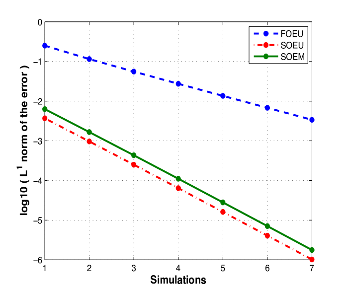
With this choice of model ingredients it can be easily verified that $\displaystyle p(s,t)=se^{t}$ is an exact solution of the DSSM. Given the exact solution, we can show numerically the order of accuracy of the schemes by means of an error table. We ran seven simulations for each scheme with step sizes being halved with each successive simulation. Then we calculated the corresponding $\displaystyle L^{1}$ norm of the error in each simulation for all schemes. In the initial simulation we let $\displaystyle N=10$ and $\displaystyle L=40$. Based on these consecutive $\displaystyle L_{1}$ errors we calculated the orders of accuracy, and listed the results in Table 1. This table indicates that the designed order of accuracy is obtained by all three schemes for this smooth solution of the model.

To have a better understanding of the order of accuracy, we plot the logarithmic value of the $\displaystyle L_{1}$ norm of the errors for all three schemes in Figure 1. Combining Table 1 and Figure 1, one can see clearly that the two second-order methods SOEU and SOEM perform almost equally well in this case when the model parameters and solutions are smooth functions. Also it seems that to get a similar accuracy as obtained in the second-order methods, the first-order method requires to adopt step sizes at least $\displaystyle 32$ times smaller.

Table 1: $\displaystyle L^{1}$ errors and orders of accuracy for FOEU, SOEU and SOEM schemes.

$\displaystyle N$	$\displaystyle L$	FOEU		SOEU		SOEM
		$\displaystyle L^{1}$ error	Order	$\displaystyle L^{1}$ error	Order	$\displaystyle L^{1}$ error	Order
10	40	2.51E-01		3.68E-03		6.30E-03
20	80	1.15E-01	1.12	9.63E-04	1.94	1.66E-03	1.92
40	160	5.56E-02	1.05	2.50E-04	1.95	4.33E-04	1.94
80	320	2.74E-02	1.02	6.39E-05	1.97	1.11E-04	1.97
160	640	1.36E-02	1.01	1.62E-05	1.98	2.81E-05	1.98
320	1280	6.78E-03	1.00	4.07E-06	1.99	7.07E-05	1.99
640	2560	3.39E-03	1.00	1.02E-06	2.00	1.77E-06	1.99

Figure 1: The logarithmic value of $\displaystyle L^{1}$ norm of the errors for FOEU, SOEU and SOEM schemes in seven simulations.

6.2 Behavior at discontinuity

The superiority of the SOEM scheme over both FOEU and SOEU methods is clear once solutions become discontinuous. To show this, we set the initial condition in the DSSM as

$$\begin{array}[]{ll}p^{0}(s)=\left\{\begin{array}[]{lll}0.5,&0\leq s<0.25,\\ 1,&0.25\leq s\leq 0.75,\\ 0.5,&0.75<s\leq 1,\\ \end{array}\right.\\ \end{array}$$

and choose the following model ingredients

$$\begin{array}[]{ll}\beta(s,y,Q)=\left\{\begin{array}[]{lll}0,&s\leq y-\frac{1}{2m},\\ m,&y-\frac{1}{2m}\leq s\leq y+\frac{1}{2m},\\ 0,&s>y+\frac{1}{2m},\end{array}\right.\\ \gamma(s,Q)=(1-s)/2,\\ \mu(s,Q)=2\exp(0.1Q),\\ \end{array}$$

with $\displaystyle m$ being a positive constant.
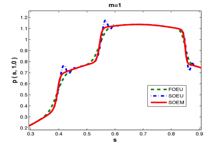
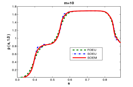
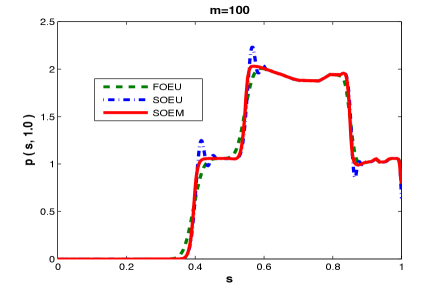
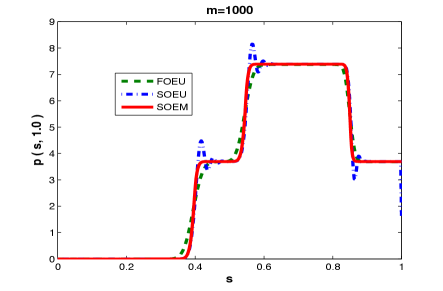
The above parameter choices introduce several discontinuities in the solution: two that arise from the initial condition and another that arises from the incompatibility of the boundary and initial condition at the origin. In the numerical simulations we use $\displaystyle T=1.0$, $\displaystyle N=400$, and $\displaystyle L=800$. The results corresponding to different values of $\displaystyle m$ for all three methods are shown in Figure 2. One can observe that SOEM scheme performs better than both the FOEU and SOEU schemes. It demonstrates sharper accuracy in capturing the discontinuity in the solution than both upwind schemes without generating (decaying) spurious oscillations.

Figure 2: The size distributions at time $\displaystyle t=1$ are plotted for all three schemes for $\displaystyle m=1,10,100$, and $\displaystyle 1000$.

6.3 Numerical verification of the convergence of solutions of DSSM to CSSM

In this section we provide some numerical corroboration to Theorem 5.1. To this end, we set the initial condition to be $\displaystyle p^{0}(s)=s^{3}$ and the parameters involved in the DSSM as follows:

$$\begin{array}[]{ll}\gamma(s,Q)=\frac{1}{2}(1-s),\\ \mu(s,Q)=1,\end{array}$$

To invoke Theorem 5.1 let

$$\beta_{1}(s,a,b)=\frac{s^{a-1}(1-s)^{b-1}}{B(a,b)},\quad s\in[0,1],$$

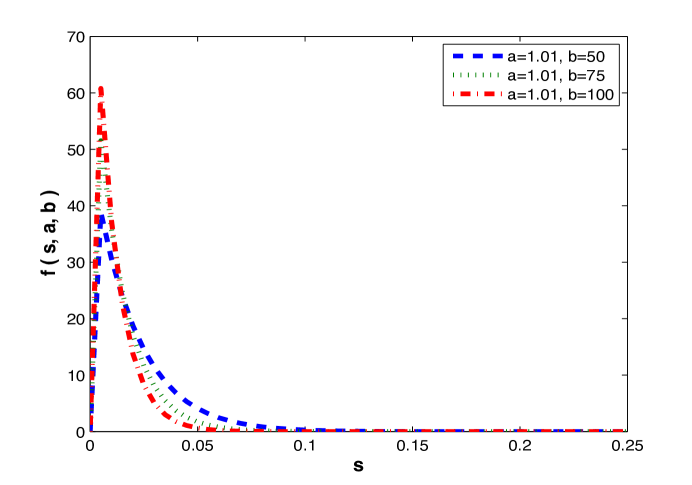
be the Beta probability density function with parameters $\displaystyle a$ and $\displaystyle b$; while

$$B(a,b)=\int_{0}^{1}x^{a-1}(1-x)^{b-1}\ dx$$

is the Beta function.

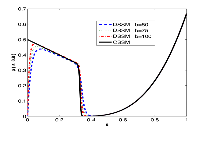
Note that if we fix $\displaystyle a>1$ and choose a sequence $\displaystyle b_{n}\to\infty$ then from the properties of the Beta probability density function the sequence of fertility functions of DSSM $\displaystyle\beta_{n}(s,y,Q)=\beta_{1}(s;a,b_{n})\beta_{2}(y,Q)$ with $\displaystyle\beta_{2}\equiv 1$ satisfies the conditions in Theorem 5.1. Thus, this theorem states that the solutions of the DSSM will converge to the solution of CSSM with fertility $\displaystyle\beta_{2}=1$ in the weak* topology. The numerical results we present below demonstrate that this convergence may actually hold in a stronger topology, namely $\displaystyle L^{1}$.

In the numerical simulations presented below, we choose $\displaystyle a=1.01$ and $\displaystyle b=50,75,100$, respectively. The graphs of the fertility function $\displaystyle\beta$ corresponding to these values of $\displaystyle b$ are shown in Figure 3. To simulate the CSSM, we let the fertility $\displaystyle\beta_{2}=1$ and for all other parameters we use the same values given above for DSSM. We then apply SOEM for solving the DSSM and CSSM. The results of the densities of DSSM and CSSM at $\displaystyle T=0.8$ are presented in Figure 4.

Figure 3: The graph of the distributed recruitment rate $\displaystyle\beta_{1}(s,a,b)$ for $\displaystyle a=1.01$ and $\displaystyle b=50,75,100$.

In Figure 4 we plot the solution $\displaystyle p$ at $\displaystyle t=0.8$ of the DSSM for different values of $\displaystyle b$, and the corresponding solution of the CSSM.

Figure 4: The solution $\displaystyle p(s,0.8)$ for DSSM corresponding to $\displaystyle a=1.01$ and $\displaystyle b=50,75,100$ against the solution $\displaystyle p(s,0.8)$ for CSSM.

6.4 Supercritical Hopf-bifurcation

We present a “toy model” here, in which a unique positive steady state looses its stability via Hopf-bifurcation. This example is further interesting, since as we will see, the net reproduction function is decreasing at the steady state (i.e. its derivative is negative) but the steady state is unstable. In fact this is the only case when stability can be lost via Hopf-bifurcation, since if the model ingredients are such that the derivative of the net reproduction function is positive then the governing linear semigroup is positive, see e.g. [11]. To illustrate the main ideas first we introduce a simple example for the classical Gurtin-MacCamy-type model, and then we perform numerical simulations to show that supercritical Hopf-bifurcation occurs in a corresponding distributed states-at-birth model, too.

Let $\displaystyle\gamma\equiv 1$ and the mortality rate $\displaystyle\mu=\mu(s)$. Assume that the survival probability $\displaystyle\pi(s)=\exp\left\{-\int_{0}^{s}\mu(\tau)d\tau\right\}$ is given by:

$$\begin{array}[]{ll}\pi(s)=\left\{\begin{array}[]{ll}1,&s\in[0,{s_{c}}],\\ 0,&s\in[{s_{c}},1],\end{array}\right.\end{array}$$ (6.2)

$$\begin{array}[]{ll}\beta(s,Q)=\left\{\begin{array}[]{ll}0,&s\in[0,q)\cup(q+\varepsilon,1],\,Q\in[0,\infty),\\ e^{-Q}\tilde{R}\varepsilon^{-1},&s\in[q,q+\varepsilon],\,Q\in[0,\infty),\end{array}\right.\end{array}$$ (6.3)

where $\displaystyle\tilde{R}>1,\,\varepsilon>0$, and $\displaystyle 0<q<{s_{c}}<1$. Note that in this example both the fertility and mortality functions are discontinuous. With this choice of the survival probability and fertility function the net reproduction function reads:

$$R(Q)=\int_{q}^{q+\varepsilon}e^{-Q}\tilde{R}\varepsilon^{-1}\,ds=\tilde{R}e^{-Q}.$$

Hence for any $\displaystyle\tilde{R}>1$ there is a unique positive steady state with total population size $\displaystyle Q_{*}=\ln(\tilde{R})$. We have

$$p_{*}(0)=\frac{Q_{*}}{\int_{0}^{1}\pi(s)\,ds}={s_{c}}^{-1}\ln(\tilde{R}),\quad\text{and}\quad p_{*}(s)={s_{c}}^{-1}\ln(\tilde{R})\pi(s).$$

The characteristic equation corresponding to the linearized system at the positive steady state reads (see e.g. [11]):

$$\displaystyle 1=K(\lambda) \displaystyle=\int_{0}^{1}\beta(s,Q_{*})\pi(s)e^{-\lambda s}\,ds$$

$$\displaystyle\quad+\int_{0}^{1}\pi(s)e^{-\lambda s}\,ds\int_{0}^{1}{s_{c}}^{-1}\ln(R)\beta_{Q}(s,Q_{*})\pi(s)\,ds$$

$$\displaystyle=e^{-\lambda q}\frac{1-e^{-\lambda\varepsilon}}{\lambda\varepsilon}-{s_{c}}^{-1}\ln(\tilde{R})\frac{1-e^{-\lambda{s_{c}}}}{\lambda}.$$ (6.4)

In the limit as $\displaystyle\varepsilon\to 0$ the characteristic equation (6.4) reduces to:

$$1=e^{-\lambda q}-{s_{c}}^{-1}\ln(\tilde{R})\frac{1-e^{-\lambda{s_{c}}}}{\lambda}.$$ (6.5)

We look first for pure imaginary roots of the characteristic equation (6.5), i.e. assume that $\displaystyle\lambda=i\alpha$ for some $\displaystyle\alpha\in\mathbb{R}\setminus\{0\}$. For such an eigenvalue equation (6.5) reads:

$$1=(\cos(\alpha q)-i\sin(\alpha q))+i\alpha^{-1}{s_{c}}^{-1}\ln(\tilde{R})(1-\cos(\alpha{s_{c}})+i\sin(\alpha{s_{c}})),$$ (6.6)

which is equivalent to

$$\displaystyle 1= \displaystyle\cos(\alpha q)-\alpha^{-1}{s_{c}}^{-1}\ln(\tilde{R})\sin(\alpha{s_{c}}),$$ (6.7)

$$\displaystyle 0= \displaystyle-\sin(\alpha q)-\alpha^{-1}{s_{c}}^{-1}\ln(\tilde{R})(\cos(\alpha{s_{c}})-1).$$ (6.8)

Straightforward calculations show that for $\displaystyle q=\frac{1}{6},\,{s_{c}}=\frac{1}{2}$ and for $\displaystyle\ln(\tilde{R})=\frac{3\pi}{2}$ equations (6.7)-(6.8) admit the solution $\displaystyle\lambda=3\pi i$. Next we would like to show that the pair of purely imaginary eigenvalues $\displaystyle\lambda_{1/2}=\pm 3\pi i$ cross the $\displaystyle y$-axis to the right. To this end we write $\displaystyle{s_{c}}^{-1}\ln(\tilde{R})=3\pi+r$ and $\displaystyle\lambda=q+3\pi i$, where $\displaystyle r,q\in\mathbb{R}$. The characteristic equation (6.5) reads:

$$1=-ie^{-\frac{q}{6}}-\frac{r+3\pi}{q+3\pi i}(1-ie^{-\frac{r}{2}}),$$

which leads to

$$\displaystyle 3\pi= \displaystyle-qe^{-\frac{q}{6}}+(r+3\pi)e^{-\frac{r}{2}},$$

$$\displaystyle q= \displaystyle 3\pi e^{-\frac{q}{6}}-r-3\pi\Rightarrow r+3\pi=3\pi e^{-\frac{q}{6}}-q.$$

Hence for $\displaystyle r<0\,(\iff{s_{c}}>0.5)$ small enough the eigenvalue $\displaystyle\lambda=q+3\pi i$ with have a positive real part. Next we note that the continuous dependence of the eigenvalues on the parameter $\displaystyle\varepsilon$ (see e.g. [12, Ch.IV.3.5]) implies that for $\displaystyle\varepsilon>0$ small enough the eigenvalue will still have a positive real part.

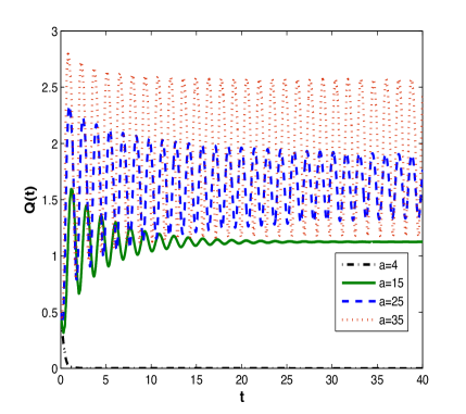
Our next numerical example demonstrates, for the first time as far as we know, that such bifurcation may also occur in the DSSM. This is somewhat surprising mainly because the integral operator representing the distributed states-at-birth may have a smoothing effect, in general. We let $\displaystyle p^{0}=s$ and

$$\begin{array}[]{ll}\gamma=1,\\ \mu=\frac{160}{(250000s^{2}-250000s+62505)(0.32\arctan(250-500s)+2)},\\ \beta=\beta_{1}(s,Q)\beta_{2}(y),\end{array}$$

where

$$\begin{array}[]{ll}\beta_{1}(s,Q)=a\exp(-Q)\left(10\arctan(5-1000s)+15.7\right),\\ \beta_{2}(y)=\frac{1}{\sqrt{2\pi}}\exp{\left(-0.5\left(100(y-1/6+0.005)\right)^{2}\right)}\exp\left(\frac{3\pi}{2}\right).\end{array}$$

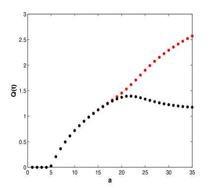
Here $\displaystyle a$ is a positive constant. The dynamics of total population $\displaystyle Q(t)$ for different values of $\displaystyle a$ are shown in Figure 5. Only the maximum and minimum values of $\displaystyle Q$ are plotted in the bifurcation graph of the dynamics of $\displaystyle Q(t)$ with respect to $\displaystyle a$ .

Figure 5: Left: A comparison of the total population sizes $\displaystyle Q(t)$ for $\displaystyle a=6,26,46$; Right: Bifurcation graph of $\displaystyle Q$ with respect to parameter $\displaystyle a$.

7 Conclusion

We have developed a first order upwind scheme and a second order finite difference scheme to approximate the solution of a size-structured population model with distributed states-at-birth. Convergence of both schemes to the unique bounded total variation weak solution has been proved. Numerical results are provided to demonstrate the capability of the numerical methods in resolving smooth as well as discontinuous solutions. For smooth solutions both schemes achieve the designed order of accuracy. For discontinuous solutions, the second order scheme demonstrates better accuracy in capturing the discontinuity compared to upwind schemes. The second order scheme is also applied to the distributed states-at-birth model (DSSM) to show that supercritical Hopf-bifurcation may occur in such models.

We also proved the convergence of the weak solution for the distributed size-structured model (DSSM) in the weak* topology to that of the classical size-structured model (CSSM) under certain conditions on the fertility function and used the second order scheme to demonstrate this convergence.

Acknowledgements: The work of A.S. Ackleh, X. Li and B. Ma is partially supported by the National Science Foundation under grant # DMS-1312963. J. Z. Farkas was supported by a University of Stirling research and enterprise support grant.

References

- [1] A.S. Ackleh, K. Deng and J. Thibodeaux, A monotone approximation for a size-structured population model with a generalized environment, J. Biol. Dyn., 1 (2007), 291-304.
- [2] A.S. Ackleh and J.Z. Farkas, On the net reproduction rate of continuous structured populations with distributed states at birth, Comput. Math. Appl., 66 (2013), 1685-1694.
- [3] A.S. Ackleh and B.G. Fitzpatrick, Modeling aggregation and growth processes in an algal population model: analysis and computations, J. Math. Biol., 35 (1997), 480-502.
- [4] A. S. Ackleh and K. Ito, An implicit finite difference scheme for the nonlinear size-structured population model, Numer. Funct. Anal. Optim., 18 (1997), 865-884.
- [5] A.S. Ackleh and B. Ma, A second order high resolution scheme for a juvenile-adult model of amphibians, Numer. Funct. Anal. Optim., 34 (2013), 365-403.
- [6] Azmy S. Ackleh, B. Ma and Jeremy J. Thibodeaux, A second-order high resolution finite difference scheme for a structured erythropoiesis model subject to malaria infection, Math. Biosci., 245 (2013), 2-11.
- [7] A. Calsina and J. Saldana, Basic theory for a class of models of hierarchically structured population dynamics with distributed states in the recruitment, Math. Model. Meth. Appl. Sci., 16 (2006), 1695-1722.
- [8] J.M. Cushing, An Introduction to Structured Population Dynamics, SIAM, Philadelphia, 1998.
- [9] J.M. Cushing, Some competition models for size-structured populations, Rocky Mountain J. Math., 20 (1990), 879-897.
- [10] J. Z. Farkas, D. M. Green and P. Hinow, Semigroup analysis of structured parasite populations, Math. Model. Nat. Phenom., 5 (2010), 94-114.
- [11] J. Z. Farkas and T. Hagen, Stability and regularity results for a size-structured population model, J. Math. Anal. Appl., 328 (2007), 119-136.
- [12] T. Kato, Perturbation Theory for Linear Operators, Springer, Berlin Heidelberg, 1995.
- [13] Ph. Laurencot and S. Mischler, Global existence for the discrete diffusive coagulation-fragmentation equation in L1, Rev. Mat. Iberoamericana, 18 (2002), 731-745.
- [14] R. J. LeVeque, Numerical Methods for Conservation Laws, Birkhauser Verlag, Basel, 1990.
- [15] J. Metz and O. Diekmann, The Dynamics of Physiologically Structured Populations Lecture Notes in Biomath. 68, Springer-Verlag, Berlin, 1986.
- [16] D. McLaughlin, W. Lamb and A. McBride, An existence and uniqueness result for a coagulation and multiple-fragmentation equation, SIAM J. Math. Anal., 28 (1997), 1173-1190.
- [17] S. V. Patankar, Numerical Heat Transfer and Fluid Flow, Taylor & Francis, ISBN 978-0-89116-522-4, 1980.
- [18] J. Shen, C.-W. Shu and M. Zhang, High resolution schemes for a hierarchical size-structured model, SIAM. J. Numer. Anal., 45 (2007), 352-370.
- [19] J. Smoller, Shock Waves and Reaction-Diffusion Equation, Springer-Verlag, New York, 2007.
- [20] S. Tucker and S. Zimmerman, A nonlinear model of population dynamics containing an arbitrary number of continuous structure variables, SIAM J. Appl. Math., 48 (1988), 594-591.
- [21] D. Wrzosek, Existence of solutions for the discrete coagulation-fragmentation model with diffusion, Topol. Meth. Nonlinear Anal., 9 (1997), 279-296.
- [22] R. Xu, Z. Ma and Q. Gan, Stability and bifurcation in a Beddington-DeAngelis type predator-prey model with prey dispersal, Rocky Mountain J. Math., 38 (2008), 1761-1783.