Reflecting about Selecting Noninformative Priors

Abstract

Following the critical review of Seaman III et al (2012), we reflect on what is presumably the most essential aspect of Bayesian statistics, namely the selection of a prior density. In some cases, Bayesian inference remains fairly stable under a large range of noninformative prior distributions. However, as discussed by Seaman III et al (2012), there may also be unintended consequences of a choice of a noninformative prior and, these authors consider this problem ignored in Bayesian studies. As they based their argumentation on four examples, we reassess these examples and their Bayesian processing via different prior choices. Our conclusion is to lower the degree of worry about the impact of the prior, exhibiting an overall stability of the posterior distributions. We thus consider that the warnings of Seaman III et al (2012), while commendable, do not jeopardize the use of most noninformative priors.

1 Introduction

The choice of a particular prior for the Bayesian analysis of a statistical model is often seen more as an art than as a science. When the prior cannot be derived from the available information, it is generaly constructed as a noninformative prior. This derivation is mostly mathematical and, even though the corresponding posterior distribution has to be proper and hence constitutes a correct probability density, it nonetheless leaves the door open to criticism. The focus of this note is the paper by Seaman III et al (2012), where the authors consider using a particular noninformative distribution as a problem in itself, often bypassed by users of these priors: “if parameters with diffuse proper priors are subsequently transformed, the resulting induced priors can, of course, be far from diffuse, possibly resulting in unintended influence on the posterior of the transformed parameters” (p.77). Using the inexact argument that most problems rely on MCMC methods and hence require proper priors, the authors restrict the focus to those priors.

In their critical study, Seaman III et al (2012) investigate the negative side effects of some specific prior choices related with specific examples. Our note aims at re-examining their investigation and at providing a more balanced discussion on these side effects. We first stress that a prior is considered as informative by Seaman III et al (2012) “to the degree it renders some values of the quantity of interest more likely than others” (p.77), and with this definition, when comparing two priors, the prior that is more informative is deemed preferable. In contrast with this definition, we consider that an informative prior expresses specific, definite (prior) information about the parameter, providing quantitative information that is crucial to the estimation of a model through restrictions on the prior distribution (Robert, 2007). However, in most practical cases, a model parameter has no substance per se but instead calibrates the probability law of the random phenomenon observed therein. The prior is thus a tool that summarizes the information available on this phenomenon, as well as the uncertainty within the Bayesian structure. Many discussions can be found in the literature on how appropriate choices between the prior distributions can be decided. In this case, robustness considerations also have an important role to play (Lopes and Tobias, 2011; Stojanovski and Nur, 2011). This point of view will be obvious in this note as, e.g., in processing a logistic model in the following section. Within the sole setting of the examples first processed in Seaman III et al (2012), we do exhibit a greater stability in the posterior distributions through various noninformative priors.

The plan of the note is as follows: we first provide a brief review of noninformative priors in Section 2. In Section 3, we propose a Bayesian analysis of a logistic model (Seaman III et al.’s (2012) first example) by choosing the normal distribution $N(0,\sigma^{2})$ as the regression coefficient prior. We then compare it with a $g$-prior, as well as flat and Jeffreys’ priors, concluding to the stability of our results. The next sections cover the second to fourth examples of Seaman III et al (2012), modeling covariance matrices, treatment effect in biomedical studies, and a multinomial distribution. When modeling covariance matrices, we compare two default priors for the standard deviations of the model coefficients. In the multinomial setting, we discuss the hyperparameters of a Dirichlet prior. Finally, we conclude with the argument that the use of noninformative priors is reasonable within a fair range and that they provide efficient Bayesian estimations when the information about the parameter is vague or very poor.

2 Noninformative priors

As mentioned above, when prior information is unavailable and if we stick to Bayesian analysis, we need to resort to one of the so-called noninformative priors. Since we aim at a prior with minimal impact on the final inference, we define a noninformative prior as a statistical distribution that expresses vague or general information about the parameter in which we are interested. In constructive terms, the first rule for determining a noninformative prior is the principle of indifference, using uniform distributions which assign equal probabilities to all possibilities (Laplace, 1820). This distribution is however not invariant under reparametrization (see Berger, 1980; Robert, 2007, for references). If the problem does not allow for an invariance structure, Jeffreys’ (1939) priors, then reference priors, exploit the probabilistic structure of the problem under study in a more formalised way. Other methods have been advanced, like the little-known data-translated likelihood of Box and Tiao (2011), maxent priors (Jaynes, 2003), minimum description length priors (Rissanen, 2012) and probability matching priors (Welch and Peers, 1963).

Bernardo and Smith (2009) envision noninformative priors as a mere mathematical tool, while accepting their feature of minimizing the impact of the prior selection on inference: “Put bluntly, data cannot ever speak entirely for themselves, every prior specification has some informative posterior or predictive implications and vague is itself much too vague an idea to be useful. There is no “objective” prior that represents ignorance” (p.298). There is little to object against this quote since, indeed, prior distributions can never be quantified or elicited exactly, especially when no information is available on those parameters. Hence, the concept of “true” prior is meaningless and the quantification of prior beliefs operates under uncertainty. As stressed by Berger (1984), noninformative priors enjoy the advantage that they can be considered to provide robust solutions to relevant problems even though “the user of these priors should be concerned with robustness with respect to the class of reasonable noninformative priors” (p.59).

3 Example 1: Bayesian analysis of the logistic model

The first example in Seaman III et al (2012) is a standard logistic regression modelling the probability of coronary heart disease as dependent on the age $x$ by

$$\rho(x)=\frac{\mathrm{exp}{(\alpha+\beta x)}}{1+\mathrm{exp}{(\alpha+\beta x)}}.$$ (1)

First we recall the original discussion in Seaman III et al (2012) and then run our own analysis by selecting some normal priors as well as the $g$-prior, the flat prior and Jeffreys’ prior.

3.1 Seaman et al.’s (2012) analysis

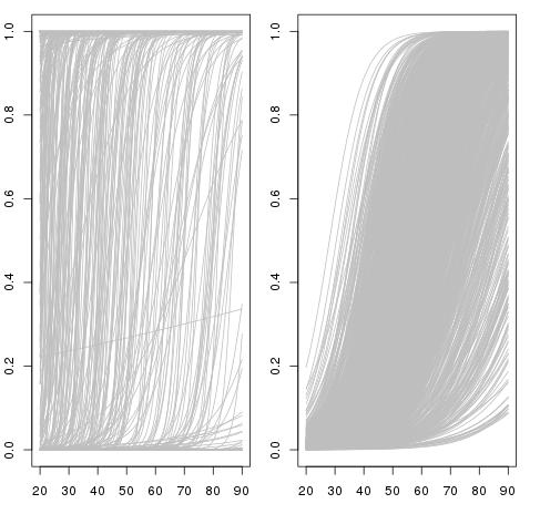
For both parameters of the model (1), Seaman III et al (2012) chose a normal prior $N(0,\sigma^{2})$. A first surprising feature in this choice is to opt for an identical prior on both intercept and slope coefficients, instead of, e.g., a $g$-prior (discussed in the following) that would rescale each coefficient according to the variation of the corresponding covariate. Indeed, since $x$ corresponds to age, the second term $\beta x$ in the regression varies $50$ times more than the intercept. When plotting logistic cdf’s induced by a few thousands simulations from the prior, those cumulative functions mostly end up as constant functions with the extreme values $0$ and $1$. This behaviour is obviously not particularly realistic since the predicted phenomenon is the occurrence of coronary heart disease. Under this minimal amount of information, the prior is thus using the wrong scale: the simulated cdfs should have a reasonable behavior over the range $(20,100)$ of the covariate $x$. For instance, it should focus on a $-5$ log-odds ratio at age $20$ and a $+5$ log-odds ratio at $100$, leading to the comparison pictured in Figure 1 (left versus right). Furthermore, the fact that the coefficient of $x$ may be negative also bypasses a basic item of information about the model and answers the later self-criticism in Seaman III et al (2012) that the prior probability that the ED50 is negative is $0.5$. Using instead a flat prior would answer the authors’ criticisms about the prior behavior, as we now demonstrate.

Figure 1: Logistic cdfs across a few thousans simulations from the normal prior, when using the prior selected by Seaman III et al (2012) (left) and the prior defined as the $G$-prior(right)

We stress that Seaman III et al (2012) produce no further justification for the choice of the prior variance $\sigma^{2}=25^{2}$, other than there is no information about the model parameters. This is a completely arbitrary choice of prior, arbitrariness that does have a considerable impact on the resulting inference, as already discussed. Seaman III et al (2012) further criticized the chosen prior by comparing both posterior mode and posterior mean derived from the normal prior assumption with the MLE. If the MLE is the golden standard there then one may wonder about the relevance of a Bayesian analysis! When the sample size $N$ gets large, most simple Bayesian analyses based on noninformative prior distributions give results similar to standard non-Bayesian approaches (Gelman et al, 2013). For instance, we can often interpret classical point estimates as exact or approximate posterior summaries based on some implicit full probability model. Therefore, as $N$ increases, the influence of the prior on posterior inferences decreases and, when $N$ goes to infinity, most priors lead to the same inference. However, for smaller sample sizes, it is inappropriate to summarize inference about the parameter by one value like the mode or the mean, especially when the posterior distribution of the parameter is more variable or even asymmetric.

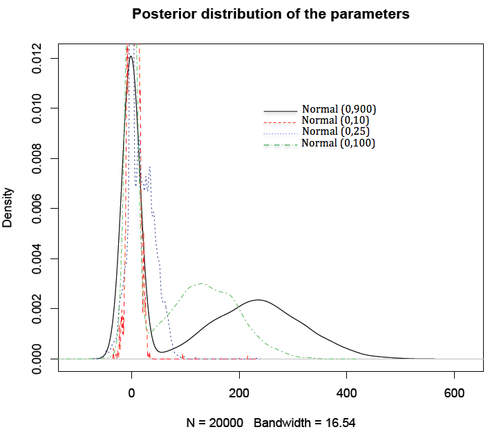
The dataset used here to infer on $(\alpha,\beta)$ is the Swiss banknote benchmark (available in R). The response variable $y$ indicates the state of the banknote, i.e. whether the bank note is genuine or counterfeit. The explanatory variable is the bill length. This data yields the maximum likelihood estimates $\tilde{\alpha}=233.26$ and $\tilde{\beta}=-1.09$. To check the impact of the normal prior variance, we used a random walk Metropolis-Hastings algorithm as in Marin and Robert (2007) and derived the estimators reproduced in Table 1. We can spot definitive changes in the results that are caused by moves in the coefficient $\sigma$, hence concluding to the clear sensitivity of the posterior to the choice of hyperparameter $\sigma$ (see also Figure 2).

Table 1: Posterior estimates of the logistic parameters using a normal prior when $\sigma=10,25,100,900$

$\sigma=10$ $\hat{\alpha}$ $\hat{\beta}$ mean s.d mean s.d 3.482 11.6554 -0.0161 0.0541 $\sigma=25$ 18.969 24.119 -0.0882 0.1127 $\sigma=100$ 137.63 64.87 -0.6404 0.3019 $\sigma=900$ 237.2 86.12 -1.106 0.401

Figure 2: Posterior distributions of the logistic parameter $\alpha$ when priors are $N(0,\sigma)$ for $\sigma=10,25,100,900$, based on $10^{4}$ MCMC simulations.

3.2 Larger classes of priors

Normal priors are well-know for their lack of robustness (see e.g. Berger, 1984) and the previous section demonstrates the long-term impact of $\sigma$. However, we can limit variations in the posteriors, using the $g$-priors of Zellner (1986),

$$\alpha,\beta\mid X\sim N_{2}(0,g(X^{T}X)^{-1}).$$ (2)

where the prior variance-covariane matrix is a scalar multiple of the information matrix for the linear regression. This coefficient $g$ plays a decisive role in the analysis, however large values of $g$ imply a more diffuse prior and, as shown e.g. in Marin and Robert (2007), if the value of $g$ is large enough, the Bayes estimate stabilizes. We will select $g$ as equal to the sample size $200$, following Liang et al (2008), as it means that the amount of information about the parameter is equal to the amount of information contained in one single observation.

A second reference prior is the flat prior $\pi(\alpha,\beta)=1$. And Jeffreys’ prior constitutes our third prior as in Marin and Robert (2007). In the logistic case, Fisher’s information matrix is $\mathbf{I}(\alpha,\beta,X)=X^{T}WX$, where $X=\{x_{ir}\}$ is the design matrix, $W=\mathrm{diag}\{m_{i}\pi_{i}(1-\pi_{i})\}$ and $m_{i}$ is the binomial index for the ith count (Firth, 1993). This leads to Jeffreys’ prior $\{\mathrm{det}(\mathbf{I}(\alpha,\beta,X))\}^{\nicefrac{{1}}{{2}}}$, proportional to

$$\left[\sum_{i=1}^{n}\frac{\mathrm{exp}{(\alpha+\beta x_{i})}}{\{1+\mathrm{exp}{(\alpha+\beta x_{i})}\}^{2}}\sum_{i=1}^{n}\frac{x_{i}^{2}\mathrm{exp}{(\alpha+\beta x_{i})}}{\{1+\mathrm{exp}{(\alpha+\beta x_{i})}\}^{2}}-\left\{\sum_{i=1}^{n}\frac{x_{i}\mathrm{exp}{(\alpha+\beta x_{i})}}{\{1+\mathrm{exp}{(\alpha+\beta x_{i})}\}^{2}}\right\}^{2}\right]^{\frac{1}{2}}$$

This is a nonstandard distribution on $(\alpha,\beta)$ but it can be easily approximated by a Metropolis-Hastings algorithm whose proposal is the normal Fisher approximation of the likelihood, as in Marin and Robert (2007).

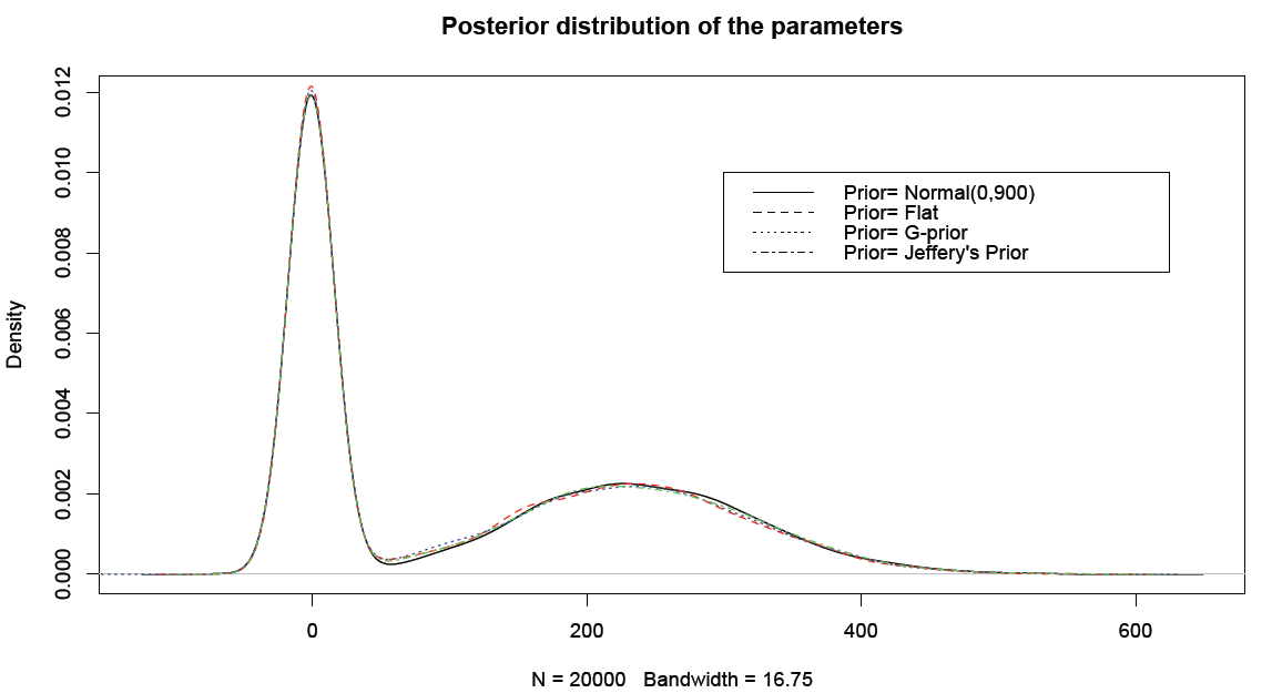
Bayesian estimates of the regression coefficients associated with the above three noninformative priors are summarized in Table 2. Those estimates vary quite moderately from one choice to the next, as well as relatively to the MLEs and to the results shown in Table 1 when $\sigma=900$. Figure 3 is even more definitive about this stability of Bayesian inferences under different noninformative prior choices.

Table 2: Posterior estimates of the logistic parameters under a $g$-prior, a flat prior and Jeffreys’ prior for the banknote benchmark. Posterior means and standard deviations remain quite similar under all priors. All point estimates are averages of MCMC samples of size $10^{4}$.

$g$-prior $\hat{\alpha}$ $\hat{\beta}$ mean s.d mean s.d 237.63 88.0377 -1.1058 0.4097 Flat prior 236.44 85.1049 -1.1003 0.3960 Jeffreys’ prior 237.24 87.0597 -1.1040 0.4051

Figure 3: Posterior distributions of the parameters of the logistic model when the prior is $N(0,900^{2})$, g-prior, flat prior and Jeffreys’ prior, respectively. The estimated posterior distributions are based on $10^{4}$ MCMC iterations.

4 Example 2: Modeling covariance matrices

The second choice of prior criticized by Seaman III et al (2012), was proposed by Barnard et al (2000) for the modeling of covariance matrices. However the paper falls short of demonstrating a clear impact of this prior modelling on posterior inference. Furthermore the adeopted solution of using another proper prior resulting in a “wider” dispersion requires a prior knowledge of how wide is wide enough. We thus run Bayesian analyses considering prior beliefs specified by both Seaman III et al (2012) and Barnard et al (2000).

4.1 Setting

The multivariate regression model of Barnard et al (2000) is

$$Y_{j}\mid X_{j},\beta_{j},\tau_{j}\sim N(X_{j}\beta_{j},\tau_{j}^{2}I_{n_{j}}),~{}~{}j=1,2,\ldots,m.$$ (3)

where $Y_{j}$ is a vector of $n_{j}$ dependent variables, $X_{j}$ is an $n_{j}\times k$ matrix of covariate variables, and $\beta_{j}$ is a $k$-dimensional parameter vector. For this model, Barnard et al (2000) considered an iid normal distribution as the prior

$$\beta_{j}\sim N(\bar{\beta},\Sigma)$$

conditional on $\bar{\beta},\Sigma$ where $\bar{\beta},\tau_{j}^{2}$ for $j=1,2,\ldots,m$ are independent and follow a normal and inverse-gamma priors, respectively. Assuming that $\bar{\beta},\tau_{j}^{2}$’s and $\Sigma$ are a priori independent, Barnard et al (2000) firstly provide a full discussion on how to choose a prior for $\Sigma$ because it determines the nature of the shrinkage of the posterior of the individual $\beta_{j}$ is towards a common target. The covariance matrix $\Sigma$ is defined as a diagonal matrix with diagonal elements $S$, multiplied by a $k\times k$ correlation matrix $R$,

$$\Sigma=\mathrm{diag}(S)R\mathrm{diag}(S)\,.$$

Note that $S$ is the $k\times 1$ vector of standard deviations of the $\beta_{j}$s, $(S_{1},\ldots,S_{k})$. Barnard et al (2000) propose lognormal distributions as priors on $S_{j}$. The correlation matrix could have (1) a joint uniform prior $p(R)\propto 1$, or (2) a marginal prior obtained from the inverse-Wishart distribution for $\Sigma$ which means $p(R)$ is derived from the integral over $S_{1},\ldots,S_{k}$ of a standard inverse-Wishart distribution. In the second case, all the marginal densities for $r_{ij}$ are uniform when $i\neq j$ (Barnard et al, 2000).

Considering the case of a single regressor, i.e. $k=2$, Seaman III et al (2012) chose a different prior structure, with a flat prior on the correlations and a lognormal prior with means $1$ and $-1$, and standard deviations $1$ and $0.5$ on the standard deviations of the intercept and slope, respectively. Simulating from this prior, they concluded at a high concentration near zero. They then suggested that the lognormal distribution should be replaced by a gamma distribution $G(4,1)$ as it implies a more diffuse prior. The main question here is whether or not the induced prior is more diffuse should make us prefer gamma to lognormal as a prior for $S_{j}$, as discussed below.

4.2 Prior beliefs

First, Barnard et al.’s (2000) basic modeling intuition is “that each regression is a particular instance of the same type of relationship” (p.1292). This means an exchangeabile prior belief on the regression parameters. As an example, they suppose that $m$ regressions are similar models where each regression corresponds to a different firm in the same industry branch. Exploiting this assumption, when $\beta_{j}$ has a normal prior like $\beta_{ij}\sim N(\bar{\beta}_{i},\sigma_{i}^{2}),\ j=1,2,\ldots,m$, the standard deviation of $\beta_{ij}$ ($S_{i}=\sigma_{i}$) should be small as well so “that the coefficient for the $i$th explanatory variable is similar in the different regressions” (p.1293). In other words, $S_{i}$ concentrated on small values implies little variation in the $i$th coefficient. Toward this goal, Barnard et al (2000) chose a prior concentrated close to zero for the standard deviation of the slope so that the posterior of this coefficient would be shrunken together across the regressions. Based on this basic idea and taking tight priors on $\Sigma$ for $\beta_{j},j=1,\ldots,m$, they investigated the shrinkage of the posterior on $\beta_{j}$ as well as the degree of similarity of the slopes. Their analysis showed that a standard deviation prior that is more concentrated on small values results in substantial shrinkage in the coefficients relative to other prior choices.

Consider for instance the variation between the choices of lognormal and gamma distributions as priors of $S_{2}$, standard deviation of the regression slope. Figure 4 compares the lognormal prior with mean $-1$ and standard deviation $0.5$ and the gamma distribution ${G}(4,1)$.

Figure 4: Comparison of lognormal and gamma priors for the standard deviation of the regression slope.

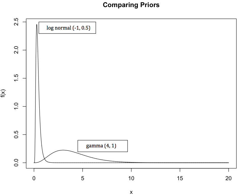
In this case, most of the mass of the lognormal prior is concentrated on values close to zero whereas the gamma prior is more diffuse. The $10,50,90$ percentiles of $LN(-1,0.5)$ and $G(4,1)$ are $0.19,0.37,0.7$ and $1.74,3.67,6.68$, respectively. Thus, choosing $LN(-1,0.5)$ as the prior of $S_{2}$ is equivalent to believe that values of $\beta_{2}$ in the $m$ regressions are much closer together than the situation where we assume $S_{2}\sim G(4,1)$. To assess the difference between both prior choices on $S_{2}$ and their impact on the degree of similarity of the regression coefficients, we resort to a simulated example, similar to Barnard et al (2000), except that $m=4$ and $n_{j}=36$. The explanatory variables are simulated standard normal variates. We also take $\tau_{j}\sim IG(3,1)$ and $\bar{\beta}\sim N(0,1000I)$. The prior for $\Sigma$ is such that $\pi(R)\propto 1$ and we run Seaman et al.’s (2012) analyses under $S_{2}\sim LN(-1,0.5)$ and $S_{2}\sim G(4,1)$.

4.3 Comparison of posterior outputs

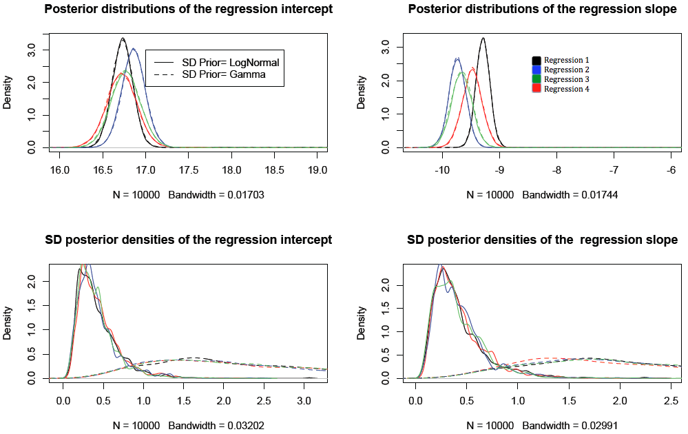
As seen in Tables 3 and 4, respectively. The differences between the regression estimates are quite limited from one prior to the next, while the estimates of the standard deviations vary much more. In the lognormal case, the posterior of $S_{i}$ is concentrated on smaller values relative to the gamma prior. Figure 5 displays the posterior distributions of those parameters. the impact of the prior choice is quite clear on the standard deviations. Therefore, since the posteriors of both intercepts and slopes for all four regressions are centered in $(16.5,17)$ and $(-10,-9)$, respectively, we can conclude at the stability of Bayesian inferences on $\beta_{j}$ when selecting two different prior distributions on $S_{j}$. That the posteriors on the $S_{i}$’s differ is in fine natural since those are hyperparameters that are poorly informed by the data, thus reflecting more the modelling choices of the experimenter.

Table 3: Posterior estimations of regression coefficients when their standard deviations are distributed as $LN(-1,0.5)$ and $G(4,1)$.

$S_{i}\sim LN(-1,0.5)$ Regression 1 Regression 2 Regression 3 Regression 4 Estimate mean s.d mean s.d mean s.d mean s.d Intercept 16.74 0.17 16.72 0.17 16.79 1.09 16.82 0.69 Slope -9.27 0.42 -9.47 0.25 -9.66 0.98 -9.63 0.45 $S_{i}\sim G(4,1)$ Regression 1 Regression 2 Regression 3 Regression 4 Estimate mean s.d mean s.d mean s.d mean s.d Intercept 16.73 0.23 16.73 0.22 16.85 0.37 16.76 0.32 Slope -9.30 0.30 -9.47 0.34 -9.73 0.23 -9.64 0.80

Table 4: Posterior estimations standard deviations of the regression coefficients when their priors are distributed as $LN(-1,0.5)$ versus $G(4,1)$.

$S_{i}\sim LN(-1,0.5)$ Regression 1 Regression 2 Regression 3 Regression 4 Estimate mean s.d mean s.d mean s.d mean s.d $S_{1}$ 0.43 0.27 0.44 0.26 0.42 0.26 0.41 0.24 $S_{2}$ 0.42 0.27 0.43 0.25 0.42 0.25 0.43 0.32 $S_{i}\sim G(4,1)$ Regression 1 Regression 2 Regression 3 Regression 4 Estimate mean s.d mean s.d mean s.d mean s.d $S_{1}$ 2.31 1.28 2.33 1.29 2.29 1.29 2.29 1.26 $S_{2}$ 2.32 1.29 2.23 1.28 2.25 1.23 2.30 1.26

Figure 5: Estimated posterior densities of the regression intercept (top left), slope (top right), standard deviation of the intercept (down left) and standard deviation of the slope (down right), respectively for $4$ different normal regressions. All estimates based on $10^{5}$ iterations that were simulated from a Gibbs sampler.

5 Examples 3 and 4: Prior choices for a proportion and the multinomial coefficients

This section considers more briefly the third and fourth examples of Seaman III et al (2012). The third example relates to a treatment effect analyzed by Cowles (2002) and the fourth one covers a standard multinomial setting.

5.1 Proportion of treatment effect captured

In Cowles (2002) two models are compared for surrogate endpoints, using a link function $g$ that either includes the surrogate marker or not. The quantity of interest is a proportion of treatment effect captured: it is defined as $\mathrm{PTE}\equiv 1-{\beta_{1}}/{\beta_{R,1}}$, where $\beta_{1},\beta_{R,1}$ are the coefficients of an indicator variable for treatment in the first and second regression models under comparison, respectively. Seaman III et al (2012) restricted this proportion to the interval $(0,1)$ and under this assumption they proposed to use a generalised beta distribution on $\beta_{1},\beta_{R,1}$ so that $\mathrm{PTE}$ stayed within $(0,1)$.

We find this example most intringuing in that, even if PTE could be turned into a meaningful quantity (given that it depends on parameters from different models), the criticism that it may take values outside $(0,1)$ is rather dead-born since it suffices to impose a joint prior that ensures the ratio stays within $(0,1)$. This actually is the solution eventually proposed by the authors. If we have prior beliefs about the parameter space (which depends on ${\beta_{1}}/{\beta_{R,1}}$ in this example) the prior specified on the quantity of interest should integrate these beliefs. In the current setting, there is seemingly no prior information about $(\beta_{1},\beta_{R,1})$ and hence imposing a prior restriction to $(0,1)$ is not a logical specification. For instance, using normal priors on $\beta_{1}$ and $\beta_{R,1}$ lead to a Cauchy prior on ${\beta_{1}}/{\beta_{R,1}}$, which support is not limited to $(0,1)$. We will not discuss this rather artificial example any further.

5.2 Multinomial model and evenness index

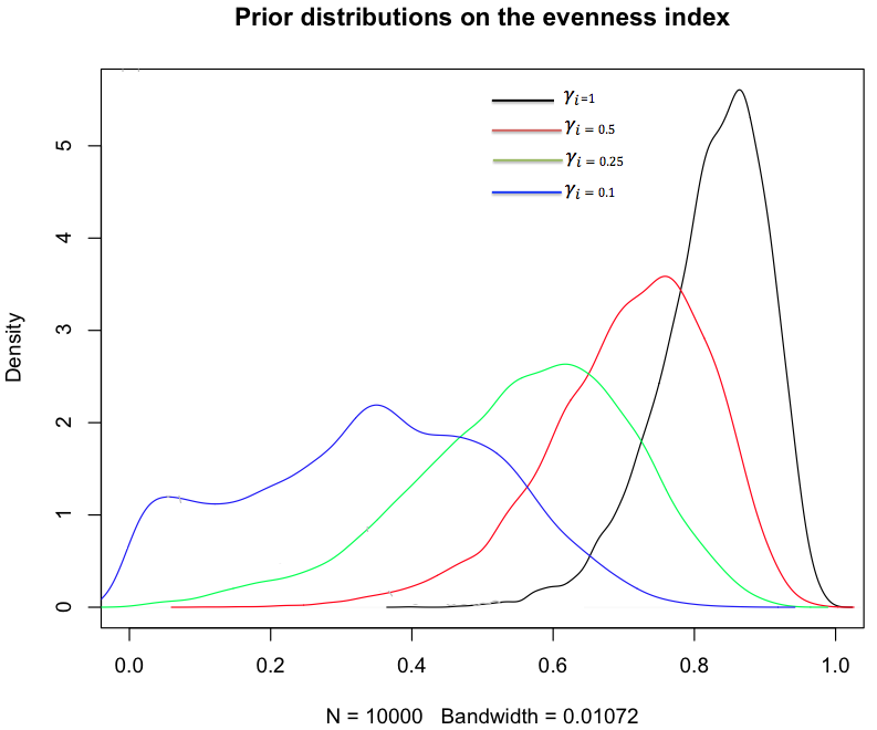
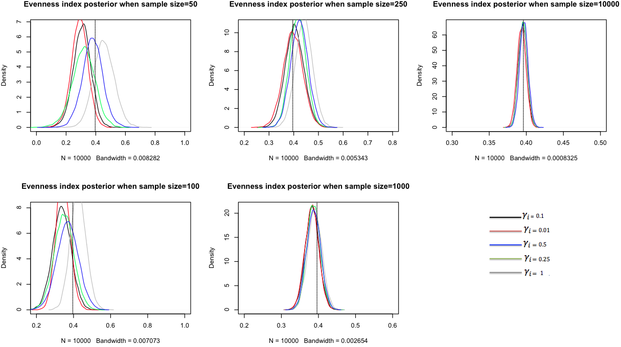
The final example in Seaman III et al (2012) deals with a measure called evenness index $H(\theta)={-\sum\theta_{i}\log(\theta_{i})}\big{/}{\log(K)}$ that is a function of a vector $\theta$ of proportions $\theta_{i}$, $i=1,\ldots,K$. The authors assume a Dirichlet prior on $\theta$ with hyperparameters first equal to $1$ then to $0.25$. For the transform $H(\theta)$, Figure 6 shows that the first prior concentrates on $(0.5,1)$ whereas the second does not. Since there is nothing special about the uniform prior, re-running the evaluation with the Jeffreys prior reduces this feature, which anyway is a characteristic of the prior distribution, not of a posterior distribution that would account for the data. The authors actually propose to use the $\mathrm{Dir}(1/4,1/4,\ldots,1/4)$ prior, presumably on the basis that the induced prior on the evenness is then centered close to 0.5. If we consider the more generic $\mathrm{Dir}(\gamma_{1},\ldots,\gamma_{K})$ prior, we can investigate the impact of the $\gamma_{i}$’s when they move from $0.1$ to $1$. In Figure 6, the induced priors on $H(\theta)$ indeed show a decreasing concentration of the posterior on $(0.5,1)$ as $\gamma_{i}$ decreases towards zero. To further the comparison, we generated datasets of size $N=50,100,250,1000,10,000$. Figure 7 shows the posteriors associated with each of the four Dirichlet priors for these samples, including modes that are all close to $0.4$ when $N=10^{4}$. Even for moderate sample sizes like $50$, the induced posteriors are almost similar. When the sample size is $50$, Table 5 shows there is some degree of variation between the posterior means, even though, as expected, this difference vanishes when the sample size increases.

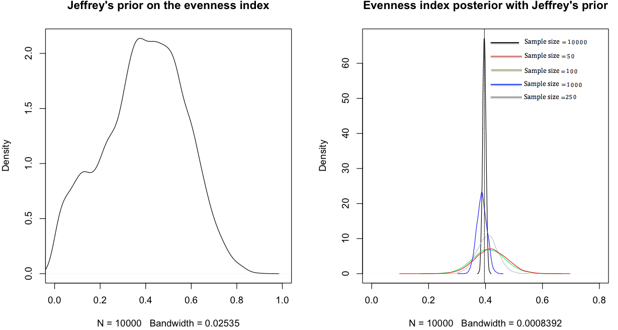
Note that, while Dirichlet distributions are conjugate priors, hence potentially lacking in robustness, Jeffreys’s prior is a special case corresponding to $\gamma_{i}=1/K$ (here $K$ is equal to $8$). Figure 8 reproduces the transform of Jeffreys’ prior for the evenness index (left) and the induced posterior densities for the same values of $N$. Since it is a special case of the above, the same features appear. A potential alternative we did not explore is to set a non-informative prior on the hyperparameters of the Dirichlet distribution.

Figure 6: Priors induced on the evenness index: Four Dirichlet prior are assigned to $\theta$ with hyperparameters all equal to $0.1,0.25,0.5,1$, based on $10^{4}$ simulations.

Figure 7: Estimated posterior densities of $H(\theta)$ considering sample sizes of $50,100,250,1000,10,000$. They correspond to the priors on $\theta$ shown in Figure 6 and are based on $10^{4}$ posterior simulations. The vertical line indicates the mode of all posteriors when sample size is large enough.

Table 5: Posterior means of $H(\theta)$ for the priors shown in Figure 6 and Jeffreys’ prior on $\theta$ for sample sizes $50,100,250,1000,10,000$.

Sample size 50 100 250 1000 10,000 Dirichlet prior when $\gamma_{i}=0.1$ Posterior mean 0.308 0.336 0.403 0.383 0.395 Dirichlet prior when $\gamma_{i}=0.25$ Posterior mean 0.317 0.438 0.417 0.387 0.396 Dirichlet prior when $\gamma_{i}=0.5$ Posterior mean 0.378 0.368 0.423 0.387 0.397 Dirichlet prior when $\gamma_{i}=1$ Posterior mean 0.454 0.425 0.441 0.390 0.396 Jeffreys’ prior: $\gamma_{i}=0.125$ Posterior mean 0.413 0.411 0.406 0.390 0.396 Posterior s.d 0.058 0.057 0.037 0.018 0.006

Figure 8: Jeffreys’ prior and estimated posterior densities of $H(\theta)$ considering sample sizes $50,100,250,1000,10,000$. The posterior distributions are based on $10^{4}$ posterior draws. The vertical line indicates the mode of the posterior density when the sample size is $10^{4}$.

6 Conclusion

In this note, we have reassessed the examples supporting the critical review of Seaman III et al (2012), mostly showing that off-the-shelf noninformative priors are not suffering from the shortcomings pointed out by those authors. Indeed, according to the outcomes produced therein, those noninformative priors result in stable posterior inferences and reasonable Bayesian estimations for the parameters at hand. We thus consider the level of criticism found in the original paper rather unfounded, as it either relies on a highly specific choice of a proper prior distribution or on bypassing basic prior information later used for criticism. The paper of Seaman III et al (2012) concludes with recommendations for prior checks. These recommendations are mostly sensible if mainly expressing the fact that some prior information is almost always available on some quantities of interest. Our sole point of contention is the repeated and recommended reference to MLE, if only because it implies assessing or building the prior from the data. The most specific (if related to the above) recommendation is to use conditional mean priors as exposed by Christensen et al (2011). For instance, in the first (logistic) example, this meant putting a prior on the cdfs at age $40$ and age $60$. The authors picked a uniform in both cases, which sounds inconsistent with the presupposed shape of the probability function.

In conclusion, we find there is nothing pathologically wrong with either the paper of Seaman III et al (2012) or the use of “noninformative” priors! Looking at induced priors on more intuitive transforms of the original parameters is a commendable suggestion, provided some intuition or prior information is already available on those. Using a collection of priors including reference or invariant priors helps as well towards building a feeling about the appropriate choice or range of priors and looking at the dataset induced by simulating from the corresponding predictive cannot hurt.

References

- Barnard et al (2000) Barnard J, McCulloch R, Meng XL (2000) : Modeling Covariance Matrices in Terms of Standard Deviations and Correlations with Application to Shrinkage. Statistica Sinica 10(4):1281–1312
- Berger (1980) Berger JO (1980) : Statistical Decision Theory: Foundations, Concepts, and Methods. Springer-Verl., New York
- Berger (1984) Berger JO (1984) : The Robust Bayesian Viewpoint (with discussion). Robustness of Bayesian Analysis pp 63–144
- Bernardo and Smith (2009) Bernardo JM, Smith AF (2009) : Bayesian Theory. (Vol. 405), John Wiley & Sons, New York
- Box and Tiao (2011) Box GE, Tiao GC (2011) : Bayesian Inference in Statistical Analysis. (Vol. 40), John Wiley & Sons, New York
- Christensen et al (2011) Christensen R, Johnson WO, Branscum AJ, Hanson TE (2011) : Bayesian Ideas and Data Analysis: An Introduction for Scientists and Statisticians. CRC Press, Chapman & Hall
- Cowles (2002) Cowles MK (2002) : Bayesian Estimation of the Proportion of Treatment Effect Captured by Surrogate Marker. Statistics in Medicine 21(6):811–834
- Firth (1993) Firth D (1993) : Bias Reduction of Maximum Likelihood Estimates. Biometrika 80(1):27–38
- Gelman et al (2013) Gelman A, Carlin JB, Stern HS, Dunson DB, Vehtari A, Rubin DB (2013) : Bayesian Data Analysis. CRC press, Chapman & Hall
- Jaynes (2003) Jaynes E (2003) Probability Theory. Cambridge University Press, Cambridge
- Jeffreys (1939) Jeffreys H (1939) Theory of Probability, 1st edn. The Clarendon Press, Oxford
- Laplace (1820) Laplace PS (1820) : Théorie Analytique des Probabilités. Courcier, Paris
- Liang et al (2008) Liang F, Paulo R, Molina G, Clyde MA, Berger JO (2008) : Mixtures of G-priors for Bayesian Variable Selection. The American Statistical Association 103(481):410–423
- Lopes and Tobias (2011) Lopes HF, Tobias JL (2011) : Confronting Prior Convictions: On Issues Prior Sensitivity and Likelihood Robustness Bayesian Analysis. Annu Rev of Economics 3(1):107–131
- Marin and Robert (2007) Marin JM, Robert CP (2007) : Bayesian Core: A Practical Approach to Computational Bayesian Statistics. Springer
- Rissanen (2012) Rissanen J (2012) Optimal Estimation of Parameters. Cambridge University Press
- Robert (2007) Robert CP (2007) : The Bayesian Choice: From Decision-Theoretic Foundations to Computational Implementation. Springer, Springer Science & Business
- Seaman III et al (2012) Seaman III JW, Seaman Jr JW, Stamey JD (2012) : Hidden Dangers of Specifying Noninformative Priors. The American Statistician 66(2):77–84
- Stojanovski and Nur (2011) Stojanovski E, Nur D (2011) : Prior Sensitivity Analysis for a Hierarchical Model. Proceeding of the Fourth Annual ASEARCH Conference pp 64–67
- Welch and Peers (1963) Welch B, Peers H (1963) : On Formulae for Confidence Points based on Integrals of Weighted Likelihoods. Journal of the R Statistical Society Ser B (Methodological) 25:318–329
- Zellner (1986) Zellner A (1986) : On Assessing Prior Distributions and Bayesian Regression Analysis with G-Prior Distributions. In Bayesian Inference and Decis Tech: Essays in Honor of Bruno de Finetti 6:233–243