Small clusters Renormalization Group in 2D and 3D Ising and BEG models with ferro, antiferro and quenched disordered magnetic interactions

Abstract

The Ising and Blume-Emery-Griffiths (BEG) models critical behavior is analyzed in 2D and 3D by means of a renormalization group scheme on small clusters made of a few lattice cells. Different kinds of cells are proposed for both ordered and disordered model cases. In particular, cells preserving a possible antiferromagnetic ordering under renormalization allow for the determination of the Néel critical point and its scaling indices. These also provide more reliable estimates of the Curie fixed point than those obtained using cells preserving only the ferromagnetic ordering. In all studied dimensions, the present procedure does not yield a strong disorder critical point corresponding to the transition to the spin-glass phase. This limitation is thoroughly analyzed and motivated.

I Introduction

In this work we shall discuss the real space Renormalization Group (RG) study of critical behavior of spin systems interacting via different types of magnetic interaction. We will consider the Ising and the Blume-Emery-Griffiths (BEG) models, where spins can take either the value $\pm 1$, magnetic site, or $0$, hole.

The real space RG is based on a number of RG transformations. Different RG transformations have been used in literature, all sharing the property of being “simple”, i.e., the space of allowed couplings must be kept low-dimensional avoiding their proliferation. This process necessarily involves arbitrary and uncontrolled approximations. One possible approach is to replace the original lattice by a different lattice obtained by a bond-moving procedure. This is the case of the hierarchical lattices (see Ref. [Kaufman and Griffiths, 1981; Griffiths and Kaufman, 1982] for the definition and, e.g., Ref. [Salmon et al., 2010] for a recent summary of the achievements). The main drawback is that hierarchical lattices are quite inhomogeneous and have geometrical properties that differ from those of Bravais lattices even locally, sometimes leading to different physical behaviors Antenucci et al. (2014).

In this work, instead, we employ alternative cell blocks transformations, such as those proposed in the seventies, e.g., in Refs. [Niemeijer and Leeuwen, 1973; Berker and Wortis, 1976]. In particular, this approach is proven reliable in the study of the percolation problem Reynolds et al. (1977, 1978), where each site is present with a given probability, independent of the state of the neighbors sites. When site interactions are introduced, this real space RG approach has turned out to be quite powerful for studying the Paramagnetic (PM) – Ferromagnetic (FM) transition, while it often fails to detect more complex phases, such as the antiferromagnetic (AFM) phase in system with antiferromagnetic interactions or the spin-glass (SG) phase in disordered systems.

In this paper we start from the cluster approximation for ferromagnets used by Berker and Wortis Berker and Wortis (1976) and we will consider possible generalizations to more structured block RG transformations to capture the Néel point of antiferromagnetic systems, and we will analyze the robustness of both the FM Curie and AFM Néel critical points to a small amount of disorder. We shall also investigate the possibility of the onset of a SG critical point in the case of strong quenched disorder.

The construction of the block RG transformation is regulated by two opposite requirements: (i) minimal cluster structure to capture the properties of the phases and (ii) computational feasibility. In particular the last request again results in a “hierarchical structure” of the system, different from the original Bravais lattice, such to prevent the development of different kinds of interaction at every RG step. However, in contrast to hierarchical lattices, the local geometry of the Bravais lattice is preserved.

We will consider the critical behavior in both 2D and 3D dimensions, and compare our results to the outcome of numerical simulations and, for small disorder, to the predictions of the gauge theory of Nishimori Nishimori (2001).

The paper is organized as follows. Section II is devoted to 2D Ising models. Here we also recall the real space block RG transformation procedure, and its extension to the case of (quenched) random interactions. We also introduce the generalization of the block RG transformation used to tackle antiferromagnetic and disordered interactions. In Sec. III we extend the analysis to 3D Ising models and in Sec. IV to the Blume-Emery-Griffiths model.

Finally, in Sec. V we summarize our findings and we comment about the inability to locate a SG critical point for strong disorder, and how it might be overcome.

II Cluster Renormalization Group for the 2D Ising model

The real space block RG transformation dates back to the 70’s, and consists of the following steps:

1. group spins on the real space Bravais lattice into blocks with a given geometry;

2. replace each block by a new spin variable, block-spin, whose value is dictated by the values of all the spins inside cell through a projection matrix;

3. sum in the partition over all spins inside the cells for fixed value of the block-spins;

4. rescale the lattice-space to its original value and compute the new, renormalized, values of interactions among the block-spins leaving the partition function invariant.

When points 1 to 4 are iterated they yield the RG flow $\boldsymbol{\mathcal{K}}_{R}=\mathcal{R}(\boldsymbol{\mathcal{K}})$ in the interaction parameters space $\boldsymbol{\mathcal{K}}$. Starting from the initial physical values the renormalized parameters flow towards a fixed point $\boldsymbol{\mathcal{K}}^{*}=\mathcal{R}(\boldsymbol{\mathcal{K}}^{*})$ that characterizes the phase of the system. The stability matrix of the fixed point gives the critical exponents.

In this Section we apply this procedure to the 2D Ising model with quenched disordered bimodal ferromagnetic/antiferromagnetic interactions. The Hamiltonian, expressed in a form suitable for the RG study, is

$$-\beta\mathcal{H}(\bm{s})=\sum_{\langle ij\rangle}\left[J_{ij}s_{i}s_{j}+h_{ij}\frac{s_{i}+s_{j}}{2}+h_{ij}^{\dagger}\frac{s_{i}-s_{j}}{2}\right],$$ (1)

where $\langle ij\rangle$ denotes the ordered sum over nearest-neighbor sites on the 2D Bravais lattice. As usual in RG studies, we use reduced parameters where the temperature is absorbed into the interactions parameters.

The initial (physical) probability distribution of the couplings is

$$P({\mathcal{K}}_{ij})= P(J_{ij})\,P(h_{ij})\,P(h^{\dagger}_{ij})$$

$$= \bigl{[}(1-p)\delta(J_{ij}+J)+p\delta(J_{ij}-J)\bigr{]}$$

$$\phantom{==}\times\delta\bigl{(}h_{ij}-h\bigr{)}\,\delta\bigl{(}h_{ij}^{\dagger}\bigr{)}\,,$$ (2)

where $\boldsymbol{\mathcal{K}}=\{J,h,h^{\dagger}\}$.

II.1 Ferromagnetic 2D Ising model

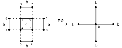
To illustrate, and fix the notation, we shall first discuss the case of the pure ferromagnetic model ($p=1$). Following Berker and Wortis Berker and Wortis (1976) we consider square cells of a 2D square lattice and arrange them in the cluster shown in Fig. 1 (we shall refer to this geometry as “$\text{SQ}_{2}$”). The cluster consists of only two square cells with periodic boundary conditions. The cell $a$ contains spins $\{s_{1},\,s_{2},\,s_{3},\,s_{4}\}$ and the cell $b$ spins $\{s_{5},\,s_{6},\,s_{7},\,s_{8}\}$. This geometry ensures that the block RG transformation does not introduce additional couplings, besides $J$, $h$ and $h^{\dagger}$. Moreover, periodic boundary conditions guarantees that each spin has exactly four neighboring sites, so that the system has the correct multiplicity factor for the completely aligned configurations. A correct multiplicity is a necessary, but not sufficient, requirement for a correct estimation of the critical temperature.

Figure 1: $\text{SQ}_{2}$ cluster [Berker and Wortis, 1976]: two square cells $C=a,\,b$ are arranged with periodic boundary conditions. Full line denotes intra-cell bonds, while dotted lines inter-cell bonds. Under the block RG transformation the cells are replaced by the block-spins $\sigma_{a,b}$. The periodic boundary conditions ensures that each block-spin is connected to the other one by four bonds.

Next for each cell $c$ a new block-spin $\sigma_{c}$ is defined, step 2, using a projection matrix $\mathcal{M}(\sigma_{c},s_{i\in c})$ that maps each configuration of the spin of the cell $s_{i\in c}$ to the value of the block-spin $\sigma_{c}$. The most general projection matrix that preserves the up-down symmetry of the Ising spins is

$$\mathcal{M}(1,s_{i\in c})$$    

with $\mathcal{M}(-1,-s_{i\in c})=\mathcal{M}(1,s_{i\in c})$. The parameter $t$ is a free parameter that controls the relative weight of non-symmetric configurations, and its value can be tuned to fine adjust the outcome of the RG analysis to known results. From its definition one may expect $0\leq t\leq 1$, however we will see that fine tuning may lead to $t$ outside these boundaries. For $t=0$ one recovers the majority rule: the value of the block-spin is the value of the majority of spins of the cell, and $\pm 1$ with equal probability in case of parity. We will refer to the version of the method in which $t$ is different from zero (fixed to correctly obtain known critical points of the model) as tuned two square cells lattice (“$\text{tSQ}_{2}$”).

The next step is done by summing in the partition sum over all possible configurations of the spins of the cells $s_{i}$ for fixed block-spins $\sigma_{c}$. This leads to the renormalized Hamiltonian ${\cal{H}}^{\prime}(\bm{\sigma})$

$$e^{-\beta{\cal{H}}^{\prime}(\bm{\sigma})} =\sum_{\bm{s}}\left[\prod_{c}\mathcal{M}(\sigma_{c},s_{i\in c})\right]e^{-\beta{\cal{H}}(\bm{s})}.$$ (3)

for the block-spin.

The procedure must leave the partition function invariant. Therefore, the final step is the replacement $\sigma\to s$ and a rescaling that changes ${\cal{H}}^{\prime}$ back to the original form of the Hamiltonian in the new spin $s$:

$$-\beta{\cal{H}}_{R}(\bm{s})=\alpha\Bigl{(}J_{R}\,s_{a}s_{b}+ h_{R}\frac{s_{a}+s_{b}}{2}+h^{\dagger}_{R}\frac{s_{a}-s_{b}}{2}\Bigr{)}\,,$$ (4)

with the renormalized interactions:

$$J_{R} =\frac{1}{4\alpha}\log\biggl{(}\frac{x_{++}x_{--}}{x_{+-}x_{-+}}\biggl{)},$$

$$h_{R} =\frac{1}{2\alpha}\log\biggl{(}\frac{x_{++}}{x_{--}}\biggl{)},$$ (5)

$$h^{\dagger}_{R} =\frac{1}{2\alpha}\log\biggl{(}\frac{x_{+-}}{x_{-+}}\biggl{)},$$

where

$$x_{\sigma_{a}\sigma_{b}}=\sum_{\bm{s}}\mathcal{M}(\sigma_{a},s_{i\in a})\,\mathcal{M}(\sigma_{b},s_{i\in b})\,e^{-\beta{\cal{H}}(\bm{s})}\,$$ (6)

are the so-called edge Boltzmann factors. The coefficient $\alpha$ is the number of near-neighbor sites on the lattice, $4$ for the 2D case.

Note that if $h=0$, then $\mathcal{H}(\bm{s})=\mathcal{H}(-\bm{s})$, implying $x_{+-}=x_{-+}$ and $x_{++}=x_{--}$ and, eventually, $h_{R}=h^{\dagger}_{R}=0$.

Equations (II.1)-(6) define the the RG flow $\boldsymbol{\mathcal{K}}_{R}=\mathcal{R}(\boldsymbol{\mathcal{K}})$. The critical exponents are obtained from the eigenvalues of the stability matrix $\partial\boldsymbol{\mathcal{K}}_{R}/\partial\boldsymbol{\mathcal{K}}$ evaluated at the fixed point $\boldsymbol{\mathcal{K}}^{*}$, which can be written in terms of

$$\frac{\partial x_{s_{a}s_{b}}}{\partial J} =\sum_{\overset{\bm{s}}{\langle ij\rangle}}\mathcal{M}(\sigma_{a},s_{i\in a})\,\mathcal{M}(\sigma_{b},s_{i\in b})\,s_{i}s_{j}\,e^{-\beta\mathcal{H}(\bm{s})}\,,$$

$$\frac{\partial x_{s_{a}s_{b}}}{\partial h} =\sum_{\overset{\bm{s}}{\langle ij\rangle}}\mathcal{M}(\sigma_{a},s_{i\in a})\,\mathcal{M}(\sigma_{b},s_{i\in b})\,\frac{s_{i}+s_{j}}{2}\,e^{-\beta\mathcal{H}(\bm{s})}\,,$$

$$\frac{\partial x_{s_{a}s_{b}}}{\partial h^{\dagger}} =\sum_{\overset{\bm{s}}{\langle ij\rangle}}\mathcal{M}(\sigma_{a},s_{i\in a})\,\mathcal{M}(\sigma_{b},s_{i\in b})\,\frac{s_{i}-s_{j}}{2}\,e^{-\beta\mathcal{H}(\bm{s})}.$$

The nontrivial fixed point(s) are for $h=h^{\dagger}=0$. In this case the stability matrix is diagonal and the relevant scaling exponent are $y_{T}=\log_{b}(\partial/\partial_{J})J_{R}$ and $y_{h}=\log_{b}(\partial/\partial_{h})h_{R}$, where $b$ is the lattice scaling factor, equal to $2$ for the $\text{SQ}_{2}$ cluster of Fig. 1. The critical exponents are then

$$\nu =\frac{1}{y_{T}}\,, \eta =d+2-2y_{h}.$$ (7)

The others follow from the scaling laws.

The numerical implementation of this procedure gives for the ordered ferromagnetic 2D Ising model ($p=1$) the critical temperature $T_{\text{c}}=J_{c}^{-1}=1.896$ for the PM/FM transition, and scaling exponents $y_{T}=0.727$ and $y_{h}=1.942$, see also Ref. [Berker and Wortis, 1976]. The value $y_{h}$ is less than the dimension of the space, implying that the transition is of the second order Nienhuis and Nauenberg (1975). The values of the critical exponents are shown in the first row of Table 1.

By comparing with the exact Onsager solution Onsager (1943), the critical temperature deviates of about $20\%$ from the exact result $T_{\text{c}}^{\rm Ons}=2/\log(1+\sqrt{2})=2.2692...$ and the values of the critical exponent all suffer major deviations. We postpone the discussion on how this estimates could be improved.

	$\boldsymbol{\alpha}$	$\boldsymbol{\beta}$	$\boldsymbol{\gamma}$	$\boldsymbol{\delta}$	$\boldsymbol{\nu}$	$\boldsymbol{\eta}$
$\text{SQ}_{2}$	-0.7523	0.08038	2.592	33.24	1.376	0.1168
$\text{tSQ}_{2}$ Ons.	-0.1233	0.1383	1.847	14.35	1.062	0.2606
$\text{tSQ}_{2}$ Nish.	-1.426	0.05884	3.309	57.23	1.713	0.06870
$\text{SSQ}_{2}$	-0.6545	0.2141	2.226	11.40	1.327	0.3226
$\text{SQ}_{4}$	-0.1524	0.1915	1.769	10.24	1.076	0.3559
$\text{SSQ}_{4}$	-0.4458	0.4779	1.490	4.118	1.222	0.7815
Exact	0	0.125	1.75	15	1	0.25

Table 1: Critical exponents of the ferromagnetic 2D Ising Model obtained with the different clusters discussed in this work compared with the known exact results. In the second (third) line the parameter $t$ is fixed to reproduce the known Onsager (Nishimori) critical temperature of the 2D lattice.

II.2 Disordered 2D Ising Model

In presence of quenched disorder the RG flow cannot be restricted to single interaction values $\boldsymbol{\mathcal{K}}$, and necessarily involves the whole coupling probability distribution $P(\boldsymbol{\mathcal{K}})$. The RG equation then becomes

$$P_{R}(\boldsymbol{\mathcal{K}}_{R})=\int d\boldsymbol{\mathcal{K}}\,P(\boldsymbol{\mathcal{K}})\,\delta\bigl{[}\boldsymbol{\mathcal{K}}_{R}-{\cal R}(\boldsymbol{\mathcal{K}})\bigr{]}.$$ (8)

The block RG transformation must then be repeated starting from interaction parameters configurations $\boldsymbol{\mathcal{K}}$ extracted with probability $P(\boldsymbol{\mathcal{K}})$. The outcomes $\boldsymbol{\mathcal{K}}_{R}$ are then used to construct the renormalized probability distribution $P_{R}(\boldsymbol{\mathcal{K}})$, which, in turn, is used as entry for the next iteration.

In a numerical study, the number of possible interaction parameter configurations that can be considered is finite. The flow of the renormalized probability distribution $P_{R}(\boldsymbol{\mathcal{K}})$ can then be followed by using a method initially suggested in Ref. [Southern and Young, 1977]. One first sets up a starting pool of $M\gg 1$ different randomly chosen real numbers produced according to the initial probability of the couplings, Eq. (2) for the bimodal Ising Model. Then a coupling configuration $\boldsymbol{\mathcal{K}}$ is constructed by randomly picking numbers from the pool and assigning them to the couplings. A renormalized $\boldsymbol{\mathcal{K}}_{R}$ is, thus, evaluated. The procedure is repeated $M$ times obtaining a new pool that represents the renormalized probability distribution, from which one can compute the moments and estimate $P_{R}(\boldsymbol{\mathcal{K}})$ from the frequency histogram.

In Fig. 2 we show the flow of the probability distribution $P(J_{ij})$ of a single pool in the disordered 2D Ising model (1)-(2) with $h=0$ and $p=0.9$ generated by the block RG transformation on the $\text{SQ}_{2}$ cluster. In the upper figure, $\,T=J^{-1}=1.4$, the average $\mu_{J}$ moves towards smaller values while the width of the distribution shrinks. This signals a PM phase, with the PM fixed point probability distribution function of mean $\mu_{J}\to 0$ and variance $\sigma_{J}^{2}\to 0$. In the lower figure, $T=J^{-1}=1.2$, the probability distribution width narrows while shifting towards larger value of $\mu_{J}$. This denotes a FM phase, with the FM fixed point probability specified by $\mu_{J}\to\infty$ and $\sigma_{J}/\mu_{J}\to 0$. We observe that a SG phase would be signaled by a fixed point probability distribution with $\sigma_{J}\to\infty$ while $\mu_{J}/\sigma_{J}\to 0$, so that spins at great distance are still strong interacting but the sign of the interaction is not defined.

Figure 2: RG flow of the probability distribution $P(J_{ij})$ for the disordered 2D Ising model (1)-(2) with $h=0$ and $p=0.9$. obtained with the $\text{SQ}_{2}$ cluster. The histograms are obtained by taking $5\cdot 10^{3}$ bins around the mean value $\mu_{J}$. The bin width is fixed by the requirement that $99.9\%$ of the values are inside the grid used to follow the histogram flow. Upper Figure: $T=J^{-1}=1.4$, evidence for PM phase. Lower Figure: $T=J^{-1}=1.2$, $p=0.9$, evidence for FM phase.

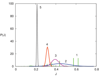
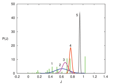
To reduce the possible bias introduced by the choice of the initial pool, Nobre et al. Nobre (2001) have proposed to repeat the block RG transformations using a set of $N_{s}$ samples with different initial pools of size $M$. When close to a critical point flows originating from different pools may flow towards different fixed point distributions. The size of the region where the phase is not uniquely identified gives the uncertainty on the critical value obtained with a the pools of size $M$.

In our numerical study of the disordered 2D Ising model we have used $N_{s}=20$ pools of size $M=10^{6}$ each, and we have assumed a phase uniquely defined if at least $80\%$ of the RG flows flow towards the same fixed distribution. With this choice the uncertainty is generally less than $0.1\%$ and the systematic error considerably decreased.

Figure 3: ($p,T)$ phase diagram of the disordered 2D Ising model obtained with the $\text{tSQ}_{2}$ cluster and different choices for the parameter $t$ in the projection matrix. Filled square: $t=0$; Empty circle: $t=-0.06453$ fixed by the requirement $T_{\text{c}}(p=1)=T_{\text{c}}^{\rm Ons}$ (Onsager); Empty square: $t=0.0304$ fixed by the requirement $T_{\text{c}}(p_{\text{mc}})=T_{\text{mc}}$ (Nishimori); Dashed line: Nishimori line.

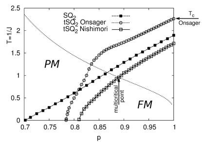
The $(p,T)$ phase diagram of the disordered 2D Ising model obtained using the $\text{SQ}_{2}$ cluster is shown in Fig. 3 (black squares). As the probability $p$ of the ferromagnetic bonds is lowered the critical temperature decreases until, for low enough $p$, the FM phase disappears. In the figure also the Nishimori line Nishimori (1981)

$$\frac{1}{T}=\frac{1}{2}\log\frac{p}{1-p}$$ (9)

is shown. Along this line the model is invariant under the gauge transformation of spins and interactions and exact information about the phase diagram can be obtained Nishimori (2001). The point where the Nishimori line crosses the transition line is called “multicritical”: when a SG phase is actually present, this is the point at which PM, FM and SG phases all are in contact with each other.

By the RG on the $\text{SQ}_{2}$ cluster the “multicritical” point is found at $p_{\text{mc}}=0.8667$, $T_{\text{mc}}=1.070$. For $p<p_{\text{mc}}$, exact results impose no FM ordering Nishimori (2001). Inspection of the Figure shows that not only the method fails to predict the correct critical temperature $T_{\text{c}}^{\rm Ons}$ of the pure ferromagnetic model, but also the requirements following from the gauge theory.

One can try to improve the numerical estimates tuning the parameter $t$ in the projection matrix to fix some known points in the $(p,T)$ diagram. We consider two possible choices: fixing the critical temperature of the pure system to the exact value or the crossing point with the Nishimori line to the multicritical point. The requirement $T_{\text{c}}=T_{\text{c}}^{\rm Ons}$ leads to $t=-0.06453$, while the requirement $T_{\text{c}}(p_{\text{mc}})=T_{\text{mc}}$ to $t=0.0304$. Note the “unphysical” negative value of $t$, also used by Berker and Wortis Berker and Wortis (1976), which implies that under the block transformation the contribution of some spin configurations of the cell to the partition sum can be negative. The transition lines obtained with these choices for $t$ are shown in Fig. 3. In both cases, and besides the unphysical values of $t$, the slope of the transition line increase as $p$ decreases, but still no re-entrance or vertical line is recovered. In either cases the only critical point remains the FM fixed point at $p=1$ with scaling exponents $y_{T}=0.9419$ and $y_{h}=1.870$ for $t=-0.06453$, and $y_{T}=0.5837$ and $y_{h}=1.965$ for $t=0.0304$. The numerical values of the critical exponents are shown in the second and third row of Table 1, respectively. Note that in all cases $\alpha<0$. According to the Harris criterion Harris (1974) this indicates that the FM fixed point is stable against the introduction of a small amount of quenched disorder.

Summarizing the results: the block RG transformation based on the $\text{SQ}_{2}$ cluster finds no true multicritical point, nor a “strong disorder” fixed point, and, hence, no change in the universality class of the critical behavior is detected.

II.3 Antiferromagnetic order: need for “$\text{SSQ}_{2}$”

Another important issue of the block RG transformation discussed so far is the absence of an AFM phase. Below some critical value of $p$ and down to $p=0$, only the PM phase is found. This failure might also strongly bias the quest for a spin-glass phase in dimension higher than two.

By analyzing the block RG transformation used so far, we see that it assigns the same weight to symmetric configurations (e.g., $++--$) of the spins of the cell, regardless of their ordering. As a consequence, it is not able to identify an antiferromagnetic ordering, and a staggered magnetization cannot be properly defined.

We thus need a cluster construction that distinguishes the symmetry breaking ordering associated with the AFM phase. By referring to labeling of Fig. 1, we then assign the spins $\{s_{1},s_{3},s_{5},s_{7}\}$ to the cell $a$ and the spins $\{s_{2},s_{4},s_{6},s_{8}\}$ to the cell $b$, shaping a staggered topology (“$\text{SSQ}_{2}$” in the following). The projection matrix of the cell remains unchanged. The phase diagram obtained through this block RG transformation is shown in Fig. 4. The improvement with respect to the $\text{SQ}_{2}$ cluster is evident. The $p=0$ antiferromagnetic critical point is now found, as well as a PM/AFM transition line for $p>0$. Since in this model, for $h=0$ the symmetry $(p,J)\leftrightarrow(1-p,-J)$ holds and the staggered cluster preserves AFM ordering, the PM/AFM line is symmetric to the PM/FM line with respect to $p=1/2$. The behavior of the critical line below $p_{\text{mc}}$, however, still violates the requirement imposed by the gauge theory.

Figure 4: $T$, $p$ phase diagram of the Ising 2D model as obtained by iterating the RG on different clusters with two and four cells. The dashed line is Nishimori line, Eq. 9.

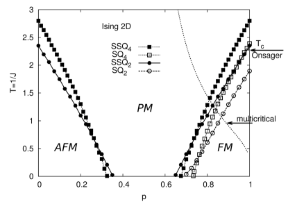
The $\text{SSQ}_{2}$ cluster improves the estimate of the pure critical fixed point ($p=1$). The critical temperature turns out $T_{\text{c}}(p=1)=2.352$ and deviates of about $3.5\%$ from Onsager result. The scaling exponents are $y_{T}=0.7534$ and $y_{h}=1.839$, and the associated critical exponents are reported in Table 1. Though they display differences of $20\%$ to $40\%$ from the exact values, their estimates are sensitively better than those obtained with the classic $\text{SQ}_{2}$ cluster.

As the AFM transition is concerned, the behavior is specular to that of the FM transition. The points along the AFM critical line are attracted by a unique second order AFM Néel fixed point at $p=0$ at the same critical temperature $T_{\text{c}}(p=0)=2.352$ with scaling exponents $y_{T}=0.7534$, as found for the FM fixed point, and $y_{h}=0.01565$. The symmetry of the RG equations implies that the PM/AFM and PM/FM fixed points have the same $y_{T}$. The values of $y_{h}$ are, however, quite different, the AFM one being almost zero. The reason is that the magnetization is not the correct order parameter for the AFM transition, as it remains zero on both sides of the transition. If, rather, the staggered magnetization is considered, and, hence, a staggered field $h^{\dagger}$ is introduced in the Hamiltonian, then the relevant scaling exponent turns out to be $y_{h^{\dagger}}=\log_{2}\partial_{h^{\dagger}}h^{\dagger}_{R}=1.797\gg y_{h}$.

II.4 $4$-square cells cluster (“$\text{SQ}_{4}$”)

The $\text{SSQ}_{2}$ cluster leads to an AFM fixed point, and improves both the analysis of the AFM and FM phases. However, it does not allow for possible frustrated configurations in the renormalized cells. In an attempt to circumvent this problem we extend the cluster from two to four cells.

Figure 5: The $16$-spins $\text{SQ}_{4}$ cluster: before (lhs.) and after (rhs.) renormalization. Full lines denote intra-cell bonds, while dotted lines inter-cell bonds due to periodic boundary conditions. Block-spins $\sigma_{a,b,c,d}$ on the rhs. cluster are constructed from spins $s_{i=1,\ldots,16}$ denoted by the same symbol on the lhs. cluster.

As the number of cells increases, so does the number of possible cluster definitions. We found that the best block RG transformation, in terms of similarity with the exact results, is obtained with the cluster shown in Fig. 5. The block RG transformation is performed by summing in the partition sum over all possible configurations of the spins of the cells $s_{i=1,\ldots,16}$ for fixed block-spins

$$\sigma_{a} :=\{s_{1},s_{2},s_{3},s_{4}\}\,,$$

$$\sigma_{b} :=\{s_{5},s_{6},s_{7},s_{8}\}\,,$$

$$\sigma_{c} :=\{s_{9},s_{10},s_{11},s_{12}\}\,,$$

$$\sigma_{d} :=\{s_{13},s_{14},s_{15},s_{16}\}\,.$$

The $16$ spins of the SQ₄ cluster, together with the inter-cell interactions from periodic boundary conditions, form a $4\times 4$ array of $4$-spin cells. The block RG transformation generates, besides nearest-neighbor interactions, also next-nearest-neighbor interactions and “plaquette” interactions.

To avoid truncations we, then, start from the more general Hamiltonian

$$-\beta\mathcal{H}(\bm{s})= \frac{1}{2}\sum_{{\bm{i}}}\sum_{k=1}^{4}J_{{\bm{i}},{\bm{i}+\boldsymbol{\mu}_{k}}}s_{\bm{i}}s_{\bm{i}+\boldsymbol{\mu}_{k}}\,+$$

$$+\frac{1}{2}\sum_{{\bm{i}}}\sum_{k=1}^{4}K_{\bm{i},{\bm{i}+\boldsymbol{\eta}_{k}}}s_{\bm{i}}s_{\bm{i}+\boldsymbol{\eta}_{k}}\,+$$ (10)

$$+\sum_{{\bm{i}}}D_{\bm{i}}\prod_{k=1}^{4}s_{\bm{i}+\boldsymbol{\xi}_{k}}\,,$$

where ${\bm{i}}=(i_{x},i_{y})$ denotes a site on the 2D lattice, $\boldsymbol{\mu}$ the relative position of the nearest-neighbor sites, $\boldsymbol{\eta}$ the relative position of the next nearest-neighbor sites and $\boldsymbol{\xi}$ the relative position of the plaquette sites:

$\boldsymbol{\mu}_{1}=(0,1)\,,$	$\boldsymbol{\mu}_{2}=(1,0)\,,$	$\boldsymbol{\mu}_{3}=(0,-1)\,,$	$\boldsymbol{\mu}_{4}=(-1,0)\,,$
$\boldsymbol{\eta}_{1}=(1,1)\,,$	$\boldsymbol{\eta}_{2}=(1,-1)\,,$	$\boldsymbol{\eta}_{3}=(-1,-1)\,,$	$\boldsymbol{\eta}_{4}=(-1,1)\,,$
$\boldsymbol{\xi}_{1}=(0,0)\,,$	$\boldsymbol{\xi}_{2}=(0,1)\,,$	$\boldsymbol{\xi}_{3}=(1,1)\,,$	$\boldsymbol{\xi}_{4}=(1,0).$

The initial distributions of the couplings is

$$P(\boldsymbol{\mathcal{K}}_{ij})\!\!=\!\left[(1\!-p)\delta(J_{ij}+\!J)+p\delta(J_{ij}-\!J)\right]\delta\!\left(K_{ij}\right)\delta\!\left(D_{i}\right)\,.$$

Figure 6: Allocation of the interactions for the SQ₄ cluster. The interactions $J,$ $K,$ $D$ are represented respectively by horizontal and vertical lines, diagonal lines, and circles. Ensembles of adjacent 2$J$s, 2$K$s and 1 $D$ are grouped together to form “arrow packages” that completely cover both the initial and the renormalized clusters of Fig. 5. These ensembles are the building blocks of the RG procedure, so that the correlation between the interactions in the ensembles is preserved under the renormalization.

To best preserve the correlation between the interactions $J$, $K$ and $D$ we build the pools that numerically represent the interaction probability distribution by correlated ensembles consisting of 2 $J$s, 2 $K$s and 1 $D$ adjacent to each other. These are the maximum sets that completely cover both the initial and the renormalized clusters, as shown in Fig. 6. Notice that, because of the periodic boundary conditions, the four ensembles in the renormalized system of Fig. 6 only differ in the values for the $J$s, while the $K$s and the $D$ are always the same.

The block RG with the Hamiltonian (II.4) leads to four $J$-like ($J_{R}^{\pm},\,\tilde{J}_{R}^{\pm}$), two $K$-like ($K_{R}^{\pm}$) and one $D$-like ($D_{R}$) renormalized interactions whose values are

$$J_{R}^{\pm} =\frac{1}{16}\left(\log\frac{x_{++++}\,x_{--++}}{x_{+-+-}\,x_{+--+}}\pm\log\frac{x_{++-+}\,x_{+++-}}{x_{+-++}\,x_{-+++}}\right)$$

$$\tilde{J}_{R}^{\pm} =\frac{1}{16}\left(\log\frac{x_{++++}\,x_{+--+}}{x_{+-+-}\,x_{--++}}\pm\log\frac{x_{-+++}\,x_{+++-}}{x_{++-+}\,x_{+-++}}\right)$$

$$K_{R}^{\pm} =\frac{1}{32}\left(\log\frac{x_{++++}\,x_{+-+-}}{x_{--++}\,x_{+--+}}\pm\log\frac{x_{+-++}\,x_{+++-}}{x_{++-+}\,x_{-+++}}\right)$$

$$D_{R} =\frac{1}{32}\log\frac{x_{++++}\,x_{+-+-}\,x_{--++}\,x_{+--+}}{x_{+-++}\,x_{+++-}\,x_{++-+}\,x_{-+++}},$$ (11)

with the edge Boltzmann factors

$$x_{\sigma_{a}\sigma_{b}\sigma_{c}\sigma_{d}}=\sum_{\bm{s}} \mathcal{M}_{a}\mathcal{M}_{b}\mathcal{M}_{c}\mathcal{M}_{d}\,e^{-\beta{\cal{H}}(\bm{s})},$$

where $\mathcal{M}_{x}\equiv\mathcal{M}(\sigma_{x},s_{i\in x})$ are the cell projection matrices. The renormalized $J$s are assigned to the the 4 renormalized ensembles as $\{J_{R}^{+},\,\tilde{J}_{R}^{-}\}$, $\{\tilde{J}_{R}^{-},\,\tilde{J}_{R}^{+}\}$, $\{\tilde{J}_{R}^{+},\,J_{R}^{-}\}$, $\{J_{R}^{-},\,J_{R}^{+}\}$.

The phase diagram obtained with $N_{s}=10$ pools of size $M=10^{6}$ is shown in Fig. 4, line $\text{SQ}_{4}$. All the points on the critical line are attracted by the pure fixed point at $p=1$ and critical temperature of $T_{\text{c}}(p=1)=2.391$, about $5\%$ off the exact 2D result.

To evaluate the critical exponents we have to include in the Hamiltonian an external magnetic field, and hence consider also the three spin interaction $\sum_{\bm{i}}\sum_{k=1}^{4}s_{\mathbf{i}}\,s_{\mathbf{i}+\boldsymbol{\mu}_{k}}\,s_{\mathbf{i}+\boldsymbol{\mu}_{k+1}}$ generated by the RG. This gives a total of five parameters. At the pure fixed point only two are relevant with scaling exponent $y_{T}=0.9292$ and $y_{h}=1.822$. The values of the associated critical exponents are reported in the fifth line of Table 1

The re-entrance of the critical line below the multicritical point $T_{\text{c}}(p)<T_{\text{mc}}$ is still absent. However, the line appears steeper than those obtained with the previous block RG transformations, approaching the expected behavior of the model. Despite this qualitative improvement, the intersection between the transition line and the Nishimori line occurs sensitively above the exact multicritical point, cfr. Table 2, and, as in the previous cases, it does not correspond to a real multicritical point..

The RG analysis indeed does not show critical fixed points besides the pure critical point at $p=1$. The so called strong disorder fixed point Toldin et al. (2009) is missing and the crossing is not associated with flows towards the FM and strong disorder fixed points.

	T${}_{\text{Ons}}$	p${}_{\text{mc}}$	T${}_{\text{mc}}$
$\text{SQ}_{2}$	1.896	$0.867$	$1.070$
$\text{tSQ}_{2}$ Ons.	2.269	$0.834$	$1.242$
$\text{tSQ}_{2}$ Nish.	1.714	$0.89081$	$0.9528$
$\text{SSQ}_{2}$	2.352	$0.827$	$1.277$
$\text{SQ}_{4}$	2.391	$0.835$	$1.231$
$\text{SSQ}_{4}$	2.802	$0.809$	$1.388$
2D Onsager (1943); Hasenbusch et al. (2008); Ohzeki (2009)	$2.269...$	$0.89081(7)$	$0.9528(4)$

Table 2: Estimate of the FM critical point ($p=1$) temperature ($T_{\text{Ons}}$) and the coordinate of intersection point between the PM/FM transition line with the Nishimori line ($p_{\text{mc}}$, $T_{\text{mc}}$) for the disordered bimodal 2D Ising model obtained with the different block RG transformations discussed in this work, compared with the locations known for the 2D lattice.

II.5 $4$-staggered cells cluster (“$\text{SSQ}_{4}$”)

As found for the $\text{SQ}_{2}$ cluster, the $\text{SQ}_{4}$ cluster does not show an AFM fixed point and the PM/AFM transition is missing. To recover it we then consider the generalization to a staggered grouping of spins for the four cells cluster (“$\text{SSQ}_{4}$”). By referring to the numbering of Fig. 5 :

$$\{s_{1},s_{5},s_{9},s_{13}\} \rightarrow s_{a}\,,$$

$$\{s_{2},s_{6},s_{10},s_{14}\} \rightarrow s_{b}\,,$$

$$\{s_{3},s_{7},s_{11},s_{15}\} \rightarrow s_{c}\,,$$

$$\{s_{4},s_{8},s_{12},s_{16}\} \rightarrow s_{d}\,.$$

The phase diagram obtained with this block RG transformation is shown in Fig. 4. Though we can now identify the PM/AFM transition, we observe a worsening of the estimates of the critical points: $T_{\text{c}}=2.802$ for both the Curie and the Néel points. The points along the PM/FM transition line flow towards the FM fixed point at $p=1$, while those on the PM/AFM transition line are attracted by the AFM fixed point at $p=0$. Therefore also in this case we do not find a strong disorder fixed point.

The two relevant scaling exponents of the stability matrices at the FM critical fixed point are $y_{T}=0.8177$ and $y_{h}=1.609$; see Table 1 for the corresponding critical exponents.

For the AFM fixed point we have $y_{T}=0.8177$, the same of the FM fixed point. As discussed previously, for the AFM transition the relevant order parameter is the staggered magnetization, and the scaling exponent of the staggered field is $y_{h^{\dagger}}=1.569$.

To summarize, for the 2D Ising model with bimodal disorder, Eq. (2), we have evidence for both PM/FM and PM/AFM transition for large enough $|p|$. Quantitatively, the best estimates for the Curie and Néel critical points are obtained in the $\text{SSQ}_{2}$ cluster scheme (cfr. Table 2). The multi critical point is missing since we do not find any strong disorder fixed point. No SG phase can be tested because we are in dimension $d<2.5$. Therefore in the next Section we move to the 3D case.

III Cluster Renormalization Group for the 3D Ising model

In this Section we extend the method based on the $\text{SQ}_{2}$ cluster to the three dimensional case, by using the cluster of two cubic cells with periodic boundary conditions shown in Fig. 7 (referred as “$\text{CB}_{2}$”) for the study of the 3D Ising model.

Figure 7: Three dimensional two cells cluster. With the cell grouping in figure (solid lines) we refer to it as “CB₂”.

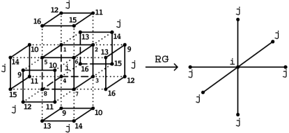
The associated projection matrix is

$$\quad\mathcal{M}(1,s_{i\in c})\quad$$

and $\mathcal{M}(-1,-s_{i\in c})=\mathcal{M}(1,s_{i\in c})$, which, for $t_{i}=0$, reduces to the majority rule.

The initial probability distribution of the interactions is given in Eq. (2), and we used $N_{s}=10$ pools of size $M=10^{6}$. The phase diagram for $\text{CB}_{2}$ cluster is shown in Fig. 8. Once again, only the pure fixed point at $p=1$ controlling the PM/FM transition is found.

Figure 8: Phase diagram in the $(p,T)$ plane of the $\pm J$ 3D Ising model obtained with the block RG transformation using the two cells clusters CB₂ and tCB₂ (see text). The dashed line is the Nishimori line. The $t\not=0$ curve is obtained by fixing the values $t_{i}$ by the requirement $T_{\text{c}}(p=1)=4.5115$.

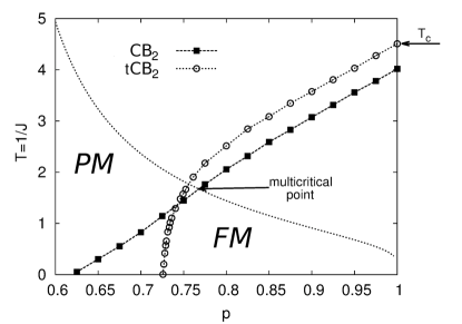
For the choice $t_{i}=0$ the critical temperature is $T_{\text{c}}=4.0177$, which compared with the estimation from numerical simulations $T_{\text{c}}=4.5115$ Talapov and Blöte (1996), has a difference of about $12\%$. The scaling exponents of the fixed point are $y_{T}=1.253$ and $y_{h}=2.684$, the value of the critical exponents are reported in Table 3.

	$\boldsymbol{\alpha}$	$\boldsymbol{\beta}$	$\boldsymbol{\gamma}$	$\boldsymbol{\delta}$	$\boldsymbol{\nu}$	$\boldsymbol{\eta}$
CB2	-0.3952	0.2521	1.891	8.499	0.7984	-0.3684
tCB2	-0.3015	0.4413	1.419	4.215	0.7672	0.1505
SCB2	-0.8887	0.4944	1.900	4.843	0.9629	0.02693
3D Pelissetto and Vicari (2002)	0.1101	0.3265	1.2373	4.789	0.6301	0.03645

Table 3: FM critical exponents of the 3D Ising model obtained with the block RG transformation using the two cells clusters discussed in the text. For the tCB₂ method the values of $t_{i}$ are fixed by the requirement $T_{\text{c}}(p=1)=4.5115$.

The PM/FM transition line crosses the Nishimori line at the point $p_{\text{mc}}=0.76793$ and $T_{\text{mc}}=1.6721$, compatible with the multicritical point obtained for the 3D Ising model on a the cubic lattice Ozeki and Ito (1998): $p_{\text{mc}}=0.7673(4)$, $T_{\text{mc}}=1.676(3)$. Despite this agreement the transition line, however, does not show any re-entrance.

When the parameters $t_{i}$ are fixed by the condition $T_{\text{c}}(p=1)=4.5115$ Talapov and Blöte (1996), leading to $t_{2}=0.011$, $t_{4}=-0.010$ and $t_{6}=-0.050$, the transition line shows a sharp increase of the slope for $p<p_{\text{mc}}$, yet no re-entrance nor vertical part are observed, see tCB₂ line in Fig. 8. There is still only the critical point at $p=1$ and the crossing with the Nishimori line does not correspond to a real multicritical point. The scaling exponent are $y_{T}=1.303$ and $y_{h}=2.425$, and one observes a slight improvement of the values of the critical exponents, see Table 3.

The condition $T_{\text{c}}(p_{\text{mc}})=T_{\text{mc}}$ is compatible with $t_{i}=0$ and does not give new results.

The 3D Ising model is known to present a multicritical point where PM, FM and SG phase meet Nishimori (1981). Contrarily to numerical simulation predictions, where $\alpha=2-d\nu>0$ Pelissetto and Vicari (2002), in both cases we find a negative $\alpha$, indicating that in the RG analysis the FM $p=1$ fixed point is stable against the introduction of quenched disorder. Indeed, as noted above, the RG based on the $\text{CB}_{2}$ cluster fails to locate any fixed point different from the PM/FM $p=1$ critical fixed point.

III.1 $2$-staggered cubic cells cluster (“$\text{SCB}_{2}$”)

As done for the 2D case, to locate the AFM fixed point we modify the two cells cluster of Fig. 7 to have a staggered topology, and hence preserving a possible antiferromagnetic ordering in the renormalization process. The resulting phase diagram is shown in Fig. 9, line “$\text{SCB}_{2}$”. Now, besides the FM fixed point at $p=1$, a symmetric AFM fixed point at $p=0$ appears. The critical temperature is $T_{\text{c}}=4.5537$, closer to the FM critical temperature found from from numerical simulations (cfr. Table 4).

Figure 9: Phase diagram in the $(p,T)$ plane of the $\pm J$ 3D Ising model obtained using the $2$-cubic cell cluster with $t_{i}=0$, line CB₂, and the $2$-staggered cell cluster, line SCB₂. The dashed line is the Nishimori line.

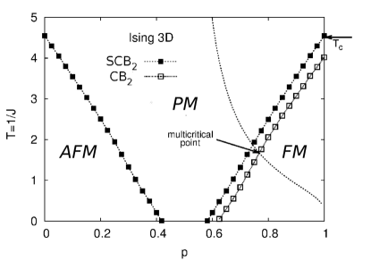
The scaling exponents for the FM fixed point are $y_{T}=1.039$ and $y_{h}=2.487$, see Table 3 for comparison of the corresponding critical exponents. The exponent $\alpha$ is negative, even more than the previous cases, signaling the absence of other fixed points for $1/2\leq p<1$, according to the Harris criterion Harris (1974).

For the AFM critical fixed point we get $y_{T}=1.039$ and $y_{h}=0.6075$, while that of the staggered magnetic field is $y_{h^{\dagger}}=1.487$.

The re-entrance of the transition line below the Nishimori line is missing, confirming also for the 3D case the limitations of the block RG transformation based on the small cluster scheme.

In conclusion, the phase diagram obtained for the 2D and 3D Ising models are qualitatively similar, with the notable absence of any SG phase in the 3D case.

The extension to larger cells, similar to the one discussed in Sec. II.4 for the 2D case, becomes readily unfeasible for 3D lattices. For example with $8$ cubic cells one should sum over the configurations of $4^{3}$ spins, more than $10^{14}$ times the configurations of the two cells cluster.

However, based on the results of the 2D case, we do not expect that such an extension would solve the problem of the SG phase. To catch the SG phase one has to look for different block RG transformation strategies that account for SG local order. In particular, spins could not be right variables to be directly mapped in the RG procedure, since the local magnetization is not a meaningful parameter for the SG phase.

	T${}_{\text{c}}\mathbf{(p=1)}$	p${}_{\text{mc}}$	T${}_{\text{mc}}$
CB2	4.0177	$0.7679\phantom{(x)}$	$1.672\phantom{(x)}$
tCB2	4.5115	$0.7562\phantom{(x)}$	$1.767\phantom{(x)}$
SCB2	4.5537	$0.7445\phantom{(x)}$	$1.870\phantom{(x)}$
3D Ozeki and Ito (1998)	4.5115	$0.7673(4)$	$1.676(3)$

Table 4: Estimate of the FM critical fixed point and of the intersection between the PM/FM transition line with the Nishimori line for the disordered bimodal 3D Ising model obtained using the two cell clusters discussed in the text. In the last line we compare with the values for the 3D Bravais lattice.

IV Cluster Renormalization Group for the Blume-Emery-Griffiths model

In this Section we apply the RG analysis to the BEG model, a spin-$1$ model introduced for the study of the superfluid transition in He³-He⁴ mixtures Blume et al. (1971). The BEG model was originally studied in the mean-field approximation in Refs. [Blume, 1966; Capel, 1966; Blume et al., 1971]. Finite dimensional analysis has been carried out by different means, e.g., series extrapolation techniques Saul et al. (1974), RG analysis Berker and Wortis (1976), Monte Carlo simulations Deserno (1997), effective-field theory Chakraborty (1984) or two-particle cluster approximation Baran and Levitskii (2002). Extensions to quenched disorder, both perturbing the ordered fixed point and in the regime of strong disorder, have been studied throughout the years by means of mean-field approximation Crisanti and Leuzzi (2002); Crisanti and Ritort (2004); Crisanti et al. (2005), real space RG analysis on Migdal-Kadanoff hierarchical lattices Falicov and Berker (1996); Özçelik and Berker (2008) and Monte Carlo numerical simulations Puha and Diep (2000); Paoluzzi et al. (2010, 2011); Leuzzi et al. (2011).

Besides a second order phase transition, the model is known to display a first order phase transition associated with phase separation between the PM and FM phases in the ordered case, and between the PM and SG phases in the quenched disordered case. This rich phase diagram allows for a structured analysis of the RG approximations. In particular, we go through a detailed study of the ordered 2D BEG model, to compare with the results of Ref. Berker and Wortis (1976), and we show the main properties of the quenched disordered 3D BEG model, which is an relevant test model for RG methods of quenched disordered systems.

Fixed point	Type	$\mathbf{J,K,\boldsymbol{\Delta}}$
Higher-order fixed points
$\text{C}^{*}$	Critical	$0.4259,-0.2910,-\infty$
$\text{G}^{*}$	Critical	$0,1.701,4.096$
$\text{L}^{*}$	Critical end	$0.4250,+\infty,+\infty$
$\text{T}^{*}$	Ordinary tricritical	$0.8848,0.9031,3.528$
$\text{P}^{*}$	Special tricritical	$0.4994,1.495,3.992$
First-order fixed points
$\text{Fe}^{*}$	Discontinuous $\mathcalligra{m}$	$+\infty,-\infty,-\infty$
$\text{F}^{*}_{J},\text{F}^{*}_{K},\text{A}^{*}$	Discontinuous $\mathcalligra{m},\,\mathcalligra{q}$	$+\infty,+\infty,+\infty$
$\text{F}^{*}_{2}$	Discontinuous $\mathcalligra{q}$	$0,+\infty,+\infty$
Trivial fixed points
$\text{Pa}^{*}_{+}$	Sink for $\mathcalligra{m}=0$ , large $\mathcalligra{q}$ phase	$0,0,-\infty$
$\text{Pa}^{*}_{-}$	Sink for $\mathcalligra{m}=0$ , small $\mathcalligra{q}$ phase	$0,0,+\infty$
$\text{S}^{*}$	Smooth continuation between $\text{Pa}^{*}_{+}$ and $\text{Pa}^{*}_{-}$	$0,0,\ln 2$

Table 5: Location of all the fixed points of the RG flow for the 2D BEG model obtained with the $\text{SSQ}_{2}$ cluster. The phase transitions are characterize by the magnetization $\mathcalligra{m}\equiv\langle s_{i}\rangle$ and the quadrupole order parameter $\mathcalligra{q}=\langle s_{i}^{2}\rangle$. The notation for the fixed points is the same as in Ref. Berker and Wortis (1976), where their complete description is presented.

IV.1 Ordered 2D BEG model

Following Berker and Wortis Berker and Wortis (1976), in the ordered case we write the BEG Hamiltonian as

$$-\beta{\cal{H}}(\{s\})= J\sum_{\langle ij\rangle}s_{i}s_{j}+K\sum_{\langle ij\rangle}s_{i}^{2}s_{j}^{2}-\Delta\sum_{i}s_{i}^{2}$$

$$+h\sum_{i}s_{i}+L\sum_{\langle ij\rangle}\left(s_{i}s_{j}^{2}+s_{i}^{2}s_{j}\right),$$ (12)

where $s_{i}=0,\pm 1$. As for the Ising model, we are interested in the case $h=L=0$, but these interactions must be still considered for the evaluation of the critical exponents. All the transitions in this model are characterized by two order parameters: the magnetization $\mathcalligra{m}\equiv\langle s_{i}\rangle$ and the quadrupole order parameter $\mathcalligra{q}\equiv\langle s_{i}^{2}\rangle$, giving the density of magnetic or occupied sites.

We stress that the BEG model with $h=L=0$ reduces to the Ising model discussed in the previous Section in two separate regions of the phase diagram: in the limit $\Delta\to-\infty$, where the holes $s_{i}=0$ are trivially suppressed; and on the $J=0$ plane, where the magnetization is zero and the model reduces to the Ising model for the spin variable $u_{i}\equiv 2s_{i}^{2}-1$ in the field $h_{u}=K+(\ln 2-\Delta)/2$. The exact mapping between the region $\Delta\ll-1$ and the line $J=0,\,\Delta=2K+\ln 2$ is known as Griffiths symmetry Griffiths (1967). A basic requirement for our RG transformation is, consequently, to be equivalent in the two regions and to reduce to the one previously defined for the Ising model.

We shall consider the block RG transformation based on the same clusters used for the 2D Ising model, and in particular for the $\text{SQ}_{2}$ cluster we reproduce results coinciding with those of Ref. Berker and Wortis (1976).

The generalization of the cell projection matrix of Sec. II.1 to the spin-1 case is provided by

$$\mathcal{M}(1,s_{i\in c})$$

This is the most general cell projection matrix that contains the up-down, the Griffiths and the square symmetries Berker and Wortis (1976). In particular, for $t=0$ it reduces to the double majority rule: the majority rule is first applied to the variable $u_{i}\equiv 2s_{i}^{2}-1$, and then, if the magnetic sites are dominant, to $s_{i}=\pm 1$.

The block RG transformation leads to the renormalized Hamiltonian for the new spin variables

$$-\beta{\cal H}_{R}(s_{a},s_{b})=\alpha\,\Bigl{[} J_{R}\,s_{a}s_{b}+K_{R}\,s^{2}_{a}s^{2}_{b}+$$ (13)

$$+L_{R}(s_{a}^{2}s_{b}+s_{a}s_{b}^{2})+$$

$$-\Delta_{R}(s_{a}^{2}+s_{b}^{2})+h_{R}(s_{a}+s_{b})\Bigr{]}$$

with

$$J_{R}= \frac{1}{4\alpha}\log\biggl{(}\frac{x_{++}\,x_{--}}{x_{+-}^{2}}\biggl{)}$$

$$K_{R}= \frac{1}{4\alpha}\log\biggl{(}\frac{x_{++}\,x_{--}\,x_{+-}^{2}\,x_{00}^{4}}{x_{+0}^{4}\,x_{-0}^{4}}\biggl{)}$$

$$\Delta_{R}= \frac{1}{2}\log\biggl{(}\frac{x_{00}^{2}}{x_{+0}\,x_{-0}}\biggl{)}$$ (14)

$$L_{R}= \frac{1}{4\alpha}\log\biggl{(}\frac{x_{++}\,x_{-0}^{2}}{x_{--}\,x_{+0}^{2}}\biggl{)}$$

$$h_{R}= \frac{1}{2}\log\biggl{(}\frac{x_{+0}}{x_{-0}}\biggl{)}$$

where $x_{s_{a}s_{b}}$ are the edge factors (6) and $\alpha=4$ for the 2D lattice. Note as in our case $h=L=0$ at the beginning and they are not generated in the RG process. The explicit expressions for $h_{R}$ and $L_{R}$ are nevertheless required to obtain the critical exponents (cfr. Appendix A).

The evaluation of the stability matrix can be problematic if the RG flux flows towards a fixed point where one of the parameters is infinite, e.g., $\Delta\to-\infty$. In cases like this it is more convenient to use a variable remaining finite at the fixed point, e.g., $A=e^{\Delta}$.

The locations of all the fixed points in the RG flow generated by the block RG based on the $\text{SSQ}_{2}$ cluster are reported in Table 5.

The fixed points $\text{C}^{*}$, $\text{G}^{*}$ and $\text{P}^{*}$ are of particular interest for testing the RG procedure because they are known exactly. Moreover, the FM Ising fixed point C^∗ and the Griffiths fixed point G^∗ are related to each other. The first occurs for $\Delta\to-\infty$, while the second at $J=0$, and the Griffiths symmetry Griffiths (1967); Berker and Wortis (1976) imposes the relations

$$K_{\text{G}^{*}}= \,4J_{\text{C}^{*}}\,, \Delta_{\text{G}^{*}}= \,8J_{\text{C}^{*}}+\ln 2.$$ (15)

These relations are verified by our numerical results. The FM fixed point C^∗ can be used to fine tune the value of the parameter $t$ in the projection matrix, obtaining $t=-0.06453$, the same value found for the 2D Ising model, see Sec.II.

The completely unstable Potts fixed point P^∗ can be used as an indicator of the precision of the cluster approximation used in the RG analysis. The position of the point is known to lie on the axis Berker and Wortis (1976)

$$K\,= \,3J\,, \Delta\,= \,8J;$$ (16)

where the Hamiltonian (12) has a three-state permutation symmetry. On this axis the BEG model can be reduced to the three-state Potts model

$$-\beta{\cal{H}}=\mathcal{D}\sum_{\langle ij\rangle}\left(\delta_{s_{i}s_{j}}-1\right)\text{ with }\mathcal{D}=\sqrt{2\frac{J^{2}+K^{2}+\Delta^{2}}{37}}$$

and the critical point of the three-state Potts model is at $\mathcal{D}=\ln(1+\sqrt{3})=1.0050525...$ Berker and Wortis (1976).

The location of the fixed points C^∗, G^∗ and P^∗ are shown in Table 6, and we note as the $\text{SSQ}_{2}$ cluster gives better estimation compared to the $\text{SQ}_{2}$ clusters.

In particular, the location $(J,K,\Delta)$ of the fixed point P^∗ deviates from the exact result of about $(16\%,\,16\%,\,16\%)$ for the $\text{SQ}_{2}$ cluster, of $(6\%,\,2\%,\,0.2\%)$ for the $\text{tSG}_{2}$ with $t=-0.06453$, and of about $(0.6\%,0.8\%,0.7\%)$ for the $\text{SSQ}_{2}$. In terms of $\mathcal{D}$ this translates into $\mathcal{D}=1.1696$ for the $\text{SQ}_{2}$ cluster, $\mathcal{D}=1.001535$ for the $\text{tSQ}_{2}$, and $\mathcal{D}=0.997894$ for the $\text{SSQ}_{2}$.

     $\text{SQ}_{2}$ Berker and Wortis (1976)   $\text{tSQ}_{2}$   SSQ₂   2D $J$ 0.5275 0.4407 0.4259 0.4407 C^∗ $K$ -0.1618 -0.2414 -0.2910 not known $\Delta$ $-\infty$ $-\infty$ $-\infty$ $-\infty$ $J$ 0 0 0 0 G^∗ $K$ 2.110 1.763 1.701 1.763 $\Delta$ 4.913 4.219 4.096 4.219 $J$ 0.5822 0.5319 0.4994 0.5026 P^∗ $K$ 1.756 1.476 1.495 1.508 $\Delta$ 4.678 4.012 3.992 4.020

Table 6: Location of the fixed points C^∗, G^∗ and P^∗ for the ordered 2D BEG model obtained with all the 2 cells cluster discussed in the text compared to the exact results for the 2D lattice.

The projection matrix defined above does not preserve the three-state permutation symmetry on the Potts-axis (16), as an exact RG would do. The distance of the fixed point P^∗ from the Potts-axis can then be used as an indicator of the error made with the cluster approximation used to build the block RG transformation. The distance of $\text{P}^{*}$ from the Potts-axis, over its distance from the origin, turn out to be $6\times 10^{-4}$ for the $\text{SQ}_{2}$ cluster, $10^{-2}$ for the tuned $\text{tSQ}_{2}$ cluster and $4\times 10^{-4}$ for the $\text{SSQ}_{2}$ cluster. Note, specifically, that a strong violation is obtained with the $\text{tSQ}_{2}$ cluster with the “unphysical” negative $t$.

Finally, in Table 7 we show the five scaling exponents for the fixed points $\text{G}^{*}$, $\text{C}^{*}$, $\text{L}^{*}$ and $P^{*}$ (cfr. Appendix A). We stress as the critical exponents obtained with the SSQ₂ cluster approximation are more precise than those obtained with the original square cells cluster SQ₂.

Using, alternatively, the free $t$ trick, the critical exponents are more similar to the known exact ones respect to the staggered cells cluster case. Especially, the exactly known exponents for $\text{C}^{*}$, $\text{G}^{*}$ and $\text{L}^{*}$ are considerably better approached with the tSQ₂ cluster. This is not surprising since $t=-0.06453$ fixes the exact location for $\text{C}^{*}$ (and $\text{G}^{*}$), and we, then, expect that also the estimates of their scaling exponents improve. The known exponents of P^∗ show, instead, only a slight improvement.

    SQ₂ Berker and Wortis (1976)   tSQ₂    SSQ₂    2D $y_{2}$ 0.7267 0.9419 0.7534 1 $y_{4}$ -1.0492 -1.644 -0.2714 $\text{C}^{*}$ $y_{6}$ $-\infty$ $-\infty$ $-\infty$ $y_{1}$ 1.942 1.870 1.839 1.875 $y_{3}$ 0.3792 -0.3556 0.3408 $y_{2}$ 0.7267 0.9419 0.7534 1 $y_{4}$ 1.942 1.870 1.839 1.875 $\text{G}^{*}$ $y_{6}$ -1.834 -1.638 -0.8473 $y_{1}$ 0.5748 0.6628 0.5501 $y_{3}$ -0.7327 -0.6731 -0.5270 $y_{2}$ 0.7267 0.9419 0.7534 1 $y_{4}$ 2.000 2.000 2.000 $\text{L}^{*}$ $y_{6}$ $-\infty$ -0.5095 $-\infty$ $y_{1}$ 1.942 1.870 1.839 1.875 $y_{3}$ 0.2355 -0.3208 0.3428 $y_{2}$ 1.942 1.870 1.854 $1.8\overline{6}$ $y_{4}$ 0.8327 1.106 0.8958 1.2 $P^{*}$ $y_{6}$ 0.4645 0.5248 0.4383 $y_{1}$ 1.936 1.869 1.837 $y_{3}$ 0.3846 0.5304 0.3021

Table 7: Scaling exponents of the fixed points $\text{C}^{*}$, $\text{G}^{*}$, $\text{L}^{*}$ and $\text{P}^{*}$ obtained by means of different cell clusters. The parity of the scaling exponent index refers to the parity of the interaction. The exponent $y_{2C}=y_{2G}=y_{2L}=1$ corresponds to the thermal eigenvalue of the Onsager transition ($y_{T}$), while the exponent $y_{4G}=y_{1C}=y_{1L}=1.875$ corresponds to the magnetic eigenvalue one ($y_{H}$) Berker and Wortis (1976). The exact critical exponents for the $\text{P}^{*}$ fixed point correspond instead to the transition in the three-state Potts model Wu (1982).

IV.2 3D BEG with quenched disorder

In this Section we extend the analysis to the quenched disordered BEG model in three dimensions. The quenched disordered 3D BEG model represents a relevant test for the cluster RG applied to disordered systems. Monte Carlo numerical simulations Paoluzzi et al. (2010) show a critical transition line between the PM phase and a SG phase, which, similar to what found in the mean-field study Crisanti and Leuzzi (2002), consists of a second order transition terminating in a tricritical point from which a first order inverse transition starts. Furthermore, a re-entrance of the first order transition line is present for positive, finite values of the chemical potential of the holes Crisanti et al. (2005), yielding the so-called inverse freezing phenomenon. The real space RG study of Ozcelik and Berker Özçelik and Berker (2008) based on Migdal-Kadanoff cells does not reveal any first order phase transitions, nor any re-entrance. When the real space RG is extended to more structured hierarchical lattices Antenucci et al. (2014) the re-entrance can be recovered, but no tricritical point and first order transition are found.

The Hamiltonian of the disordered BEG model suitable for the RG study is

$$-\beta\mathcal{H}= +\sum_{\left\langle ij\right\rangle}J_{ij}s_{i}s_{j}+\sum_{\left\langle ij\right\rangle}K_{ij}s^{2}_{i}s^{2}_{j}+$$

$$-\sum_{\left\langle ij\right\rangle}\Delta_{ij}\left(s^{2}_{i}+s^{2}_{j}\right)-\sum_{\left\langle ij\right\rangle}\Delta_{ij}^{\dagger}\left(s^{2}_{i}-s^{2}_{j}\right)$$ (17)

where the couplings are quenched random variables with the probability distribution

$$P(\boldsymbol{\mathcal{K}}_{ij})= \bigl{[}(1-p)\,\delta(J_{ij}+J)+p\,\delta(J_{ij}-J)\bigr{]}$$

$$\times\delta\left(K_{ij}-K\right)\delta\left(\Delta_{ij}-\Delta\right)\delta\left(\Delta^{\dagger}_{ij}\right).$$ (18)

If an external field $h$ is added, besides the single site term, one has to include also the odd interaction term $s_{i}s_{j}^{2}$.

The model has been studied using the $\text{CB}_{2}$ cluster shown in Fig. 7 and its staggered version $\text{SCB}_{2}$ using in both cases $N_{s}=10$ pools of size $M=10^{6}$.

Figure 10: Flow of the renormalized probability distribution $P(\boldsymbol{\mathcal{K}})$ for the disordered 3D BEG model in the paramagnetic phase: $J=4$, $K=0$, $\Delta=0.4$ and $p=0.6$ on the SCB₂ cluster. The parameters $K$ and $\Delta^{\dagger}$ are integrated.

Figure 11: Flow of the renormalized probability distribution $P(\boldsymbol{\mathcal{K}})$ for the disordered 3D BEG model in the ferromagnetic phase: $J=4$, $K=0$, $\Delta=0.4$ and $p=0.7$ on the SCB₂ cluster. The parameters $K$ and $\Delta^{\dagger}$ are integrated.

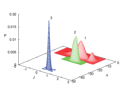
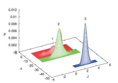
Similar to what seen in the previous Section, only the PM and the FM phases are found, while the SG phase remains undetected in the whole phase diagram. Two typical flows of the probability distribution towards the PM and FM fixed points are shown in Figs. 10 and 11. In the PM phase the average value of $J_{ij}$ goes to zero, while in the FM it moves towards $+\infty$. In both cases the distributions become narrower and narrower under the block RG transformation.

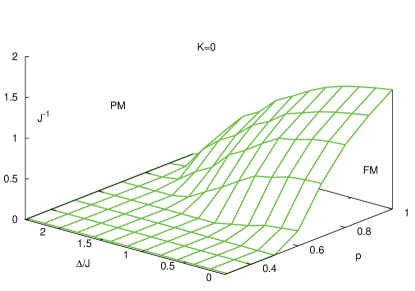
The PM/FM critical surface in the space $(T,\Delta/J,p)$ for the $K=0$ case obtained with the $\text{SCB}_{2}$ cluster is shown in Fig. 12. All the points on the critical surface flow under RG towards one of the two ordered fixed points at $p=1$ with mean value $\mu_{\Delta}\to\pm\infty$ and variance $\sigma^{2}_{\Delta}\to 0$. The analysis of the critical properties is then reduced to the study of an ordered model. In particular the fixed point at $\mu_{\Delta}=-\infty$ corresponds at the critical fixed point of the 3D Ising model discussed in Sec. III.

Figure 12: PM/FM critical surface in the $(T,\Delta/J,p)$ parameter space for the 3D BEG model with $K=0$ obtained with the $\text{SCB}_{2}$ cluster.

V Discussion and conclusions

In this paper we have presented an extension of the real space cluster RG method with two cells proposed by Berker and Wortis Berker and Wortis (1976) by considering a staggered topology for the clusters. This not only makes the antiferromagnetic phase detectable, but leads to an improvement of the estimates of the critical exponents and of the location of the critical points for both the Ising and BEG models.

The two staggered cells cluster appears to be more reliable also with respect to the tuned version of the square cells cluster approach where one, or more, free parameters in the cell projection matrix are fixed by the knowledge of some points in the phase diagrams. The later tuning method is not only less predictive, requiring as input some known points, but it may lead to an “unphysical” projection matrix Berker and Wortis (1976). We have seen, indeed, that in certain cases, for example when fixing the critical temperature of the 2D Ising model to the exact value, the resulting projection matrix assigns a negative contribution to some spin configurations to the partition sum. A choice not providing any physical insight. The staggered cells cluster, instead, is physically motivated: the invariance of an antiferromagnetic ordering under RG. It is remarkable that this request not only allows to study the critical properties of the Neèl transition, but quantitatively improves the results also for the pure ferromagnetic models.

We observe as these results for the pure models are directly valid for a percolation problem: defining an occupation variable as $\epsilon_{12}=(\sigma_{1}\sigma_{2}-1)/2$, the relative percolation threshold is achieved at $p_{c}=1/(1+e^{2\beta_{c}})$.

We have then reported the results of the extension of the cell blocks RG transformation to quenched disordered systems.

We have established that in two dimensions, even in the staggered version, the results are not consistent with exact results for the corresponding regular lattice. In particular, the ferromagnetic phase is detected also beyond the intersection with the Nishimori line. In this case we have also considered the extension to four cells cluster. Although the approximation is not systematic, with a square cell arrangements a clear improvement is achieved in the pure model. We observe that a four cells cluster is the minimal requirement to preserve possible plaquette frustration in presence of bond disorder under the RG process, which is necessary to identify a spin glass critical point (at $T=0$ in 2D). Our investigation shows that the requirement, though necessary, is non sufficient. Indeed, the phase diagram of four cells cluster, besides a minor improvement in the slope of the critical line, shows the same features of the two cells case.

In the three dimensional case, a similar scenario is obtained: in the pure case the staggered version shows a clear improvement, while the quenched disordered extension is ineffective and the expected spin glass phase remains undetected for both the Ising and BEG models.

This failure follows previous attempts of generalizing real space RG methods conceived for ordered systems to disordered systems. The generalization to disordered systems has led in the past to ambiguous results. On the one hand the cumulant expansion Kinzel and Fisher (1978); Tatsumi (1978) has provided evidence for a spin glass phase in dimension $2$, lower than the lower critical dimension $2.5$ Franz et al. (1994); Franz and Toninelli (2005); Boettcher (2005). On the other hand, however, the attempts to extend the block RG transformation on spin clusters did not yield any spin glass fixed point, even in dimension $3$ Kinzel and Fisher (1978).

The lack of a spin glass phase in our scheme is also related to the incorrect location of the boundary of the ferromagnetic phase in the disordered region. We have shown, indeed, that in the disordered Ising model the ferromagnetic phase enters also in the region forbidden by Nishimori’s gauge theory. This occurs with all clusters used. The problem is only partly mitigate when the tuned cluster is used, cfr. Figs. 3 and 8, and its uncontrolled nature does not allow for any further physical insight. A milder, but more recognizable attenuation, is obtained with the four cells cluster, cfr. Fig. 4. In this regard we stress here that the correlation generated by the RG transformation among different types of couplings cannot be disregarded. In particular, taking the naive approximation $P(J,K,\Delta)\simeq P(J)P(K)P(\Delta)$, and so using three independent pools for the three kinds of interaction, the PM/FM transition line becomes straight, not different from what found with the SQ₂ cell. Nevertheless, our analysis shows that parameter correlation is only one of the necessary ingredients, and that the limitations of the block RG study of disordered models are not due to the truncation process of the interactions, but mostly to the nature itself of the block cells construction.

The connection between the problem in the ferromagnetic critical line and the detection of the spin glass phase is highlighted by looking at the single RG flow: the variance $\sigma^{2}_{J}$ of the probability distributions goes quickly to zero in all the detected phases. This does not happen, for example, in the real space RG on hierarchical lattice Antenucci et al. (2014) where the variance $\sigma^{2}_{J}$ of the couplings increases in the FM phase, even though $\sigma_{J}/\mu_{J}\to 0$, and the spin glass phase is detected as the region of the phase diagram where $\sigma_{J}/\mu_{J}\to\infty$. It is clear that, in order to build a valuable generalization of the RG cluster method to strong disorder, the first step is to obtain the correct evolution of the FM phase for weak disorder.

Further issues take place when the extension to strong disorder is considered. In particular, the improvement achieved with the staggered cells clusters shows as, to correctly detect the antiferromagnetic phase, it is essential that the ground state of the system is invariant under the RG transformation. In the strong disorder regime this requirement becomes harder to satisfy, as the frustration causes a proliferation of nontrivial degenerate ground states.

The present analysis makes eventually clear that, while the cell blocks RG method works well for pure, ferromagnetic or antiferromagnetic, systems, the generalization to the case of strong disorder calls for a different procedure for the block RG transformation.

The renormalization via the majority rule, or its tuned improvement, yields a local magnetization of the coarse grained cell. This is meaningful as far as magnetization is the relevant order parameter of the transition. In the spin-glass transition, though, magnetization is zero and the relevant order parameter is the “replica” overlap. The overlap allows, in particular, to take into account the ergodicity breaking caused by frustration, as it may translate into the replica symmetry breaking of the appropriate overlap probability distribution. To put forward a renormalization procedure based on the overlap coarse graining one has, thus, to resort to replicated clusters. More instances of the system should, then, be renormalized together via the value of the mutual overlap. Such a generalization, and its numerically feasible implementation, is currently under investigation.

Appendix A RG Stability Matrix for the BEG model

The critical exponents are obtained from the eigenvalue of the stability matrix $\partial\boldsymbol{\mathcal{K}}_{R}/\partial\boldsymbol{\mathcal{K}}$ evaluated at the fixed point $\boldsymbol{\mathcal{K}}^{*}$. For the BEG model $\boldsymbol{\mathcal{K}}=\{J,K,\Delta,L,h\}$ and the elements of the stability matrix are

$$\frac{\partial J_{R}}{\partial\boldsymbol{\mathcal{K}}}\! =\!\frac{1}{4\alpha}\!\left(\frac{x_{++}^{\prime}}{x_{++}}+\frac{x_{--}^{\prime}}{x_{--}}-\frac{2x_{+-}^{\prime}}{x_{+-}}\right)$$

$$\frac{\partial K_{R}}{\partial\boldsymbol{\mathcal{K}}}\! =\!\frac{1}{4\alpha}\!\left(\frac{x_{++}^{\prime}}{x_{++}}+\frac{x_{--}^{\prime}}{x_{--}}+\frac{2x_{+-}^{\prime}}{x_{+-}}\right.$$

$$\qquad\qquad\left.+\frac{4x_{00}^{\prime}}{x_{00}}-\frac{4x_{+0}^{\prime}}{x_{+0}}-\frac{4x_{-0}^{\prime}}{x_{-0}}\right)$$

$$\frac{\partial\Delta_{R}}{\partial\boldsymbol{\mathcal{K}}}\! =\!\frac{1}{2}\!\left(\frac{x_{+0}^{\prime}}{x_{+0}}+\frac{x_{-0}^{\prime}}{x_{-0}}-\frac{2x_{00}^{\prime}}{x_{00}}\right)$$

$$\frac{\partial L_{R}}{\partial\boldsymbol{\mathcal{K}}}\! =\!\frac{1}{4\alpha}\!\left(\frac{x_{++}^{\prime}}{x_{++}}+\frac{2x_{-0}^{\prime}}{x_{-0}}-\frac{x_{--}^{\prime}}{x_{--}}-\frac{2x_{+0}^{\prime}}{x_{+0}}\right)$$

$$\frac{\partial h_{R}}{\partial\boldsymbol{\mathcal{K}}}\! =\!\frac{1}{4}\!\left(\frac{x_{+0}^{\prime}}{x_{+0}}-\frac{x_{-0}^{\prime}}{x_{-0}}\right)$$

where $x_{\sigma_{a}\sigma_{b}}^{\prime}=\partial x_{\sigma_{a}\sigma_{b}}/\partial\boldsymbol{\mathcal{K}}$ and $\alpha=2d$, with $d$ the space dimension. The derivative of the Boltzmann factors can be expressed as

$$\frac{\partial x_{\sigma_{a}\sigma_{b}}}{\partial J} =\sum_{\bm{s}}\mathcal{M}_{a}\mathcal{M}_{b}\left[\alpha\sum_{\langle ij\rangle}s_{i}s_{j}\right]e^{-\beta{\cal{H}}(\bm{s})}$$

$$\frac{\partial x_{\sigma_{a}\sigma_{b}}}{\partial K} =\sum_{\bm{s}}\mathcal{M}_{a}\mathcal{M}_{b}\left[\alpha\sum_{\langle ij\rangle}s_{i}^{2}s_{j}^{2}\right]e^{-\beta{\cal{H}}(\bm{s})}$$

$$\frac{\partial x_{\sigma_{a}\sigma_{b}}}{\partial D} =\sum_{\bm{s}}\mathcal{M}_{a}\mathcal{M}_{b}\left[-\sum_{i}s_{i}^{2}\right]e^{-\beta{\cal{H}}(\bm{s})}$$

$$\frac{\partial x_{\sigma_{a}\sigma_{b}}}{\partial L} =\sum_{\bm{s}}\mathcal{M}_{a}\mathcal{M}_{b}\left[\alpha\sum_{\langle ij\rangle}(s_{i}^{2}s_{j}+s_{i}s_{j}^{2})\right]e^{-\beta{\cal{H}}(\bm{s})}$$

$$\frac{\partial x_{\sigma_{a}\sigma_{b}}}{\partial h} =\sum_{\bm{s}}\mathcal{M}_{a}\mathcal{M}_{b}\left[\sum_{i}s_{i}\right]e^{-\beta{\cal{H}}(\bm{s})}$$

where $\mathcal{M}_{x}\equiv\mathcal{M}(\sigma_{x},s_{i\in x})$ are the cell projection matrices.

When the fixed point is at $L=h=0$ the even and odd couplings decouples and the stability matrix is block-diagonal, with a $3\times 3$ block for even couplings and a $2\times 2$ block for odd ones.

The scaling exponents controlling the stability of the fixed point are $y_{i}=\log_{b}\lambda_{i}$, where $\lambda_{i}$ are the eigenvalues of the stability matrix evaluated at the fixed point, and $b$ the scaling factor of the RG scheme, $b=2$ in this work.

References

- Kaufman and Griffiths (1981) M. Kaufman and R. B. Griffiths, Phys. Rev. B 24, 496 (1981).
- Griffiths and Kaufman (1982) R. B. Griffiths and M. Kaufman, Phys. Rev. B 26, 5022 (1982).
- Salmon et al. (2010) O. R. Salmon, B. T. Agostini, and F. D. Nobre, Physics Letters A 374, 1631 (2010).
- Antenucci et al. (2014) F. Antenucci, A. Crisanti, and L. Leuzzi, Journal of Statistical Physics 155, 909 (2014), ISSN 0022-4715.
- Niemeijer and Leeuwen (1973) T. Niemeijer and J. M. J. Leeuwen, Phys. Rev. Lett. 31, 1411 (1973).
- Berker and Wortis (1976) A. N. Berker and M. Wortis, Physical Review B 14, 4946 (1976).
- Reynolds et al. (1977) P. J. Reynolds, H. E. Stanley, and W. Klein, Journal of Physics C: Solid State Physics 10, L167 (1977).
- Reynolds et al. (1978) P. J. Reynolds, H. E. Stanley, and W. Klein, Journal of Physics A: Mathematical and General 11, L199 (1978).
- Nishimori (2001) H. Nishimori, Statistical Physics of Spin Glasses and Information Processing: An Introduction (Oxford University Press (Oxford), 2001).
- Nienhuis and Nauenberg (1975) B. Nienhuis and M. Nauenberg, Phys. Rev. Lett. 35, 477 (1975).
- Onsager (1943) L. Onsager, Phys. Rev. 65, 117 (1943).
- Southern and Young (1977) B. W. Southern and A. P. Young, Journal of Physics C 10, 2179 (1977).
- Nobre (2001) F. D. Nobre, Physical Review E 64, 046108 (2001).
- Nishimori (1981) H. Nishimori, Prog. Theor. Phys. 66, 1169 (1981).
- Harris (1974) A. B. Harris, J. Phys. C: Sol. St. Phys. 7, 1671 (1974).
- Toldin et al. (2009) F. P. Toldin, A. Pelissetto, and E. Vicari, JSTAT 135, 1039 (2009).
- Hasenbusch et al. (2008) M. Hasenbusch, F. P. Toldin, A. Pelissetto, and E. Vicari, Phys. Rev. E 77, 051115 (2008).
- Ohzeki (2009) M. Ohzeki, Phys. Rev. E 79, 021129 (2009).
- Talapov and Blöte (1996) A. L. Talapov and H. W. J. Blöte, J. of Phys. A 29, 5727 (1996).
- Pelissetto and Vicari (2002) A. Pelissetto and E. Vicari, Phys. Rep. 368, 549 (2002).
- Ozeki and Ito (1998) Y. Ozeki and N. Ito, Journal of Physics A: Mathematical and General 31, 5451 (1998).
- Blume et al. (1971) M. Blume, V. J. Emery, and R. B. Griffiths, Phys. Rev. A 4, 1071 (1971).
- Blume (1966) M. Blume, Phys. Rev. 141, 517 (1966).
- Capel (1966) H. W. Capel, Physica 32, 966 (1966).
- Saul et al. (1974) D. M. Saul, M. Wortis, and D. Stauffer, Phys. Rev. B 9, 4964 (1974).
- Deserno (1997) M. Deserno, Phys. Rev. E 56, 5204 (1997).
- Chakraborty (1984) K. G. Chakraborty, Phys. Rev. B 29, 1454 (1984).
- Baran and Levitskii (2002) O. R. Baran and R. R. Levitskii, Phys. Rev. B 65, 172407 (2002).
- Crisanti and Leuzzi (2002) A. Crisanti and L. Leuzzi, Phys. Rev. Lett. 89, 237204 (2002).
- Crisanti and Ritort (2004) A. Crisanti and F. Ritort, Europhys. Lett. 66, 253 (2004).
- Crisanti et al. (2005) A. Crisanti, L. Leuzzi, and T. Rizzo, Phys. Rev. B 71, 094202 (2005).
- Falicov and Berker (1996) A. Falicov and A. N. Berker, Phys. Rev. Lett. 76, 4380 (1996).
- Özçelik and Berker (2008) V. O. Özçelik and A. N. Berker, Phys. Rev. E 78, 031104 (2008).
- Puha and Diep (2000) I. Puha and H. T. Diep, J. Mag. Mag. Mat. 224, 85 (2000).
- Paoluzzi et al. (2010) M. Paoluzzi, L. Leuzzi, and A. Crisanti, Phys. Rev. Lett. 104, 120602 (2010).
- Paoluzzi et al. (2011) M. Paoluzzi, L. Leuzzi, and A. Crisanti, Philos. Mag. 91, 1966 (2011).
- Leuzzi et al. (2011) L. Leuzzi, M. Paoluzzi, and A. Crisanti, Phys. Rev. B 83, 014107 (2011).
- Griffiths (1967) R. Griffiths, Physica 33, 689 (1967).
- Wu (1982) F. Y. Wu, Rev. Mod. Phys. 54, 235 (1982).
- Kinzel and Fisher (1978) W. Kinzel and F. H. Fisher, J. Phys. C 11, 2115 (1978).
- Tatsumi (1978) T. Tatsumi, Prog. Theor. Phys. 59, 405 (1978).
- Franz et al. (1994) S. Franz, G. Parisi, and M.-A. Virasoro, J. Phys. I (France) 4, 1657 (1994).
- Franz and Toninelli (2005) S. Franz and F. Toninelli, J. Stat. Mech. p. P01008 (2005).
- Boettcher (2005) S. Boettcher, Phys. Rev. Lett. 95, 197205 (2005).