Exact Post Model Selection Inference for Marginal Screening

Jason D. Lee and Jonathan E. Taylor
Abstract

We develop a framework for post model selection inference, via marginal screening, in linear regression. At the core of this framework is a result that characterizes the exact distribution of linear functions of the response y๐‘ฆy, conditional on the model being selected (โ€œcondition on selectionโ€ framework). This allows us to construct valid confidence intervals and hypothesis tests for regression coefficients that account for the selection procedure. In contrast to recent work in high-dimensional statistics, our results are exact (non-asymptotic) and require no eigenvalue-like assumptions on the design matrix X๐‘‹X. Furthermore, the computational cost of marginal regression, constructing confidence intervals and hypothesis testing is negligible compared to the cost of linear regression, thus making our methods particularly suitable for extremely large datasets. Although we focus on marginal screening to illustrate the applicability of the condition on selection framework, this framework is much more broadly applicable. We show how to apply the proposed framework to several other selection procedures including orthogonal matching pursuit, non-negative least squares, and marginal screening+Lasso.

1 Introduction

Consider the model

yi=ฮผโ€‹(xi)+ฯตi,ฯตiโˆผ๐’ฉโ€‹(0,ฯƒ2โ€‹I),formulae-sequencesubscript๐‘ฆ๐‘–๐œ‡subscript๐‘ฅ๐‘–subscriptitalic-ฯต๐‘–similar-tosubscriptitalic-ฯต๐‘–๐’ฉ0superscript๐œŽ2๐ผ\displaystyle y_{i}=\mu(x_{i})+\epsilon_{i},\;\epsilon_{i}\sim\mathcal{N}(0,\sigma^{2}I), (1)

where ฮผโ€‹(x)๐œ‡๐‘ฅ\mu(x) is an arbitrary function, and xiโˆˆ๐‘psubscript๐‘ฅ๐‘–superscript๐‘๐‘x_{i}\in\mathbf{R}^{p}. Our goal is to perform inference on (XTโ€‹X)โˆ’1โ€‹XTโ€‹ฮผsuperscriptsuperscript๐‘‹๐‘‡๐‘‹1superscript๐‘‹๐‘‡๐œ‡(X^{T}X)^{-1}X^{T}\mu, which is the best linear predictor of ฮผ๐œ‡\mu. In the classical setting of n>p๐‘›๐‘n>p , the least squares estimator

ฮฒ^=(XTโ€‹X)โˆ’1โ€‹XTโ€‹y^๐›ฝsuperscriptsuperscript๐‘‹๐‘‡๐‘‹1superscript๐‘‹๐‘‡๐‘ฆ\displaystyle\hat{\beta}=(X^{T}X)^{-1}X^{T}y (2)

is a commonly used estimator for (XTโ€‹X)โˆ’1โ€‹XTโ€‹ฮผsuperscriptsuperscript๐‘‹๐‘‡๐‘‹1superscript๐‘‹๐‘‡๐œ‡(X^{T}X)^{-1}X^{T}\mu. Under the linear model assumption ฮผ=Xโ€‹ฮฒ0๐œ‡๐‘‹superscript๐›ฝ0\mu=X\beta^{0}, the exact distribution of ฮฒ^^๐›ฝ\hat{\beta} is

ฮฒ^โˆผ๐’ฉโ€‹(ฮฒ0,ฯƒ2โ€‹(XTโ€‹X)โˆ’1).similar-to^๐›ฝ๐’ฉsuperscript๐›ฝ0superscript๐œŽ2superscriptsuperscript๐‘‹๐‘‡๐‘‹1\displaystyle\hat{\beta}\sim\mathcal{N}(\beta^{0},\sigma^{2}(X^{T}X)^{-1}). (3)

Using the normal distribution, we can test the hypothesis H0:ฮฒj0=0:subscript๐ป0subscriptsuperscript๐›ฝ0๐‘—0H_{0}:\beta^{0}_{j}=0 and form confidence intervals for ฮฒj0subscriptsuperscript๐›ฝ0๐‘—\beta^{0}_{j} using the z-test.

However in the high-dimensional p>n๐‘๐‘›p>n setting, the least squares estimator is an underdetermined problem, and the predominant approach is to perform variable selection or model selection [3]. There are many approaches to variable selection including AIC/BIC, greedy algorithms such as forward stepwise regression, orthogonal matching pursuit, and regularization methods such as the Lasso. The focus of this paper will be on the model selection procedure known as marginal screening, which selects the k๐‘˜k most correlated features xjsubscript๐‘ฅ๐‘—x_{j} with the response y๐‘ฆy.

Marginal screening is the simplest and most commonly used of the variable selection procedures [13, 28, 20]. Marginal screening requires only Oโ€‹(nโ€‹p)๐‘‚๐‘›๐‘O(np) computation and is several orders of magnitude faster than regularization methods such as the Lasso; it is extremely suitable for extremely large datasets where the Lasso may be computationally intractable to apply. Furthermore, the selection properties are comparable to the Lasso [12]. In the ultrahigh dimensional setting p=Oโ€‹(enk)๐‘๐‘‚superscript๐‘’superscript๐‘›๐‘˜p=O(e^{n^{k}}), marginal screening is shown to have the SURE screening property, P(SโŠ‚S^P(S\subset\hat{S}), that is marginal screening selects a superset of the truly relevant variables [9, 11, 10]. Marginal screening can also be combined with a second variable selection procedure such as the Lasso to further reduce the dimensionality; our statistical inference methods extend to the Marginal Screening+Lasso method.

Since marginal screening utilizes the response variable y๐‘ฆy, the confidence intervals and statistical tests based on the distribution in (3) are not valid; confidence intervals with nominal 1โˆ’ฮฑ1๐›ผ1-\alpha coverage may no longer cover at the advertised level:

Prโก(ฮฒj0โˆˆC1โˆ’ฮฑโ€‹(x))<1โˆ’ฮฑ.Prsubscriptsuperscript๐›ฝ0๐‘—subscript๐ถ1๐›ผ๐‘ฅ1๐›ผ\Pr\left(\beta^{0}_{j}\in C_{1-\alpha}(x)\right)<1-\alpha.

Several authors have previously noted this problem including recent work in [17, 18, 19, 2]. A major line of work [17, 18, 19] has described the difficulty of inference post model selection: the distribution of post model selection estimates is complicated and cannot be approximated in a uniform sense by their asymptotic counterparts.

In this paper, we describe how to form exact confidence intervals for linear regression coefficients post model selection. We assume the model (1), and operate under the fixed design matrix X๐‘‹X setting. The linear regression coefficients constrained to a subset of variables S๐‘†S is linear in ฮผ๐œ‡\mu, ejTโ€‹(XSTโ€‹XS)โˆ’1โ€‹XSTโ€‹ฮผ=ฮทTโ€‹ฮผsuperscriptsubscript๐‘’๐‘—๐‘‡superscriptsuperscriptsubscript๐‘‹๐‘†๐‘‡subscript๐‘‹๐‘†1superscriptsubscript๐‘‹๐‘†๐‘‡๐œ‡superscript๐œ‚๐‘‡๐œ‡e_{j}^{T}(X_{S}^{T}X_{S})^{-1}X_{S}^{T}\mu=\eta^{T}\mu for some ฮท๐œ‚\eta. We derive the conditional distribution of ฮทTโ€‹ysuperscript๐œ‚๐‘‡๐‘ฆ\eta^{T}y for any vector ฮท๐œ‚\eta, so we are able to form confidence intervals and test regression coefficients.

In Section 2 we discuss related work on high-dimensional statistical inference, and Section 3 introduces the marginal screening algorithm and shows how z intervals may fail to have the correct coverage properties. Section 4 and 5 show how to represent the marginal screening selection event as constraints on y๐‘ฆy, and construct pivotal quantities for the truncated Gaussian. Section 6 uses these tools to develop valid hypothesis tests and confidence intervals.

Although the focus of this paper is on marginal screening, the โ€œcondition on selectionโ€ framework, first proposed for the Lasso in [16], is much more general; we use marginal screening as a simple and clean illustration of the applicability of this framework. In Section 7, we discuss several extensions including how to apply the framework to other variable/model selection procedures and to nonlinear regression problems. Section 7 covers

  1. 1.

    marginal screening+Lasso, a screen and clean procedure that first uses marginal screening and cleans with the Lasso,

  2. 2.

    orthogonal matching pursuit (OMP)

  3. 3.

    non-negative least squares (NNLS).

2 Related Work

Most of the theoretical work on high-dimensional linear models focuses on consistency. Such results establish, under restrictive assumptions on X๐‘‹X, the Lasso ฮฒ^^๐›ฝ\hat{\beta} is close to the unknown ฮฒ0superscript๐›ฝ0\beta^{0} [24] and selects the correct model [33, 30, 15]. We refer to the reader to [3] for a comprehensive discussion about the theoretical properties of the Lasso.

There is also recent work on obtaining confidence intervals and significance testing for penalized M-estimators such as the Lasso. One class of methods uses sample splitting or subsampling to obtain confidence intervals and p-values [31, 23]. In the post model selection literature, the recent work of [2] proposed the POSI approach, a correction to the usual t-test confidence intervals by controlling the familywise error rate for all parameters in any possible submodel. The POSI approach will produce valid confidence intervals for any possible model selection procedure; however for a given model selection procedure such as marginal regression, it will be conservative. In addition, the POSI methodology is extremely computationally intensive and currently only applicable for pโ‰ค30๐‘30p\leq 30.

A separate line of work establishes the asymptotic normality of a corrected estimator obtained by โ€œinvertingโ€ the KKT conditions [29, 32, 14]. The corrected estimator b^^๐‘\hat{b} has the form b^=ฮฒ^+ฮปโ€‹ฮ˜^โ€‹z^,^๐‘^๐›ฝ๐œ†^ฮ˜^๐‘ง\hat{b}=\hat{\beta}+\lambda\hat{\Theta}\hat{z}, where z^^๐‘ง\hat{z} is a subgradient of the penalty at ฮฒ^^๐›ฝ\hat{\beta} and ฮ˜^^ฮ˜\hat{\Theta} is an approximate inverse to the Gram matrix XTโ€‹Xsuperscript๐‘‹๐‘‡๐‘‹X^{T}X. The two main drawbacks to this approach are 1) the confidence intervals are valid only when the M-estimator is consistent, and thus require restricted eigenvalue conditions on X๐‘‹X, 2) obtaining ฮ˜^^ฮ˜\hat{\Theta} is usually much more expensive than obtaining ฮฒ^^๐›ฝ\hat{\beta}, and 3) the method is specific to regularized estimators, and does not extend to marginal screening, forward stepwise, and other variable selection methods.

Most closely related to our work is the โ€œcondition on selectionโ€ framework laid out in [16] for the Lasso. Our work extends this methodology to other variable selection methods such as marginal screening, marginal screening followed by the Lasso (marginal screening+Lasso), orthogonal matching pursuit, and non-negative least squares. The primary contribution of this work is the observation that many model selection methods, including marginal screening and Lasso, lead to โ€œselection eventsโ€ that can be represented as a set of constraints on the response variable y๐‘ฆy. By conditioning on the selection event, we can characterize the exact distribution of ฮทTโ€‹ysuperscript๐œ‚๐‘‡๐‘ฆ\eta^{T}y. This paper focuses on marginal screening, since it is the simplest of variable selection methods, and thus the applicability of the โ€œconditioning on selection eventโ€ framework is most transparent. However, this framework is not limited to marginal screening and can be applied to a wide a class of model selection procedures including greedy algorithms such as matching pursuit and orthogonal matching pursuit. We discuss some of these possible extensions in Section 7, but leave a thorough investigation to future work.

A remarkable aspect of our work is that we only assume X๐‘‹X is in general position, and the test is exact, meaning the distributional results are true even under finite samples. By extension, we do not make any assumptions on n๐‘›n and p๐‘p, which is unusual in high-dimensional statistics [3]. Furthermore, the computational requirements of our test are negligible compared to computing the linear regression coefficients.

Our test assumes that the noise variance ฯƒ2superscript๐œŽ2\sigma^{2} is known. However, there are many methods for estimating ฯƒ2superscript๐œŽ2\sigma^{2} in high dimensions. A data splitting technique is used in [8], while [27] proposes a method that computes the regression estimate and an estimate of the variance simultaneously. We refer the reader to [25] for a survey and comparison of the various methods, and assume ฯƒ2superscript๐œŽ2\sigma^{2} is known for the remainder of the paper.

3 Marginal Screening

Let Xโˆˆโ„nร—p๐‘‹superscriptโ„๐‘›๐‘X\in\mathbb{R}^{n\times p} be the design matrix, yโˆˆโ„n๐‘ฆsuperscriptโ„๐‘›y\in\mathbb{R}^{n} the response variable, and assume the model

yi=ฮผโ€‹(xi)+ฯตi,ฯตiโˆผ๐’ฉโ€‹(0,ฯƒ2โ€‹I).formulae-sequencesubscript๐‘ฆ๐‘–๐œ‡subscript๐‘ฅ๐‘–subscriptitalic-ฯต๐‘–similar-tosubscriptitalic-ฯต๐‘–๐’ฉ0superscript๐œŽ2๐ผy_{i}=\mu(x_{i})+\epsilon_{i},\epsilon_{i}\sim\mathcal{N}(0,\sigma^{2}I).

We will assume that X๐‘‹X is in general position and has unit norm columns. The algorithm estimates ฮฒ^^๐›ฝ\hat{\beta} via Algorithm 1.

Algorithm 1 Marginal screening algorithm
1:Input: Design matrix X๐‘‹X, response y๐‘ฆy, and model size k๐‘˜k.
2:Compute |XTโ€‹y|superscript๐‘‹๐‘‡๐‘ฆ|X^{T}y|.
3:Let S^^๐‘†\hat{S} be the index of the k๐‘˜k largest entries of |XTโ€‹y|superscript๐‘‹๐‘‡๐‘ฆ|X^{T}y|.
4:Compute ฮฒ^S^=(XS^Tโ€‹XS^)โˆ’1โ€‹XS^Tโ€‹ysubscript^๐›ฝ^๐‘†superscriptsuperscriptsubscript๐‘‹^๐‘†๐‘‡subscript๐‘‹^๐‘†1superscriptsubscript๐‘‹^๐‘†๐‘‡๐‘ฆ\hat{\beta}_{\hat{S}}=(X_{\hat{S}}^{T}X_{\hat{S}})^{-1}X_{\hat{S}}^{T}y

The marginal screening algorithm chooses the k๐‘˜k variables with highest absolute dot product with y๐‘ฆy, and then fits a linear model over those k๐‘˜k variables. We will assume kโ‰คminโก(n,p)๐‘˜๐‘›๐‘k\leq\min(n,p). For any fixed subset of variables S๐‘†S, the distribution of ฮฒ^S=(XSTโ€‹XS)โˆ’1โ€‹XSTโ€‹ysubscript^๐›ฝ๐‘†superscriptsuperscriptsubscript๐‘‹๐‘†๐‘‡subscript๐‘‹๐‘†1superscriptsubscript๐‘‹๐‘†๐‘‡๐‘ฆ\hat{\beta}_{S}=(X_{S}^{T}X_{S})^{-1}X_{S}^{T}y is

ฮฒ^Ssubscript^๐›ฝ๐‘†\displaystyle\hat{\beta}_{S} โˆผ๐’ฉโ€‹(ฮฒSโ‹†,ฯƒ2โ€‹(XSTโ€‹XS)โˆ’1)similar-toabsent๐’ฉsubscriptsuperscript๐›ฝโ‹†๐‘†superscript๐œŽ2superscriptsuperscriptsubscript๐‘‹๐‘†๐‘‡subscript๐‘‹๐‘†1\displaystyle\sim\mathcal{N}(\beta^{\star}_{S},\sigma^{2}(X_{S}^{T}X_{S})^{-1}) (4)
ฮฒSโ‹†subscriptsuperscript๐›ฝโ‹†๐‘†\displaystyle\beta^{\star}_{S} :=(XSTโ€‹XS)โˆ’1โ€‹XSTโ€‹ฮผ.assignabsentsuperscriptsuperscriptsubscript๐‘‹๐‘†๐‘‡subscript๐‘‹๐‘†1superscriptsubscript๐‘‹๐‘†๐‘‡๐œ‡\displaystyle:=(X_{S}^{T}X_{S})^{-1}X_{S}^{T}\mu. (5)

We will use the notation ฮฒjโˆˆSโ‹†:=(ฮฒSโ‹†)jassignsubscriptsuperscript๐›ฝโ‹†๐‘—๐‘†subscriptsubscriptsuperscript๐›ฝโ‹†๐‘†๐‘—\beta^{\star}_{j\in S}:=\left(\beta^{\star}_{S}\right)_{j}, where j๐‘—j is indexing a variable in the set S๐‘†S. The z-test intervals for a regression coefficient are

Cโ€‹(ฮฑ,j,S):=assign๐ถ๐›ผ๐‘—๐‘†absent\displaystyle C(\alpha,j,S):=
(ฮฒ^jโˆˆSโˆ’ฯƒโ€‹z1โˆ’ฮฑ/2โ€‹(XSTโ€‹XS)jโ€‹j,ฮฒ^jโˆˆS+ฯƒโ€‹z1โˆ’ฮฑ/2โ€‹(XSTโ€‹XS)jโ€‹j)subscript^๐›ฝ๐‘—๐‘†๐œŽsubscript๐‘ง1๐›ผ2subscriptsuperscriptsubscript๐‘‹๐‘†๐‘‡subscript๐‘‹๐‘†๐‘—๐‘—subscript^๐›ฝ๐‘—๐‘†๐œŽsubscript๐‘ง1๐›ผ2subscriptsuperscriptsubscript๐‘‹๐‘†๐‘‡subscript๐‘‹๐‘†๐‘—๐‘—\displaystyle\left(\hat{\beta}_{j\in S}-\sigma z_{1-\alpha/2}(X_{S}^{T}X_{S})_{jj},\hat{\beta}_{j\in S}+\sigma z_{1-\alpha/2}(X_{S}^{T}X_{S})_{jj}\right) (6)

and each interval has 1โˆ’ฮฑ1๐›ผ1-\alpha coverage, meaning Prโก(ฮฒjโˆˆSโ‹†โˆˆCโ€‹(ฮฑ,j,S))=1โˆ’ฮฑPrsubscriptsuperscript๐›ฝโ‹†๐‘—๐‘†๐ถ๐›ผ๐‘—๐‘†1๐›ผ\Pr\left(\beta^{\star}_{j\in S}\in C(\alpha,j,S)\right)=1-\alpha. However if S^^๐‘†\hat{S} is chosen using a model selection procedure that depends on y๐‘ฆy, the distributional result (5) no longer holds and the z-test intervals will not cover at the 1โˆ’ฮฑ1๐›ผ1-\alpha level. It is possible that

Prโก(ฮฒjโˆˆS^โ‹†โˆˆCโ€‹(ฮฑ,j,S^))<1โˆ’ฮฑ.Prsubscriptsuperscript๐›ฝโ‹†๐‘—^๐‘†๐ถ๐›ผ๐‘—^๐‘†1๐›ผ\Pr\left(\beta^{\star}_{j\in\hat{S}}\in C(\alpha,j,\hat{S})\right)<1-\alpha.

Similarly, the test of the hypothesis H0:ฮฒjโˆˆS^โ‹†=0:subscript๐ป0subscriptsuperscript๐›ฝโ‹†๐‘—^๐‘†0H_{0}:\beta^{\star}_{j\in\hat{S}}=0 will not control type I error at level ฮฑ๐›ผ\alpha, meaning Prโก(rejectย H0|H0)>ฮฑPrconditionalrejectย H0subscript๐ป0๐›ผ\Pr\left(\text{reject $H_{0}$}|H_{0}\right)>\alpha.

3.1 Failure of z-test confidence intervals

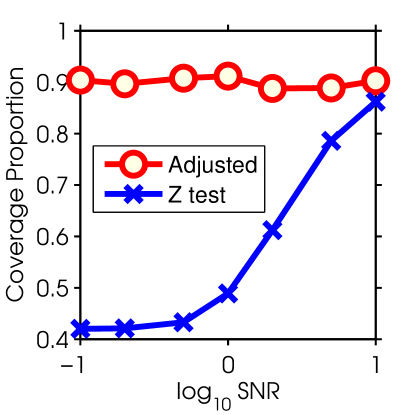
We will illustrate empirically that the z-test intervals do not cover at 1โˆ’ฮฑ1๐›ผ1-\alpha when S^^๐‘†\hat{S} is chosen by marginal screening in Algorithm 1.
Refer to caption
Figure 1: Plots of the coverage proportion across a range of SNR (log-scale). We see that the coverage proportion of the z intervals can be far below the nominal level of 1โˆ’ฮฑ=.91๐›ผ.91-\alpha=.9, even at SNR =5. The adjusted intervals always have coverage proportion .9.9.9.

For this experiment we generated X๐‘‹X from a standard normal with n=20๐‘›20n=20 and p=200๐‘200p=200. The signal vector is 222 sparse with ฮฒ10,ฮฒ20=SNRsubscriptsuperscript๐›ฝ01subscriptsuperscript๐›ฝ02SNR\beta^{0}_{1},\beta^{0}_{2}=\text{SNR}, y=Xโ€‹ฮฒ0+ฯต๐‘ฆ๐‘‹superscript๐›ฝ0italic-ฯตy=X\beta^{0}+\epsilon, and ฯตโˆผNโ€‹(0,1)similar-toitalic-ฯต๐‘01\epsilon\sim N(0,1). The confidence intervals were constructed for the k=2๐‘˜2k=2 variables selected by the marginal screening algorithm. The z-test intervals were constructed via (6) with ฮฑ=.1๐›ผ.1\alpha=.1, and the adjusted intervals were constructed using Algorithm 3. The results are described in Figure 1. The y-axis plots the coverage proportion or the fraction of times the true parameter value fell in the confidence interval. Each point represents 500500500 independent trials. The x-axis varies the SNR parameter over the values 0.1,.2,.5,1,2,5,100.1.2.5125100.1,.2,.5,1,2,5,10. From the figure, we see that the z intervals can have coverage proportion drastically less than the nominal level of 1โˆ’ฮฑ=.91๐›ผ.91-\alpha=.9, and only for SNR=101010 does the coverage tend to .9.9.9. This motivates the need for intervals that have the correct coverage proportion after model selection.

4 Representing the selection event

Since Equation (5) does not hold for a selected S^^๐‘†\hat{S} when the selection procedure depends on y๐‘ฆy, the z-test intervals are not valid. Our strategy will be to understand the conditional distribution of y๐‘ฆy and contrasts (linear functions of y๐‘ฆy) ฮทTโ€‹ysuperscript๐œ‚๐‘‡๐‘ฆ\eta^{T}y, then construct inference conditional on the selection event E^^๐ธ\hat{E}. We will use E^โ€‹(y)^๐ธ๐‘ฆ\hat{E}(y) to represent a random variable, and E๐ธE to represent an element of the range of E^โ€‹(y)^๐ธ๐‘ฆ\hat{E}(y). In the case of marginal screening, the selection event E^โ€‹(y)^๐ธ๐‘ฆ\hat{E}(y) corresponds to the set of selected variables S^^๐‘†\hat{S} and signs s๐‘ s:

E^โ€‹(y)={y:signโ€‹(xiTโ€‹y)โ€‹xiTโ€‹y>ยฑxjTโ€‹yโ€‹ย for allย iโˆˆS^ย andย jโˆˆS^c}^๐ธ๐‘ฆconditional-set๐‘ฆsignsuperscriptsubscript๐‘ฅ๐‘–๐‘‡๐‘ฆsuperscriptsubscript๐‘ฅ๐‘–๐‘‡๐‘ฆplus-or-minussuperscriptsubscript๐‘ฅ๐‘—๐‘‡๐‘ฆย for allย iโˆˆS^ย andย jโˆˆS^c\displaystyle\hat{E}(y)=\left\{y:\text{sign}(x_{i}^{T}y)x_{i}^{T}y>\pm x_{j}^{T}y\text{ for all $i\in\hat{S}$ and $j\in\hat{S}^{c}$}\right\}
={y:s^iโ€‹xiTโ€‹y>ยฑxjTโ€‹yโ€‹ย andย โ€‹s^iโ€‹xiTโ€‹yโ‰ฅ0โ€‹ย for allย iโˆˆS^ย andย jโˆˆS^c}absentconditional-set๐‘ฆsubscript^๐‘ ๐‘–superscriptsubscript๐‘ฅ๐‘–๐‘‡๐‘ฆplus-or-minussuperscriptsubscript๐‘ฅ๐‘—๐‘‡๐‘ฆย andย subscript^๐‘ ๐‘–superscriptsubscript๐‘ฅ๐‘–๐‘‡๐‘ฆ0ย for allย iโˆˆS^ย andย jโˆˆS^c\displaystyle=\left\{y:\hat{s}_{i}x_{i}^{T}y>\pm x_{j}^{T}y\text{ and }\hat{s}_{i}x_{i}^{T}y\geq 0\text{ for all $i\in\hat{S}$ and $j\in\hat{S}^{c}$}\right\}
={y:Aโ€‹(S^,s^)โ€‹yโ‰คbโ€‹(S^,s^)}absentconditional-set๐‘ฆ๐ด^๐‘†^๐‘ ๐‘ฆ๐‘^๐‘†^๐‘ \displaystyle=\left\{y:A(\hat{S},\hat{s})y\leq b(\hat{S},\hat{s})\right\} (7)

for some matrix Aโ€‹(S^,s^)๐ด^๐‘†^๐‘ A(\hat{S},\hat{s}) and vector bโ€‹(S^,s^)๐‘^๐‘†^๐‘ b(\hat{S},\hat{s})111b๐‘b can be taken to be 00 for marginal screening, but this extra generality is needed for other model selection methods. We will use the selection event E^^๐ธ\hat{E} and the selected variables/signs pair (S^,s^)^๐‘†^๐‘ (\hat{S},\hat{s}) interchangeably since they are in bijection.

The space ๐‘nsuperscript๐‘๐‘›\mathbf{R}^{n} is partitioned by the selection events,

๐‘n=โจ†(S,s){y:Aโ€‹(S,s)โ€‹yโ‰คbโ€‹(S,s)}.superscript๐‘๐‘›subscriptsquare-union๐‘†๐‘ conditional-set๐‘ฆ๐ด๐‘†๐‘ ๐‘ฆ๐‘๐‘†๐‘ \mathbf{R}^{n}=\bigsqcup_{(S,s)}\{y:A(S,s)y\leq b(S,s)\}.

The vector y๐‘ฆy can be decomposed with respect to the partition as follows

y๐‘ฆ\displaystyle y =โˆ‘S,syโ€‹ 1โ€‹(Aโ€‹(S,s)โ€‹yโ‰คbโ€‹(S,s))absentsubscript๐‘†๐‘ ๐‘ฆ1๐ด๐‘†๐‘ ๐‘ฆ๐‘๐‘†๐‘ \displaystyle=\sum_{S,s}y\ \mathbbm{1}\left(A(S,s)y\leq b(S,s)\right) (8)

The previous equation establishes that y๐‘ฆy is a different constrained Gaussian for each element of the partition, where the partition is specified by a possible subset of variables and signs (S,s)๐‘†๐‘ (S,s). The above discussion can be summarized in the following theorem.

Theorem 4.1.

The distribution of y๐‘ฆy conditional on the selection event is a constrained Gaussian,

yโ€‹|{E^โ€‹(y)=E}โ€‹=๐‘‘โ€‹z|โ€‹{Aโ€‹(S,s)โ€‹zโ‰คb},zโˆผ๐’ฉโ€‹(ฮผ,ฯƒ2โ€‹I).similar-to๐‘ฆ^๐ธ๐‘ฆ๐ธ๐‘‘๐‘ง๐ด๐‘†๐‘ ๐‘ง๐‘๐‘ง๐’ฉ๐œ‡superscript๐œŽ2๐ผ\displaystyle y|\{\hat{E}(y)=E\}\overset{d}{=}z\big{|}\{A(S,s)z\leq b\},\ z\sim\mathcal{N}(\mu,\sigma^{2}I).
Proof.

The event E๐ธE is in bijection with a pair (S,s)๐‘†๐‘ (S,s), and y๐‘ฆy is unconditionally Gaussian. Thus the conditional y|{Aโ€‹(S,s)โ€‹yโ‰คbโ€‹(S,s)}conditional๐‘ฆ๐ด๐‘†๐‘ ๐‘ฆ๐‘๐‘†๐‘ y\big{|}\{A(S,s)y\leq b(S,s)\} is a Gaussian constrained to the set {Aโ€‹(S,s)โ€‹yโ‰คbโ€‹(S,s)}๐ด๐‘†๐‘ ๐‘ฆ๐‘๐‘†๐‘ \{A(S,s)y\leq b(S,s)\}. โˆŽ

5 Truncated Gaussian test

This section summarizes the recent tools developed in [16] for testing contrasts222A contrast of y๐‘ฆy is a linear function of the form ฮทTโ€‹ysuperscript๐œ‚๐‘‡๐‘ฆ\eta^{T}y. ฮทTโ€‹ysuperscript๐œ‚๐‘‡๐‘ฆ\eta^{T}y of a constrained Gaussian y๐‘ฆy. The results are stated without proof and the proofs can be found in [16].

The distribution of a constrained Gaussian yโˆผNโ€‹(ฮผ,ฮฃ)similar-to๐‘ฆ๐‘๐œ‡ฮฃy\sim N(\mu,\Sigma) conditional on affine constraints {Aโ€‹yโ‰คb}๐ด๐‘ฆ๐‘\{Ay\leq b\} has density 1Prโก(Aโ€‹yโ‰คb)โ€‹fโ€‹(y;ฮผ,ฮฃ)โ€‹๐Ÿ™โ€‹(Aโ€‹yโ‰คb)1Pr๐ด๐‘ฆ๐‘๐‘“๐‘ฆ๐œ‡ฮฃ1๐ด๐‘ฆ๐‘\frac{1}{\Pr(Ay\leq b)}f(y;\mu,\Sigma)\mathbbm{1}\left(Ay\leq b\right), involves the intractable normalizing constant Prโก(Aโ€‹yโ‰คb)Pr๐ด๐‘ฆ๐‘\Pr(Ay\leq b). In this section, we derive a one-dimensional pivotal quantity for ฮทTโ€‹ฮผsuperscript๐œ‚๐‘‡๐œ‡\eta^{T}\mu. This pivot relies on characterizing the distribution of ฮทTโ€‹ysuperscript๐œ‚๐‘‡๐‘ฆ\eta^{T}y as a truncated normal. The key step to deriving this pivot is the following lemma:

Lemma 5.1.

The conditioning set can be rewritten in terms of ฮทTโ€‹ysuperscript๐œ‚๐‘‡๐‘ฆ\eta^{T}y as follows:

{Ayโ‰คb}={๐’ฑโˆ’(y)โ‰คฮทTyโ‰ค๐’ฑ+(y),๐’ฑ0(y)โ‰ฅ0}\{Ay\leq b\}=\{{\cal V}^{-}(y)\leq\eta^{T}y\leq{\cal V}^{+}(y),{\cal V}^{0}(y)\geq 0\}

where

ฮฑ๐›ผ\displaystyle\alpha =Aโ€‹ฮฃโ€‹ฮทฮทTโ€‹ฮฃโ€‹ฮทabsent๐ดฮฃ๐œ‚superscript๐œ‚๐‘‡ฮฃ๐œ‚\displaystyle=\frac{A\Sigma\eta}{\eta^{T}\Sigma\eta} (9)
๐’ฑโˆ’=๐’ฑโˆ’โ€‹(y)superscript๐’ฑsuperscript๐’ฑ๐‘ฆ\displaystyle{\cal V}^{-}={\cal V}^{-}(y) =maxj:ฮฑj<0โกbjโˆ’(Aโ€‹y)j+ฮฑjโ€‹ฮทTโ€‹yฮฑjabsentsubscript:๐‘—subscript๐›ผ๐‘—0subscript๐‘๐‘—subscript๐ด๐‘ฆ๐‘—subscript๐›ผ๐‘—superscript๐œ‚๐‘‡๐‘ฆsubscript๐›ผ๐‘—\displaystyle=\max_{j:\ \alpha_{j}<0}\frac{b_{j}-(Ay)_{j}+\alpha_{j}\eta^{T}y}{\alpha_{j}} (10)
๐’ฑ+=๐’ฑ+โ€‹(y)superscript๐’ฑsuperscript๐’ฑ๐‘ฆ\displaystyle{\cal V}^{+}={\cal V}^{+}(y) =minj:ฮฑj>0โกbjโˆ’(Aโ€‹y)j+ฮฑjโ€‹ฮทTโ€‹yฮฑj.absentsubscript:๐‘—subscript๐›ผ๐‘—0subscript๐‘๐‘—subscript๐ด๐‘ฆ๐‘—subscript๐›ผ๐‘—superscript๐œ‚๐‘‡๐‘ฆsubscript๐›ผ๐‘—\displaystyle=\min_{j:\ \alpha_{j}>0}\frac{b_{j}-(Ay)_{j}+\alpha_{j}\eta^{T}y}{\alpha_{j}}. (11)
๐’ฑ0=๐’ฑ0โ€‹(y)superscript๐’ฑ0superscript๐’ฑ0๐‘ฆ\displaystyle{\cal V}^{0}={\cal V}^{0}(y) =minj:ฮฑj=0โกbjโˆ’(Aโ€‹y)jabsentsubscript:๐‘—subscript๐›ผ๐‘—0subscript๐‘๐‘—subscript๐ด๐‘ฆ๐‘—\displaystyle=\min_{j:\ \alpha_{j}=0}b_{j}-(Ay)_{j} (12)

Moreover, (๐’ฑ+,๐’ฑโˆ’,๐’ฑ0)superscript๐’ฑsuperscript๐’ฑsuperscript๐’ฑ0({\cal V}^{+},{\cal V}^{-},{\cal V}^{0}) are independent of ฮทTโ€‹ysuperscript๐œ‚๐‘‡๐‘ฆ\eta^{T}y.

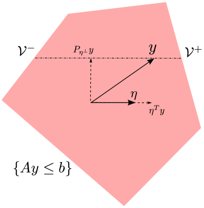
The geometric picture gives more intuition as to why ๐’ฑ+superscript๐’ฑ{\cal V}^{+} and ๐’ฑโˆ’superscript๐’ฑ{\cal V}^{-} are independent of ฮทTโ€‹ysuperscript๐œ‚๐‘‡๐‘ฆ\eta^{T}y. Without loss of generality, we assume โ€–ฮทโ€–2=1subscriptnorm๐œ‚21||\eta||_{2}=1 and yโˆผNโ€‹(ฮผ,I)similar-to๐‘ฆ๐‘๐œ‡๐ผy\sim N(\mu,I) (otherwise we could replace y๐‘ฆy by ฮฃโˆ’12โ€‹ysuperscriptฮฃ12๐‘ฆ\Sigma^{-\frac{1}{2}}y). Now we can decompose y๐‘ฆy into two independent components, a 1-dimensional component ฮทTโ€‹ysuperscript๐œ‚๐‘‡๐‘ฆ\eta^{T}y and an (nโˆ’1)๐‘›1(n-1)-dimensional component orthogonal to ฮท๐œ‚\eta:

y=ฮทTโ€‹y+PฮทโŸ‚โ€‹y.๐‘ฆsuperscript๐œ‚๐‘‡๐‘ฆsubscript๐‘ƒsuperscript๐œ‚perpendicular-to๐‘ฆy=\eta^{T}y+P_{\eta^{\perp}}y.

The case of n=2๐‘›2n=2 is illustrated in Figure 2. Since the two components are independent, the distribution of ฮทTโ€‹ysuperscript๐œ‚๐‘‡๐‘ฆ\eta^{T}y is the same as ฮทTโ€‹y|{PฮทโŸ‚โ€‹y}conditionalsuperscript๐œ‚๐‘‡๐‘ฆsubscript๐‘ƒsuperscript๐œ‚perpendicular-to๐‘ฆ\eta^{T}y|\{P_{\eta^{\perp}}y\}. If we condition on PฮทโŸ‚โ€‹ysubscript๐‘ƒsuperscript๐œ‚perpendicular-to๐‘ฆP_{\eta^{\perp}}y, it is clear from Figure 2 that in order for y๐‘ฆy to lie in the set, it is necessary for ๐’ฑโˆ’โ‰คฮทTโ€‹yโ‰ค๐’ฑ+superscript๐’ฑsuperscript๐œ‚๐‘‡๐‘ฆsuperscript๐’ฑ{\cal V}^{-}\leq\eta^{T}y\leq{\cal V}^{+}, where ๐’ฑโˆ’superscript๐’ฑ{\cal V}^{-} and ๐’ฑ+superscript๐’ฑ{\cal V}^{+} are functions of PฮทโŸ‚โ€‹ysubscript๐‘ƒsuperscript๐œ‚perpendicular-to๐‘ฆP_{\eta^{\perp}}y.

Refer to caption
Figure 2: A picture demonstrating that the set {Aโ€‹yโ‰คb}๐ด๐‘ฆ๐‘\left\{Ay\leq b\right\} can be characterized by {๐’ฑโˆ’โ‰คฮทTโ€‹yโ‰ค๐’ฑ+}superscript๐’ฑsuperscript๐œ‚๐‘‡๐‘ฆsuperscript๐’ฑ\{{\cal V}^{-}\leq\eta^{T}y\leq{\cal V}^{+}\}. Assuming ฮฃ=Iฮฃ๐ผ\Sigma=I and โ€–ฮทโ€–2=1subscriptnorm๐œ‚21||\eta||_{2}=1, ๐’ฑโˆ’superscript๐’ฑ{\cal V}^{-} and ๐’ฑ+superscript๐’ฑ{\cal V}^{+} are functions of PฮทโŸ‚โ€‹ysubscript๐‘ƒsuperscript๐œ‚perpendicular-to๐‘ฆP_{\eta^{\perp}}y only, which is independent of ฮทTโ€‹ysuperscript๐œ‚๐‘‡๐‘ฆ\eta^{T}y.
Corollary 5.2.

The distribution of ฮทTโ€‹ysuperscript๐œ‚๐‘‡๐‘ฆ\eta^{T}y conditioned on {Aโ€‹yโ‰คb,๐’ฑ+โ€‹(y)=v+,๐’ฑโˆ’โ€‹(y)=vโˆ’}formulae-sequence๐ด๐‘ฆ๐‘formulae-sequencesuperscript๐’ฑ๐‘ฆsuperscript๐‘ฃsuperscript๐’ฑ๐‘ฆsuperscript๐‘ฃ\{Ay\leq b,{\cal V}^{+}(y)=v^{+},{\cal V}^{-}(y)=v^{-}\} is a (univariate) Gaussian truncated to fall between ๐’ฑโˆ’superscript๐’ฑ{\cal V}^{-} and ๐’ฑ+superscript๐’ฑ{\cal V}^{+}, i.e.

ฮทTโ€‹yโˆฃ{Aโ€‹yโ‰คb,๐’ฑ+โ€‹(y)=v+,๐’ฑโˆ’โ€‹(y)=vโˆ’}โ€‹=๐‘‘โ€‹Wconditionalsuperscript๐œ‚๐‘‡๐‘ฆformulae-sequence๐ด๐‘ฆ๐‘formulae-sequencesuperscript๐’ฑ๐‘ฆsuperscript๐‘ฃsuperscript๐’ฑ๐‘ฆsuperscript๐‘ฃ๐‘‘๐‘Š\eta^{T}y\mid\{Ay\leq b,{\cal V}^{+}(y)=v^{+},{\cal V}^{-}(y)=v^{-}\}\overset{d}{=}W

where WโˆผTโ€‹Nโ€‹(ฮทTโ€‹ฮผ,ฮทTโ€‹ฮฃโ€‹ฮท,vโˆ’,v+)similar-to๐‘Š๐‘‡๐‘superscript๐œ‚๐‘‡๐œ‡superscript๐œ‚๐‘‡ฮฃ๐œ‚superscript๐‘ฃsuperscript๐‘ฃW\sim TN(\eta^{T}\mu,\eta^{T}\Sigma\eta,v^{-},v^{+}). Tโ€‹Nโ€‹(ฮผ,ฯƒ,a,b)๐‘‡๐‘๐œ‡๐œŽ๐‘Ž๐‘TN(\mu,\sigma,a,b) is the normal distribution truncated to lie between a๐‘Ža and b๐‘b.

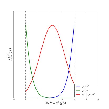
In Figure 3, we plot the density of the truncated Gaussian, noting that its shape depends on the location of ฮผ๐œ‡\mu relative to [a,b]๐‘Ž๐‘[a,b] as well as the width relative to ฯƒ๐œŽ\sigma.

Refer to caption
Figure 3: The density of the truncated Gaussian Tโ€‹Nโ€‹(ฮผ,ฯƒ2,a,b)๐‘‡๐‘๐œ‡superscript๐œŽ2๐‘Ž๐‘TN(\mu,\sigma^{2},a,b) depends on the width of [a,b]๐‘Ž๐‘[a,b] relative to ฯƒ๐œŽ\sigma as well as the location of ฮผ๐œ‡\mu relative to [a,b]๐‘Ž๐‘[a,b]. When ฮผ๐œ‡\mu is firmly inside the interval, the distribution resembles a Gaussian. As ฮผ๐œ‡\mu leaves [a,b]๐‘Ž๐‘[a,b], the density begins to converge to an exponential distribution with mean inversely proportional to the distance between ฮผ๐œ‡\mu and its projection onto [a,b]๐‘Ž๐‘[a,b].

The following pivotal quantity333The distribution of a pivotal quantity does not depend on unobserved parameters. follows from Corollary 5.2 via the probability integral transform.

Theorem 5.3.
Let ฮฆโ€‹(x)ฮฆ๐‘ฅ\Phi(x) denote the CDF of a Nโ€‹(0,1)๐‘01N(0,1) random variable, and let Fฮผ,ฯƒ2[a,b]superscriptsubscript๐น๐œ‡superscript๐œŽ2๐‘Ž๐‘F_{\mu,\sigma^{2}}^{[a,b]} denote the CDF of Tโ€‹Nโ€‹(ฮผ,ฯƒ,a,b)๐‘‡๐‘๐œ‡๐œŽ๐‘Ž๐‘TN(\mu,\sigma,a,b), i.e.:

Fฮผ,ฯƒ2[a,b]โ€‹(x)=ฮฆโ€‹((xโˆ’ฮผ)/ฯƒ)โˆ’ฮฆโ€‹((aโˆ’ฮผ)/ฯƒ)ฮฆโ€‹((bโˆ’ฮผ)/ฯƒ)โˆ’ฮฆโ€‹((aโˆ’ฮผ)/ฯƒ).superscriptsubscript๐น๐œ‡superscript๐œŽ2๐‘Ž๐‘๐‘ฅฮฆ๐‘ฅ๐œ‡๐œŽฮฆ๐‘Ž๐œ‡๐œŽฮฆ๐‘๐œ‡๐œŽฮฆ๐‘Ž๐œ‡๐œŽF_{\mu,\sigma^{2}}^{[a,b]}(x)=\frac{\Phi((x-\mu)/\sigma)-\Phi((a-\mu)/\sigma)}{\Phi((b-\mu)/\sigma)-\Phi((a-\mu)/\sigma)}. (13)

Then FฮทTโ€‹ฮผ,ฮทTโ€‹ฮฃโ€‹ฮท[๐’ฑโˆ’,๐’ฑ+]โ€‹(ฮทTโ€‹y)superscriptsubscript๐นsuperscript๐œ‚๐‘‡๐œ‡superscript๐œ‚๐‘‡ฮฃ๐œ‚superscript๐’ฑsuperscript๐’ฑsuperscript๐œ‚๐‘‡๐‘ฆF_{\eta^{T}\mu,\ \eta^{T}\Sigma\eta}^{[{\cal V}^{-},{\cal V}^{+}]}(\eta^{T}y) is a pivotal quantity, conditional on {Aโ€‹yโ‰คb}๐ด๐‘ฆ๐‘\{Ay\leq b\}:

FฮทTโ€‹ฮผ,ฮทTโ€‹ฮฃโ€‹ฮท[๐’ฑโˆ’,๐’ฑ+]โ€‹(ฮทTโ€‹y)|{Aโ€‹yโ‰คb}โˆผUnifโก(0,1)similar-toconditionalsuperscriptsubscript๐นsuperscript๐œ‚๐‘‡๐œ‡superscript๐œ‚๐‘‡ฮฃ๐œ‚superscript๐’ฑsuperscript๐’ฑsuperscript๐œ‚๐‘‡๐‘ฆ๐ด๐‘ฆ๐‘Unif01F_{\eta^{T}\mu,\ \eta^{T}\Sigma\eta}^{[{\cal V}^{-},{\cal V}^{+}]}(\eta^{T}y)\ \big{|}\ \{Ay\leq b\}\sim\operatorname{Unif}(0,1) (14)

where ๐’ฑโˆ’superscript๐’ฑ{\cal V}^{-} and ๐’ฑ+superscript๐’ฑ{\cal V}^{+} are defined in (10) and (11).

Refer to caption
Refer to caption
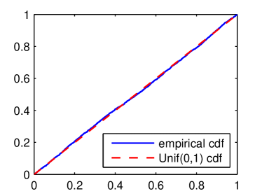
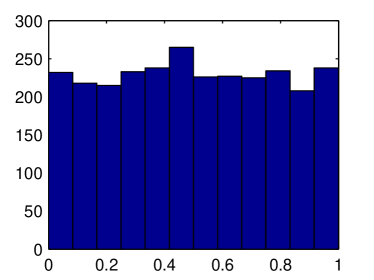
Figure 4: Histogram and qq plot of FฮทTโ€‹ฮผ,ฮทTโ€‹ฮฃโ€‹ฮท[๐’ฑโˆ’,๐’ฑ+]โ€‹(ฮทTโ€‹y)superscriptsubscript๐นsuperscript๐œ‚๐‘‡๐œ‡superscript๐œ‚๐‘‡ฮฃ๐œ‚superscript๐’ฑsuperscript๐’ฑsuperscript๐œ‚๐‘‡๐‘ฆF_{\eta^{T}\mu,\ \eta^{T}\Sigma\eta}^{[{\cal V}^{-},{\cal V}^{+}]}(\eta^{T}y) where y๐‘ฆy is a constrained Gaussian. The distribution is very close to Unifโ€‹(0,1)Unif01\text{Unif}(0,1), which is in agreement with Theorem 5.3.

6 Inference for marginal screening

In this section, we apply the theory summarized in Sections 4 and 5 to marginal screening. In particular, we will construct confidence intervals for the selected variables.

To summarize the developments so far, recall that our model (1) says that yโˆผNโ€‹(ฮผ,ฯƒ2โ€‹I)similar-to๐‘ฆ๐‘๐œ‡superscript๐œŽ2๐ผy\sim N(\mu,\sigma^{2}I). The distribution of interest is y|{E^โ€‹(y)=E}conditional๐‘ฆ^๐ธ๐‘ฆ๐ธy|\{\hat{E}(y)=E\}, and by Theorem 4.1, this is equivalent to y|{Aโ€‹(S,s)โ€‹zโ‰คbโ€‹(S,s)}conditional๐‘ฆ๐ด๐‘†๐‘ ๐‘ง๐‘๐‘†๐‘ y|{\{A(S,s)z\leq b(S,s)\}}, where yโˆผNโ€‹(ฮผ,ฯƒ2โ€‹I)similar-to๐‘ฆ๐‘๐œ‡superscript๐œŽ2๐ผy\sim N(\mu,\sigma^{2}I). By applying Theorem 5.3, we obtain the pivotal quantity

FฮทTโ€‹ฮผ,ฯƒ2โ€‹โ€–ฮทโ€–22[๐’ฑโˆ’,๐’ฑ+]โ€‹(ฮทTโ€‹y)|{E^โ€‹(y)=E}โˆผUnifโก(0,1)similar-toconditionalsuperscriptsubscript๐นsuperscript๐œ‚๐‘‡๐œ‡superscript๐œŽ2superscriptsubscriptnorm๐œ‚22superscript๐’ฑsuperscript๐’ฑsuperscript๐œ‚๐‘‡๐‘ฆ^๐ธ๐‘ฆ๐ธUnif01\displaystyle F_{\eta^{T}\mu,\ \sigma^{2}||\eta||_{2}^{2}}^{[{\cal V}^{-},{\cal V}^{+}]}(\eta^{T}y)\ \big{|}\ \{\hat{E}(y)=E\}\sim\operatorname{Unif}(0,1) (15)

for any ฮท๐œ‚\eta, where ๐’ฑโˆ’superscript๐’ฑ{\cal V}^{-} and ๐’ฑ+superscript๐’ฑ{\cal V}^{+} are defined in (10) and (11).

6.1 Hypothesis tests for selected variables

In this section, we describe how to form confidence intervals for the components of ฮฒS^โ‹†=(XS^Tโ€‹XS^)โˆ’1โ€‹XS^Tโ€‹ฮผsubscriptsuperscript๐›ฝโ‹†^๐‘†superscriptsuperscriptsubscript๐‘‹^๐‘†๐‘‡subscript๐‘‹^๐‘†1superscriptsubscript๐‘‹^๐‘†๐‘‡๐œ‡\beta^{\star}_{\hat{S}}=(X_{\hat{S}}^{T}X_{\hat{S}})^{-1}X_{\hat{S}}^{T}\mu. The best linear predictor of ฮผ๐œ‡\mu that uses only the selected variables is ฮฒS^โ‹†subscriptsuperscript๐›ฝโ‹†^๐‘†\beta^{\star}_{\hat{S}} , and ฮฒ^S^=(XS^Tโ€‹XS^)โˆ’1โ€‹XS^Tโ€‹ysubscript^๐›ฝ^๐‘†superscriptsuperscriptsubscript๐‘‹^๐‘†๐‘‡subscript๐‘‹^๐‘†1superscriptsubscript๐‘‹^๐‘†๐‘‡๐‘ฆ\hat{\beta}_{\hat{S}}=(X_{\hat{S}}^{T}X_{\hat{S}})^{-1}X_{\hat{S}}^{T}y is an unbiased estimate of ฮฒS^โ‹†subscriptsuperscript๐›ฝโ‹†^๐‘†\beta^{\star}_{\hat{S}}. In this section, we propose hypothesis tests and confidence intervals for ฮฒS^โ‹†subscriptsuperscript๐›ฝโ‹†^๐‘†\beta^{\star}_{\hat{S}}. If we choose

ฮทj=((XS^Tโ€‹XS^)โˆ’1โ€‹XS^Tโ€‹ej)T,subscript๐œ‚๐‘—superscriptsuperscriptsuperscriptsubscript๐‘‹^๐‘†๐‘‡subscript๐‘‹^๐‘†1superscriptsubscript๐‘‹^๐‘†๐‘‡subscript๐‘’๐‘—๐‘‡\eta_{j}=((X_{\hat{S}}^{T}X_{\hat{S}})^{-1}X_{\hat{S}}^{T}e_{j})^{T}, (16)

then ฮทjTโ€‹ฮผ=ฮฒjโˆˆS^โ‹†superscriptsubscript๐œ‚๐‘—๐‘‡๐œ‡superscriptsubscript๐›ฝ๐‘—^๐‘†โ‹†\eta_{j}^{T}\mu=\beta_{j\in\hat{S}}^{\star}, so the above framework provides a method for inference about the jthsuperscript๐‘—thj^{\text{th}} variable in the model S^^๐‘†\hat{S}. This choice of ฮท๐œ‚\eta is not fixed before marginal screening selects S^^๐‘†\hat{S}, but it is measurable with respect to the ฯƒ๐œŽ\sigma-algebra generated by the partition. Since it is measurable, ฮท๐œ‚\eta is constant on each partition, so the pivot is uniformly distributed on each element of the partition, and thus uniformly distributed for all y๐‘ฆy.

If we assume the linear model ฮผ=Xโ€‹ฮฒ0๐œ‡๐‘‹superscript๐›ฝ0\mu=X\beta^{0} for some ฮฒ0โˆˆ๐‘psuperscript๐›ฝ0superscript๐‘๐‘\beta^{0}\in\mathbf{R}^{p}, S0:=supportโ€‹(ฮฒ0)โŠ‚S^assignsuperscript๐‘†0supportsuperscript๐›ฝ0^๐‘†S^{0}:=\text{support}(\beta^{0})\subset\hat{S}, and XS^subscript๐‘‹^๐‘†X_{\hat{S}} is full rank, then by the following computation ฮฒS^โ‹†=ฮฒS^0subscriptsuperscript๐›ฝโ‹†^๐‘†superscriptsubscript๐›ฝ^๐‘†0\beta^{\star}_{\hat{S}}=\beta_{\hat{S}}^{0}:

ฮฒS^โ‹†subscriptsuperscript๐›ฝโ‹†^๐‘†\displaystyle\beta^{\star}_{\hat{S}} =(XS^Tโ€‹XS^)โˆ’1โ€‹XS^Tโ€‹XSโ€‹ฮฒS0absentsuperscriptsuperscriptsubscript๐‘‹^๐‘†๐‘‡subscript๐‘‹^๐‘†1superscriptsubscript๐‘‹^๐‘†๐‘‡subscript๐‘‹๐‘†superscriptsubscript๐›ฝ๐‘†0\displaystyle=(X_{\hat{S}}^{T}X_{\hat{S}})^{-1}X_{\hat{S}}^{T}X_{S}\beta_{S}^{0}
=(XS^Tโ€‹XS^)โˆ’1โ€‹XS^Tโ€‹XS^โ€‹ฮฒS^0absentsuperscriptsuperscriptsubscript๐‘‹^๐‘†๐‘‡subscript๐‘‹^๐‘†1superscriptsubscript๐‘‹^๐‘†๐‘‡subscript๐‘‹^๐‘†superscriptsubscript๐›ฝ^๐‘†0\displaystyle=(X_{\hat{S}}^{T}X_{\hat{S}})^{-1}X_{\hat{S}}^{T}X_{\hat{S}}\beta_{\hat{S}}^{0}
=ฮฒS^0absentsuperscriptsubscript๐›ฝ^๐‘†0\displaystyle=\beta_{\hat{S}}^{0}

In [9], the screening property S0โŠ‚S^superscript๐‘†0^๐‘†S^{0}\subset\hat{S} for the marginal screening algorithm is established under mild conditions. Thus under the screening property, our method provides hypothesis tests and confidence intervals for ฮฒS^0superscriptsubscript๐›ฝ^๐‘†0\beta_{\hat{S}}^{0}.

By applying Theorem 5.3, we obtain the following (conditional) pivot for ฮฒjโˆˆS^โ‹†subscriptsuperscript๐›ฝโ‹†๐‘—^๐‘†\beta^{\star}_{j\in\hat{S}}:

FฮฒjโˆˆS^โ‹†,ฯƒ2โ€‹โ€–ฮทjโ€–2[๐’ฑโˆ’,๐’ฑ+]โ€‹(ฮทjTโ€‹y)|{E^โ€‹(y)=E}โˆผUnifโก(0,1).similar-toconditionalsuperscriptsubscript๐นsubscriptsuperscript๐›ฝโ‹†๐‘—^๐‘†superscript๐œŽ2superscriptnormsubscript๐œ‚๐‘—2superscript๐’ฑsuperscript๐’ฑsuperscriptsubscript๐œ‚๐‘—๐‘‡๐‘ฆ^๐ธ๐‘ฆ๐ธUnif01\displaystyle F_{\beta^{\star}_{j\in\hat{S}},\ \sigma^{2}||\eta_{j}||^{2}}^{[{\cal V}^{-},{\cal V}^{+}]}(\eta_{j}^{T}y)\ \Big{|}\{\hat{E}(y)=E\}\sim\operatorname{Unif}(0,1). (17)

The quantities j๐‘—j and ฮทjsubscript๐œ‚๐‘—\eta_{j} are both random through E^^๐ธ\hat{E}, a quantity which is fixed after conditioning, therefore Theorem 5.3 holds even for this choice of ฮท๐œ‚\eta.

Consider testing the hypothesis H0:ฮฒjโˆˆS^โ‹†=ฮฒj:subscript๐ป0subscriptsuperscript๐›ฝโ‹†๐‘—^๐‘†subscript๐›ฝ๐‘—H_{0}:\beta^{\star}_{j\in\hat{S}}=\beta_{j}. A valid test statistic is given by Fฮฒj,ฯƒ2โ€‹โ€–ฮทjโ€–2[๐’ฑโˆ’,๐’ฑ+]โ€‹(ฮทjTโ€‹y)superscriptsubscript๐นsubscript๐›ฝ๐‘—superscript๐œŽ2superscriptnormsubscript๐œ‚๐‘—2superscript๐’ฑsuperscript๐’ฑsuperscriptsubscript๐œ‚๐‘—๐‘‡๐‘ฆF_{\beta_{j},\ \sigma^{2}||\eta_{j}||^{2}}^{[{\cal V}^{-},{\cal V}^{+}]}(\eta_{j}^{T}y), which is uniformly distributed under the null hypothesis and y|{E^โ€‹(y)=E}conditional๐‘ฆ^๐ธ๐‘ฆ๐ธy|\{\hat{E}(y)=E\}. Thus, this test would reject when Fฮฒj,ฯƒ2โ€‹โ€–ฮทjโ€–2[๐’ฑโˆ’,๐’ฑ+]โ€‹(ฮทjTโ€‹y)>1โˆ’ฮฑ2superscriptsubscript๐นsubscript๐›ฝ๐‘—superscript๐œŽ2superscriptnormsubscript๐œ‚๐‘—2superscript๐’ฑsuperscript๐’ฑsuperscriptsubscript๐œ‚๐‘—๐‘‡๐‘ฆ1๐›ผ2F_{\beta_{j},\ \sigma^{2}||\eta_{j}||^{2}}^{[{\cal V}^{-},{\cal V}^{+}]}(\eta_{j}^{T}y)>1-\frac{\alpha}{2} or Fฮฒj,ฯƒ2โ€‹โ€–ฮทjโ€–2[๐’ฑโˆ’,๐’ฑ+]โ€‹(ฮทjTโ€‹y)<ฮฑ2superscriptsubscript๐นsubscript๐›ฝ๐‘—superscript๐œŽ2superscriptnormsubscript๐œ‚๐‘—2superscript๐’ฑsuperscript๐’ฑsuperscriptsubscript๐œ‚๐‘—๐‘‡๐‘ฆ๐›ผ2F_{\beta_{j},\ \sigma^{2}||\eta_{j}||^{2}}^{[{\cal V}^{-},{\cal V}^{+}]}(\eta_{j}^{T}y)<\frac{\alpha}{2}.

Theorem 6.1.

The test of H0:ฮฒjโˆˆS^โ‹†=ฮฒj:subscript๐ป0subscriptsuperscript๐›ฝโ‹†๐‘—^๐‘†subscript๐›ฝ๐‘—H_{0}:\beta^{\star}_{j\in\hat{S}}=\beta_{j} that accepts when

ฮฑ2<Fฮฒj,ฯƒ2โ€‹โ€–ฮทjโ€–2[๐’ฑโˆ’,๐’ฑ+]โ€‹(ฮทjTโ€‹y)<1โˆ’ฮฑ2๐›ผ2superscriptsubscript๐นsubscript๐›ฝ๐‘—superscript๐œŽ2superscriptnormsubscript๐œ‚๐‘—2superscript๐’ฑsuperscript๐’ฑsuperscriptsubscript๐œ‚๐‘—๐‘‡๐‘ฆ1๐›ผ2\frac{\alpha}{2}<F_{\beta_{j},\ \sigma^{2}||\eta_{j}||^{2}}^{[{\cal V}^{-},{\cal V}^{+}]}(\eta_{j}^{T}y)<1-\frac{\alpha}{2}

is an ฮฑ๐›ผ\alpha level test of H0subscript๐ป0H_{0}.

Proof.

Under H0subscript๐ป0H_{0}, we have ฮฒjโˆˆS^โ‹†=ฮฒjsubscriptsuperscript๐›ฝโ‹†๐‘—^๐‘†subscript๐›ฝ๐‘—\beta^{\star}_{j\in\hat{S}}=\beta_{j}, so by (17) Fฮฒj,ฯƒ2โ€‹โ€–ฮทjโ€–2[๐’ฑโˆ’,๐’ฑ+]โ€‹(ฮทjTโ€‹y)|{E^โ€‹(y)=E}conditionalsuperscriptsubscript๐นsubscript๐›ฝ๐‘—superscript๐œŽ2superscriptnormsubscript๐œ‚๐‘—2superscript๐’ฑsuperscript๐’ฑsuperscriptsubscript๐œ‚๐‘—๐‘‡๐‘ฆ^๐ธ๐‘ฆ๐ธF_{\beta_{j},\ \sigma^{2}||\eta_{j}||^{2}}^{[{\cal V}^{-},{\cal V}^{+}]}(\eta_{j}^{T}y)\big{|}\{\hat{E}(y)=E\} is uniformly distributed. Thus

๐๐ซ(ฮฑ2<Fฮฒj,ฯƒ2โ€‹โ€–ฮทjโ€–2[๐’ฑโˆ’,๐’ฑ+](ฮทjTy)โ‰ค1โˆ’ฮฑ2|{E^(y)=E,H0)}=1โˆ’ฮฑ,\mathop{\mathbf{Pr}}(\frac{\alpha}{2}<F_{\beta_{j},\ \sigma^{2}||\eta_{j}||^{2}}^{[{\cal V}^{-},{\cal V}^{+}]}(\eta_{j}^{T}y)\leq 1-\frac{\alpha}{2}\big{|}\{\hat{E}(y)=E,H_{0})\}=1-\alpha,

and the type 1 error is exactly ฮฑ๐›ผ\alpha. Under H0subscript๐ป0H_{0}, but not conditional on selection event E^^๐ธ\hat{E}, we have

๐๐ซ(ฮฑ2<Fฮฒj,ฯƒ2โ€‹โ€–ฮทjโ€–2[๐’ฑโˆ’,๐’ฑ+](ฮทjTy)โ‰ค1โˆ’ฮฑ2|H0)}\displaystyle\mathop{\mathbf{Pr}}(\frac{\alpha}{2}<F_{\beta_{j},\ \sigma^{2}||\eta_{j}||^{2}}^{[{\cal V}^{-},{\cal V}^{+}]}(\eta_{j}^{T}y)\leq 1-\frac{\alpha}{2}\big{|}H_{0})\}
=โˆ‘E๐๐ซ(ฮฑ2<Fฮฒj,ฯƒ2โ€‹โ€–ฮทjโ€–2[๐’ฑโˆ’,๐’ฑ+](ฮทjTy)โ‰ค1โˆ’ฮฑ2|{E^(y)=E,H0)}๐๐ซ(E^(y)=E|H0)\displaystyle=\sum_{E}\mathop{\mathbf{Pr}}(\frac{\alpha}{2}<F_{\beta_{j},\ \sigma^{2}||\eta_{j}||^{2}}^{[{\cal V}^{-},{\cal V}^{+}]}(\eta_{j}^{T}y)\leq 1-\frac{\alpha}{2}\big{|}\{\hat{E}(y)=E,H_{0})\}\mathop{\mathbf{Pr}}(\hat{E}(y)=E|H_{0})
=โˆ‘E(1โˆ’ฮฑ)โ€‹๐๐ซ(E^โ€‹(y)=E|H0)absentsubscript๐ธ1๐›ผ๐๐ซ^๐ธ๐‘ฆconditional๐ธsubscript๐ป0\displaystyle=\sum_{E}(1-\alpha)\mathop{\mathbf{Pr}}(\hat{E}(y)=E|H_{0})
=(1โˆ’ฮฑ)โ€‹โˆ‘E๐๐ซ(E^โ€‹(y)=E|H0)absent1๐›ผsubscript๐ธ๐๐ซ^๐ธ๐‘ฆconditional๐ธsubscript๐ป0\displaystyle=(1-\alpha)\sum_{E}\mathop{\mathbf{Pr}}(\hat{E}(y)=E|H_{0})
=1โˆ’ฮฑ.absent1๐›ผ\displaystyle=1-\alpha.

For each element of the partition E๐ธE, the conditional (on selection) hypothesis test is level 1โˆ’ฮฑ1๐›ผ1-\alpha, so by summing over the partition the unconditional test is level 1โˆ’ฮฑ1๐›ผ1-\alpha. โˆŽ

Our hypothesis test is not conservative, in the sense that the type 1 error is exactly ฮฑ๐›ผ\alpha; also, it is non-asymptotic, since the statement holds for fixed n๐‘›n and p๐‘p. We summarize the hypothesis test in this section in the following algorithm.

Algorithm 2 Hypothesis test for selected variables
1:Input: Design matrix X๐‘‹X, response y๐‘ฆy, model size k๐‘˜k.
2:Use Algorithm 1 to select a subset of variables S^^๐‘†\hat{S} and signs s^=signโ€‹(XS^Tโ€‹y)^๐‘ signsuperscriptsubscript๐‘‹^๐‘†๐‘‡๐‘ฆ\hat{s}=\text{sign}(X_{\hat{S}}^{T}y).
3:Specify the null hypothesis H0:ฮฒjโˆˆS^โ‹†=ฮฒj:subscript๐ป0subscriptsuperscript๐›ฝโ‹†๐‘—^๐‘†subscript๐›ฝ๐‘—H_{0}:\beta^{\star}_{j\in\hat{S}}=\beta_{j}.
4:Let A=Aโ€‹(S^,s^)๐ด๐ด^๐‘†^๐‘ A=A(\hat{S},\hat{s}) and b=bโ€‹(S^,s^)๐‘๐‘^๐‘†^๐‘ b=b(\hat{S},\hat{s}) using (7). Let ฮทj=(XS^T)โ€ โ€‹ejsubscript๐œ‚๐‘—superscriptsuperscriptsubscript๐‘‹^๐‘†๐‘‡โ€ subscript๐‘’๐‘—\eta_{j}=(X_{\hat{S}}^{T})^{\dagger}e_{j}.
5:Compute Fฮฒj,ฯƒ2โ€‹โ€–ฮทjโ€–2[๐’ฑโˆ’,๐’ฑ+]โ€‹(ฮทjTโ€‹y)superscriptsubscript๐นsubscript๐›ฝ๐‘—superscript๐œŽ2superscriptnormsubscript๐œ‚๐‘—2superscript๐’ฑsuperscript๐’ฑsuperscriptsubscript๐œ‚๐‘—๐‘‡๐‘ฆF_{\beta_{j},\ \sigma^{2}||\eta_{j}||^{2}}^{[{\cal V}^{-},{\cal V}^{+}]}(\eta_{j}^{T}y), where ๐’ฑโˆ’superscript๐’ฑ{\cal V}^{-} and ๐’ฑ+superscript๐’ฑ{\cal V}^{+} are computed via (10) and (11) using the A๐ดA, b๐‘b, and ฮท๐œ‚\eta previously defined.
6:Output: Reject if Fฮฒj,ฯƒ2โ€‹โ€–ฮทjโ€–2[๐’ฑโˆ’,๐’ฑ+]โ€‹(ฮทjTโ€‹y)>ฮฑ2superscriptsubscript๐นsubscript๐›ฝ๐‘—superscript๐œŽ2superscriptnormsubscript๐œ‚๐‘—2superscript๐’ฑsuperscript๐’ฑsuperscriptsubscript๐œ‚๐‘—๐‘‡๐‘ฆ๐›ผ2F_{\beta_{j},\ \sigma^{2}||\eta_{j}||^{2}}^{[{\cal V}^{-},{\cal V}^{+}]}(\eta_{j}^{T}y)>\frac{\alpha}{2} or Fฮฒj,ฯƒ2โ€‹โ€–ฮทjโ€–2[๐’ฑโˆ’,๐’ฑ+]โ€‹(ฮทjTโ€‹y)<1โˆ’ฮฑ2superscriptsubscript๐นsubscript๐›ฝ๐‘—superscript๐œŽ2superscriptnormsubscript๐œ‚๐‘—2superscript๐’ฑsuperscript๐’ฑsuperscriptsubscript๐œ‚๐‘—๐‘‡๐‘ฆ1๐›ผ2F_{\beta_{j},\ \sigma^{2}||\eta_{j}||^{2}}^{[{\cal V}^{-},{\cal V}^{+}]}(\eta_{j}^{T}y)<1-\frac{\alpha}{2}.

6.2 Confidence intervals for selected variables

Next, we discuss how to obtain confidence intervals for ฮฒjโˆˆS^โ‹†subscriptsuperscript๐›ฝโ‹†๐‘—^๐‘†\beta^{\star}_{j\in\hat{S}}. The standard way to obtain an interval is to invert a pivotal quantity [4]. In other words, since

๐๐ซ(ฮฑ2โ‰คFฮฒjโˆˆS^โ‹†,ฯƒ2โ€‹โ€–ฮทjโ€–2[๐’ฑโˆ’,๐’ฑ+]โ€‹(ฮทjTโ€‹y)โ‰ค1โˆ’ฮฑ2|{E^=E})=ฮฑ,๐๐ซ๐›ผ2superscriptsubscript๐นsubscriptsuperscript๐›ฝโ‹†๐‘—^๐‘†superscript๐œŽ2superscriptnormsubscript๐œ‚๐‘—2superscript๐’ฑsuperscript๐’ฑsuperscriptsubscript๐œ‚๐‘—๐‘‡๐‘ฆ1conditional๐›ผ2^๐ธ๐ธ๐›ผ\mathop{\mathbf{Pr}}\left(\frac{\alpha}{2}\leq F_{\beta^{\star}_{j\in\hat{S}},\ \sigma^{2}||\eta_{j}||^{2}}^{[{\cal V}^{-},{\cal V}^{+}]}(\eta_{j}^{T}y)\leq 1-\frac{\alpha}{2}\ \big{|}\ \{\hat{E}=E\}\right)=\alpha,

one can define a (1โˆ’ฮฑ)1๐›ผ(1-\alpha) (conditional) confidence interval for ฮฒj,E^โ‹†superscriptsubscript๐›ฝ๐‘—^๐ธโ‹†\beta_{j,\hat{E}}^{\star} as

{x:ฮฑ2โ‰คFx,ฯƒ2โ€‹โ€–ฮทjโ€–2[๐’ฑโˆ’,๐’ฑ+]โ€‹(ฮทjTโ€‹y)โ‰ค1โˆ’ฮฑ2}.conditional-set๐‘ฅ๐›ผ2superscriptsubscript๐น๐‘ฅsuperscript๐œŽ2superscriptnormsubscript๐œ‚๐‘—2superscript๐’ฑsuperscript๐’ฑsuperscriptsubscript๐œ‚๐‘—๐‘‡๐‘ฆ1๐›ผ2\displaystyle\left\{x:\frac{\alpha}{2}\leq F_{x,\ \sigma^{2}||\eta_{j}||^{2}}^{[{\cal V}^{-},{\cal V}^{+}]}(\eta_{j}^{T}y)\leq 1-\frac{\alpha}{2}\right\}. (18)

In fact, F๐นF is monotone decreasing in x๐‘ฅx, so to find its endpoints, one need only solve for the root of a smooth one-dimensional function. The monotonicity is a consequence of the fact that the truncated Gaussian distribution is a natural exponential family and hence has monotone likelihood ratio in ฮผ๐œ‡\mu [21].

We now formalize the above observations in the following result, an immediate consequence of Theorem 5.3.

Corollary 6.2.

Let ฮทjsubscript๐œ‚๐‘—\eta_{j} be defined as in (16), and let Lฮฑ=Lฮฑโ€‹(ฮทj,(S^,s^))subscript๐ฟ๐›ผsubscript๐ฟ๐›ผsubscript๐œ‚๐‘—^๐‘†^๐‘ L_{\alpha}=L_{\alpha}(\eta_{j},(\hat{S},\hat{s})) and Uฮฑ=Uฮฑโ€‹(ฮทj,(S^,s^))subscript๐‘ˆ๐›ผsubscript๐‘ˆ๐›ผsubscript๐œ‚๐‘—^๐‘†^๐‘ U_{\alpha}=U_{\alpha}(\eta_{j},(\hat{S},\hat{s})) be the (unique) values satisfying

FLฮฑ,ฯƒ2โ€‹โ€–ฮทjโ€–2[๐’ฑโˆ’,๐’ฑ+]โ€‹(ฮทjTโ€‹y)superscriptsubscript๐นsubscript๐ฟ๐›ผsuperscript๐œŽ2superscriptnormsubscript๐œ‚๐‘—2superscript๐’ฑsuperscript๐’ฑsuperscriptsubscript๐œ‚๐‘—๐‘‡๐‘ฆ\displaystyle F_{L_{\alpha},\ \sigma^{2}||\eta_{j}||^{2}}^{[{\cal V}^{-},{\cal V}^{+}]}(\eta_{j}^{T}y) =1โˆ’ฮฑ2absent1๐›ผ2\displaystyle=1-\frac{\alpha}{2} FUฮฑ,ฯƒ2โ€‹โ€–ฮทjโ€–2[๐’ฑโˆ’,๐’ฑ+]โ€‹(ฮทjTโ€‹y)superscriptsubscript๐นsubscript๐‘ˆ๐›ผsuperscript๐œŽ2superscriptnormsubscript๐œ‚๐‘—2superscript๐’ฑsuperscript๐’ฑsuperscriptsubscript๐œ‚๐‘—๐‘‡๐‘ฆ\displaystyle F_{U_{\alpha},\ \sigma^{2}||\eta_{j}||^{2}}^{[{\cal V}^{-},{\cal V}^{+}]}(\eta_{j}^{T}y) =ฮฑ2absent๐›ผ2\displaystyle=\frac{\alpha}{2} (19)

Then [Lฮฑ,Uฮฑ]subscript๐ฟ๐›ผsubscript๐‘ˆ๐›ผ[L_{\alpha},U_{\alpha}] is a (1โˆ’ฮฑ)1๐›ผ(1-\alpha) confidence interval for ฮฒjโˆˆS^โ‹†subscriptsuperscript๐›ฝโ‹†๐‘—^๐‘†\beta^{\star}_{j\in\hat{S}}, conditional on E^^๐ธ\hat{E}:

โ„™โ€‹(ฮฒjโˆˆS^โ‹†โˆˆ[Lฮฑ,Uฮฑ]|{E^=E})=1โˆ’ฮฑ.โ„™subscriptsuperscript๐›ฝโ‹†๐‘—^๐‘†conditionalsubscript๐ฟ๐›ผsubscript๐‘ˆ๐›ผ^๐ธ๐ธ1๐›ผ\mathbb{P}\left(\beta^{\star}_{j\in\hat{S}}\in[L_{\alpha},U_{\alpha}]\ \big{|}\ \{\hat{E}=E\}\right)=1-\alpha. (20)
Proof.

The confidence region of ฮฒjโˆˆS^โ‹†subscriptsuperscript๐›ฝโ‹†๐‘—^๐‘†\beta^{\star}_{j\in\hat{S}} is the set of ฮฒjsubscript๐›ฝ๐‘—\beta_{j} such that the test of H0:ฮฒjโˆˆS^โ‹†:subscript๐ป0subscriptsuperscript๐›ฝโ‹†๐‘—^๐‘†H_{0}:\beta^{\star}_{j\in\hat{S}} accepts at the 1โˆ’ฮฑ1๐›ผ1-\alpha level. The function Fx,ฯƒ2โ€‹โ€–ฮทjโ€–2[๐’ฑโˆ’,๐’ฑ+]โ€‹(ฮทjTโ€‹y)superscriptsubscript๐น๐‘ฅsuperscript๐œŽ2superscriptnormsubscript๐œ‚๐‘—2superscript๐’ฑsuperscript๐’ฑsuperscriptsubscript๐œ‚๐‘—๐‘‡๐‘ฆF_{x,\ \sigma^{2}||\eta_{j}||^{2}}^{[{\cal V}^{-},{\cal V}^{+}]}(\eta_{j}^{T}y) is monotone in x๐‘ฅx, so solving for Lฮฑsubscript๐ฟ๐›ผL_{\alpha} and Uฮฑsubscript๐‘ˆ๐›ผU_{\alpha} identify the most extreme values where H0subscript๐ป0H_{0} is still accepted. This gives a 1โˆ’ฮฑ1๐›ผ1-\alpha confidence interval. โˆŽ

In relation to the literature on False Coverage Rate (FCR) [1], our procedure also controls the FCR.

Lemma 6.3.

For each jโˆˆS^๐‘—^๐‘†j\in\hat{S},

๐๐ซ(ฮฒjโˆˆS^โ‹†โˆˆ[Lฮฑj,Uฮฑj])=1โˆ’ฮฑ.๐๐ซsubscriptsuperscript๐›ฝโ‹†๐‘—^๐‘†superscriptsubscript๐ฟ๐›ผ๐‘—superscriptsubscript๐‘ˆ๐›ผ๐‘—1๐›ผ\mathop{\mathbf{Pr}}\left(\beta^{\star}_{j\in\hat{S}}\in[L_{\alpha}^{j},U_{\alpha}^{j}]\right)=1-\alpha. (21)

Furthermore, the FCR of the intervals {[Lฮฑj,Uฮฑj]}jโˆˆE^subscriptsuperscriptsubscript๐ฟ๐›ผ๐‘—superscriptsubscript๐‘ˆ๐›ผ๐‘—๐‘—^๐ธ\left\{[L_{\alpha}^{j},U_{\alpha}^{j}]\right\}_{j\in\hat{E}} is ฮฑ๐›ผ\alpha.

Proof.

By (20), the conditional coverage of the confidence intervals are 1โˆ’ฮฑ1๐›ผ1-\alpha. The coverage holds for every element of the partition {E^โ€‹(y)=E}^๐ธ๐‘ฆ๐ธ\{\hat{E}(y)=E\}, so

๐๐ซ(ฮฒjโˆˆS^โ‹†โˆˆ[Lฮฑj,Uฮฑj])๐๐ซsubscriptsuperscript๐›ฝโ‹†๐‘—^๐‘†superscriptsubscript๐ฟ๐›ผ๐‘—superscriptsubscript๐‘ˆ๐›ผ๐‘—\displaystyle\mathop{\mathbf{Pr}}\left(\beta^{\star}_{j\in\hat{S}}\in[L_{\alpha}^{j},U_{\alpha}^{j}]\right)
=โˆ‘E๐๐ซ(ฮฒjโˆˆS^โ‹†โˆˆ[Lฮฑ,Uฮฑ]|{E^=E})โ€‹๐๐ซ(E^=E)absentsubscript๐ธ๐๐ซsubscriptsuperscript๐›ฝโ‹†๐‘—^๐‘†conditionalsubscript๐ฟ๐›ผsubscript๐‘ˆ๐›ผ^๐ธ๐ธ๐๐ซ^๐ธ๐ธ\displaystyle=\sum_{E}\mathop{\mathbf{Pr}}\left(\beta^{\star}_{j\in\hat{S}}\in[L_{\alpha},U_{\alpha}]\ \big{|}\ \{\hat{E}=E\}\right)\mathop{\mathbf{Pr}}(\hat{E}=E)
=โˆ‘E(1โˆ’ฮฑ)โ€‹๐๐ซ(E^=E)absentsubscript๐ธ1๐›ผ๐๐ซ^๐ธ๐ธ\displaystyle=\sum_{E}(1-\alpha)\mathop{\mathbf{Pr}}(\hat{E}=E)
=(1โˆ’ฮฑ)โ€‹โˆ‘E๐๐ซ(E^=E)absent1๐›ผsubscript๐ธ๐๐ซ^๐ธ๐ธ\displaystyle=(1-\alpha)\sum_{E}\mathop{\mathbf{Pr}}(\hat{E}=E)
=1โˆ’ฮฑ.absent1๐›ผ\displaystyle=1-\alpha.

โˆŽ

Refer to caption
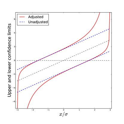
Figure 5: Comparison of adjusted and unadjusted 90% confidence interval for Tโ€‹Nโ€‹(ฮผ,ฯƒ2,a,b)๐‘‡๐‘๐œ‡superscript๐œŽ2๐‘Ž๐‘TN(\mu,\sigma^{2},a,b). The upper and lower bounds of 90% confidence intervals are based on [a,b]=[โˆ’3โ€‹ฯƒ,3โ€‹ฯƒ]๐‘Ž๐‘3๐œŽ3๐œŽ[a,b]=[-3\sigma,3\sigma], and the x-axis plots the observation on the scale xฯƒ๐‘ฅ๐œŽ\frac{x}{\sigma}. We see that as long as the obser vation xฯƒ๐‘ฅ๐œŽ\frac{x}{\sigma} is roughly 0.5โ€‹ฯƒ0.5๐œŽ0.5\sigma away from either boundary, the size of the intervals is comparable to an unadjusted confidence interval. However, the adjusted intervals are guaranteed to have the correct coverage, whereas it is unknown when the unadjusted intervals have the correct coverage.

We summarize the algorithm for selecting and constructing confidence intervals below.

Algorithm 3 Confidence intervals for selected variables
1:Input: Design matrix X๐‘‹X, response y๐‘ฆy, model size k๐‘˜k.
2:Use Algorithm 1 to select a subset of variables S^^๐‘†\hat{S} and signs s^=signโ€‹(XS^Tโ€‹y)^๐‘ signsuperscriptsubscript๐‘‹^๐‘†๐‘‡๐‘ฆ\hat{s}=\text{sign}(X_{\hat{S}}^{T}y).
3:Let A=Aโ€‹(S^,s^)๐ด๐ด^๐‘†^๐‘ A=A(\hat{S},\hat{s}) and b=bโ€‹(S^,s^)๐‘๐‘^๐‘†^๐‘ b=b(\hat{S},\hat{s}) using (7). Let ฮทj=(XS^T)โ€ โ€‹ejsubscript๐œ‚๐‘—superscriptsuperscriptsubscript๐‘‹^๐‘†๐‘‡โ€ subscript๐‘’๐‘—\eta_{j}=(X_{\hat{S}}^{T})^{\dagger}e_{j}.
4:Solve for Lฮฑjsubscriptsuperscript๐ฟ๐‘—๐›ผL^{j}_{\alpha} and Uฮฑjsubscriptsuperscript๐‘ˆ๐‘—๐›ผU^{j}_{\alpha} using Equation (19) where ๐’ฑโˆ’superscript๐’ฑ{\cal V}^{-} and ๐’ฑ+superscript๐’ฑ{\cal V}^{+} are computed via (10) and (11) using the A๐ดA, b๐‘b, and ฮทjsubscript๐œ‚๐‘—\eta_{j} previously defined.
5:Output: Return the intervals [Lฮฑj,Uฮฑj]subscriptsuperscript๐ฟ๐‘—๐›ผsubscriptsuperscript๐‘ˆ๐‘—๐›ผ[L^{j}_{\alpha},U^{j}_{\alpha}] for jโˆˆS^๐‘—^๐‘†j\in\hat{S}.

6.3 Experiments on Diabetes dataset

Refer to caption
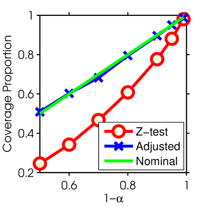
Figure 6: Plot of 1โˆ’ฮฑ1๐›ผ1-\alpha vs the coverage proportion for diabetes dataset. The nominal curve is the line y=x๐‘ฆ๐‘ฅy=x. The coverage proportion of the adjusted intervals agree with the nominal coverage level, but the z-test coverage proportion is strictly below the nominal level. The adjusted intervals perform well, despite the noise being non-Gaussian, and ฯƒ2superscript๐œŽ2\sigma^{2} unknown.

In Figure 1, we have already seen that the confidence intervals constructed using Algorithm 3 have exactly 1โˆ’ฮฑ1๐›ผ1-\alpha coverage proportion. In this section, we perform an experiment on real data where the linear model does not hold, the noise is not Gaussian, and the noise variance is unknown. The diabetes dataset contains n=442๐‘›442n=442 diabetes patients measured on p=10๐‘10p=10 baseline variables [6]. The baseline variables are age, sex, body mass index, average blood pressure, and six blood serum measurements, and the response y๐‘ฆy is a quantitative measure of disease progression measured one year after the baseline. The goal is to use the baseline variables to predict y๐‘ฆy, the measure of disease progression after one year, and determine which baseline variables are statistically significant for predicting y๐‘ฆy.

Since the noise variance ฯƒ2superscript๐œŽ2\sigma^{2} is unknown, we estimate it by ฯƒ2=โ€–yโˆ’y^โ€–nโˆ’psuperscript๐œŽ2norm๐‘ฆ^๐‘ฆ๐‘›๐‘\sigma^{2}=\frac{\left\|y-\hat{y}\right\|}{n-p}, where y^=Xโ€‹ฮฒ^^๐‘ฆ๐‘‹^๐›ฝ\hat{y}=X\hat{\beta} and ฮฒ^=(XTโ€‹X)โˆ’1โ€‹XTโ€‹y^๐›ฝsuperscriptsuperscript๐‘‹๐‘‡๐‘‹1superscript๐‘‹๐‘‡๐‘ฆ\hat{\beta}=(X^{T}X)^{-1}X^{T}y. For each trial we generated new responses y~i=Xโ€‹ฮฒ^+ฯต~subscript~๐‘ฆ๐‘–๐‘‹^๐›ฝ~italic-ฯต\tilde{y}_{i}=X\hat{\beta}+\tilde{\epsilon}, and ฯต~~italic-ฯต\tilde{\epsilon} is bootstrapped from the residuals ri=yiโˆ’y^isubscript๐‘Ÿ๐‘–subscript๐‘ฆ๐‘–subscript^๐‘ฆ๐‘–r_{i}=y_{i}-\hat{y}_{i}. This is known as the residual bootstrap, and is a standard method for assessing statistical procedures when the underlying model is unknown [7]. We used marginal screening to select k=2๐‘˜2k=2 variables, and then fit linear regression on the selected variables. The adjusted confidence intervals were constructed using Algorithm 3 with the estimated ฯƒ2superscript๐œŽ2\sigma^{2}. The nominal coverage level is varied across 1โˆ’ฮฑโˆˆ{.5,.6,.7,.8,.9,.95,.99}1๐›ผ.5.6.7.8.9.95.991-\alpha\in\{.5,.6,.7,.8,.9,.95,.99\}. From Figure 6, we observe that the adjusted intervals always cover at the nominal level, whereas the z-test is always below. The experiment was repeated 200020002000 times.

7 Extensions

The purpose of this section is to illustrate the broad applicability of the condition on selection framework. This framework was first proposed in [16] to form valid hypothesis tests and confidence intervals after model selection via the Lasso. However, the framework is not restricted to the Lasso, and we have shown how to apply it to marginal screening. For expository purposes, we focused the paper on marginal screening where the framework is particularly easy to understand. In the rest of this section, we show how to apply the framework to marginal screening+Lasso, orthogonal matching pursuit, and non-negative least squares. This is a non-exhaustive list of selection procedures where the condition on selection framework is applicable, but we hope this incomplete list emphasizes the ease of constructing tests and confidence intervals post-model selection via conditioning.

7.1 Marginal screening + Lasso

The marginal screening+Lasso procedure was introduced in [9] as a variable selection method for the ultra-high dimensional setting of p=Oโ€‹(enk)๐‘๐‘‚superscript๐‘’superscript๐‘›๐‘˜p=O(e^{n^{k}}). Fan et al. [9] recommend applying the marginal screening algorithm with k=nโˆ’1๐‘˜๐‘›1k=n-1, followed by the Lasso on the selected variables. This is a two-stage procedure, so to properly account for the selection we must encode the selection event of marginal screening followed by Lasso. This can be done by representing the two stage selection as a single event. Let (S^m,s^m)subscript^๐‘†๐‘šsubscript^๐‘ ๐‘š(\hat{S}_{m},\hat{s}_{m}) be the variables and signs selected by marginal screening, and the (S^L,z^L)subscript^๐‘†๐ฟsubscript^๐‘ง๐ฟ(\hat{S}_{L},\hat{z}_{L}) be the variables and signs selected by Lasso [16]. In Proposition 2.2 of [16], it is shown how to encode the Lasso selection event (S^L,z^L)subscript^๐‘†๐ฟsubscript^๐‘ง๐ฟ(\hat{S}_{L},\hat{z}_{L}) as a set of constraints {ALโ€‹yโ‰คbL}subscript๐ด๐ฟ๐‘ฆsubscript๐‘๐ฟ\{A_{L}y\leq b_{L}\} 444The Lasso selection event is with respect to the Lasso optimization problem after marginal screening., and in Section 4 we showed how to encode the marginal screening selection event (S^m,s^m)subscript^๐‘†๐‘šsubscript^๐‘ ๐‘š(\hat{S}_{m},\hat{s}_{m}) as a set of constraints {Amโ€‹yโ‰คbm}subscript๐ด๐‘š๐‘ฆsubscript๐‘๐‘š\{A_{m}y\leq b_{m}\}. Thus the selection event of marginal screening+Lasso can be encoded as {ALโ€‹yโ‰คbL,Amโ€‹yโ‰คbm}formulae-sequencesubscript๐ด๐ฟ๐‘ฆsubscript๐‘๐ฟsubscript๐ด๐‘š๐‘ฆsubscript๐‘๐‘š\{A_{L}y\leq b_{L},A_{m}y\leq b_{m}\}. Using these constraints, the hypothesis test and confidence intervals described in Algorithms 2 and 3 are valid for marginal screening+Lasso.

7.2 Orthogonal Matching Pursuit

Orthogonal matching pursuit (OMP) is a commonly used variable selection method. At each iteration, OMP selects the variable most correlated with the residual r๐‘Ÿr, and then recomputes the residual using the residual of least squares using the selected variables. The description of the OMP algorithm is given in Algorithm 4.

Algorithm 4 Orthogonal matching pursuit (OMP)
1:Input: Design matrix X๐‘‹X, response y๐‘ฆy, and model size k๐‘˜k.
2:for: i=1๐‘–1i=1 to k๐‘˜k
3:โ€ƒpi=argโกmaxj=1,โ€ฆ,pโก|riTโ€‹xj|subscript๐‘๐‘–subscript๐‘—1โ€ฆ๐‘superscriptsubscript๐‘Ÿ๐‘–๐‘‡subscript๐‘ฅ๐‘—p_{i}=\arg\max_{j=1,\ldots,p}|r_{i}^{T}x_{j}|.
4:โ€ƒS^i=โˆชj=1i{pi}subscript^๐‘†๐‘–superscriptsubscript๐‘—1๐‘–subscript๐‘๐‘–\hat{S}_{i}=\cup_{j=1}^{i}\ \{p_{i}\}.
5:โ€ƒri+1=(Iโˆ’XS^iโ€‹XS^iโ€ )โ€‹ysubscript๐‘Ÿ๐‘–1๐ผsubscript๐‘‹subscript^๐‘†๐‘–superscriptsubscript๐‘‹subscript^๐‘†๐‘–โ€ ๐‘ฆr_{i+1}=(I-X_{\hat{S}_{i}}X_{\hat{S}_{i}}^{\dagger})y.
6:end for
7:Output: S^:={p1,โ€ฆ,pk}assign^๐‘†subscript๐‘1โ€ฆsubscript๐‘๐‘˜\hat{S}:=\{p_{1},\ldots,p_{k}\}, and ฮฒ^S^=(XS^Tโ€‹XS^)โˆ’1โ€‹XS^Tโ€‹ysubscript^๐›ฝ^๐‘†superscriptsuperscriptsubscript๐‘‹^๐‘†๐‘‡subscript๐‘‹^๐‘†1superscriptsubscript๐‘‹^๐‘†๐‘‡๐‘ฆ\hat{\beta}_{\hat{S}}=(X_{\hat{S}}^{T}X_{\hat{S}})^{-1}X_{\hat{S}}^{T}y

Similar to Section 4, we can represent the OMP selection event as a set of linear constraints on y๐‘ฆy.

E^โ€‹(y)^๐ธ๐‘ฆ\displaystyle\hat{E}(y) ={y:signโ€‹(xpiTโ€‹ri)โ€‹xpiTโ€‹ri>ยฑxjTโ€‹riโ€‹, for allย โ€‹jโ‰ piโ€‹ย and allย iโˆˆ[k]}absentconditional-set๐‘ฆsignsuperscriptsubscript๐‘ฅsubscript๐‘๐‘–๐‘‡subscript๐‘Ÿ๐‘–superscriptsubscript๐‘ฅsubscript๐‘๐‘–๐‘‡subscript๐‘Ÿ๐‘–plus-or-minussuperscriptsubscript๐‘ฅ๐‘—๐‘‡subscript๐‘Ÿ๐‘–, for allย ๐‘—subscript๐‘๐‘–ย and allย iโˆˆ[k]\displaystyle=\left\{y:\text{sign}(x_{p_{i}}^{T}r_{i})x_{p_{i}}^{T}r_{i}>\pm x_{j}^{T}r_{i}\text{, for all }j\neq p_{i}\text{ and all $i\in[k]$}\right\}
={y:s^ixpiT(Iโˆ’XS^iโˆ’1XS^iโˆ’1โ€ )y>ยฑxjT(Iโˆ’XS^iโˆ’1XS^iโˆ’1โ€ )yย and\displaystyle=\{y:\hat{s}_{i}x_{p_{i}}^{T}(I-X_{\hat{S}_{i-1}}X_{\hat{S}_{i-1}}^{\dagger})y>\pm x_{j}^{T}(I-X_{\hat{S}_{i-1}}X_{\hat{S}_{i-1}}^{\dagger})y\text{ and }
s^ixpiT(Iโˆ’XS^iโˆ’1XS^iโˆ’1โ€ )y>0, for allย jโ‰ pi, and allย iโˆˆ[k]ย }\displaystyle\hat{s}_{i}x_{p_{i}}^{T}(I-X_{\hat{S}_{i-1}}X_{\hat{S}_{i-1}}^{\dagger})y>0\text{, for all }j\neq p_{i}\text{, and all $i\in[k]$ }\}
={y:Aโ€‹(S^1,โ€ฆ,S^k,s^1,โ€ฆ,s^k)โ‰คbโ€‹(S^1,โ€ฆ,S^k,s^1,โ€ฆ,s^k)}.absentconditional-set๐‘ฆ๐ดsubscript^๐‘†1โ€ฆsubscript^๐‘†๐‘˜subscript^๐‘ 1โ€ฆsubscript^๐‘ ๐‘˜๐‘subscript^๐‘†1โ€ฆsubscript^๐‘†๐‘˜subscript^๐‘ 1โ€ฆsubscript^๐‘ ๐‘˜\displaystyle=\left\{y:A(\hat{S}_{1},\ldots,\hat{S}_{k},\hat{s}_{1},\ldots,\hat{s}_{k})\leq b(\hat{S}_{1},\ldots,\hat{S}_{k},\hat{s}_{1},\ldots,\hat{s}_{k})\right\}.

The selection event encodes that OMP selected a certain variable and the sign of the correlation of that variable with the residual, at steps 111 to k๐‘˜k. The primary difference between the OMP selection event and the marginal screening selection event is that the OMP event also describes the order at which the variables were chosen. The marginal screening event only describes that the variable was among the top k๐‘˜k most correlated, and not whether a variable was the most correlated or kโ€‹tโ€‹h๐‘˜๐‘กโ„Žkth most correlated.

Since the selection event can be represented as constraints on y๐‘ฆy, the hypothesis test and confidence intervals described in Algorithms 2 and 3 are valid for OMP selected ฮฒ^S^subscript^๐›ฝ^๐‘†\hat{\beta}_{\hat{S}}.

7.3 Nonnegative Least Squares

Non-negative least squares (NNLS) is a simple modification of the linear regression estimator with non-negative constraints on ฮฒ๐›ฝ\beta:

argโกminฮฒ:ฮฒโ‰ฅ0โก12โ€‹โ€–yโˆ’Xโ€‹ฮฒโ€–2.subscript:๐›ฝ๐›ฝ012superscriptnorm๐‘ฆ๐‘‹๐›ฝ2\displaystyle\arg\min_{\beta:\beta\geq 0}\frac{1}{2}\left\|y-X\beta\right\|^{2}. (22)

Under a positive eigenvalue conditions on X๐‘‹X, several authors [26, 22] have shown that NNLS is comprable to the Lasso in terms of prediction and estimation errors. The NNLS estimator also does not have any tuning parameters, since the sign constraint provides a natural form of regularization. NNLS has found applications when modeling non-negative data such as prices, incomes, count data. Non-negativity constraints arise naturally in non-negative matrix factorization, signal deconvolution, spectral analysis, and network tomography; we refer to [5] for a comprehensive survey of the applications of NNLS.

We show how our framework can be used to form exact hypothesis tests and confidence intervals for NNLS estimated coefficients. The primal dual solution pair (ฮฒ^,ฮป^)^๐›ฝ^๐œ†(\hat{\beta},\hat{\lambda}) is a solution iff the KKT conditions are satisfied,

ฮป^i:=โˆ’xiTโ€‹(yโˆ’Xโ€‹ฮฒ^)assignsubscript^๐œ†๐‘–superscriptsubscript๐‘ฅ๐‘–๐‘‡๐‘ฆ๐‘‹^๐›ฝ\displaystyle\hat{\lambda}_{i}:=-x_{i}^{T}(y-X\hat{\beta}) โ‰ฅ0โ€‹ย for all iabsent0ย for all i\displaystyle\geq 0\text{ for all i}
ฮฒ^^๐›ฝ\displaystyle\hat{\beta} โ‰ฅ0.absent0\displaystyle\geq 0.

Let S^={i:โˆ’xiTโ€‹(yโˆ’Xโ€‹ฮฒ^)=0}^๐‘†conditional-set๐‘–superscriptsubscript๐‘ฅ๐‘–๐‘‡๐‘ฆ๐‘‹^๐›ฝ0\hat{S}=\{i:-x_{i}^{T}(y-X\hat{\beta})=0\}. By complementary slackness ฮฒ^โˆ’S^=0subscript^๐›ฝ^๐‘†0\hat{\beta}_{-\hat{S}}=0, where โˆ’S^^๐‘†-\hat{S} is the complement to the โ€œactiveโ€ variables S^^๐‘†\hat{S} chosen by NNLS. Given the active set we can solve the KKT equation for the value of ฮฒ^S^subscript^๐›ฝ^๐‘†\hat{\beta}_{\hat{S}},

โˆ’XS^Tโ€‹(yโˆ’Xโ€‹ฮฒ^)=0superscriptsubscript๐‘‹^๐‘†๐‘‡๐‘ฆ๐‘‹^๐›ฝ0\displaystyle-X_{\hat{S}}^{T}(y-X\hat{\beta})=0
โˆ’XS^Tโ€‹(yโˆ’XS^โ€‹ฮฒ^โ€‹S^)=0superscriptsubscript๐‘‹^๐‘†๐‘‡๐‘ฆsubscript๐‘‹^๐‘†^๐›ฝ^๐‘†0\displaystyle-X_{\hat{S}}^{T}(y-X_{\hat{S}}\hat{\beta}{\hat{S}})=0
ฮฒ^S^=XS^โ€ โ€‹y,subscript^๐›ฝ^๐‘†superscriptsubscript๐‘‹^๐‘†โ€ ๐‘ฆ\displaystyle\hat{\beta}_{\hat{S}}=X_{\hat{S}}^{\dagger}y,

which is a linear contrast of y๐‘ฆy. The NNLS selection event is

E^โ€‹(y)^๐ธ๐‘ฆ\displaystyle\hat{E}(y) ={y:XS^Tโ€‹(yโˆ’Xโ€‹ฮฒ^)=0,Xโˆ’S^Tโ€‹(yโˆ’Xโ€‹ฮฒ^)>0}absentconditional-set๐‘ฆformulae-sequencesuperscriptsubscript๐‘‹^๐‘†๐‘‡๐‘ฆ๐‘‹^๐›ฝ0superscriptsubscript๐‘‹^๐‘†๐‘‡๐‘ฆ๐‘‹^๐›ฝ0\displaystyle=\{y:X_{\hat{S}}^{T}(y-X\hat{\beta})=0,\ X_{-\hat{S}}^{T}(y-X\hat{\beta})>0\}
={y:XS^Tโ€‹(yโˆ’Xโ€‹ฮฒ^)โ‰ฅ0,โˆ’XS^Tโ€‹(yโˆ’Xโ€‹ฮฒ^)โ‰ฅ0,Xโˆ’S^Tโ€‹(yโˆ’Xโ€‹ฮฒ^)>0}absentconditional-set๐‘ฆformulae-sequencesuperscriptsubscript๐‘‹^๐‘†๐‘‡๐‘ฆ๐‘‹^๐›ฝ0formulae-sequencesuperscriptsubscript๐‘‹^๐‘†๐‘‡๐‘ฆ๐‘‹^๐›ฝ0superscriptsubscript๐‘‹^๐‘†๐‘‡๐‘ฆ๐‘‹^๐›ฝ0\displaystyle=\{y:X_{\hat{S}}^{T}(y-X\hat{\beta})\geq 0,-X_{\hat{S}}^{T}(y-X\hat{\beta})\geq 0,X_{-\hat{S}}^{T}(y-X\hat{\beta})>0\}
={y:XS^Tโ€‹(Iโˆ’XS^โ€‹XS^โ€ )โ€‹yโ‰ฅ0,โˆ’XS^Tโ€‹(Iโˆ’XS^โ€‹XS^โ€ )โ€‹yโ‰ฅ0,Xโˆ’S^Tโ€‹(Iโˆ’XS^โ€‹XS^โ€ )โ€‹y>0}absentconditional-set๐‘ฆformulae-sequencesuperscriptsubscript๐‘‹^๐‘†๐‘‡๐ผsubscript๐‘‹^๐‘†superscriptsubscript๐‘‹^๐‘†โ€ ๐‘ฆ0formulae-sequencesuperscriptsubscript๐‘‹^๐‘†๐‘‡๐ผsubscript๐‘‹^๐‘†superscriptsubscript๐‘‹^๐‘†โ€ ๐‘ฆ0superscriptsubscript๐‘‹^๐‘†๐‘‡๐ผsubscript๐‘‹^๐‘†superscriptsubscript๐‘‹^๐‘†โ€ ๐‘ฆ0\displaystyle=\{y:X_{\hat{S}}^{T}(I-X_{\hat{S}}X_{\hat{S}}^{\dagger})y\geq 0,-X_{\hat{S}}^{T}(I-X_{\hat{S}}X_{\hat{S}}^{\dagger})y\geq 0,X_{-\hat{S}}^{T}(I-X_{\hat{S}}X_{\hat{S}}^{\dagger})y>0\}
={y:Aโ€‹(S^)โ€‹yโ‰ค0}.absentconditional-set๐‘ฆ๐ด^๐‘†๐‘ฆ0\displaystyle=\{y:A(\hat{S})y\leq 0\}.

The selection event encodes that for a given y๐‘ฆy the NNLS optimization program will select a subset of variables S^โ€‹(y)^๐‘†๐‘ฆ\hat{S}(y). Similar to the case in OMP and marginal screening, we can use Algorithms 2 and 3, since the selection event is represented by a set of linear constraints {y:Aโ€‹(S^)โ€‹yโ‰ค0}conditional-set๐‘ฆ๐ด^๐‘†๐‘ฆ0\{y:A(\hat{S})y\leq 0\}.

8 Conclusion

Due to the increasing size of datasets, marginal screening has become an important method for fast variable selection. However, the standard hypothesis tests and confidence intervals used in linear regression are invalid after using marginal screening to select important variables. We have described a method to perform hypothesis and form confidence intervals after marginal screening. The conditional on selection framework is not restricted to marginal screening, and also applies to OMP, marginal screening + Lasso, and NNLS.

Acknowledgements

Jonathan Taylor was supported in part by NSF grant DMS 1208857 and AFOSR grant 113039. Jason Lee was supported by a NSF graduate fellowship, and a Stanford Graduate Fellowship.

References

  • [1] Yoav Benjamini and Daniel Yekutieli. False discovery rateโ€“adjusted multiple confidence intervals for selected parameters. Journal of the American Statistical Association, 100(469):71โ€“81, 2005.
  • [2] Richard Berk, Lawrence Brown, Andreas Buja, Kai Zhang, and Linda Zhao. Valid post-selection inference. Annals of Statistics, 41(2):802โ€“837, 2013.
  • [3] Peterย Lukas Bรผhlmann and Saraย A vanย de Geer. Statistics for High-dimensional Data. Springer, 2011.
  • [4] George Casella and Rogerย L Berger. Statistical inference, volumeย 70. Duxbury Press Belmont, CA, 1990.
  • [5] Donghui Chen and Robertย J Plemmons. Nonnegativity constraints in numerical analysis. In Symposium on the Birth of Numerical Analysis, pages 109โ€“140, 2009.
  • [6] Bradley Efron, Trevor Hastie, Iain Johnstone, and Robert Tibshirani. Least angle regression. The Annals of statistics, 32(2):407โ€“499, 2004.
  • [7] Bradley Efron and Robert Tibshirani. An introduction to the bootstrap, volumeย 57. CRC press, 1993.
  • [8] Jianqing Fan, Shaojun Guo, and Ning Hao. Variance estimation using refitted cross-validation in ultrahigh dimensional regression. Journal of the Royal Statistical Society. Series B (Methodological), 74(1):37โ€“65, 2012.
  • [9] Jianqing Fan and Jinchi Lv. Sure independence screening for ultrahigh dimensional feature space. Journal of the Royal Statistical Society: Series B (Statistical Methodology), 70(5):849โ€“911, 2008.
  • [10] Jianqing Fan, Richard Samworth, and Yichao Wu. Ultrahigh dimensional feature selection: beyond the linear model. The Journal of Machine Learning Research, 10:2013โ€“2038, 2009.
  • [11] Jianqing Fan and Rui Song. Sure independence screening in generalized linear models with np-dimensionality. The Annals of Statistics, 38(6):3567โ€“3604, 2010.
  • [12] Christopherย R Genovese, Jiashun Jin, Larry Wasserman, and Zhigang Yao. A comparison of the lasso and marginal regression. The Journal of Machine Learning Research, 98888:2107โ€“2143, 2012.
  • [13] Isabelle Guyon and Andrรฉ Elisseeff. An introduction to variable and feature selection. The Journal of Machine Learning Research, 3:1157โ€“1182, 2003.
  • [14] Adel Javanmard and Andrea Montanari. Confidence intervals and hypothesis testing for high-dimensional regression. arXiv preprint arXiv:1306.3171, 2013.
  • [15] Jason Lee, Yuekai Sun, and Jonathanย E Taylor. On model selection consistency of penalized m-estimators: a geometric theory. In Advances in Neural Information Processing Systems, pages 342โ€“350, 2013.
  • [16] Jasonย D Lee, Dennisย L Sun, Yuekai Sun, and Jonathanย E Taylor. Exact inference after model selection via the lasso. arXiv preprint arXiv:1311.6238, 2013.
  • [17] Hannes Leeb and Benediktย M Pรถtscher. The finite-sample distribution of post-model-selection estimators and uniform versus nonuniform approximations. Econometric Theory, 19(1):100โ€“142, 2003.
  • [18] Hannes Leeb and Benediktย M Pรถtscher. Model selection and inference: Facts and fiction. Econometric Theory, 21(1):21โ€“59, 2005.
  • [19] Hannes Leeb and Benediktย M Pรถtscher. Can one estimate the conditional distribution of post-model-selection estimators? The Annals of Statistics, pages 2554โ€“2591, 2006.
  • [20] Jeff Leek. Prediction: the lasso vs just using the top 10 predictors. http://simplystatistics.tumblr.com/post/18132467723/prediction-the-lasso-vs-just-using-the-top-10.
  • [21] Erichย L. Lehmann and Josephย P. Romano. Testing Statistical Hypotheses. Springer, 3 edition, 2005.
  • [22] Nicolai Meinshausen etย al. Sign-constrained least squares estimation for high-dimensional regression. Electronic Journal of Statistics, 7:1607โ€“1631, 2013.
  • [23] Nicolai Meinshausen, Lukas Meier, and Peter Bรผhlmann. P-values for high-dimensional regression. Journal of the American Statistical Association, 104(488), 2009.
  • [24] Sahandย N Negahban, Pradeep Ravikumar, Martinย J Wainwright, and Bin Yu. A unified framework for high-dimensional analysis of m๐‘šm-estimators with decomposable regularizers. Statistical Science, 27(4):538โ€“557, 2012.
  • [25] Stephen Reid, Robert Tibshirani, and Jerome Friedman. A study of error variance estimation in lasso regression. Preprint, 2013.
  • [26] Martin Slawski, Matthias Hein, etย al. Non-negative least squares for high-dimensional linear models: Consistency and sparse recovery without regularization. Electronic Journal of Statistics, 7:3004โ€“3056, 2013.
  • [27] Tingni Sun and Cun-Hui Zhang. Scaled sparse linear regression. Biometrika, 99(4):879โ€“898, 2012.
  • [28] Virginiaย Goss Tusher, Robert Tibshirani, and Gilbert Chu. Significance analysis of microarrays applied to the ionizing radiation response. Proceedings of the National Academy of Sciences, 98(9):5116โ€“5121, 2001.
  • [29] Sara vanย de Geer, Peter Bรผhlmann, and Yaโ€™acov Ritov. On asymptotically optimal confidence regions and tests for high-dimensional models. arXiv preprint arXiv:1303.0518, 2013.
  • [30] M.J. Wainwright. Sharp thresholds for high-dimensional and noisy sparsity recovery using โ„“1subscriptโ„“1\ell_{1}-constrained quadratic programming (lasso). 55(5):2183โ€“2202, 2009.
  • [31] Larry Wasserman and Kathryn Roeder. High dimensional variable selection. Annals of statistics, 37(5A):2178, 2009.
  • [32] Cun-Hui Zhang and Sย Zhang. Confidence intervals for low-dimensional parameters with high-dimensional data. arXiv preprint arXiv:1110.2563, 2011.
  • [33] P.ย Zhao and B.ย Yu. On model selection consistency of lasso. 7:2541โ€“2563, 2006.